Efficient acceleration and radiation in Poynting flux powered GRB outflows

We investigate the effects of magnetic energy release by local magnetic dissipation processes in Poynting flux-powered GRBs. For typical GRB parameters (energy and baryon loading) the dissipation takes place mainly outside the photosphere, producing non-thermal radiation. This process converts the total burst energy into prompt radiation at an efficiency of 10–50%. At the same time the dissipation has the effect of accelerating the flow to a large Lorentz factor. For higher baryon loading, the dissipation takes place mostly inside the photosphere, the efficiency of conversion of magnetic energy into radiation is lower, and an X-ray flash results instead of a GRB. We demonstrate these effects with numerical one-dimensional steady relativistic MHD calculations.

1 Introduction

High luminosity outflows from $\gamma$-ray bursts (GRBs) must have large Lorentz factor to overcome the compactness problem (e.g. Piran 1999). To fulfil this requirement the mass loading can only be small so that the total energy density exceeds greatly the rest mass energy density. Poynting flux can carry large energy amounts though vacuum which provides a mechanism to transport energy without the need of matter. The release of electromagnetic energy by the central engine of a GRB is part of many models. E.g. tori in merger scenarios may by highly magnetised due to the field amplification by the differential rotation (Narayan et al. 1992; Thompson 1994; Mészáros & Rees 1997; Katz 1997). Alternative models involve highly magnetised millisecond pulsars (Usov 1992; Spruit 1999). In all cases the rotational energy of a compact object will be tapped and the rotating magnetic field produces a Poynting flux.

While Poynting flux is thus a plausible way of powering a GRB, it is not a priori clear how this energy flux is converted into the observed $\gamma$-rays. To accelerate the matter to the observed high Lorentz factors, a part of the Poynting flux must be converted into kinetic energy. This energy later powers the afterglow when it is released in an external shock. Since the prompt emission in most cases accounts for the bulk of the observed radiation, a mechanism is needed to efficiently convert a magnetic energy flux into non-thermal radiation.

For the acceleration of the flow one can think of magnetocentrifugal effects. But trying to explaining the flow acceleration by stationary ideal MHD processes is problematic. For the purely radial magnetically driven stellar wind (modelled originally by Weber & Davis 1967; Mestel 1968) the radial gradient of the magnetic pressure and the inward pointing magnetic tension force act against each other. Especially in the case where the flow is relativistic from the beginning there is a balance between these forces so that such purely radial flows are not accelerating. However, an acceleration takes place if the flow lines diverges faster with radius than in the radial case beyond the fast critical point. The tension and pressure gradient forces are out of balance and Poynting flux to kinetic energy flux conversion occurs (Begelman & Li 1994; Daigne & Drenkhahn 2002). A magnetic acceleration model which uses only ideal MHD thus has to provide just the right flow divergence for acceleration to take place. As we show in this paper, a better alternative is a flow in which part of the magnetic energy density is dissipated locally. The decrease of magnetic energy density with distance in such a model causes effective acceleration (Lyubarsky & Kirk 2001; Drenkhahn 2002), while at the same time providing an efficient energy source for the observed $\gamma$-rays.

The currently most accepted model explaining the high energy prompt emission of GRBs is the internal shock model (Rees & Mészáros 1992, 1994; Sari & Piran 1997). Variations of the central engine luminosity produces flow shells with different Lorentz factors which collide. Through these collisions a part of the kinetic energy is transfered into prompt radiation. The energy conversion is only efficient if the spread in Lorentz factors is large (Kumar 1999; Panaitescu et al. 1999; Beloborodov 2000; Kobayashi & Sari 2001). The observed ratio of afterglow and prompt emission indicates a high efficiency of energy conversion into prompt emission. While this observation does not rule out the internal shock model, it does put strong constraints on it.

If one allows for non-ideal MHD processes magnetic energy can be transfered to the matter by dissipation through reconnection. For this to happen, there must be small scale variations in the magnetic field. The energy that is released by washing out these variations can be converted into radiation. We call this the ‘free magnetic energy’ in the flow. An example of such small scale variations would be the ‘striped’ wind (Coroniti 1990) that results from the rotation of an inclined magnetic dipole. The distance between neighbouring stripes of different field direction in this case is $\pi v/\Omega$, where $v$ is the outflow speed and $\Omega$ is the dipole’s angular frequency. This scale is of the order of the size of the central engine (assumed to be a relativistic object). In general, all non-axisymmetric components of the magnetic field of the central engine produce such variations. If the magnetic configuration is predominantly non-axisymmetric, almost all of the Poynting flux is in the form of a field that changes sign on such a small length scale. This is the model we will use for the quantitative calculations below. We note, however, that even an axisymmetric rotating field can in principle produce small length scales. The outflow near the axis of an axisymmetric MHD flow is spiral-like. This configuration is kink unstable so that field components can reconnect across the rotation axis. For a discussion of this point see Spruit et al. (2001), hereafter Paper I. As we showed in Drenkhahn (2002) (Paper II from here on), such kink-produced irregularities are somewhat less efficient at converting magnetic energy. Since perfect axisymmetry is a special case we regard the non-axisymmetric case in this study.

Fast reconnection leads to a decay of the magnetic field. The flow accelerates since the field decay induces an additional outward gradient in the magnetic pressure. In Paper II we explored the dynamical effects of the Poynting flux dissipation in the outflow. We found there that for fiducial GRB parameters a large amount of the Poynting flux energy is converted to kinetic energy. Also, a great part of the dissipation happens in the optically thin region so that a potentially large fraction could be converted into non-thermal, prompt radiation. This model offers an alternative to the internal shock model in explaining the prompt emission by local dissipation of free magnetic energy.

The results presented in Paper II were based on an analytic approximation for the flow. In the present paper, we relax this approximation, and analyse a Poynting flux powered wind numerically. The results confirm the main results from the analytical study, but in addition allow us to determine which fractions of the Poynting flux are converted into thermal and non-thermal radiation. In this way, we can also determine the conditions under which a true GRB, as opposed to an ‘X-ray flash’ (Heise et al. 2001; Heise & in ’t Zand 2002) is produced by a magnetically powered outflow.

2 The Model

We consider a radial outflow of magnetised plasma with the magnetic field being aligned transversal to the flow direction. The field contains small scale variations in direction from which energy is released. We parameterise the variation by introducing a variation length scale $\lambda\approx 2\pi c/\Omega$ on which the direction of the field changes. Field variations in the outflow are naturally produced by any non-axisymmetric component of a rotating magnetic field.

The rate of magnetic energy dissipation is governed by the reconnection rate between neighbouring regions of different field line direction. For highly symmetric initial conditions, the initial reconnection process is sensitive to the microscopic diffusion rate, but this situation is rarely relevant in astrophysics. Instead, the field reconnects by ‘rapid reconnection’ processes, in which the reconnection speed depends only logarithmically on the microscopic transport coefficients (Petschek 1964; Parker 1979; Priest & Forbes 2000). Since the reconnection rate is an important factor influencing the results, we keep track of its effect by a parameter study. For this purpose we write the reconnection time scale $\tau_{\mathrm{co}}$ across the variation length scale $\lambda_{\mathrm{co}}$ as $\tau_{\mathrm{co}}=\lambda_{\mathrm{co}}/v_{r}$, where the reconnection speed $v_{r}$ is the velocity at which field lines of different directions are brought together by the dynamics of the reconnection process. We regard this process in the comoving frame moving with the bulk large-scale flow. The speed $v_{r}$ is known to scale with the Alfvén speed $v_{A}$, i.e. $v_{r}=\epsilon v_{A}$ where $\epsilon$ is a numerical factor $<1$. For rapid reconnection in 2 dimensions, for example, numerical results (e.g. Biskamp 1986) show that $\epsilon$ can be of the order $0.1$. Since we do not know the density of reconnection centres the overall rate of field dissipation is still unknown. By adjusting the parameter $\epsilon$ towards lower values we compensate for this ignorance. Thus, we take $\epsilon$ as a measure for both, the reconnection speed and the density of reconnection centres.

As a second parameter of less importance, we introduce the fraction $\mu^{2}$ of the magnetic energy density that cannot be dissipated by local reconnection. If the field is the result of the winding-up of a completely non-axisymmetric field (i.e. with vanishing azimuthal average), the direction of the field lines changes completely over one variation length, and we have $\mu=0$. If, on the other hand, the axisymmetric component does not vanish, we have $\mu=B_{\Uparrow}/B$, where $B_{\Uparrow}$ and $B$ are the amplitudes of the axisymmetric component and the total field. In most of our study, we will assume that the Poynting flux decays completely which correspond to $\mu=0$.

The released magnetic energy is converted into thermal and kinetic energy. The direct conversion into kinetic energy is possible because the field dissipation induces an additional outward gradient in the magnetic pressure. So even if there is no thermal pressure gradient (as in the cold approximation used in Paper II) part of the released energy accelerates the flow directly.

Though small scale structures in the flow are an essential part of the model, we will only work with quantities which are averaged over these small scales. One can consider the flow to be stationary on large length scales so that we can do a time independent calculation to obtain general results. The adjustable variable $\epsilon$ accounts for the unknown processes on small scales and includes effects introduced by the averaging.

The dissipated magnetic energy initially takes the form of internal (thermal) energy of the gas. If the cooling time is long compared with the expansion time scale of the flow, the energy is mostly converted to kinetic energy, through adiabatic expansion. This is the case in the optically thick part of a GRB flow, inside its photosphere. The small fraction of the thermal energy that remains when the flow passes through the photosphere then shows up as thermal radiation emitted at the photosphere. In the optically thin parts of the flow, the radiative cooling times are typically quite short compared with the expansion time scale as will be shown in Sect. 2.6. The medium stays cold, and all thermal energy gets quickly converted into radiation. We assume the radiation processes to be similar to those invoked in the internal shock model, so that the radiation is non-thermal. Thus, we can only estimate the spectrum of the (small) part that is emitted as thermal radiation at the photosphere. We are able to calculate the total amount of non-thermal radiation, however, since this only depends on the rate magnetic dissipation.

We make a two-zone approach with respect to the optical thickness to simplify the treatment. The flow is optically thick up to the photosphere and matter and radiation are treated as one fluid in permanent thermal equilibrium. At the photosphere the internal energy carried by the radiation decouples from the matter and escapes as black-body radiation. From the photosphere on, part of the Poynting flux produces non-thermal radiation through the magnetic dissipation process, while the rest still accelerates the flow.

2.1 Evolution of the magnetic field

We model the evolution of the magnetic field $B$ in a Poynting flux dominated outflow by a dissipation time scale $\tau$ which depends on the Alfvén speed and a typical length scale of the field geometry considered. The motivation and detailed derivation for this approach is given in Paper II. Since the dissipation time scale $\tau$ depends on the local Alfvén speed in the flow it is a function of the proper mass density $\rho$, the proper internal energy $e$, the absolute value of the radial bulk 4-velocity $u$ and the magnetic field strength $B$: $\tau=\tau(\rho,e,u,B)$. We consider all thermodynamic quantities $\rho,e,\ldots$ in the comoving frame while all other quantities $B,u,\tau,\ldots$ refer to the lab frame, the frame in which the central engine rests. We use the notation $\Gamma=\sqrt{1+u^{2}}$ for the bulk Lorentz factor of the outflow and $\beta=u/\Gamma$ for the bulk velocity in units of the speed of light $c$.

The flow is assumed to be purely radial, and we are considering distances from the central engine that are sufficiently far from the Alfvén radius. Thus any centrifugal acceleration of the flow has already taken place, and the dominant field component is $B_{\phi}\equiv B\gg B_{r},B_{\theta}$. Without internal dissipation, the induction equation would thus yield $\partial_{r}\beta rB=0$. The evolution equation for the magnetic field including dissipation is equal to the induction equation for ideal MHD but with an additional source term

$$\partial_{r}\beta rB=-\frac{rB}{c\tau}\left(1-\mu^{2}\frac{(\beta rB)_{0}^{2}}{(\beta rB)^{2}}\right)\ .$$ (1)

The index $0$ denotes quantities at some initial radius $r_{0}$ where the dissipation starts. The constant $\mu$ stands for the ratio between the magnetic field component which cannot dissipate (described by the ideal MHD induction equation) and the total field strength at $r=r_{0}$. Speaking in terms of Poynting flux this means that $\mu^{2}$ is (almost) equal to the Poynting flux fraction which does not dissipate. $\mu=0$ corresponds to a complete decay of the magnetic field while $\mu=1$ means no dissipation at all.

We derived the functional form of the dissipation time scale $\tau$ in Paper II:

$$\tau=\frac{2\pi\Gamma^{2}}{\epsilon\Omega}\sqrt{1+u_{\mathrm{A}}^{-2}}$$ (2)

where

$$u_{\mathrm{A}}=\frac{B_{\mathrm{co}}}{\sqrt{4\pi w}}=\frac{B}{\sqrt{4\pi\Gamma^{2}w}}$$ (3)

is the Alfvén 4-velocity in the comoving frame and $w$ is the proper enthalpy density. In regions where the magnetic energy density dominates over the matter energy density the Alfvén velocity is near the speed of light so that the square root in (2) is close to 1. This approximation was used in Paper II to obtain analytical results. In the present numerical study this approximation is not made.

2.2 Poynting flux and baryon loading

A very important parameter of our model is the ratio between Poynting flux and kinetic energy flux at the initial radius $r_{0}$ which we denote by

$$\sigma_{0}=\frac{L_{\mathrm{pf,0}}}{L_{\mathrm{kin,0}}}=\frac{\beta_{0}r_{0}^{2}B_{0}^{2}}{4\pi\Gamma_{0}\dot{M}c}$$ (4)

where $\dot{M}$ is the mass flux per sterad. The outflows of interest for us are Poynting flux dominated so that $\sigma_{0}\gg 1$. The initial Poynting flux ratio controls not only the initial velocity but also the final velocity of the flow as explained below.

How the flow is accelerated from very low velocities near the source is not possible to calculate with the approach presented since the azimuthal velocity and the radial field components cannot be neglected there. We assume that magnetocentrifugal acceleration mechanisms work there accelerating the flow up to the fast magnetosonic speed as it is the case in stellar winds. For relativistic Poynting flux dominated winds we know that the typical length scale for this acceleration is on the order of the Alfvén radius which is in size similar to the light radius. If the amount of initially injected thermal energy is small (not much larger than the rest mass energy) it is converted quickly into kinetic energy so that we can treat the flow to be cold again at a few light radii. In the cold limit the fast magnetosonic speed equals the Alfvén speed. The Alfvén 4-velocity is a function of the initial Poynting flux ratio $\sigma_{0}$ only at $r=r_{0}$: $u_{\mathrm{A,0}}=\sqrt{\sigma_{0}}$ (Paper II). We now take this value as initial 4-velocity for our numerical calculations $u_{0}=\sqrt{\sigma_{0}}$ which start at $r_{0}\approx\mathrm{a\leavevmode\nobreak\ few}\times c/\Omega$.

In other GRB studies the baryon loading (mass flux) $\dot{M}$ and the total energy flux $L$ determine the Lorentz factor by $\Gamma=L/(\dot{M}c^{2})$. It is often assumed that all the available energy is converted into kinetic energy at first. Under the same assumption we showed in Paper II that the final Lorentz factor of a dissipating Poynting flux outflow is $\Gamma_{\infty}=\sqrt{1+\sigma_{0}^{3}}\approx\sigma_{0}^{3/2}$. Hence, the baryon loading $\dot{M}$ is determined from the total energy flux $L$ and the Poynting flux ratio $\sigma_{0}$ by $\dot{M}=\sigma_{0}^{-3/2}L/c^{2}$. It is a matter of taste weather one describes an outflow by $L,\dot{M}$ or $L,\sigma_{0}$ but we use the latter to keep the notation of Paper II.

2.3 The role of electric fields in the flow

In our present study we use the dynamic equations for ideal MHD flows and have to make sure that the ideal MHD approximation is applicable. In ideal MHD, the electric field vanishes in the frame moving with the fluid. But a non-vanishing comoving electric field must exist near the reconnection centres for field annihilation to take place. We assume that the spacial regions occupied by a non-vanishing electric field are small and only restricted to the reconnection centres. Then we can neglect its influence on the dynamic equations on larger scales (see Sect. 2.4). But still, the field dissipation produces an extra magnetic field gradient also on large scales resulting in $\nabla^{2}\@vec{B}\not=0$ in the lab frame. We show in this section how the large scale electric field can be estimated and that it deviates only by a small component $\delta E$ from the electric field of ideal MHD. This component can be neglected in the numerical calculations.

The following calculations are done in the lab frame for quantities which vary only on large length scales. We start with the induction equation with non-vanishing conductivity $\sigma_{c}$:

$$\partial_{t}\@vec{B}=\mathbf{curl}\left(\@vec{v}\times\@vec{B}\right)+\frac{c^{2}}{4\pi\sigma_{\mathrm{c}}}\nabla^{2}\@vec{B}\ .$$ (5)

Ohm’s law reads

$$\@vec{j}=\sigma_{\mathrm{c}}\left(\@vec{E}+\@vec{\beta}\times\@vec{B}\right)=\sigma_{\mathrm{c}}\cdot\delta\@vec{E}$$ (6)

so that one can substitute $\sigma_{\mathrm{c}}$ by $|\@vec{j}|/|\delta\@vec{E}|$ in the stationary ($\partial_{t}\@vec{B}=0$) induction Eq. (5):

$$\mathbf{curl}\left(\@vec{v}\times\@vec{B}\right)=-\frac{c^{2}}{4\pi}\frac{|\delta\@vec{E}|}{|\@vec{j}|}\nabla^{2}\@vec{B}\ .$$ (7)

Using the stationary form of Ampère’s law $\@vec{j}=c\cdot\mathbf{curl}\@vec{B}/(4\pi)$ to eliminate $\@vec{j}$ and solving (7) for $|\delta\@vec{E}|$ gives $|\delta\@vec{E}|$ as function of $\@vec{v}$ and $\@vec{B}$ only:

$$|\delta\@vec{E}|=\frac{|\mathbf{curl}\@vec{B}|\left|\mathbf{curl}\left(\@vec{v}\times\@vec{B}\right)\right|}{c|\nabla^{2}\@vec{B}|}\ .$$ (8)

In spherical coordinates and for a radial flow where $\@vec{v}\perp\@vec{B}$ this reads

$$\delta E=\left|\frac{(\partial_{r}rB)(\partial_{r}r\beta B)}{r\partial_{r}^{2}(rB)}\right|\ .$$ (9)

As fraction of the ideal MHD electric field $E_{\mathrm{mhd}}=\beta B$ that is

$$\frac{\delta E}{\beta B}=\left|\frac{\partial_{r}\ln|r\beta B|}{\partial_{r}\ln|\partial_{r}rB|}\right|\ .$$ (10)

This expression is a function of $r,\beta,B$ and can be calculated numerically. $\delta E/(\beta B)$ takes its maximum at radii where the dissipation ceases where it can be of the order $0.1$ depending on the chosen input parameters. For the largest part of the flow $\delta E/(\beta B)\ll 1$ so that the use of the ideal MHD equation for the evolution of the field is justified. The effect of small scale reconnection processes is instead taken into account by the decay term in (1).

2.4 Dynamic equations

The conservation equations for mass, energy, momentum together with Eq. (1) describing the evolution of the magnetic field determine the proper mass density $\rho$, the proper internal energy density (excluding the rest mass energy density) $e$, the radial 4-velocity $u$ and the magnetic field strength $B$ as functions of radius. In our model the mass, energy, and momentum equations read

$$\partial_{r}r^{2}\rho u=0\ ,$$ (11)

$$\partial_{r}r^{2}\left(w\Gamma u+\frac{\beta B^{2}}{4\pi}\right)=0\ ,$$ (12)

$$\partial_{r}r^{2}\left(wu^{2}+p+\left(1+\beta^{2}\right)\frac{B^{2}}{8\pi}\right)=2rp$$ (13)

(cf. Königl & Granot 2002; Lyutikov 2001). The variable $w$ denotes the proper enthalpy density $w=\rho c^{2}+e+p$ where $p$ is the thermal pressure. The thermodynamic quantities $\rho,e,p,w$ are defined in the comoving frame. We assume the gas (fully ionised hydrogen) to be ideal with negligible heat conduction and an equation of state $p=(\gamma-1)e$ (and $w=\gamma e$) where $\gamma$ is the adiabatic index.

The continuity and energy Eqs. (11), (12) are integrated to give the total mass loss per time and per sterad

$$\dot{M}=r^{2}u\rho c$$ (14)

and the total luminosity per sterad

$$L=\frac{w}{\rho c^{2}}\Gamma\dot{M}c^{2}+\beta c\frac{(rB)^{2}}{4\pi}$$ (15)

where one identifies the kinetic energy flux per sterad $L_{\mathrm{mat}}=w/(\rho c^{2})\Gamma\dot{M}c^{2}$ and the Poynting luminosity per sterad $L_{\mathrm{pf}}=\beta c(rB)^{2}/(4\pi)$.

2.5 Below and beyond the photosphere

As long as the medium is optically thick, matter and radiation can be considered to be in thermal equilibrium. In this case, $e$ includes both the thermal particle energy and the radiation field energy. The pressure is dominated by the radiation so that the adiabatic index is $\gamma=4/3$. At the photosphere radius $r_{\mathrm{ph}}$, where the outflowing material becomes optically thin, the radiation decouples from the matter and escapes as black body radiation. The pressure and internal energy at radii $r>r_{\mathrm{ph}}$ is only provided by the matter.

The transition from optically thick to optically thin conditions is sharp, in practical flow models, and we simplify the computations here by treating it as a discontinuity. Its location is in principle found by integrating the optical depth into the flow. As in stellar atmospheres and winds, a fair approximation for its location is the point where the mean free path of a photon equals the density scale height. In our case, this is of the order of the distance $r$ from the source. At the photospheric temperatures encountered (a few keV) the dominant opacity is electron scattering. Taking into account the Lorentz transformation of the mean free path to the rest frame, the photospheric radius is thus given by $r_{\mathrm{ph}}=\Gamma/(\kappa_{\mathrm{Th}}\rho)$ where $\kappa_{\mathrm{Th}}$ is the Thomson scattering opacity and $\rho$ the density in the comoving frame.

For $r>r_{\mathrm{ph}}$ the thermal pressure is only supplied by the plasma and the adiabatic index $\gamma$ depends on the temperature. For non-relativistic temperature $kT\ll m_{\mathrm{e}}c^{2}$ we have $\gamma=5/3$ but for hotter medium the electrons become relativistic which lowers $\gamma$. Since fast radiative cooling is a model assumption the matter in the optically thin part stays cold enough so that $\gamma=5/3$ is valid there. The validity is checked during the numerical computations.

2.6 Radiative loss

In the optically thin regime energy and momentum from the dissipating magnetic field is transfered into radiative form. The radiation escapes and does not interact with the matter. Let $\Lambda$ be the emissivity of the medium in the comoving frame, that is the energy which is radiated away per unit time and per unit volume. If the emission is isotropic in the comoving frame the energy and momentum Eqs. (12), (13) including the radiative loss terms are

$$\partial_{r}r^{2}\left(w\Gamma u+\frac{\beta B^{2}}{4\pi}\right)=-r^{2}\Gamma\frac{\Lambda}{c}\ ,$$ (16)

$$\partial_{r}r^{2}\left(wu^{2}+p+\left(1+\beta^{2}\right)\frac{B^{2}}{8\pi}\right)=2rp-r^{2}u\frac{\Lambda}{c}$$ (17)

(Granot & Königl 2001).

The importance of the cooling term depends on the cooling time scale. If it is short, the matter stays cold (gas pressure negligible) during the dissipation process. In this limit, all the dissipated energy is locally radiated away. Synchrotron emission is a plausible fast cooling process. It is particularly effective in our model, because the magnetic field strengths are high in a Poynting flux dominated outflow. With (30) one derives a typical field strength

$$B\la 7\cdot 10^{7}\,\mathrm{G}\cdot L_{50}^{1/2}r_{13}^{-1}\ .$$ (18)

In the comoving frame this is

$$B_{\mathrm{co,3}}\la 7\cdot 10^{2}\cdot L_{50}^{1/2}r_{13}^{-1}\Gamma_{2}^{-1}\ .$$ (19)

The distance travelled by the medium in one cooling time in the lab frame is $r_{\mathrm{cool}}=ct_{\mathrm{syn}}\Gamma$. The synchrotron cooling time scale in the comoving frame is $t_{\mathrm{syn}}=6\,\mathrm{s}\cdot\Gamma_{\mathrm{e,2}}^{-1}B_{\mathrm{co,3}}^{-2}$ (Daigne & Mochkovitch 1998) where $\Gamma_{e}=100\,\Gamma_{\mathrm{e,2}}$ is the Lorentz factor of the radiating fast electrons and $B_{\mathrm{co}}=1000\,\mathrm{G}\cdot B_{\mathrm{co,3}}$ is the comoving magnetic field strength. In units of the expansion length scale of the flow, $r$, the cooling time is

$$\frac{r_{\mathrm{cool}}}{r}\approx 4\cdot 10^{-6}\cdot r_{13}L_{50}^{-1}\Gamma_{2}^{3}\Gamma_{\mathrm{e,2}}^{-1}\ll 1\ .$$ (20)

This shows that synchrotron cooling is fast for these fiducial parameters. Though the simplifying assumption of fast cooling in the optically thin regime is thus justified, we have kept an ad hoc cooling term in the calculations to ease the numerical treatment.

The form of this cooling term used is

$$\Lambda=k\frac{ecu}{r}$$ (21)

where $k$ is an adjustable cooling length parameter. The cooling length is the distance by which the matter travels outward while the internal energy $e$ is lost. We have used $k=10^{4}$ so that the cooling length is the distance $10^{-4}r$. This is only a small fraction of the expansion length scale $r$ and thus qualifies for the description of a fast cooling flow.

Because of the fast cooling the temperature is always very low ($kT\ll m_{\mathrm{e}}c^{2}$) and the equation of state of the gas is that of a non-relativistic fully ionised gas, $\gamma=5/3$ for $r>r_{\mathrm{ph}}$.

2.7 Computational method

We choose

$$\@vec{q}=\left(\begin{array}[]{c}r^{2}\rho c^{2}\\ r^{2}e\\ u\\ \frac{rB}{\sqrt{4\pi}}\end{array}\right)$$ (22)

to be the vector of primitive variables. There are no principle reasons against taking e.g. ($\rho,e,u,B$) instead but the use of (22) simplifies the following analytical expressions a bit. The set of Eqs. (11), (16), (17), (1) can be written in matrix form

$$\mathcal{A}\cdot\partial_{r}\@vec{q}=\@vec{s}$$ (23)

with the matrix

$$\mathcal{A}=\left(\begin{array}[]{cc}u&0\\ u\Gamma&\gamma u\Gamma\\ u^{2}&\gamma\Gamma^{2}-1\\ 0&0\end{array}\right.\cdots$$

$$\hfill\cdots\left.\begin{array}[]{cc}r^{2}\rho c^{2}&0\\ r^{2}w\Gamma\left(1+\beta^{2}\right)+\Gamma^{-3}\left(\frac{rB}{\sqrt{4\pi}}\right)^{2}&2\beta\frac{rB}{\sqrt{4\pi}}\\ 2r^{2}wu+\frac{\beta}{\Gamma^{3}}\frac{(rB)^{2}}{4\pi}&\left(1+\beta^{2}\right)\frac{rB}{\sqrt{4\pi}}\\ \frac{rB}{\sqrt{4\pi}}\Gamma^{-3}&\beta\end{array}\right)$$ (24)

and the source term vector

$$\@vec{s}=\left(\begin{array}[]{c}0\\ -r^{2}\Gamma\frac{\gamma\Lambda}{c}\\ 2r(\gamma-1)e-r^{2}u\frac{\gamma\Lambda}{c}\\ -\frac{1}{c\tau}\frac{rB}{\sqrt{4\pi}}\left[1-\mu^{2}\frac{(\beta rB)_{0}^{2}}{(\beta rB)^{2}}\right]\end{array}\right)\ .$$ (25)

The elements of $\mathcal{A}$ and $\@vec{s}$ are functions of $r,\@vec{q}$ and the constant model parameters $\sigma_{0},\mu,\epsilon\Omega,r_{0}$. For the cooling term $\Lambda$ we use the expression

$$\Lambda=\left\{\begin{array}[]{ll}0&\mbox{for\leavevmode\nobreak\ }r\leq r_{\mathrm{ph}}\\ 10^{4}ecu/r&\mbox{for\leavevmode\nobreak\ }r>r_{\mathrm{ph}}\end{array}\right.\ ,$$ (26)

the dissipation time scale (2), and the adiabatic index

$$\gamma=\left\{\begin{array}[]{ll}4/3&\mbox{for\leavevmode\nobreak\ }r\leq r_{\mathrm{ph}}\\ 5/3&\mbox{for\leavevmode\nobreak\ }r>r_{\mathrm{ph}}\\ \end{array}\right.\ .$$ (27)

2.7.1 Boundary conditions and solution process

To initialise the solver at the initial radius $r_{0}$ we need to determine the vector of primitive variables $\@vec{q}_{0}=\@vec{q}(r_{0})$. The flow starts with Alfvén velocity $q_{0,3}=u_{0}=\sqrt{\sigma_{0}}$ and is cold $q_{0,2}=r_{0}^{2}e_{0}=0$. By solving (4), (14), (15) for $\dot{M}$ we obtain

$$r^{2}\rho uc=\dot{M}=\frac{L}{c^{2}\left(\sigma_{0}+1\right)^{3/2}}$$ (28)

and thus

$$q_{0,1}=r_{0}^{2}\rho_{0}c^{2}=\frac{L/c}{\sqrt{\sigma_{0}}\left(\sigma_{0}+1\right)^{3/2}}\ .$$ (29)

These three equations can also be solved for $r_{0}B_{0}$ to give finally

$$q_{0,4}=\frac{r_{0}B_{0}}{4\pi}=\left(\frac{\sigma_{0}}{\sigma_{0}+1}\right)^{1/4}\sqrt{\frac{L}{c}}\ .$$ (30)

The initial vector depends only on the initial radius, the initial Poynting flux ratio and the total luminosity: $\@vec{q}_{0}=\@vec{q}(r_{0};\sigma_{0},L)$. The value of $r_{0}$ is unimportant for the flow at larger radii (Paper II) and we set $r_{0}=3\cdot 10^{7}\,\mathrm{cm}$ for all our calculations without introducing an additional restriction. In total the model’s input parameter space is effectively made up of $\sigma_{0},L,\mu,\epsilon\Omega$.

Eq. (23) is a ordinary differential equation and can be solved numerically with common software packages. The integration proceeds stepwise from $r=r_{0}$ until the photosphere is reached, where the mean free path for the photons is equal to the radius $r$. The photosphere must be treated in a special way because it is a discontinuity where the radiation decouples from the matter part.

2.7.2 Transition at the photosphere of the flow

At the photosphere, the equation of state changes from one dominated by radiation to one dominated by the gas pressure. To connect the two, the radiation emitted at the photosphere has to be taken into account. The amount of energy involved can be substantial, and appears as an (approximate) black body component in the GRB spectrum. It depends on the temperature of the photosphere.

The temperature at the photosphere is $kT\ll m_{e}c^{2}$ for all used parameter values so that pairs can be neglected. The photosphere is then simply determined by

$$\left.\frac{\Gamma}{r\rho\kappa_{\mathrm{Th}}}\right|_{r_{\mathrm{ph}}}=1\ .$$ (31)

At the photosphere one has to subtract the energy and momentum which is carried away by the decoupled radiation. To calculate these quantities one needs the temperature at the photosphere.

The dimensionless temperature $\theta=kT/(m_{e}c^{2})$ in the optically thick region is given by the solution of

$$e=3\frac{m_{\mathrm{e}}}{m_{\mathrm{p}}}\rho c^{2}\theta+\frac{\pi^{2}}{15}\frac{m_{\mathrm{e}}c^{2}}{\raisebox{2.58334pt}{--}\lambda_{\mathrm{e}}^{3}}\theta^{4}$$ (32)

where $\raisebox{2.58334pt}{--}\lambda_{\mathrm{e}}$ is the electron Compton wave length.

At the photosphere we calculate the temperature $\theta_{\mathrm{ph}}$ and subtract the radiation energy density of a black body

$$e_{\mathrm{bb}}=\frac{\pi^{2}}{15}\frac{m_{\mathrm{e}}c^{2}}{\raisebox{2.58334pt}{--}\lambda_{\mathrm{e}}^{3}}\theta_{\mathrm{ph}}^{4}$$ (33)

from the total energy density: $e\equiv e-e_{\mathrm{bb}}$. The integration proceeds with an adiabatic index of $\gamma=5/3$. The temperature $\theta_{\mathrm{ph}}$ is the temperature of the emitted black-body radiation which has a luminosity per sterad of

$$L_{\mathrm{bb}}=\left\{\begin{array}[]{ll}0&\mbox{for\leavevmode\nobreak\ }r<r_{\mathrm{ph}}\\ r_{\mathrm{ph}}^{2}\frac{4}{3}e_{\mathrm{bb}}u_{\mathrm{ph}}\Gamma_{\mathrm{ph}}c&\mbox{for\leavevmode\nobreak\ }r\geq r_{\mathrm{ph}}\end{array}\right.\ .$$ (34)

The integration continuous until the dissipation ceases. There, the luminosity of emitted non-thermal radiation is determined by

$$L_{\mathrm{nt}}=L-L_{\mathrm{pf}}-L_{\mathrm{mat}}-L_{\mathrm{bb}}\ .$$ (35)

2.7.3 Modifications to the black-body radiation

We have assumed in the above that the radiation emitted at the photosphere is perfect black body radiation which means that the photons are created at the photosphere. But if scattering dominates (scattering coefficient is of the same order or greater than absorption coefficient) the photons from the photosphere are produced at smaller radii (and at different temperatures) and undergo many scatterings until they escape to infinity.

The number density of the photons is determined at the radius where they are created. The relevant creation processes are free-free and Synchrotron emission. Depending on the degree of Comptonisation the emergent photon spectrum will be a modified black body or a Wien spectrum (Rybicki & Lightman 1979). The typical photon energy is then given to the photons by Comptonisation at some radius larger than the creation radius but smaller than the photospheric radius. We thus have three characteristic radii for the radiation process: the photon creation radius where the number density is determined, the Comptonisation radius determining the typical photon energy and the photosphere radius where the radiation decouples from the matter.

We can speculate about the spectrum of the emergent radiation if scattering processes are included. In thermal equilibrium the radiative pressure-temperature relation reads $p\propto T^{4}$. But if the photon number does not depend on temperature any more the relation changes to $p\propto T$ leading to an increase in temperature (similar to the one seen at the photosphere in Fig 1c). The photon production rate also rises until some equilibrium temperature is reached. Thus radiation and temperature cannot be determined independently. Compared to the black body temperatures at the photosphere as used in the model presented the real temperatures may thus be somewhat higher. The number of photons might be less since they originate from a smaller area. Because the absorption and emission processes are highly frequency dependent photons of different energy might not be produced at the same radius and with the same bulk Lorentz factor. This could lead to a broader spectrum though reprocessing by Comptonisation may also play a role.

A detailed modelling of the emergent radiation at the photosphere requires a consistent but rather complicated extension of the model presented here. We have to assume that the simplified black body treatment at least give reasonable estimates for the total energy though the spectral shape might differ in reality. The task to determine the spectrum must be postponed to a more detailed investigation in the future.

2.7.4 Another transition radius

The rate of dissipation of the magnetic free energy starts out fast, but as the field strength decreases it become slower than the expansion time scale. There is thus a characteristic radius, which we call here the saturation radius $r_{\mathrm{sr}}$, beyond which magnetic dissipation effectively stops. Since the acceleration of the flow is intimately connected with the dissipation, this is also the radius where the flow reaches its terminal speed. In Paper II we have shown that $r_{\mathrm{sr}}$ is of the order

$$r_{\mathrm{sr}}=\frac{\pi c\Gamma_{\infty}^{2}}{3\epsilon\Omega}\ .$$ (36)

while the terminal Lorentz factor $\Gamma_{\infty}$ is of the order

$$\Gamma_{\infty}=\left(1-\mu^{2}\right)\sigma_{0}^{3/2}\ .$$ (37)

A simple approximation for the dependence of the Lorentz factor on distance then turns out to be

$$\Gamma=\left\{\begin{array}[]{ll}\Gamma_{\infty}\left(r/r_{\mathrm{sr}}\right)^{1/3}&\mathrm{for\leavevmode\nobreak\ }r\leq r_{\mathrm{sr}}\\ \Gamma_{\infty}&\mathrm{for\leavevmode\nobreak\ }r>r_{\mathrm{sr}}\end{array}\right.\ .$$ (38)

2.7.5 Solution examples

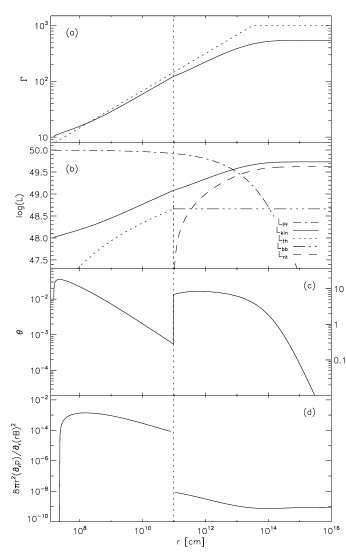
Figure 1: Solution for $L=10^{50}\,\mathrm{erg\,s^{-1}\,sterad^{-1}}$, $\sigma_{0}=100$ (corresponding to an initial Lorentz factor of 10), $\epsilon\Omega=10^{3}\,\mathrm{s^{-1}}$, $\mu=0$. The vertical dotted line indicates the photosphere radius. (a) Lorentz factor where the dotted line represents the analytical approximation derived in Paper II. (b) Various energy fluxes per sterad as labelled in the legend. Indices denote the Poynting flux (pf), kinetic, thermal, black-body (bb) and non-thermal (nt) components. (c) Normalised temperature $\theta=kT/(m_{\mathrm{e}}c^{2})$. The matter is rather cold and pairs do not play a role since $\theta\ll 1$. The temperature jump at the photosphere is no real discontinuity but rather a rapid but steady change. This is the result of the abrupt change in the equation of state from a radiation dominated to a matter dominated fluid. (d) Ratio between the thermal pressure gradient and the magnetic force density in the flow. The acceleration is completely determined by the magnetic field at all radii.

As an example, Fig. 1 shows the result of a numerical integration. The result can be compared with the analytical approximation derived in Paper II. The analytic estimate gives a fair representation of the full results, though it overestimates the terminal Lorentz factor somewhat.

The luminosity carried by the medium $L_{\mathrm{mat}}=w/(\rho c^{2})\Gamma\dot{M}c^{2}$ is made up of the kinetic $L_{\mathrm{kin}}=\Gamma\dot{M}c^{2}$ and the thermal part $L_{\mathrm{th}}=(w/(\rho c^{2})-1)\Gamma\dot{M}c^{2}$. The fact that the fluid is dominated by the pressure and energy density of the radiation in the optically thick region can be seen at the photosphere. Fig. 1c displays that a major part of the thermal energy flux $L_{\mathrm{th}}$ is made up from the radiation component which is released as black body radiation at the photosphere. This explains why the thermal energy flux $L_{\mathrm{th}}$ in Fig. 1b nearly coincides with the black body luminosity $L_{\mathrm{bb}}$.

Outside the photosphere $\Gamma$ (and therefore $L_{\mathrm{kin}}$) becomes smaller than the analytical estimate. The non-thermal radiation flux component $L_{\mathrm{nt}}$ rises quickly and the dissipated energy is efficiently converted into radiation. The fractions of the total luminosity converted to kinetic, thermal, and non-thermal energy in this example are 54%, 5%, and 41%, respectively. This demonstrates the high efficiency of the magnetic dissipation process in accelerating the flow and the production of non-thermal radiation.

In Paper II we neglected the thermal pressure and one could argue that the acceleration obtained in the present study should be somewhat greater due to the additional effects of the finite thermal pressure gradient of the matter and radiation component. To compare the magnetic and thermal contribution to the acceleration we regard the momentum eq. (13) which reads in non-conservative form

$$\frac{1}{r^{2}}\partial_{r}r^{2}wu^{2}+\partial_{r}p=\frac{1}{c}\left(\@vec{j}\times\@vec{B}\right)_{r}=\frac{\partial_{r}(rB)^{2}}{8\pi r^{2}}\ .$$ (39)

The ratio between the thermal pressure gradient $\partial_{r}p$ and the magnetic force density $\left[\partial_{r}(rB)^{2}\right]/\left(8\pi r^{2}\right)$ is plotted in Fig. 1d for our chosen example parameter set. At the photosphere the ratio decreases since the radiation component drops out. But even if radiation is included the total thermal pressure gradient is not important compared to the magnetic force density which determines the dynamics of the flow. Thus the radiation pressure can be neglected above the photosphere without influencing the dynamics of the flow.

3 Shortest time scales

Though the model presented here is stationary and thus does not describe the variability of GRBs, we can check whether the physical model on which it is based is compatible with the observed millisecond variations. If the outflow contains inhomogeneities, say, regions where the reconnection proceeds faster or unsteady the flow will show more ore less bright patches. In this section we show that the emission time of these patches will be short enough for GRBs.

The time it takes for the magnetic field to dissipate sets the limit for the shortest emission duration of a single patch in the flow. The time interval $\mathrm{d}t=\mathrm{d}r/c$ in which a flow element moves outward by $\mathrm{d}r$ is Doppler boosted to the observed time interval $\mathrm{d}t_{\mathrm{obs}}=\left(1-\beta\right)\mathrm{d}t\approx\mathrm{d}r/(2c\Gamma^{2})$. Let us assume that the more inhomogeneous flow can still be described approximately by the stationary solution. Using (38) and integrating the observed time from $r=0\ldots r_{\mathrm{sr}}$ gives

$$t_{\mathrm{obs}}=\frac{\pi}{2\epsilon\Omega}=1.6\cdot 10^{-3}\,\mathrm{s}\cdot\left(\epsilon_{-1}\Omega_{4}\right)^{-1}\ .$$ (40)

If the flow consists of shells with differently strong or fast reconnection/emission it can produce observable variations on time scales of the order of milliseconds.

To see if small patches can contribute a significant variability, we note that their lateral size (perpendicular to the flow) is likely to be of the same order as $\lambda=2\pi c/\Omega$. This is the typical size of the small scale field inhomogeneities and the reconnection centres. Due to the short cooling time the emitted radiation originates from close to the reconnection centres so that $\lambda$ is also the lateral size of the bright patches. The overall expansion in the flow does not change the size of the patches if the expansion speed in the comoving frame is always small compared to the Alfvén speed $\approx c$ which is the typical speed with which the magnetic field can reorganise itself. This is the case for $\lambda<r/\Gamma$ being always true at the radii of interest. Thus these patches will stay of the same size $\lambda=$const. and do not scale with radius. $\lambda$ is quite small compared with the radius of the photosphere. The solid angle from which the observed radiation is emitted is of the order $1/\Gamma^{2}$. Hence there are $n=(r/\lambda\Gamma)^{2}=3\cdot 10^{11}\cdot\Omega_{4}^{2}\Gamma_{2}^{-2}r_{13}^{2}$ reconnection patches contributing at any moment to the observed radiation, and the maximum variability amplitude expected is thus $\sqrt{n}/n\approx 2\cdot 10^{-6}$. The observed time scales are not produced locally in the flow but must be due to a variability of the central engine.

4 Parameter study

The parameters of the model are the initial Poynting flux to kinetic energy flux ratio $\sigma_{0}$, the total luminosity per sterad $L$, the fraction of non-dissipatable magnetic field $\mu$, and the measure for the reconnection rate $\epsilon\Omega$. In this section we explore the dependence of the solutions on these parameters, by plotting values of the physical quantities at the photosphere and their asymptotic values at large distances.

4.1 The photosphere

Figure 2: Some physical quantities at the photosphere of the flow as function of the initial Poynting flux ratio $\sigma_{0}$ for different values of the total luminosity per sterad. The values $\epsilon\Omega=10^{-3}\,\mathrm{s^{-1}}$, $\mu=0$ where used. (a) Temperature in the comoving frame. (b) Lorentz factor at the photosphere. (c) Radius of the photosphere. Straight lines in panel (b)+(c) at $200<\sigma_{0}<1000$ indicate the analytical solutions from (41), (42). Thick dots correspond to $\sigma_{0}=\sigma_{0,\mathrm{br}}$ defined in (43).

Figure 2 shows the temperature, Lorentz factor and radius of the flow at the photosphere as functions of the initial Poynting flux ration $\sigma_{0}$. In all plots of the three quantities one can identify a break at a certain value of $\sigma_{0}$. This break can be understood in terms of the saturation radius $r_{\mathrm{sr}}$ mentioned in Sect. 2.7.5. The reconnection yields only little energy beyond $r_{\mathrm{sr}}$ since the largest part of the free magnetic energy is already used up before. The location of this radius relative to the photosphere determines the basic properties of the results. In order to interpret the numerical results, we recall here some the results of the analytic model derived in Paper II. In this model the radius of the photosphere $r_{\mathrm{ph}}$ and the Lorentz factor at the photosphere are given by

$$r_{\mathrm{ph}} = 1.05\cdot 10^{11}\,\mathrm{cm}$$ (41)

$$\cdot\left[\epsilon_{-1}\Omega_{4}\left(\frac{1-\mu^{2}}{0.5}\right)\right]^{-2/5}L_{50}^{3/5}\sigma_{0,2}^{-3/2}\ ,$$

$$\Gamma_{\mathrm{ph}} \approx u_{\mathrm{ph}}=119\cdot\left[\epsilon_{-1}\Omega_{4}\left(\frac{1-\mu^{2}}{0.5}\right)L_{50}\right]^{1/5}\ .$$ (42)

By equating $r_{\mathrm{ph}}$ and $r_{\mathrm{sr}}$ of (41), (36), we find the value of $\sigma_{0}$ where the break in the parameter dependences occurs:

$$\sigma_{0,\mathrm{br}}=39\cdot\left(\epsilon_{-1}\Omega_{4}L_{50}\right)^{2/15}\left(\frac{1-\mu^{2}}{0.5}\right)^{-8/15}\ .$$ (43)

At this value of the baryon loading, the dissipation of magnetic energy ceases around the photosphere. For $\sigma_{0}<\sigma_{0,\mathrm{br}}$ dissipation occurs mostly inside the photosphere, and the radiation is dominated by a black body component.

We note that the analytic expression (41) for $r_{\mathrm{ph}}$ has been derived under the assumption that most of the dissipation occurs outside the photosphere. It is still accurate enough, however, for the estimate (43) that we use to interpret the numerical results. The asymptotic validity of the analytic value (42) of the terminal Lorentz factor $\Gamma_{\infty}$ for large $\sigma_{0}$ is shown in Fig. 2b.

4.2 Limits on thermal and non-thermal radiation

The model yields the luminosity per sterad for both the black-body radiation from the photosphere and the non-thermal radiation. In this section we investigate how these radiation components behave as function of the model parameters and what observed temperatures are expected for the black-body component.

Figure 3: Terminal Lorentz factor and radiation flux ratios as function of the initial Poynting flux ratio $\sigma_{0}$ for different values of the total luminosity per sterad. The values $\epsilon\Omega=10^{-3}\,\mathrm{s^{-1}}$ and $\mu=0$ where used. (a) Terminal Lorentz factor $\Gamma_{\infty}$. The dotted line correspond to the analytical estimates from Paper II where $\sigma_{0}\gg 1$ and no radiative losses were assumed. (b) Ratio between black-body and total luminosity $L_{\mathrm{bb}}/L$ and ratio between non-thermal and total luminosity $L_{\mathrm{nt}}/L$. At the location of the thick dots, the model parameters are such that the magnetic dissipation ceases to be effective near the photosphere [cf. (43)].

Figure 4: Maximal thermal and non-thermal emission as function of $\epsilon\Omega$ (a measure for the dissipation rate). (a) Ratio of maximal thermal emission to dissipatable luminosity $L_{\mathrm{bb,max}}/[(1-\mu^{2})L]$. The used values for $L_{\mathrm{bb,max}}$ correspond to the thick dots in Fig. 3b. (b) Ratio of maximal non-thermal emission to dissipatable luminosity $L_{\mathrm{nt,max}}/[(1-\mu^{2})L]$ determined at $\sigma_{0}=10^{3}$.

Figure 3b displays the luminosities of the thermal and non-thermal radiation components $L_{\mathrm{bb}}$ and $L_{\mathrm{nt}}$ as fraction of the total luminosity $L$. At very low $\sigma_{0}$-values both components are very small. In that case the energy is released far below the photosphere and is converted into kinetic energy. The same happens in ‘dirty fireball’ models where the central engine injects thermal energy into the matter near the source (Shemi & Piran 1990; Paczyński 1990). This also leads to an almost complete conversion into kinetic energy.

The black-body radiation shows its maximum if the dissipation ceases right at the photosphere so that $r_{\mathrm{ph}}=r_{\mathrm{sr}}$. This corresponds to $\sigma_{0}=\sigma_{0,\mathrm{br}}$ from (43). This analytical estimate for $\sigma_{0,\mathrm{br}}$ might be not coincide exactly with the maximum of the numerically obtained $L_{\mathrm{bb}}/L$-curves in Fig. 3b since some simplifications were used in the derivation of (43). Though, we take $L_{\mathrm{bb,max}}=L_{\mathrm{bb}}(\sigma_{\mathrm{0,br}})$ to be the maximal black-body luminosity to simplify the treatment in the following.

From the graphs in Fig. 3b one might guess that the maximal value of $L_{\mathrm{bb}}/L$ does not depend on $L$. Indeed, it turns out that the maximal fraction of the black-body luminosity to the dissipatable luminosity is almost a constant. In the Poynting flux dominated wind the initial Poynting flux luminosity is almost equal to the total luminosity $L_{\mathrm{pf,0}}\approx L$. The fraction of Poynting flux which cannot dissipate by reconnection was parameterised by $\mu^{2}$ so that dissipatable luminosity is $(1-\mu^{2})L_{\mathrm{pf,0}}\approx(1-\mu^{2})L$. If we plot $L_{\mathrm{bb,max}}/[(1-\mu^{2})L]$ as a function of the two other model parameters $\mu,\epsilon\Omega$ we see that its value is around $0.17\pm 0.03$ as displayed in Figure 4a. Thus, the energy in black-body radiation is always less than 20% of the total releasable magnetic energy.

Figure 3b shows that the fraction of the total luminosity emitted as non-thermal radiation has a maximum value for large $\sigma_{0}$ of about 50%, independent of the luminosity itself. In this limit almost all the dissipation takes place outside the photosphere and $L_{\mathrm{bb}}/L$ is negligible.

Figure 4b shows that $L_{\mathrm{nt,max}}/[(1-\mu^{2})L]$ is always very close to $0.5$. The maximal radiation efficiency occurs in the extreme Poynting flux dominated limit. A fast radiation mechanism converts half of the free magnetic energy into non-thermal radiation.

The dissipatable energy flux $(1-\mu^{2})L$, not the total Poynting flux $L_{\mathrm{pf}}\approx L$ in general, is the energy reservoir from which the radiation and kinetic energy is fed. Nevertheless, one needs to know the total Poynting flux in order to determine the absolute magnetic field strength in the medium to investigate the physical emission process. Since this is not needed here we could restrict our study to the case $\mu=0$ in the largest part of this paper. For any combination of $\mu,L$ one finds $\mu^{\prime}=0$, $L^{\prime}=(1-\mu^{2})L$ which yield an outflow of equal dissipatable Poynting flux and thus equal emission and kinetic energy. Therefore, the setting $\mu=0$ has not introduced an additional limitation in the generality of our investigation.

4.3 Limits on the terminal Lorentz factor

In Paper II we derived the terminal Lorentz factor for a complete conversion of Poynting flux into kinetic energy flux. For a Poynting flux dominated flow this terminal Lorentz factor is $\Gamma_{\infty}=(1-\mu^{2})\sigma_{0}^{3/2}$. Since we found that the radiative losses can be as large as 50% of the total luminosity we can now determine upper and lower limits for the terminal Lorentz factor:

$$\frac{1}{2}\left(1-\mu^{2}\right)\sigma_{0}^{3/2}<\Gamma_{\infty}<\left(1-\mu^{2}\right)\sigma_{0}^{3/2}\ .$$ (44)

4.4 Possible variability

The stationary treatment in our study does not yield any variability by definition. But we can speculate about the outcome of quasi-stationary changes in one or more model parameters. The non-thermal luminosity $L_{\mathrm{nt}}$ depends most strongest on $\sigma_{0}$ at moderate values. This is seen in Fig. 3b where the $L_{\mathrm{nt}}/L$ graphs rise quickly to the maximal values in an values around $20\la\sigma_{0}\la 100$. A variation of $\sigma_{0}$ in this moderately large interval might produce some kind of on-off behaviour of the non-thermal luminosity and the large variability in GRB light curves. Extending the model to include time dependence remains an interesting investigation for the future.

4.5 Observable quantities

The results show that a thermal component in the emission is expected at higher baryon loading values. In a limited range of baryon loading ($10\la\sigma_{0}\la 70$), the model predicts a GRB with a significant thermal component. This property can be used observationally as a test of the model, or as a diagnostic of the GRB outflow.

Our model GRBs can be represented in a diagram of showing the ratio $L_{\mathrm{bb}}/L_{\mathrm{nt}}$ as a function of the black body temperature. This is shown in Fig. 5. The photospheric (black body) temperature $T_{\mathrm{obs}}$ shown is the value as observed in the rest frame of the GRB host. It is related to the temperature in a comoving frame $T_{\mathrm{bb}}$ by $T_{\mathrm{obs}}=\Gamma_{\mathrm{ph}}T_{\mathrm{bb}}$.

Figure 5: Thermal to non-thermal flux ratio $L_{\mathrm{bb}}/L_{\mathrm{nt}}$ and redshift corrected temperature of thermal radiation for various model parameters. Calculations for each panel are done for fixed values of $\mu=0$ and $\epsilon\Omega$ as indicated. Solid lines correspond to parameter sets with equal total luminosity $L$ while dotted lines correspond to equal initial Poynting flux ratio $\sigma_{0}$.

The single panels of Fig. 5 show lines for which 3 of the 4 model parameters are fixed while $L$ or $\sigma_{0}$ is varied. An increase in the initial Poynting flux ratio $\sigma_{0}$ increases the temperature but decreases the black-body component due to a smaller photosphere radius (see Fig. 2c). An increase of the total luminosity $L$ results in a larger photosphere temperature and a larger black-body component though the dependence of $L_{\mathrm{bb}}/L_{\mathrm{nt}}$ and $kT_{\mathrm{obs}}$ on $L$ is much weaker than on $\sigma_{0}$.

From Fig. 5 one finds that only low Poynting flux ratios $\sigma_{0}\la 200$ lead to a significant fraction of thermal radiation $L_{\mathrm{bb}}/L_{\mathrm{nt}}\ga 0.1$. The predicted black body temperatures can range all the way from about 5 to 100 keV. These are the temperatures as observed in the frame of the GRB host, so a redshift has to be known in order to use these predictions diagnostically.

Thermal components have indeed been observed in GRB spectra. Preece (2002) reports on a thermal component in the spectra of GRB 970111 within the first $\approx 10\,\mathrm{s}$ after the trigger. In this time interval the temperature of the black body component was observed to vary between 45 and 75 keV, and the ratio of thermal to non-thermal flux was of the order unity. After this initial phase the non-thermal component started to dominate. In terms of our model, these observations indicate that this GRB started with a moderate baryon loading, which then decreased in the course of the burst. Since a redshift of this burst has not been determined, a more detailed comparison with the model can not be made.

4.6 Connection with X-ray flashes

X-ray flashes are fast X-ray transients which are not detected in the $\gamma$-ray band $40$–$700\,\mathrm{keV}$ of BeppoSAX (Heise et al. 2001; Heise & in ’t Zand 2002). In our model this spectral characteristic can be explained by an outflow of low $\sigma_{0}$ where the thermal radiation dominates over the non-thermal component. The relevant region in Fig. 5 would be at $L_{\mathrm{bb}}/L_{\mathrm{nt}}\ga 1$. The temperatures predicted by the model for this range of black body luminosity is $\la 30\,\mathrm{keV}$, which is quite compatible with the observations.

5 Summary and discussion

A magnetised and rotating central engine of a GRB produces a Poynting flux outflow. Any non-axisymmetry of the magnetic field leads to small scale (wave-like) variations in the electromagnetic field carrying energy outward. We have assumed there that these small scale irregularities are subject to rapid reconnection, governed by the Alfvén speed, as observed in other astrophysical settings and in numerical simulations. Thus, the magnetic field can rearrange itself to a energetically favourable configuration and releases its free energy stored in the small scale field variations.

The release of free magnetic energy proceeds with a rate determined by the length scale of the field variation and the local Alfvén speed of the plasma. The magnetic field acts as energy reservoir carried with the matter which transfers its energy to the matter continously. The decay of the magnetic field at the same time causes an outward gradient of the magnetic pressure. This causes a significant part of the Poynting flux to be converted into kinetic energy. The other part of the free energy is converted into heat. In the optically thick region of the flow a thermal energy gradient promotes adiabatic expansion and the conversion of thermal energy to kinetic energy. Thus, at small radii in the optically thick region, almost all of the dissipated magnetic energy gets converted into kinetic energy.

When the flow becomes optically thin at the photosphere the thermal radiation energy escapes to infinity. This radiation resembles a black body spectrum if the photons are created near the photosphere. But if scattering dominates the spectral shape will differ and might look like e.g. a modified black body or a Wien spectrum (Rybicki & Lightman 1979). A much more detailed treatment is necessary to determine the radius at which the radiation is produced and what spectral shape it has. At this stage we are only interested in the total energetics and the characteristic radiation temperature and we assume that the simplified black body treatment give sufficiently precise estimates.

To compute the radiation spectrum from the optically thin region more detailed physics is needed which is beyond the scope of this paper. We have instead assumed that the reconnection process under optically thin conditions maintains a significant population of energetic electrons, which then radiate synchrotron radiation in much the same way as in the standard internal shock model. An advantage of our model is that the magnetic field needed for the synchrotron radiation is a natural part of the flow model itself (see also Paper I). The central difference of the model presented to standard internal shock models for GRBs is that radiation stems from the local dissipation of magnetic energy and not from shock conversion of kinetic energy. Therefore, one does not need an extremely variable central engine to obtain an acceptable radiation efficiency (Beloborodov 2000; Kobayashi & Sari 2001).

The continuous character of the energy release leads to a slower acceleration of the flow compared to the classical fireball scenario. In a fireball the energy is injected abruptly as thermal energy. This leads to an rapid acceleration where the Lorentz factor is linear to the source distance $\Gamma\propto r$. In our model the release of magnetic energy leads to $\Gamma\propto r^{1/3}$ in the optically thick region.

An important model parameter is the ratio between Poynting flux and kinetic energy flux $\sigma_{0}$ at some initial radius $r_{0}$. This parameter controls the baryon loading parameter in a sense that high values correspond to a low baryon loading. The value of $\sigma_{0}$ decides how much of the Poynting flux energy gets converted into kinetic energy, black-body radiation and non-thermal radiation. The three other parameters of the model are the total luminosity per sterad, the fraction of dissipatable Poynting flux and the reconnection speed. There are three intervals of $\sigma_{0}$ values in which the characteristics of the flow is significantly different. At very low values ($\sigma_{0}\la 10$) most of the energy gets converted into kinetic energy. The magnetic energy gets released in the optically thick part. This case is similar to dirty fireball models in which the central engine injects thermal energy into the matter near the central engine (Shemi & Piran 1990; Paczyński 1990). The matter is already cold when it reaches the photosphere at large radii and there is no more free magnetic energy available to power the non-thermal radiation. The burst energy can only power an afterglow by an external shock.

An intermediate Poynting flux ratio of $\sigma_{0}\approx 100$ causes the release of a considerable amount of energy near the photosphere and the thermal emission is non-negligible. The black-body component becomes maximal if the radius where the dissipation ceases coincides with the photosphere. Then, $\approx 17\%$ of the dissipatable magnetic energy gets converted into black-body radiation while the rest ends up in kinetic energy.

At very high $\sigma_{0}\la 300$ values the radius of the photosphere is small and almost all of the dissipation takes place in the optically thin region. The dissipated energy gets equally distributed among the non-thermal radiation and the kinetic luminosity of the flow. At low baryon loading, and for a purely non-axisymmetric magnetic field, almost exactly 50% of the the Poynting is converted into kinetic energy and 50% into non-thermal radiation. If a substantial part of the magnetic field is axisymmetric, the Poynting flux associated with it does not dissipate, and instead is expected to show up as afterglow emission.

Assuming that regular GRBs have large $\sigma_{0}$ this finding predicts that the energy of the afterglow (fed by the kinetic energy of the flow) is comparable to the energy of the the prompt emission. Beaming effects change this picture if the outflow consists of a sufficiently narrow jet. The energy in the afterglow will be weaker because after the flow has decelerated the radiation is spread over a larger solid angle compared to the highly beamed initial radiation (cf. the light curve break discussion in e.g. Ghisellini 2001). Therfore the prompt emission might be more luminous than the afterglow luminosity if the jets points towards us.

Besides the luminosity of the black-body radiation the model yields the temperature of this radiation. We find that the unredshifted observable temperature is $5\,\mathrm{keV}\la kT_{\mathrm{obs}}\la 100\,\mathrm{keV}$ for our fiducial GRB/X-ray burst parameters. The model produces a rather constant Lorentz factor at the photosphere so that large variations of model parameters result in only a small temperature spread. We cannot make a clear statement about the contribution of the non-thermal component to emission in the quoted energy range because we do not know the radiation mechanism. If the thermal component at its maximum is of the same order or greater than the non-thermal component a feature should be present in the spectrum. In fact, there exist observations of excess emission in the low energy range ($\approx 1$–$5\,\mathrm{keV}$) for some GRBs (Strohmayer et al. 1998; Preece et al. 1996). Recent investigations by Preece (2002) show clearly a strong thermal component in the during the first 10 s of GRB 970111 with temperatures of 45–75 keV. These numbers are in agreement with some of our fiducial GRB model parameter values. Observations of this kind will enable us to determine the model parameters and even there time-dependence during the burst.

For initial ratios between Poynting flux and kinetic energy flux $\sigma_{0}\approx 40$ the black-body radiation component dominates over the non-thermal component. The radiation efficiency is lower than in the $\sigma_{0}\ga 300$ case because only $\la 17\%$ of the total luminosity can be converted into radiation. We speculated in Paper II about the possibility that these low-$\sigma_{0}$ outflows could be identified with X-ray flashes observed by BeppoSAX (Heise et al. 2001; Heise & in ’t Zand 2002). Because no dissipation takes place outside of the photosphere there is no non-thermal emission in the $\gamma$-ray range $>40\,\mathrm{keV}$. The present study showed that the thermal emission has an (unredshifted) observable temperature of $\la 30\,\mathrm{keV}$ which agrees with the observations of X-ray flashes. Heise et al. (2001) speculated that X-ray flashes are bursts with high mass loading. This is also true in our model since high mass loading corresponds to low $\sigma_{0}$ values.

The hypothesis that the thermal radiation from a low-$\sigma_{0}$ outflow produces a X-ray flash may be checked by future observation. The model predicts a lower radiation efficiency of $\la 17\%$ so that most of the dissipated energy in the outflow goes into kinetic form. It will be converted into radiation in the external shock of the afterglow. The afterglow of an X-ray flash should be more luminous than the prompt emission if jet-effects do not interfere too much.

A stationary approximation for the flow is used in this paper. If the central engine operates intermittently internal shocks could occur in the magnetised outflow. One could also imagine that not the total luminosity changes with time but that the other wind parameters like the mass loading and with it $\sigma_{0}$ varies. $\sigma_{0}$ has a strong influence on the non-thermal luminosity $L_{\mathrm{nt}}$ and the black-body luminosity $L_{\mathrm{bb}}$. A time-varying $\sigma_{0}$ around intermediate values leads certainly to large modulations in the non-thermal light curve. The physical model should be extended to include time dependent model parameters to investigate their effect on the light curve.

The minimal observed variability of GRBs is around a millisecond. Any process producing the emission must therfore be fast enough to account for this limit. The stationary model predicts that the reconnection in the comoving frame lasts for approximately 1 millisecond. The effects for Doppler shift and relativistic time dilation almost cancel so that one observes almost the time in the comoving frame. The millisecond variability is therfore compatible with the reconnection model. If the reconnection in the flow is not smoothly distributed but patchy we would expect to see a peak for the emission coming from one of the patches where reconnection takes place. Our model is nevertheless applicable because we only need the overall reconnection rate, the average over small length scales, which is responsible for the global flow dynamics.

References

- Begelman & Li (1994) Begelman, M. C. & Li, Z.-Y. 1994, ApJ, 426, 269
- Beloborodov (2000) Beloborodov, A. M. 2000, ApJ, 539, L25
- Biskamp (1986) Biskamp, D. 1986, Phys. Fluids, 29, 1520
- Coroniti (1990) Coroniti, F. V. 1990, ApJ, 349, 538
- Daigne & Drenkhahn (2002) Daigne, F. & Drenkhahn, G. 2002, A&A, 381, 1066
- Daigne & Mochkovitch (1998) Daigne, F. & Mochkovitch, R. 1998, MNRAS, 296, 275
- Drenkhahn (2002) Drenkhahn, G. 2002, A&A, 387, 714
- Ghisellini (2001) Ghisellini, G. 2001, in 2001: A Relativistic Spacetime Odyssey. Experiments and Theoretical Viewpoints on General Relativity and Quantum Gravity, 25th Johns Hopkins Workshop, Florence
- Granot & Königl (2001) Granot, J. & Königl, A. 2001, ApJ, 560, 145
- Heise & in ’t Zand (2002) Heise, J. & in ’t Zand, J. J. M. 2002, in From X-ray Binaries to Gamma Ray Bursts, Jan van Paradijs Memorial Symposium (June 2001), [astro-ph/0112353]
- Heise et al. (2001) Heise, J., in ’t Zand, J. J. M., Kippen, R. M., & Woods, P. M. 2001, in Gamma-Ray Bursts in the Afterglow Era, Rome Workshop (Oct 2000), [astro-ph/0111246]
- Katz (1997) Katz, J. I. 1997, ApJ, 490, 633
- Kobayashi & Sari (2001) Kobayashi, S. & Sari, R. 2001, ApJ, 551, 934
- Königl & Granot (2002) Königl, A. & Granot, J. 2002, ApJ, 574, [astro-ph/0112087]
- Kumar (1999) Kumar, P. 1999, ApJ, 523, L113
- Lyubarsky & Kirk (2001) Lyubarsky, Y. & Kirk, J. G. 2001, ApJ, 547, 437
- Lyutikov (2001) Lyutikov, M. 2001, Phys. Fluids, 14, 963
- Mestel (1968) Mestel, L. 1968, MNRAS, 138, 359
- Mészáros & Rees (1997) Mészáros, P. & Rees, M. J. 1997, ApJ, 482, L29
- Narayan et al. (1992) Narayan, R., Paczyński, B., & Piran, T. 1992, ApJ, 395, L83
- Paczyński (1990) Paczyński, B. 1990, ApJ, 363, 218
- Panaitescu et al. (1999) Panaitescu, A., Spada, M., & Mészáros, P. 1999, ApJ, 522, L105
- Parker (1979) Parker, E. N. 1979, Cosmical magnetic fields: Their origin and their activity (Oxford: Clarendon Press)
- Petschek (1964) Petschek, E. N. 1964, in Proceedings of an AAS-NASA Symposium on the Physics of Solar Flares, ed. W. N. Hess (Washington, DC: NASA), 425
- Piran (1999) Piran, T. 1999, Phys. Rep., 314, 575
- Preece (2002) Preece, R. D. 2002, private communications
- Preece et al. (1996) Preece, R. D., Briggs, M. S., Pendleton, G. N., et al. 1996, ApJ, 473, 310
- Priest & Forbes (2000) Priest, E. R. & Forbes, T. 2000, Magnetic reconnection: MHD theory and applications (New York: Cambridge University Press)
- Rees & Mészáros (1992) Rees, M. J. & Mészáros, P. 1992, MNRAS, 258, 41P
- Rees & Mészáros (1994) —. 1994, ApJ, 430, L93
- Rybicki & Lightman (1979) Rybicki, G. B. & Lightman, A. P. 1979, Radiative Processes in Astrophysics (Wiley)
- Sari & Piran (1997) Sari, R. & Piran, T. 1997, MNRAS, 287, 110
- Shemi & Piran (1990) Shemi, A. & Piran, T. 1990, ApJ, 365, L55
- Spruit (1999) Spruit, H. C. 1999, A&A, 341, L1
- Spruit et al. (2001) Spruit, H. C., Daigne, F., & Drenkhahn, G. 2001, A&A, 369, 694
- Strohmayer et al. (1998) Strohmayer, T. E., Fenimore, E. E., Murakami, T., & Yoshida, A. 1998, ApJ, 500, 873
- Thompson (1994) Thompson, C. 1994, MNRAS, 270, 480
- Usov (1992) Usov, V. V. 1992, Nature, 357, 472
- Weber & Davis (1967) Weber, E. J. & Davis, Jr., L. 1967, ApJ, 148, 217