Degeneracies and scaling relations in general power-law models for gravitational lenses

Abstract

The time delay in gravitational lenses can be used to derive the Hubble constant in a relatively simple way (Refsdal, 1964). The results of this method are less dependent on astrophysical assumptions than in many other methods. For systems with accurately measured positions and time delays, the most important uncertainty is related to the mass model used. Simple parametric models like isothermal ellipsoidal mass distributions seem to provide consistent results with a reasonably small scatter when applied to several lens systems (Koopmans & Fassnacht, 1999). We discuss a family of models with a separable radial power-law and an arbitrary angular dependence for the potential $\psi=r^{\beta}\,F(\theta)$. Isothermal potentials are a special case of these models with $\beta=1$. An additional external shear is used to take into account perturbations from other galaxies. Using a simple linear formalism for quadruple lenses, we can derive $H_{0}$ as a function of the observables and the shear. If the latter is fixed, the result depends on the assumed power-law exponent according to $H_{0}\propto(2-\beta)/\beta$. The effect of external shear is quantified by introducing a ‘critical shear’ $\gamma_{\mathrm{c}}$ as a measure for the amount of shear that changes the result significantly. The analysis shows, that in the general case $H_{0}$ and $\gamma_{\mathrm{c}}$ do not depend on the position of the lens galaxy. Spherical lens models with images close to the Einstein radius with fitted external shear differ by a factor of $\beta/2$ from shearless models, leading to $H_{0}\propto 2-\beta$ in this case. We discuss these results and compare with numerical models for a number of real lens systems.

1 Introduction

Gravitational lenses offer a unique possibility to determine cosmological distances and hence the Hubble constant (Refsdal, 1964). The method avoids using any form of distance ladder and is almost independent of a deeper understanding of astrophysical processes. This has the advantage that possible statistical and systematic uncertainties can be controlled much better than with other methods. Besides the measurement errors of redshifts, positions and time delays, the most important source of uncertainties in using gravitational lenses to determine $H_{0}$ is the mass model of the lens. Constraints provided by observational data are never sufficient to fix the mass distribution uniquely (Saha & Williams, 1997; Williams & Saha, 2000). Simple parametric models, based on the knowledge about typical galaxies in the local universe or desired mathematical properties, are normally used to overcome this difficulty. This approach, while leading to consistent results, has the disadvantage of hiding the underlying uncertainties and making it difficult to quantify them.

In this paper, we consider a family of mass models with separable radial and angular dependence of the potential. External perturbations are included as an external shear. In this way, the different parts can be studied independently. For the radial dependence, we choose a simple power-law and are especially interested in the influence the radial slope has on the results. Several authors (Wambsganß & Paczyński, 1994; Witt et al., 1995; Wucknitz & Refsdal, 2001) have found approximate scaling relations of $H_{0}\propto 2-\beta$ for spherical models with external shear. The same dependence was found before by Chang & Refsdal (1976) for doubles in spherical models without shear (see also Refsdal & Surdej, 1994). The work of Williams & Saha (2000) showed, that the radial slope also has important effects in non-parametric models. Due to the very general nature of these models, no exact scaling law could be found for them.

We follow an intermediate approach by using an arbitrary function only for the angular part. The models include elliptical mass distributions and potentials as well as other shapes. It has been observed in several lens systems, that the external shear required to fit the data with simple elliptical models is much higher than expected. This might indicate a kind of asymmetry of the galaxy that cannot be accounted for by elliptical models. The general angular part of the potential we use can describe this ‘internal shear’ more accurately than simple parametric approaches.

We extend and generalize the work of Witt et al. (2000) by including the three independent time delays in quadruple systems as constraints for the models. We do not use magnification ratios for several reasons. One is the observational problem of reliably measuring correct flux ratios. Fluxes are influenced by microlensing and extinction. These effects can be very strong in the optical and in some cases they are still significant for radio wavelengths. The other reasons are related to our formalism and will be discussed later.

With this approach, we can derive explicit solutions for the Hubble constant as a function of the observables, the power-law exponent $\beta$, and the external shear. We use the results to find a simple but rigorous scaling law describing the dependence of $H_{0}\Delta t$ on $\beta$ in lenses with quadruple images. This scaling law of $H_{0}\Delta t\propto(2-\beta)/\beta$ is also valid for more special parametric power-law models within the allowed range of $\beta$ and is therefore inherent to these models and not an artefact of the general angular dependence we discuss.

The qualitative effect of this scaling law is easily understood when comparing it with the $2-\beta$ scaling discussed before and with the mass-sheet degeneracy, which leads to $H_{0}\Delta t\propto 1-\kappa$. In all cases, a shallower density profile (larger $\beta$ or $\kappa$) leads to smaller values of $H_{0}\Delta t$. The flat part of the density distribution ($\kappa$ in the mass-sheet degeneracy) amplifies the deflection angles but leaves the time delays unaffected. To fit the given geometry, the total deflection angles have to be constant, therefore the time delays ($H_{0}\,\Delta t$) decrease.

We also discuss the effect of the external shear on the time delays and the measured Hubble constant. If the shear is changed, the internal asymmetries of the mass distribution have to be adjusted to compensate for the changes. The total effect of these two contributions will be described by the new concept of a ‘critical shear’ $\text{\boldmath$\gamma$}_{\mathrm{c}}$. The measured Hubble constant is a linear function of the external shear and becomes zero for $\text{\boldmath$\gamma$}=\text{\boldmath$\gamma$}_{\mathrm{c}}$. We will present a simple interpretation of the critical shear in terms of the image geometry.

The main goal of this work is to investigate the uncertainties in measurements of $H_{0}$ or cosmological parameters from time delays in gravitational lenses. The combination of distances that can be determined not only depends on the redshifts and $H_{0}$ but also on the other cosmological parameters ($\Omega$ and $\lambda$ in standard cosmology) and the smoothness of the mean density distribution (‘lumpiness’ parameter $\alpha$). The results will also help in minimizing possible errors, either by selecting lenses with the least uncertainties or by using constraints of the model parameters which are lensing-independent.

Finally, we apply the formalism to several known lens systems, with and without measured time delays, to compare our analytical results with those from numerical model fitting using parametric models. For 2237+0305, we compare with own numerical models and find a very good agreement even though the time delays are not used as constraints in this case.

Our results can be used directly to determine $H_{0}$ from time delays without explicit modelling but should not be used as a substitute for it. They are rather meant to provide an explanation for the degeneracies and scaling relations that have been found for several families of lens models. Nevertheless, we show that the direct application to real systems is possible.

In the appendix, we discuss possible Einstein rings in our family of models. Interestingly, infinitely small sources can be mapped as elliptical rings for arbitrary values of the external shear. The ellipticity of these rings is directly determined by the shear.

2 The lens model

For the lens equation and deflecting potential $\psi$, we use the following notation:

$$z_{\mathrm{s}} =\text{\boldmath$z$}-\text{\boldmath$\alpha$}(\text{\boldmath$z$})$$ (1)

$$\text{\boldmath$\alpha$}(\text{\boldmath$z$}) =\text{\boldmath$\nabla$}\psi(\text{\boldmath$z$})$$ (2)

$$z =r\,\left(\,\cos\theta\,,\,\sin\theta\,\right)$$ (3)

We use a power-law approach with a general separable angular part for the main lensing galaxy.

$$\psi^{\mathrm{(g)}}(\text{\boldmath$z$})=r^{\beta}\,F(\theta)$$ (4)

This family of models includes both elliptical mass distributions and elliptical potentials with arbitrary radial mass index $\beta$. In the following, we assume all image positions as known. For the chosen model, this implies also the knowledge of the position of the galaxy centre itself, because coordinates are relative to this centre. Later we will see, however, that some of the equations are translation invariant, leaving the results unchanged when shifting the galaxy. The limiting cases of $\beta\to 0$ and $\beta=2$ correspond to a point mass and a density constant in the radial direction, respectively. Between these two, the isothermal models are another special case with $\beta=1$. The normalized surface mass density of the general model is

$$\sigma(\text{\boldmath$z$}) =\frac{1}{2}\text{\boldmath$\nabla$}^{2}\psi$$ (5)

$$=\frac{r^{\beta-2}}{2}\Bigl{(}\beta^{2}\,F(\theta)+F^{\prime\prime}(\theta)\Bigr{)}\quad\text{.}$$ (6)

Here and in the rest of this paper, primes indicate derivatives with respect to $\theta$. A very simple relation holds for the radial derivative of the potential which we will need in the time delay equations later:

$$\text{\boldmath$z$}\cdot\text{\boldmath$\nabla$}\psi^{\mathrm{(g)}}=\beta\,\psi^{\mathrm{(g)}}$$ (7)

To account for nearby field galaxies or the contribution of a cluster, we include an external shear plus an additional constant mass density or convergence $\kappa$ into our models. This $\kappa$ can not be determined from observations as a consequence of the so called mass-sheet degeneracy, first discussed by Falco et al. (1985) and Gorenstein et al. (1988). In the following, we therefore always use a fixed $\kappa$. We parametrize the shear as follows:

$$\psi^{(\gamma)}(\text{\boldmath$z$}) =\frac{1}{2}{\text{\boldmath$z$}}^{\text{t}}{\matGamma}\text{\boldmath$z$}$$ (8)

The shear matrix includes both the convergence and the shear itself.

$$=\begin{pmatrix}\kappa-\gamma_{x}&-\gamma_{y}\\ -\gamma_{y}&\kappa+\gamma_{x}\end{pmatrix}$$ (9)

$$\gamma =\gamma\,\left(\,\cos 2\theta_{\gamma}\,,\,\sin 2\theta_{\gamma}\,\right)$$ (10)

With this definition, $\theta_{\gamma}$ points in the direction of the external perturbing mass or equivalently in the opposite direction. Note that this part of the potential is a special case of the power-law with $\beta=2$.

3 Time delays

The light travel time $t$ for a certain image at $z$ can be calculated for arbitrary lens models by using the equation

$$t=\frac{1}{c}D_{\mathrm{eff}}\left(\frac{1}{2}|\text{\boldmath$\alpha$}(\text{\boldmath$z$})|^{2}-\psi(\text{\boldmath$z$})\right)+\text{const}\quad\text{with}$$ (11)

$$D_{\mathrm{eff}}=\frac{D_{\mathrm{d}}\,D_{\mathrm{s}}}{D_{\mathrm{ds}}}\,(1+z_{\mathrm{d}})\quad\text{.}$$ (12)

Here $D_{\mathrm{d}}$ and $D_{\mathrm{s}}$ are angular size distances of the deflector and the source from the observer, while $D_{\mathrm{ds}}$ is the distance of the source measured from the deflector. We separate this equation as usual into one part depending only on cosmology (without $H_{0}$), the contribution from the Hubble constant, and a lens dependent part. This is done by using reduced distances $d_{x}$ (with $D_{x}=d_{x}\,c/H_{0}$) that only depend on the cosmological parameters (and the redshifts) but not on $H_{0}$ itself. We now use a scaled version of the Hubble constant,

$$h=\frac{H_{0}}{d_{\mathrm{eff}}}\quad\text{,}$$ (13)

which includes the cosmological factors and will later be determined by the lensing effect. This $h$ is directly proportional to the Hubble constant itself when the cosmology is fixed. For two images $i$ and $j$, we get a time delay of $\Delta t_{ij}$ with

$$h\,\Delta t_{ij} =h\,(t_{i}-t_{j})$$ (14)

$$=\frac{1}{2}\left(|\text{\boldmath$\alpha$}_{i}|^{2}-|\text{\boldmath$\alpha$}_{j}|^{2}\right)-(\psi_{i}-\psi_{j})\quad\text{.}$$ (15)

By using the lens equation (1), we can transform this expression into a linear functional of the deflecting potential and its derivatives. Mixed terms like $\text{\boldmath$z$}_{i}\cdot\text{\boldmath$\alpha$}_{j}$ for $i\neq j$ can be eliminated, so that the resulting time delay can again be written as the difference of the light travel times $t_{i}$ themselves.

$$h\,t_{i}=-\frac{1}{2}r_{i}^{2}+\text{\boldmath$z$}_{i}\cdot\text{\boldmath$\nabla$}\psi_{i}-\psi_{i}-C$$ (16)

Although it is not immediately noticeable, this equation still is invariant under translations of coordinates. To prove this, one has to apply the lens equation.

For the special potential we discuss here, the relation (7), which also holds for $\psi^{(\gamma)}$ with $\beta=2$, can be used to eliminate the derivatives of the potential and obtain a simple expression only depending on both parts of the potential at the image position:

$$h\,t_{i}=-\frac{1}{2}r_{i}^{2}-(1-\beta)\psi^{\mathrm{(g)}}_{i}+\psi^{(\gamma)}_{i}-C$$ (17)

We retain using the notion of light travel times for each image instead of time delays between the images to keep the equations simple. The $t_{i}$ are defined except for an overall additive constant that gets absorbed into the constant $C$.

The last equation was already presented in Witt et al. (2000) for the special cases of $\beta=1$ including external shear and for the general shearless power-law model.

4 Counting constraints and parameters

Before solving the equations, we want to discuss how many parameters of the model can at most be determined from observations of lens systems with $n$ images, especially $n=4$. See Table 1 and 2 for a list of parameters and constraining equations. As the time delays do not change when adding the same constant to all $t_{i}$, we have to include the constant $C$ as parameter and thus have $n$ constraints with one parameter for this. We might as well have used only the (uniquely defined) $n-1$ time delays without $C$. Both possibilities result in $n-1$ more constraints than parameters just for the time delays.

Table 1: Parameters for the chosen family of models for a system with $n$ images. The $F^{\prime}_{i}$ are needed in the lens equations.

parameters		number
$h$	scaled Hubble constant	1
$\gamma$	external shear	2
$\beta$	power-law exponent	1
$F_{i}$	angular part $F(\theta_{i})$	$n$
$F^{\prime}_{i}$	${\mathrm{d}}F/{\mathrm{d}}\theta$ at $\theta_{i}$	$n$
$\text{\boldmath$z$}_{\mathrm{s}}$	source position	2
$C$	constant in light travel times	1
total	without fluxes	$2n+7$

Table 2: Constraints from observations of image positions and time delays for a system with $n$ images.

constraints		number
$\text{\boldmath$z$}_{i}$	image positions	$2n$
$t_{i}$	light travel times	$n$
total	without fluxes	$3n$

Even for systems with 4 images of one source, it will be impossible to determine all parameters. We therefore decide to fix $\beta$ in the following calculations so that the results can be used to study the dependence of $h$ on the radial mass slope. We will see that, with fixed $\beta$, all equations stay linear.

Another critical parameter is the external shear, which seems to be higher than expected in many detailed lens models. Fixing $\gamma$ for the moment, we will be able to investigate the influence of any uncertainties in the external shear. In the special case of $\beta=1$, it will even be possible to determine $\gamma$ from the constraints, because a number of other parameters do not contribute then.

We do not include fluxes or magnifications, because they would provide only $n-1$ constraints (the independent flux ratios) and at the same time add $n$ more parameters (the second derivatives of the angular part of the potential at the image positions $F^{\prime\prime}_{i}$). The effect, that models get less constrained, when more observations are included in the analysis, is of course unknown in normal parametric models, where the number of parameters is fixed. Our models have an infinite number of parameters, of which only a finite subset is needed to compare with observations. The number of relevant parameters can change when we include more constraints.

Another reason (besides the difficulties in determining fluxes already discussed) is that, in contrast to deflection angles and time delays, magnification ratios are non-linear functionals of the lensing potential, complicating the equations considerably.

5 Lens equations

To exploit the information given by the image positions, we have to insert the power-law potential with shear into the lens equation (1). The derivative of the galaxy part of the potential can be obtained most simply by rotating its polar form to Cartesian coordinates using the transformation matrix

$$\begin{pmatrix}\partial_{x}\\ \partial_{y}\end{pmatrix}=\begin{pmatrix}\cos\theta&-\sin\theta/r\\ \sin\theta&\cos\theta/r\end{pmatrix}\begin{pmatrix}\partial_{r}\\ \partial_{\theta}\end{pmatrix}\quad\text{.}$$ (18)

Written in a form to take into account the role of $\gamma$, $F_{i}$ and $F^{\prime}_{i}$ as unknowns of the equations, this leads to the following equation.

$$\text{\boldmath$z_{\mathrm{s}}$}=(1-\kappa)\,\text{\boldmath$z$}_{i}-r_{i}^{\beta-2}\begin{pmatrix}x_{i}&-y_{i}\\ y_{i}&x_{i}\end{pmatrix}\begin{pmatrix}\beta F_{i}\\ F^{\prime}_{i}\end{pmatrix}+\begin{pmatrix}x_{i}&y_{i}\\ -y_{i}&x_{i}\end{pmatrix}\begin{pmatrix}\gamma_{x}\\ \gamma_{y}\end{pmatrix}$$ (19)

It is easily seen, that this set of $2n$ equations can be used to determine $F_{i}$ and $F^{\prime}_{i}$, assuming $\gamma$ as known:

$$\beta F_{i} =r_{i}^{-\beta}\Bigl{(}(1-\kappa)\,r_{i}^{2}-x_{i}x_{\mathrm{s}}-y_{i}y_{\mathrm{s}}+\gamma_{x}\,(x_{i}^{2}-y_{i}^{2})+2\,\gamma_{y}\,x_{i}y_{i}\Bigr{)}$$ (20)

$$F^{\prime}_{i} =r_{i}^{-\beta}\Bigl{(}y_{i}x_{\mathrm{s}}-x_{i}y_{\mathrm{s}}-2\,\gamma_{x}\,x_{i}y_{i}+\gamma_{y}\,(x_{i}^{2}-y_{i}^{2})\Bigr{)}$$ (21)

6 The general set of linear equations

We now use (20) to express the galaxy potential in the time delay equations (17). We decide to use the light travel times themselves rather than the $H_{0}$-independent time delay ratios as constraints. In this way we can keep the equations linear and the analysis much simpler. As a result, the following set of equations is obtained for $i=1\dots n$:

$$\begin{split}(1-\kappa)\,r_{i}^{2}\;&+\;(x_{i}^{2}-y_{i}^{2})\,\gamma_{x}\;+\;2x_{i}y_{i}\,\gamma_{y}\\ \;&+\;\frac{2\beta}{2-\beta}\,(t_{i}\,h+C)\;=\;2\frac{1-\beta}{2-\beta}\,\text{\boldmath$z$}_{i}\cdot\text{\boldmath$z_{\mathrm{s}}$}\end{split}$$ (22)

The most interesting fact, besides the linearity, is the simple way the mass index $\beta$ appears in the equations. By combining information from the time delay and lens equations the way we did, it was possible to remove the terms with $\beta$-dependent exponents. Now $\beta$ only contributes in the scaling factors of the unknown parameters. Having solved the system for one value of $\beta$, we immediately find the general solution by scaling $h$, $z_{\mathrm{s}}$ and $C$ with the appropriate factors.

7 The isothermal model

In the case $\beta=1$, the equations (22) obviously degenerate with respect to the source position $z_{\mathrm{s}}$. It is then impossible to constrain the latter, but the same information can now be used to determine the external shear. In this case, the inclusion of the lens equations to determine the parameters $F_{i}$ of the galaxy potential was not really necessary, because $\psi^{\mathrm{(g)}}$ does not contribute to the time delay equations (17). We can now directly invert the latter or (22) to obtain solutions for $h_{\mathrm{iso}}$ and $\text{\boldmath$\gamma$}_{\mathrm{iso}}$.

The transition from exactly isothermal to nearly isothermal models deserves some attention. Even for models with $\beta$ differing only slightly from unity, $\gamma$ is a free parameter, while it is fixed by the observational data for $\beta=1$. An incorrect external shear for almost isothermal models is usually compensated for by diverging source positions and $F_{i}$ and $F^{\prime}_{i}$, leading to unrealistic models. It therefore seems appropriate to use the correct isothermal shear even for models that do not exactly obey $\beta=1$. However, one has to take into account possible measurement uncertainties that introduce errors into $\text{\boldmath$\gamma$}_{\mathrm{iso}}$. Especially the time delays, which all contribute to the solution, can introduce significant uncertainties.

8 Solution for the general model

In the general case with $\beta\neq 1$, (22) can be solved directly to determine $h$ for a given shear $\gamma$. Even without writing the explicit solution, we see, that

$$h\propto\frac{2-\beta}{\beta}(1+g_{x}\,\gamma_{x}+g_{y}\,\gamma_{y})$$ (23)

for some constants $g_{x}$ and $g_{y}$. The Hubble constant scales with $(2-\beta)/\beta$ and is a linear (but not proportional) function of the shear. Notably, the isothermal model plays no special role in this equation, despite the fact that, strictly speaking, $\gamma$ can not be chosen freely in this case. As the isothermal shear is usually only weakly constrained due to the limited measurement accuracy, we may, however, use different values of $\gamma$ even for $\beta=1$. This is always true when the constraints we used here are not all available. Considering this, one might well apply equation (23) regardless of the value of $\beta$.

9 The ‘Critical shear’

As the Hubble constant is linear in $\gamma$, there has to be a one-dimensional family of values of the shear with vanishing $h$. The shear with the smallest absolute value from this family will now be called the ‘critical shear’ $\text{\boldmath$\gamma$}_{\mathrm{c}}$. If we denote the shearless value with $h_{0}$, we can write the effect of external shear as

$$\frac{h}{h_{0}}=1-\frac{\text{\boldmath$\gamma$}\cdot\text{\boldmath$\gamma$}_{\mathrm{c}}}{\gamma_{\mathrm{c}}^{2}}\quad\text{.}$$ (24)

If $\gamma$ and $\text{\boldmath$\gamma$}_{\mathrm{c}}$ point in the same direction, this scaling factor can be written as $1-\gamma/\gamma_{\mathrm{c}}$ which is analogous to the scaling of $1-\sigma/\sigma_{\mathrm{c}}$ for an additional mass sheet $\sigma$ with critical density $\sigma_{\mathrm{c}}$. The critical shear does not dependent on $\beta$ or the time delays $t_{i}$ and can be calculated from the image positions alone.

If an upper bound of $\gamma_{\mathrm{max}}$ can be assumed, this translates to a range of

$$h_{\mathrm{\bigl{(}\begin{smallmatrix}\mathrm{max}\\ \mathrm{min}\end{smallmatrix}\bigr{)}}}=\left(1\pm\frac{\gamma_{\mathrm{max}}}{\gamma_{\mathrm{c}}}\right)h_{0}\quad\text{.}$$ (25)

The critical shear is thus a measure for the amount of external shear that can change $h$ significantly. The larger it is, the smaller the influence of uncertainties in the shear on the determined Hubble constant. Shear in the direction of $\text{\boldmath$\gamma$}_{\mathrm{c}}$ contributes maximally, in a perpendicular direction the influence vanishes. With the ‘direction of shear’, we mean in this context the orientation $2\theta_{\gamma}$ of the vector $\gamma$. This is not the direction of $\theta_{\gamma}$ towards the perturbing mass, cf. eq. (10). External field galaxies located perpendicular to the direction of maximal effect change $h$ by the same amount but with opposite sign. There are, however, four directions where external masses do not contribute. See section 13 for actual numbers of the critical shear in real observed lens systems.

Geometrical interpretation

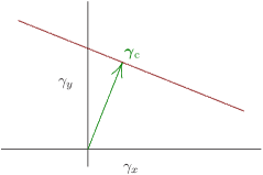
Figure 1: Example critical shear $\text{\boldmath$\gamma$}_{\mathrm{c}}$ (arrow) and values of $\gamma$ for which $h/h_{0}=0$ (straight line). Note that the direction of $\gamma$ is $2\theta_{\gamma}$ and not the direction to the perturbing mass $\theta_{\gamma}$.

For constant light travel times or $h=0$, equation (22) describes an ellipse whose axes $a$ and $b$ are related to the external shear by

$$\frac{\gamma}{1-\kappa}=\frac{a^{2}-b^{2}}{a^{2}+b^{2}}\quad\text{.}$$ (26)

For $\gamma>1-\kappa$, this becomes a hyperbola. The position angle of the minor axis is the same as that of the perturbing mass responsible for the shear ($\theta_{\gamma}$). This means, that each ellipse/hyperbola passing through all images corresponds to a value of $\gamma$ with $h/h_{0}=0$. According to equation (24), for these values

$$\text{\boldmath$\gamma$}\cdot\text{\boldmath$\gamma$}_{\mathrm{c}}=\gamma_{\mathrm{c}}^{2}$$ (27)

holds. The values of $\gamma$ for all these conic sections span the complete subspace for which $h/h_{0}=0$ (see Fig. 1). The critical shear is the smallest of these values and can therefore be calculated with equation (26) for the ‘roundest’ ellipse passing through all images. In Figure 2, we show several such ellipses for some lens systems.

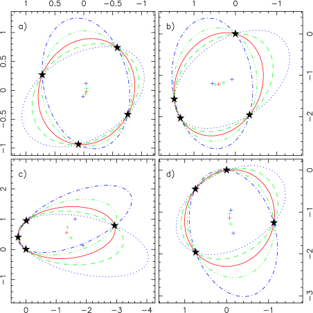
Figure 2: Ellipses passing through all images (stars) of four lens systems. The ‘roundest’ one, which corresponds to the critical shear, is shown as solid line. The centres are shown as crosses. For each ellipse, a shear for which $h/h_{0}=0$ can be calculated by using equation (26). a) Q2237+0305, b) PG 1115+080, c) RX J0911.4+0551, d) B1608+656

We conclude, that for certain values of $\gamma$ (see Figure 1), e.g. for $\text{\boldmath$\gamma$}=\text{\boldmath$\gamma$}_{\mathrm{c}}$, all time delays vanish. Each of the fitting ellipses can act as an Einstein ring for the correct value of $\gamma$. The light travel time is the same for all parts of such rings as Fermat’s theorem requires. In our consideration, the potential is only constrained at the image positions and arbitrary in other directions. The Einstein ring may therefore break up and form a number of discrete images with still vanishing time delays (see appendix).

10 Shifting the lensing galaxy

Surprisingly, most of the quantities we determined do not depend on the position of the lens centre. A shift of the centre is equivalent to adding a constant displacement to the vectors $\text{\boldmath$z$}_{i}$ and $z_{\mathrm{s}}$. If we look at the general set of equations (22), we see that such a shift adds terms linear in $\text{\boldmath$z$}_{i}$ and a constant to the equations. The constant term can be absorbed in $C$ and (for $\beta\neq 1$) the linear terms in $z_{\mathrm{s}}$. As $C$ and $z_{\mathrm{s}}$ are of no interest, the equations do not change when applying this shift.

This means, that $h$ and the critical shear are translation invariant and can be determined even if the lens position is not known. This is only true for the family of models we analyse here. Simple parametric models usually only fit the data for a specific position of the lens centre.

11 Spherical models for nearly Einstein ring systems

For spherical models, the equations are overdetermined. There are nevertheless systems, which can be fit accurately with this kind of model. It can be shown, that $h_{\mathrm{sph}}/h_{0}$ becomes zero for $\beta\to 0$ to cancel the vanishing denominator in (23) and ensure a finite $h_{\mathrm{sph}}$. It can also be shown, that $\gamma$ is parallel to $\text{\boldmath$\gamma$}_{\mathrm{c}}$ for arbitrary $\beta$. Taken together, this means that for point mass models, we always have $\text{\boldmath$\gamma$}=\text{\boldmath$\gamma$}_{\mathrm{c}}$. The geometrical interpretation can be used to determine the direction of external shear for spherical models without calculations. It is given by the orientation of the minor axis of the roundest ellipse passing through all images. For the systems discussed below (and for point mass lenses), even the absolute value of $\gamma$ can be determined from this ellipse.

For systems, where the $n$ images are all located very close to the Einstein ring at $r_{0}$, we can recover another scaling relation. In this case, the power-law can be interpreted as a local approximation to any radial mass profile, like softened power-law spheres or other models. We assume, that one fitting reference model is known. It is then possible to find a family of other models which are also consistent with the observations.

This was done numerically by Wambsganß & Paczyński (1994) and led to a scaling of $h_{\mathrm{sph}}\propto 2-\beta$. Wucknitz & Refsdal (2001) presented a simple interpretation of this fact in terms of the well known mass-sheet degeneracy (Gorenstein et al., 1988). If we multiply the lens equation $\text{\boldmath$z_{\mathrm{s}}$}=\text{\boldmath$z$}-\text{\boldmath$\alpha$}$ with $1-\kappa$, we get another lens equation with the source position and lensing potential (or deflection angle) scaled with the same factor, plus an additional constant convergence $\kappa$. This means, that lens models given by the deflection angles $\alpha$ and $\tilde{\text{\boldmath$\alpha$}}=(1-\kappa)\,\text{\boldmath$\alpha$}+\kappa\,\text{\boldmath$z$}$ are equivalent, but source positions, time delays, etc. are scaled by $1-\kappa$ in the latter model.

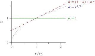
Figure 3: The deflection angles for the three equivalent lens models. The isothermal ($\beta=1$) reference model is shown solid, the transformed model dashed and the final equivalent power-law model dotted.

As reference model, we choose an exponent $\beta_{0}=1$. This model is now transformed as just described and then approximated locally near $r_{0}$ by a modified power law with exponent $\beta$. Figure 3 illustrates this idea. For the new exponent, we find

$$2-\beta=1-\kappa\quad\text{.}$$ (28)

As time delays, source position and external shear all scale with $1-\kappa$, we find the general scaling laws

$$\text{\boldmath$z_{\mathrm{s}}$}\propto 2-\beta,\quad h_{\mathrm{sph}}\propto 2-\beta,\quad\text{\boldmath$\gamma$}\propto 2-\beta$$ (29)

for an arbitrary mass index $\beta$. The time delay ratios do not change.

With $\text{\boldmath$\gamma$}=\text{\boldmath$\gamma$}_{\mathrm{c}}$ for point mass systems, the shear for arbitrary $\beta$ becomes $\text{\boldmath$\gamma$}=\text{\boldmath$\gamma$}_{\mathrm{c}}\,(2-\beta)/2$, leading to a ratio of the Hubble constants for the spherical and shearless case of

$$\frac{h_{\mathrm{sph}}}{h_{0}}=\frac{\beta}{2}\quad\text{.}$$ (30)

The two models differ significantly for a realistic range of $\beta$.

12 Influence of the radial mass index $\mn@boldsymbol{\beta}$

One of the interesting properties of equation (23) is the very simple dependence of the results on $\beta$. The determined value of the Hubble constant $h$ simply scales with the factor $(2-\beta)/\beta$. The most alarming fact is, that this factor does not depend on the geometry of the lens, the time delay ratios or the amount of external shear. When using the models described here to determine $H_{0}$ from lens time delays, the error due to the assumption of an incorrect $\beta$ will be exactly the same for all lens systems as long as the real $\beta$ is more or less equal for all lensing galaxies.

Witt et al. (2000) numerically found a scaling of $(2-\beta)/\beta$ in the case of a power-law model without external shear for orthogonal image pairs ($\theta_{i}-\theta_{j}\approx 90^{\circ}$), while these computations lead to $2-\beta$ for opposed images. In contrast to their work, we have used all time delays as constraints so that they cannot scale differently. The common scale factor of all time delays shows as a scaling of $h$ in our calculations.

The reader might feel as uneasy about the seemingly diverging time delays or $h$ in the limit $\beta\to 0$ as the author did. This limit is equivalent to point mass models and one should not observe diverging time delays for this kind of lens. The point causing trouble here is the fixed external shear in our considerations. To fit the data with a point mass model, the shear has to be equal to the critical shear $\text{\boldmath$\gamma$}_{\mathrm{c}}$. Taking this into account, the result gets multiplied by a vanishing $h/h_{0}\propto\beta$ which cancels the $1/\beta$ factor. If we now change the shear by a small amount, the potential and thus $h$ will immediately diverge in the limit of small $\beta$. This has no direct physical implications, because the mass models will become extremely unphysical to compensate for the shear effect. Small relative differences in the $F_{i}$, that will be introduced by an incorrect shear, will lead to enormous asymmetries in the mass distribution. This is related to the fact, that realistic compact mass distributions can provide only almost spherically symmetric potentials. Any multipole moments would radially decrease more rapidly than the monopole term and must be very strong to have any effect. We will discuss this in more detail for a special case in section 13.1.

For spherical systems with images near the Einstein ring, we confirmed the approximate scaling of $h_{\mathrm{sph}}\propto 2-\beta$. This seems to be incompatible with the general scaling law of $h_{0}\propto(2-\beta)/\beta$ at first sight. With the factor of $h_{\mathrm{sph}}/h_{0}=\beta/2$ from equation (30), by which the shear changes the result in spherical models, these two results are, however, in perfect agreement.

13 Application to special cases

To illustrate the results, we have presented here, and to test their relevance for real lenses, we want to apply the formalism to systems with a special Einstein cross like symmetry and to some of the known real systems that are either useful to actually determine $H_{0}$ (1115+080, 0911+0551, 1608+656) or are interesting because they are very well studied systems like 2237+0305. The calculations will show, that both scaling relations ($h_{\mathrm{sph}}\propto 2-\beta$ and $h_{0}\propto(2-\beta)/\beta$) are relevant for the determination of $H_{0}$ from time delays. The detailed numerical models for 2237+0305 will furthermore show, that the scaling also applies if the time delays themselves are not used to constrain the models. All time delays scale almost exactly as predicted by our analytical work. We will also see that parametric models may fit only for a limited range of $\beta$. The scaling relations are then valid only within this range.

Besides the effects of the exponent $\beta$, the possible strong effects of any external shear will also be confirmed by the numerical models.

13.1 Symmetric Einstein cross like systems

A rather special example of systems shall be discussed explicitly in this section. We consider a lens with time delays $\Delta t_{12}=\Delta t_{34}=0$ and the following image positions:

$$x_{1,2} =\pm(1-\varepsilon)\,r_{0}\qquad y_{1,2} =0$$ (31)

$$x_{3,4} =0 y_{3,4} =\pm(1+\varepsilon)\,r_{0}$$ (32)

From these data, we immediately conclude $\text{\boldmath$z_{\mathrm{s}}$}=0$. The $y$-component of the shear does not contribute at all and cannot be constrained. The equation determining the Hubble constant now reads

$$h\,\Delta t_{13}=(1-\kappa)\,r_{0}^{2}\,\frac{2-\beta}{\beta}2\,\varepsilon\left(1-\frac{\gamma_{x}}{\gamma_{\mathrm{c}}}\right)\quad\text{,}$$ (33)

with the critical shear

$$\gamma_{\mathrm{c}}=(1-\kappa)\,\frac{2\,\varepsilon}{1+\varepsilon^{2}}\quad\text{.}$$ (34)

The special symmetry makes it possible to choose any value of external shear even for isothermal models. Furthermore, it is possible to exactly reproduce the data with spherically symmetric models plus external shear. In this case, the shear is uniquely defined:

$$\gamma =(1-\kappa)\,(2-\beta)\,\varepsilon+{\cal O}(\varepsilon^{2})$$ (35)

The time delay equation now becomes somewhat more complicated than in the non-spherical case. To first order in $\varepsilon$, it reads

$$h_{\mathrm{sph}}\,\Delta t_{13} =(1-\kappa)\,r_{0}^{2}\,(2-\beta)\,\varepsilon+{\cal O}(\varepsilon^{2})\quad\text{.}$$ (36)

Comparing this with (33), we recover the factor of $\beta/2$ between the spherical and shearless case. Both models fit the data exactly and, in this special case, the models are even compatible with highly popular elliptical mass distributions. That means that without any independent information about the external shear (or equivalently the ellipticity of the galaxy itself), we have a factor of two uncertainty even when only considering these two simplest models for $\beta=1$. The real situation may be even much worse, when we consider models with internal and external shear. In this case, any small unknown contribution of external shear of the order of $\gamma_{c}$ (which for very symmetric systems becomes arbitrarily small) will change the result significantly.

Witt et al. (1995) discussed exactly the same type of systems with spherical models plus shear. With $\gamma$ fixed, they also derived a scaling law of $(2-\beta)/\beta$ (see their equation 8). When the shear is constrained by the lens equations, the scaling changes to the $2-\beta$ form.

We finally want to discuss the consequences of diverging time delays in the fixed shear case for $\beta\to 0$ due to equations (23) and (33). For simplicity, we assume $\text{\boldmath$\gamma$}=0$, $\kappa=0$ and $\varepsilon\ll 1$, but the argument is generally also true for other values. We write the potential as a multipole expansion

$$\beta\,F(\theta)=r_{0}^{2-\beta}\left(1-\sum_{k=1}^{\infty}a_{k}\cos 2k\theta\right)\quad\text{.}$$ (37)

To be compatible with equation (20), the coefficients have to meet the condition

$$\sum_{k=1}^{\infty}a_{k}=(2-\beta)\,\varepsilon\quad\text{.}$$ (38)

We notice, that densities (6) can become negative near the axes. To minimize the angular density contrast, we have to keep only the monopole and quadrupole terms and set all higher coefficients to 0. The potential is then equivalent to a density of

$$\sigma=\frac{\beta}{2}\Bigl{(}\frac{r}{r_{0}}\Bigr{)}^{\beta-2}\biggl{(}1+\varepsilon\,(2-\beta)\,\Bigl{(}\frac{4}{\beta^{2}}-1\Bigr{)}\cos 2\theta\biggr{)}\quad\text{,}$$ (39)

which is everywhere positive only for sufficiently high values of $\beta$. When using realistic mass models, we can therefore expect a lower bound for $\beta$ to achieve acceptable fits. This applies not only to this special symmetric lens system but is true in general. Numerical models presented in the next section will confirm this result for $\gamma=0$ (see Figure 4).

13.2 The Einstein cross Q2237+0305

This lens is not usually taken into consideration when thinking about determination of $H_{0}$, because the time delays are expected to be very small and can therefore not be determined easily. Here we show that even if all three time delays were known exactly, constraints for the Hubble constant would still be very weak.

The degeneracy caused by the unknown mass index $\beta$ was already discussed by Wambsganß & Paczyński (1994) for spherical models plus external shear. The authors found the $2-\beta$ scaling using numerical models. We now want to investigate how strong the assumption of a spherical main galaxy really influences the results.

No time delays are available for 2237+0305 and they may never be determined. We can nevertheless calculate the critical shear defined before and compare it with the a typical value one gets for spherical models. Positions including error bars used for this were taken from Crane et al. (1991) to make results comparable with Wambsganß & Paczyński (1994).

The critical shear as calculated from these positions is $\text{\boldmath$\gamma$}_{\mathrm{c}}=(0.0915\pm 0.044,0.0958\pm 0.045)$ or $|\text{\boldmath$\gamma$}_{\mathrm{c}}|=0.13$ where the errors are $1\sigma$ bounds from Monte Carlo simulations. Numerical modelling results in a shear of $0.0696$ almost exactly parallel to $\text{\boldmath$\gamma$}_{\mathrm{c}}$ for isothermal spherically symmetric potentials. We therefore expect the time delays (or $h$ if we take $\Delta t$ as known) of the spherical model with shear to be a factor $0.4745$ smaller than in the shearless case. For the moderately small shear of $\approx 0.07$, this is a huge effect. This factor is in good agreement with the expected value of $1/2$ for idealized systems.

To compare results in the general case, we performed numerical model fitting with an elliptical potential approach plus external shear.

$$F(\theta) \propto\left(\Bigl{(}\frac{\cos\theta}{1+\varepsilon}\Bigr{)}^{2}+\Bigl{(}\frac{\sin\theta}{1-\varepsilon}\Bigr{)}^{2}\right)^{\frac{\beta}{2}}$$ (40)

Elliptical potentials are known to be unphysical for large ellipticities. Although $\varepsilon$ is small in our case, we may expect unrealistic solutions for small values of $\beta$, because the limit of acceptable ellipticities vanishes for $\beta\to 0$ (cf. last section). In fact the fitted $\varepsilon$ also increases with decreasing $\beta$.

We decided not to use invented time delays (calculated for a reference model) to fit the models. In this way, we can check the validity of our results even for cases where multiple time delays are not used as constraints. Plots of the residuals, ellipticity, shear and time delay between component A and B are shown in Figure 4.

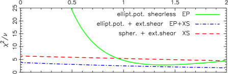
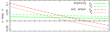
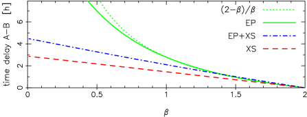
Figure 4: Results of numerical model fitting. The top panel shows the reduced $\chi^{2}$ for the best models. Here $\beta$ was counted as fixed, resulting in $\nu=3\,/\,3\,/\,1$ degrees of freedom for the spherical / shearless elliptical potential / general elliptical potential model, denoted as XS / EP / EP+XS. In the middle, both components of the shear and ellipticity are plotted for the EP+XS model. The last panel presents the time delay A$-$B in hours for $H_{0}=75\,\mathrm{km\,s^{-1}\,Mpc^{-1}}$ and Einstein-de Sitter cosmology. We also included a curve scaling with $(2-\beta)/\beta$ to compare with the EP case.

The non-vanishing residuals at $\beta\to 2$ might be worrying at first, because a spherical model without external shear can fit any image configuration for $\beta=2$. The result would be a sheet of constant density equal to the critical density. There would be no isolated images but an area of constant (and very high) surface brightness. One might thus naively think, that residuals should be very small near $\beta=2$. This is not the case. It is true, that the deviations of the projected images will become arbitrary small in the source plane. On the other hand, however, the magnifications diverge in the limit, causing the deviations in the lens plane to stay finite.

Three families of models have to be discussed. First, we fixed the ellipticities at 0 to compare with the results from Wambsganß & Paczyński (1994). The residuals are almost constant for spherical models. The shear and the time delays scale very accurately with $2-\beta$ as in the idealized considerations.

More interesting in our context is the behaviour in the shearless case where we expect to find a $(2-\beta)/\beta$ scaling of the time delays. The $\chi^{2}$ gets unacceptably large for $\beta\ll 1$. In the other cases ($\beta\ga 0.6$), the agreement with the theoretical predictions also shown in Fig. 4 is very good. For isothermal models, the ratio of time delays calculated for the two models (spherical$/$shearless) is 10–20 per cent larger than predicted by the critical shear. This is still a very good agreement considering that the time delays were not used as constraints for the numerical models.

Real lensing galaxies usually are elliptical and also embedded in an external shear field. We therefore also let both $\varepsilon$ and $\gamma$ vary freely in order to minimize $\chi^{2}$. Counting the formal number of constraints and parameters, we expect a minimum of $\chi^{2}=0$. The fact, that $\chi^{2}$ does not vanish is a confirmation of the degeneracy involving shear and ellipticity already discussed by Witt & Mao (1997). The effective number of parameters is therefore smaller then the formal one. Because we notice the ellipticity changing only slightly with $\beta$, a scaling like that in the spherical case is expected. This can indeed be seen in the plot, where the time delay scales with $2-\beta$. Contrary to the spherical case, $\gamma$ does not scale proportional to $2-\beta$ but is additionally shifted by a constant offset. This is due to the fact that part of the shear has been transformed to ellipticity.

We conclude, that both scaling laws for $h$ or the time delays can be relevant, depending on the family of models used. In the case of 2237+0305, however, the influence of external shear is stronger than the effect of $\beta$ for any realistic values of the latter.

13.3 PG 1115+080

Models and their degeneracies for this quadruple system have been studied extensively (e.g. Courbin et al., 1997; Impey et al., 1998; Keeton & Kochanek, 1997; Saha & Williams, 1997; Schechter et al., 1997; Zhao & Pronk, 2001), leading to a variety of more or less realistic mass distributions and a range of values for the Hubble constant between about 40 and $80\,\mathrm{km\,s^{-1}\,Mpc^{-1}}$.

All these authors agree on the importance of taking the effect of a nearby galaxy group into account. Our formalism includes this group as an external shear of the order $\gamma\approx 0.1$. This shear is however not well constrained. Keeton et al. (1997) showed, that the residuals do not change much for ranges of $\gamma\approx 0.06$–$0.2$. With our general family of models, the effect of unknown external shear can be quantified by using the critical shear and equation (24). To calculate $\gamma_{\mathrm{c}}$, we only need image positions relative to an arbitrary reference centre. The uncertainty in the galaxy position, which is usually much higher than in the image positions, does not affect the result. Using the HST observations from Impey et al. (1998) with their claimed accuracy of $0\aas@@fstack{\prime\prime}002$ as a basis for Monte Carlo simulations, we obtain a critical shear of $\text{\boldmath$\gamma$}_{\mathrm{c}}=(0.142\pm 0.002,0.167\pm 0.003)$. Although the ground based positions from Courbin et al. (1997) are not compatible with the HST results within the formal error bars, the critical shear from these data is about the same, $\text{\boldmath$\gamma$}_{\mathrm{c}}=(0.143\pm 0.003,0.160\pm 0.005)$. This means, that any shear of the order 0.1 can change the results for $H_{0}$ significantly. As the uncertainties in $\gamma$ are of this order of magnitude, large effects on $h$ result even for fixed $\beta$.

The formalism we present in this article was not developed to directly determine $H_{0}$ from observations but to study the model degeneracies and scaling laws. One might nevertheless try to use the prescription from section 7 to obtain an estimate for the Hubble constant and the external shear for an isothermal model. The errors of the observational data of course have to be taken into account.

Time delays derived from the same light curves have been published by Schechter et al. (1997) and Barkana (1997). The A component was not resolved in these observations, and time delays were only determined relative to the sum of A₁ and A₂. This is justified by the small time delay between the two, which is expected to be the order of hours. For our Monte Carlo simulations, we assumed a time delay between the A images of $(0\pm 1)$ days.

Results for $H_{0}$ in the isothermal case differ depending on which set of time delays and positions is used. With the redshifts $z_{\mathrm{s}}=1.722$ and $z_{\mathrm{d}}=0.310$ (Tonry, 1998) and an Einstein-de Sitter universe, we obtain values of $H_{0}$ between 47 and $58\,\mathrm{km\,s^{-1}\,Mpc^{-1}}$ with errors between 12 and 30 per cent ($1\sigma$). The external shear is only weakly constrained, but seems to be of the order 0.1. We have to stress, that this result includes all possible isothermal models with arbitrary angular dependence and is thus much more general than elliptical mass distributions. As long as different determinations of the positions and time delays are not consistent with each other within their error bars, any results for $H_{0}$ have to be interpreted with care of course.

13.4 RX J0911.4+0551

This quad, initially discovered as a triple (Bade et al., 1997), has unique geometrical properties and is a strong candidate for time delay determination, although no result has been published yet. Rapid variability has been detected in the X-ray regime, providing the possibility of a determination of all three time delays with unprecedented accuracy (Chartas et al., 2001). Our first models (elliptical potential plus shear, $\chi^{2}\approx 1$) were presented in Burud et al. (1998). The external shear in the best-fitting model is $\gamma=0.32$ and points almost exactly in the direction of a nearby cluster of galaxies.

The redshift and velocity dispersion of this cluster was measured by Kneib et al. (2000) to $z=0.769$ and $\sigma_{v}=(836\begin{smallmatrix}+180\\ -200\end{smallmatrix})\,\mathrm{km\,s^{-1}}$. From this, they derive an absolute shear of $\tilde{\gamma}=0.11\begin{smallmatrix}+0.05\\ -0.04\end{smallmatrix}$ using a SIS model for the cluster.

To compare with lens models, we have to use the reduced shear $\gamma=\tilde{\gamma}/(1-\kappa)$, because the convergence $\kappa$ caused by the cluster was not taken into account explicitly. The mass-sheet degeneracy simply scales all parameters in (22) with $1/(1-\kappa)$. For SIS models, $\tilde{\gamma}=\kappa$ holds and we obtain $\gamma=0.12\begin{smallmatrix}+0.05\\ -0.04\end{smallmatrix}$. This measurement is not in good agreement with the model from Burud et al. (1998). The reduced shear differs by about 0.2, the direction of the two being almost identical. A possible explanation for this discrepancy is the presence of a second galaxy close to the main lens that might change the potential considerably. It is also possible that the internal asymmetry of the main galaxy itself can not be described as an elliptical mass distribution.

To estimate the uncertainty in time delays or the Hubble constant derived from them, we use again the critical shear which is $\text{\boldmath$\gamma$}_{\mathrm{c}}=(-0.553\pm 0.013,0.101\pm 0.005)$ or $|\text{\boldmath$\gamma$}|=0.56$. Even with this very large critical shear, the uncertainty in the real $\gamma$ has significant effects, because it is large as well.

13.5 B1608+656

This system is the first and up to now only quad for which all three independent time delays have been measured (Fassnacht et al., 1999). This offers the unique possibility to apply our method to a system providing the complete set of constraints. HST images show a main lensing galaxy but also a weaker second galaxy between the four images (Jackson et al., 1998). We nevertheless apply the method to B1608+656, if only to see if the effect of a secondary lens can be detected in this way, e.g. by pretending there is a very large external shear. Data for the positions of the images and the main lensing galaxy were taken from Koopmans & Fassnacht (1999). The formal accuracy of the image positions is extremely high, of the order 2–12 $\mu$arcsec. For the Monte Carlo simulations, we used 1 mas scatter in each coordinate to account for possible shifts by local density fluctuations, caused for example by globular clusters (Mao & Schneider, 1998).

We can use the general equation (22) to determine the Hubble constant for shearless models. With the redshifts of $z_{\mathrm{d}}=0.6304$ and $z_{\mathrm{s}}=1.394$ and standard Einstein-de Sitter cosmology, we obtain a value of $H_{0}=(37\pm 5)\,\mathrm{km\,s^{-1}\,Mpc^{-1}}$ for $\beta=1$. The critical shear is $\text{\boldmath$\gamma$}_{\mathrm{c}}=\left(\,0.072\pm 0.001\,,\,0.069\pm 0.001\,\right)$. For isothermal models, equation (22) predicts a shear of about $\text{\boldmath$\gamma$}=\left(\,-0.32\pm 0.02\,,\,-0.11\pm 0.01\,\right)$, depending on which HST image is used to determine the galaxy position. The result for the Hubble constant is $H_{0}=(130\pm 15)\,\mathrm{km\,s^{-1}\,Mpc^{-1}}$.

The enormous differences in both $H_{0}$ predictions is a consequence of the large external shear $\gamma\gg\gamma_{\mathrm{c}}$. No external shear at all is needed to fit the data when including the influence of the second galaxy in the field. The models in Koopmans & Fassnacht (1999) even predict velocity dispersions for both galaxies which are of the same order of magnitude. This is surprising, since the secondary galaxy is much weaker in all bands in the optical images.

14 Discussion

We used a very general semi-parametric lens model approach to study the changes of time delays and the determined Hubble constant with the assumed radial density slope, quantified by the radial mass index $\beta$. By using only linear constraints, it was possible to keep all the fundamental equations linear. This made the study of the $\beta$ dependence easy. For fixed external shear in quadruple lenses, this resulted in the simple scaling law $H_{0}\propto(2-\beta)/\beta$, independent of the lens geometry, the time delay ratios or the external shear. This means, that a systematic error in the assumed $\beta$ will have exactly the same effect on all lenses and will not show as scatter in the results. The good agreement between $H_{0}$ measurements from different lenses (Koopmans & Fassnacht, 1999) should therefore not be taken as evidence for an accurate determination of $H_{0}$. It merely shows, that all lensing galaxies seem to have more or less the same $\beta$.

In nearly isothermal models, a systematic error of only 10 per cent in $\beta$ will result in an error of about 20 per cent in the deduced Hubble constant. To compare the results from lensing not only with each other but also with results derived from other methods, this possible source of error has to be taken into account.

Furthermore, it is important not only to be aware of this effect, but to try and obtain better constraints on the radial mass profile. Possible ways to do this include modelling lenses with multiply imaged extended sources to obtain constraints for the lensing potential at a wide range of distances to the lens centre. Lenses with multiply imaged point sources can constrain the models only at a small number of radii. This should be done not only for systems with measured time delays, but for as many applicable lenses as possible to acquire reliable measurements of $\beta$ for a representative sample of lenses.

Another possibility is the detailed study of the dynamics of lensing galaxies or of other (usually low redshift) galaxies to learn more about the range of realistic galaxy mass profiles and use the results of this analysis to produce more realistic models for the lenses.

We also quantified the effect of external shear by introducing the concept of a ‘critical shear’ $\text{\boldmath$\gamma$}_{\mathrm{c}}$. The effect of $\gamma$ on $H_{0}$ is linear and strongest in the direction of $\text{\boldmath$\gamma$}_{\mathrm{c}}$. For a fixed direction, its amount is proportional to $\gamma/\gamma_{\mathrm{c}}$. The shear has to be exactly critical to fit the observations in point mass lenses. The value of $\text{\boldmath$\gamma$}_{\mathrm{c}}$ can be found in a geometrical way. It is given by the ellipticity of the roundest ellipse passing through all images. For $\text{\boldmath$\gamma$}=\text{\boldmath$\gamma$}_{\mathrm{c}}$ and non-vanishing $\beta$, the time delays $H_{0}\Delta t$ become zero. This is also true for a whole family of models which are represented by the less symmetric ellipses fitting the images. In the appendix, we discuss the relation to possible Einstein rings which are exactly given by these ellipses.

The effect of shear is also the clue in understanding the compatibility of the general scaling law with the simpler one of $h_{\mathrm{sph}}\propto 2-\beta$ for spherical models. In the latter models, the shear is constrained by the observational data and changes $h$ by a factor of $\beta/2$ when compared to shearless models. In cases where spherical models are able to fit the data, the allowed range of $\gamma$ results in an uncertainty of $h$ always covering both models. This may in certain cases only apply for a limited range of $\beta$.

Interestingly, the value of the critical shear and the Hubble constant in the general model (with fixed shear for $H_{0}$) do not depend on the position of the lensing galaxy. This may be of use for systems where this position cannot be determined accurately.

When using more general models or less constraints than in our calculations, the scaling laws still apply. They are only valid for a subset of the possible models then and one would have to expect even larger uncertainties when using the whole set. This also applies for lenses with less than four images. More special models on the other hand, like parametrized elliptical power-law models, may be able to constrain the range of possible results much better. Nevertheless, the scaling laws still apply for the range of models that are compatible with the constraints. Even in these cases, our results may be used to determine $H_{0}$ without explicit modelling.

Appendix A Einstein rings and high image multiplicities

An interesting property of the general power-law models we used in the main part of this paper is the possibility to produce Einstein rings from point sources for arbitrary values of the external shear. For an Einstein ring parametrized by $r=r(\theta)$, all points on this ring must have the same light travel time to meet Fermat’s theorem. For this appendix, we set $\kappa$ and $\gamma_{y}$ to 0 for simplicity. For an arbitrary direction of the shear, we just have to replace $\theta$ by $\theta-\theta_{\gamma}$. We also assume, that $\gamma<1$.

With $t=0$, the general equations (22) describe an ellipse, which is centred on the lens in the special case $\text{\boldmath$z_{\mathrm{s}}$}=0$ or $\beta=1$.

$$r=r_{0}\,(1+\gamma\cos 2\theta)^{-1/2}$$ (41)

The minor and major axes are $r_{0}/\sqrt{1\pm\gamma}$, compatible with equation (26). The potential is in this case an elliptical one

$$F(\theta)=\frac{1}{\beta}\,r_{0}^{2-\beta}\,(1+\gamma\,\cos 2\theta)^{\beta/2}\quad\text{.}$$ (42)

With respect to the tangential caustic, the effects of ellipticity and shear cancel in these models and the caustic degenerates to a point. This is qualitatively different from elliptical mass distributions where the caustic is deformed and overlaps itself, producing areas of higher multiplicities (see below). With arbitrary $z_{\mathrm{s}}$ and $\beta$, the centre of the ellipse is shifted to $\text{\boldmath$z$}_{0}$ with

$$\begin{pmatrix}1+\gamma_{x}&\gamma_{y}\\ \gamma_{y}&1-\gamma_{x}\end{pmatrix}\text{\boldmath$z$}_{0}=\frac{1-\beta}{2-\beta}\text{\boldmath$z_{\mathrm{s}}$}\quad\text{.}$$ (43)

For $\beta\neq 1$, this shift can take any value if $z_{\mathrm{s}}$ is varied. To obtain a globally unique function $F(\theta)$, the centre of the lens has to be located inside of the ellipse.

Even for lens systems with four images, it is always possible to find an ellipse passing through all of them, which can act as an Einstein ring for the corresponding value of $\gamma$ given by the ellipticity. This does not mean, that we always see an Einstein ring for this special value of external shear, as $F(\theta)$ is not constrained for angles between the images.

Small deviations from the Einstein ring case can lead to an arbitrary number of images near the former elliptical ring. Special cases of these systems (singular isothermal ellipsoidal mass distributions with shear) with up to eight images were mentioned by Lopez et al. (1998) and Witt & Mao (2000) and discussed in detail by Keeton et al. (2000). Evans & Witt (2001) present results for shearless models with arbitrary $F(\theta)$. From (20) and (21) we obtain the following condition for an image of a source at $\text{\boldmath$z_{\mathrm{s}}$}=0$:

$$\frac{F^{\prime}}{F}=-\frac{\beta\,\gamma\,\sin 2\theta}{1+\gamma\,\cos 2\theta}$$ (44)

A global solution for this differential equation is given by (42) which leads to the elliptical ring we discussed before. For a number of discrete images, a more general solution is possible:

$$F(\theta)=f(\theta)\,(1+\gamma\,\cos 2\theta)^{\beta/2}$$ (45)

At the positions of the images $\theta_{i}$, (44) has to be met, leading to the simple condition

$$f^{\prime}(\theta_{i})=0\quad\text{.}$$ (46)

As $f(\theta)$ is an arbitrary function, we can easily construct systems with any number of images. The radial coordinates of the images can then be determined to be

$$r(\theta_{i})=\bigl{(}\beta\,f(\theta_{i})\bigr{)}^{1/(2-\beta)}(1+\gamma\,\cos 2\theta_{i})^{-1/2}\quad\text{.}$$ (47)

References

- Bade et al. (1997) Bade N., Siebert J., Lopez S., Voges W., Reimers D., 1997, A&A, 317, L13
- Barkana (1997) Barkana R., 1997, ApJ, 489, 21
- Burud et al. (1998) Burud I., et al., 1998, ApJ, 501, L5
- Chang & Refsdal (1976) Chang K., Refsdal S., 1976, in L’Évolution des Galaxies et ses Implications Cosmologiques, Colloques Int. du CNRS Vol. 263. p. 369
- Chartas et al. (2001) Chartas G., Dai X., Gallagher S. C., Garmire G. P., Bautz M. W., Schechter P. L., Morgan N. D., 2001, ApJ, 558, 119
- Courbin et al. (1997) Courbin F., Magain P., Keeton C. R., Kochanek C. S., Vanderriest C., Jaunsen A. O., Hjorth J., 1997, A&A, 324, L1
- Crane et al. (1991) Crane P., et al., 1991, ApJ, 369, L59
- Evans & Witt (2001) Evans N. W., Witt H. J., 2001, MNRAS, 327, 1260
- Falco et al. (1985) Falco E. E., Gorenstein M. V., Shapiro I. I., 1985, ApJ, 289, L1
- Fassnacht et al. (1999) Fassnacht C. D., Pearson T. J., Readhead A. C. S., Browne I. W. A., Koopmans L. V. E., Myers S. T., Wilkinson P. N., 1999, ApJ, 527, 498
- Gorenstein et al. (1988) Gorenstein M. V., Shapiro I. I., Falco E. E., 1988, ApJ, 327, 693
- Impey et al. (1998) Impey C. D., Falco E. E., Kochanek C. S., Lehár J., McLeod B. A., Rix H. W., Peng C. Y., Keeton C. R., 1998, ApJ, 509, 551
- Jackson et al. (1998) Jackson N., Helbig P., Browne I., Fassnacht C. D., Koopmans L., Marlow D., Wilkinson P. N., 1998, A&A, 334, L33
- Keeton & Kochanek (1997) Keeton C. R., Kochanek C. S., 1997, ApJ, 487, 42
- Keeton et al. (1997) Keeton C. R., Kochanek C. S., Seljak U., 1997, ApJ, 482, 604
- Keeton et al. (2000) Keeton C. R., Mao S., Witt H. J., 2000, ApJ, 537, 697
- Kneib et al. (2000) Kneib J.-P., Cohen J. G., Hjorth J., 2000, ApJ, 544, L35
- Koopmans & Fassnacht (1999) Koopmans L. V. E., Fassnacht C. D., 1999, ApJ, 527, 513
- Lopez et al. (1998) Lopez S., Wucknitz O., Wisotzki L., 1998, A&A, 339, L13
- Mao & Schneider (1998) Mao S., Schneider P., 1998, MNRAS, 295, 587
- Refsdal (1964) Refsdal S., 1964, MNRAS, 128, 307
- Refsdal & Surdej (1994) Refsdal S., Surdej J., 1994, Rep. Prog. Phys., 57, 117
- Saha & Williams (1997) Saha P., Williams L. L. R., 1997, MNRAS, 292, 148
- Schechter et al. (1997) Schechter P. L., et al., 1997, ApJ, 475, L85
- Tonry (1998) Tonry J. L., 1998, AJ, 115, 1
- Wambsganß & Paczyński (1994) Wambsganß J., Paczyński B., 1994, AJ, 108, 1156
- Williams & Saha (2000) Williams L. L. R., Saha P., 2000, AJ, 119, 439
- Witt & Mao (1997) Witt H. J., Mao S., 1997, MNRAS, 291, 211
- Witt & Mao (2000) Witt H. J., Mao S., 2000, MNRAS, 311, 689
- Witt et al. (2000) Witt H. J., Mao S., Keeton C. R., 2000, ApJ, 544, 98
- Witt et al. (1995) Witt H. J., Mao S., Schechter P. L., 1995, ApJ, 443, 18
- Wucknitz & Refsdal (2001) Wucknitz O., Refsdal S., 2001, in Brainerd T. G., Kochanek C. S., eds, Gravitational Lensing: Recent Progress and Future Goals, ASP conf. series, Vol. 237
- Zhao & Pronk (2001) Zhao H., Pronk D., 2001, MNRAS, 320, 401