The AMANDA collaboration

Limits to the muon flux from WIMP annihilation in the center of the Earth with the AMANDA detector

J. Ahrens Institute of Physics, University of Mainz, D-55099 Mainz, Germany E. Andrés Department of Physics, SCFAB, Stockholm University, S-10691 Stockholm, Sweden X. Bai Bartol Research Institute, University of Delaware, Newark, DE 19716, USA G. Barouch Department of Physics, University of Wisconsin-Madison, WI 53706, USA S.W. Barwick Department of Physics and Astronomy, University of California, Irvine, CA 92697, USA R.C. Bay Department of Physics, University of California, Berkeley, CA 94720, USA T. Becka Institute of Physics, University of Mainz, D-55099 Mainz, Germany K.-H. Becker Institute of Physics, University of Mainz, D-55099 Mainz, Germany D. Bertrand Université Libre de Bruxelles, Science Faculty CP230, B-1050 Brussels, Belgium A. Biron DESY-Zeuthen, D-15735 Zeuthen, Germany O. Botner Division of High Energy Physics, Uppsala University. S-75121 Uppsala, Sweden A. Bouchta now at CERN, CH-1211, Genève 23, Switzerland. DESY-Zeuthen, D-15735 Zeuthen, Germany S. Carius Department of Technology, Kalmar University, S-39182 Kalmar, Sweden A. Chen Department of Physics, University of Wisconsin-Madison, WI 53706, USA D. Chirkin Department of Physics, University of California, Berkeley, CA 94720, USA Fachbereich 8 Physik, BUGH Wuppertal, D-42097 Wuppertal, Germany J. Conrad Division of High Energy Physics, Uppsala University. S-75121 Uppsala, Sweden J. Cooley Department of Physics, University of Wisconsin-Madison, WI 53706, USA C.G.S. Costa Université Libre de Bruxelles, Science Faculty CP230, B-1050 Brussels, Belgium D.F. Cowen Department of Physics and Astronomy, University of Pennsylvania, Philadelphia, PA 19104, USA E. Dalberg now at Defense Research Establishment (FOA), S-17290 Stockholm, Sweden. Department of Physics, SCFAB, Stockholm University, S-10691 Stockholm, Sweden C. De Clercq Vrije Universiteit, Dienst ELEM, B-1050 Brussels, Belgium T. DeYoung now at Santa Cruz Institute for Particle Physics, University of California - Santa Cruz, Santa Cruz, CA 95064, USA. Department of Physics, University of Wisconsin-Madison, WI 53706, USA P. Desiati DESY-Zeuthen, D-15735 Zeuthen, Germany J.-P. Dewulf Université Libre de Bruxelles, Science Faculty CP230, B-1050 Brussels, Belgium P. Doksus Department of Physics, University of Wisconsin-Madison, WI 53706, USA J. Edsjö Department of Physics, SCFAB, Stockholm University, S-10691 Stockholm, Sweden P. Ekström Department of Physics, SCFAB, Stockholm University, S-10691 Stockholm, Sweden T. Feser Institute of Physics, University of Mainz, D-55099 Mainz, Germany T.K. Gaisser Bartol Research Institute, University of Delaware, Newark, DE 19716, USA M. Gaug now at IFAE, 08193 Barcelona, Spain. DESY-Zeuthen, D-15735 Zeuthen, Germany L. Gerhardt Department of Physics and Astronomy, University of California, Irvine, CA 92697, USA A. Goldschmidt Lawrence Berkeley National Laboratory, Berkeley, CA 94720, USA A. Goobar Department of Physics, SCFAB, Stockholm University, S-10691 Stockholm, Sweden A. Hallgren Division of High Energy Physics, Uppsala University. S-75121 Uppsala, Sweden F. Halzen Department of Physics, University of Wisconsin-Madison, WI 53706, USA K. Hanson Department of Physics and Astronomy, University of Pennsylvania, Philadelphia, PA 19104, USA R. Hardtke Department of Physics, University of Wisconsin-Madison, WI 53706, USA T. Hauschildt DESY-Zeuthen, D-15735 Zeuthen, Germany M. Hellwig Institute of Physics, University of Mainz, D-55099 Mainz, Germany G.C. Hill Department of Physics, University of Wisconsin-Madison, WI 53706, USA P.O. Hulth Department of Physics, SCFAB, Stockholm University, S-10691 Stockholm, Sweden S. Hundertmark Department of Physics and Astronomy, University of California, Irvine, CA 92697, USA J. Jacobsen Lawrence Berkeley National Laboratory, Berkeley, CA 94720, USA A. Karle Department of Physics, University of Wisconsin-Madison, WI 53706, USA J. Kim Department of Physics and Astronomy, University of California, Irvine, CA 92697, USA B. Koci Department of Physics, University of Wisconsin-Madison, WI 53706, USA L. Köpke Institute of Physics, University of Mainz, D-55099 Mainz, Germany M. Kowalski DESY-Zeuthen, D-15735 Zeuthen, Germany J.I. Lamoureux Lawrence Berkeley National Laboratory, Berkeley, CA 94720, USA H. Leich DESY-Zeuthen, D-15735 Zeuthen, Germany M. Leuthold DESY-Zeuthen, D-15735 Zeuthen, Germany P. Lindahl Department of Technology, Kalmar University, S-39182 Kalmar, Sweden P. Loaiza Division of High Energy Physics, Uppsala University. S-75121 Uppsala, Sweden D.M. Lowder now at MontaVista Software, 1237 E. Arques Ave., Sunnyvale, CA 94085, USA. Department of Physics, University of California, Berkeley, CA 94720, USA J. Ludvig Lawrence Berkeley National Laboratory, Berkeley, CA 94720, USA J. Madsen Department of Physics, University of Wisconsin-Madison, WI 53706, USA P. Marciniewski now at The Svedberg Laboratory, S-75121, Uppsala, Sweden Division of High Energy Physics, Uppsala University. S-75121 Uppsala, Sweden H.S. Matis Lawrence Berkeley National Laboratory, Berkeley, CA 94720, USA C.P. McParland DESY-Zeuthen, D-15735 Zeuthen, Germany T.C. Miller now at Johns Hopkins University, Applied Physics Laboratory, Laurel, MD 20723, USA. Bartol Research Institute, University of Delaware, Newark, DE 19716, USA Y. Minaeva Department of Physics, SCFAB, Stockholm University, S-10691 Stockholm, Sweden P. Miočinović Department of Physics, University of California, Berkeley, CA 94720, USA P.C. Mock now at Optical Networks Research, JDS Uniphase, 100 Willowbrook Rd., Freehold, NJ 07728-2879, USA. Department of Physics and Astronomy, University of California, Irvine, CA 92697, USA R. Morse Department of Physics, University of Wisconsin-Madison, WI 53706, USA T. Neunhöffer Institute of Physics, University of Mainz, D-55099 Mainz, Germany P. Niessen Vrije Universiteit, Dienst ELEM, B-1050 Brussels, Belgium D.R. Nygren Lawrence Berkeley National Laboratory, Berkeley, CA 94720, USA H. Ogelman Department of Physics, University of Wisconsin-Madison, WI 53706, USA Ph. Olbrechts Vrije Universiteit, Dienst ELEM, B-1050 Brussels, Belgium C. Pérez de los Heros cph@tsl.uu.se Division of High Energy Physics, Uppsala University. S-75121 Uppsala, Sweden A. Pohl Department of Technology, Kalmar University, S-39182 Kalmar, Sweden R. Porrata now at L-174, Lawrence Livermore National Laboratory, 7000 East Ave., Livermore, CA 94550, USA. Department of Physics and Astronomy, University of California, Irvine, CA 92697, USA P.B. Price Department of Physics, University of California, Berkeley, CA 94720, USA G.T. Przybylski Lawrence Berkeley National Laboratory, Berkeley, CA 94720, USA K. Rawlins Department of Physics, University of Wisconsin-Madison, WI 53706, USA W. Rhode Fachbereich 8 Physik, BUGH Wuppertal, D-42097 Wuppertal, Germany M. Ribordy DESY-Zeuthen, D-15735 Zeuthen, Germany S. Richter Department of Physics, University of Wisconsin-Madison, WI 53706, USA J. Rodríguez Martino Department of Physics, SCFAB, Stockholm University, S-10691 Stockholm, Sweden P. Romenesko Department of Physics, University of Wisconsin-Madison, WI 53706, USA D. Ross Department of Physics and Astronomy, University of California, Irvine, CA 92697, USA H.-G. Sander Institute of Physics, University of Mainz, D-55099 Mainz, Germany T. Schmidt DESY-Zeuthen, D-15735 Zeuthen, Germany D. Schneider Department of Physics, University of Wisconsin-Madison, WI 53706, USA E. Schneider Department of Physics and Astronomy, University of California, Irvine, CA 92697, USA R. Schwarz Department of Physics, University of Wisconsin-Madison, WI 53706, USA A. Silvestri Fachbereich 8 Physik, BUGH Wuppertal, D-42097 Wuppertal, Germany DESY-Zeuthen, D-15735 Zeuthen, Germany M. Solarz Department of Physics, University of California, Berkeley, CA 94720, USA G.M. Spiczak Department of Physics, University of Wisconsin-River Falls, WI 54022, USA C. Spiering DESY-Zeuthen, D-15735 Zeuthen, Germany D. Steele Department of Physics, University of Wisconsin-Madison, WI 53706, USA P. Steffen DESY-Zeuthen, D-15735 Zeuthen, Germany R.G. Stokstad Lawrence Berkeley National Laboratory, Berkeley, CA 94720, USA O. Streicher DESY-Zeuthen, D-15735 Zeuthen, Germany P. Sudhoff DESY-Zeuthen, D-15735 Zeuthen, Germany K.H. Sulanke DESY-Zeuthen, D-15735 Zeuthen, Germany I. Taboada Department of Physics and Astronomy, University of Pennsylvania, Philadelphia, PA 19104, USA L. Thollander Department of Physics, SCFAB, Stockholm University, S-10691 Stockholm, Sweden T. Thon DESY-Zeuthen, D-15735 Zeuthen, Germany S. Tilav Bartol Research Institute, University of Delaware, Newark, DE 19716, USA M. Vander Donckt Université Libre de Bruxelles, Science Faculty CP230, B-1050 Brussels, Belgium C. Walck Department of Physics, SCFAB, Stockholm University, S-10691 Stockholm, Sweden C. Weinheimer Institute of Physics, University of Mainz, D-55099 Mainz, Germany C.H. Wiebusch now at CERN, CH-1211, Genève 23, Switzerland. DESY-Zeuthen, D-15735 Zeuthen, Germany C. Wiedemann Department of Physics, SCFAB, Stockholm University, S-10691 Stockholm, Sweden R. Wischnewski DESY-Zeuthen, D-15735 Zeuthen, Germany H. Wissing DESY-Zeuthen, D-15735 Zeuthen, Germany K. Woschnagg Department of Physics, University of California, Berkeley, CA 94720, USA W. Wu Department of Physics and Astronomy, University of California, Irvine, CA 92697, USA G. Yodh Department of Physics and Astronomy, University of California, Irvine, CA 92697, USA S. Young Department of Physics and Astronomy, University of California, Irvine, CA 92697, USA

Abstract

A search for nearly vertical up-going muon-neutrinos from neutralino annihilations in the center of the Earth has been performed with the AMANDA-B10 neutrino detector. The data collected in 130.1 days of live-time in 1997, $\sim$ 10⁹ events, have been analyzed for this search. No excess over the expected atmospheric neutrino background has been observed. An upper limit at 90% confidence level has been obtained on the annihilation rate of neutralinos in the center of the Earth, as well as the corresponding muon flux limit, both as a function of the neutralino mass in the range 100 GeV-5000 GeV.

pacs:

95.35.+d, 95.30.Cq, 11.30.Pb

I Introduction

There are strong observational indications for the existence of dark matter in the universe. Measurements of the energy density of the universe, $\Omega_{\mbox{\tiny 0}}$ , from the combined analysis of cosmic microwave background radiation data and high red-shift Type Ia supernovae favor $\Omega_{\mbox{\tiny 0}}\,=\,1$ , with a matter, $\Omega_{\mbox{\tiny M}}$ , and a cosmological constant, $\Omega_{\tiny{\Lambda}}$ , component. Combined with data from rotation curves of galaxies and cluster mass measurements, the matter contribution to $\Omega_{\mbox{\tiny 0}}$ is $0.3\leq\Omega_{\mbox{\tiny M}}\leq 0.4$ . Big Bang nucleosynthesis calculations of primordial helium, lithium and deuterium production, supported by abundance measurements of these elements, set an upper limit on the amount of baryonic matter that can exist in the universe, $\Omega_{\mbox{\tiny B}}\leq 0.05$ (see Ref. Bergstrom:00a, for a recent review of values of $\Omega$ ). Non-baryonic dark matter must therefore constitute a substantial fraction of $\Omega_{\mbox{\tiny M}}$ .

In this paper we present results of a search for non-baryonic dark matter in the form of weakly interacting massive particles (WIMP) using the AMANDA high-energy neutrino detector. The next section contains a brief motivation for WIMPs as dark matter candidates. Section III describes briefly the characteristics of the AMANDA detector in the configuration used for this analysis. Sections IV and V contain a description of the simulation and analysis techniques used. In section VI we discuss the sources of the current systematic uncertainties of our analysis. In section VII we present the results of the analysis and we introduce a novel way of calculating upper limits in the presence of systematic uncertainties. An upper limit on the neutrino-induced muon flux expected from WIMP annihilation in the center of the Earth is derived with this method. A comparison with published muon-flux limits obtained by existing neutrino experiments is presented in section VIII.

II WIMPs as dark matter candidates

Particle physics provides an interesting dark matter candidate as a Weakly Interacting Massive Particle (WIMP). The relic density of particle type $i$ depends on its annihilation cross section, $\sigma$ , as $\Omega_{i}h^{2}\sim 3\times 10^{-27}/\left<\sigma{\mbox{v}}\right>$ (neglecting mass-dependent logarithmic corrections), where $\left<\right>$ indicates thermal average and v is the relative velocity of the particles involved in the collision (see for example Ref. Jungman:96a, ). Weak interactions provide the right annihilation cross section for the WIMPs to decouple in the early universe and give a relic density within the required range to contribute substantially to the energy density of the universe today. This is basically what would be needed to solve the dark matter problem.

In particular, and starting from a completely different rationale, the Minimal Supersymmetric extension to the Standard Model of particle physics (MSSM) provides a promising WIMP candidate in the neutralino, $\chi$ . The neutralino is a linear combination of the B-ino, $\tilde{\mbox{B}}$ , and the W-ino, $\tilde{\mbox{W}}$ , the supersymmetric partners of the electroweak gauge bosons, and of the H ${}^{0}_{1}$ and H ${}^{0}_{2}$ , the neutral Higgs bosons, and it is stable (assuming R-parity conservation, which is further supported to avoid too rapid proton decay). The actual composition of the neutralino can have cosmological consequences since its annihilation cross section depends on it. For example, it has been argued that a mainly W-ino type neutralino would not be cosmologically relevant in the present epoch since it would have annihilated too fast in the early universe to leave any relevant relic density Griest:90a .

Still, the large parameter space of minimal supersymmetry can be exploited to build realistic models which provide relic neutralino densities within the cosmologically interesting region of 0.025 $\lesssim\Omega_{\chi}h^{2}<$ 1. Negative results from searches for supersymmetry at the LEP accelerator at CERN have set a lower limit on the neutralino mass $m_{\chi}>$ 31 GeV (Ref. OPAL:00a, ), while theoretical arguments based on the requirement of unitarity set an upper limit of 340 TeV (Ref. Griest:90a, ). Imposing in addition the condition on $\Omega_{\chi}h^{2}$ mentioned above, only models with m ${}_{\chi}\lesssim$ 10 TeV (Ref. Edsjo:97a, ) become cosmologically interesting.

Neutralinos have a non-negligible probability of scattering off nuclei of ordinary matter. Assuming the dark matter in the Galactic halo is (at least partially) composed of relic neutralinos, elastic interactions of these particles with nuclei in the Earth can lead to energy losses that bring the neutralino below the escape velocity, becoming gravitationally trapped Press:85a ; Freese:86a . For high neutralino masses ( $>$ a few hundred GeV) direct capture from the halo population by the Earth is kinematically suppressed Gould:88a . In this case neutralinos can be accreted from the population already captured by the solar system. Gravitational capture is expected to result in an accumulation of neutralinos around the core of the Earth, where they will annihilate. An equilibrium density is reached when the capture rate equals the annihilation rate. Neutrinos are produced in the decays of the resulting particles, with an energy spectrum extending over a wide range of values and bounded from above by the neutralino mass. Annihilation of neutralinos directly into neutrinos (or light fermion pairs in general) is suppressed by a factor $m_{\small\mbox{f}}^{2}/m_{\chi}^{2}$ due to helicity constraints, where $m_{\small\mbox{f}}$ is the fermion mass.

Neutrino detectors can therefore be used to constrain the parameter space of supersymmetry by setting limits on the flux of neutrinos from the center of the Earth Jungman:96a ; Feng:00a . Note that this indirect neutralino detection will be favored for high neutralino masses, since the cross section of the resulting neutrinos with ordinary matter scales with E_ν.

III The AMANDA-B10 detector

The AMANDA-B10 detector consists of an array of 302 optical modules deployed in ten vertical strings at depths between 1500 m and 2000 m in the South Pole ice cap. The strings are arranged in two concentric circles of 60 m and 120 m diameter respectively. The modules on the four inner strings are separated by 20 m in the vertical direction, while in the outer six strings the vertical separation between modules is 10 m. An optical module consists of a photomultiplier tube housed in a spherical glass pressure vessel. Coaxial cables (in the inner 4 strings) and twisted quad cables (in the outer 6 strings) provide the high voltage to the photomultiplier tubes and transmit the signals to the data acquisition electronics at the surface.

Muons from charged-current high-energy neutrino interactions near the array are detected by the Cherenkov light they produce when traversing the ice. The relative timing of the Cherenkov photons reaching the optical modules allows the reconstruction of the muon track. A more detailed description of the detector is given in Ref. Amanda:00a, . The detector was triggered when a majority requirement was satisfied: an event was recorded if at least 16 modules had a signal within a predefined time window of 2 $\mu$ s. The data taking rate was 100 Hz.

AMANDA-B10 was in operation during the 1997 Antarctic winter. The separation of 300 atmospheric neutrinos from the data sample collected in that period established the detector as a high-energy neutrino telescope Amanda:01a . The array was upgraded with 122 more modules during the antarctic summer 1997/1998 and in 1999/2000 253 additional ones were added, completing the proposed design of 677 optical modules in 19 strings, AMANDA-II Amanda:01b .

IV Signal and Background simulations

IV.1 Simulation of neutralino annihilations

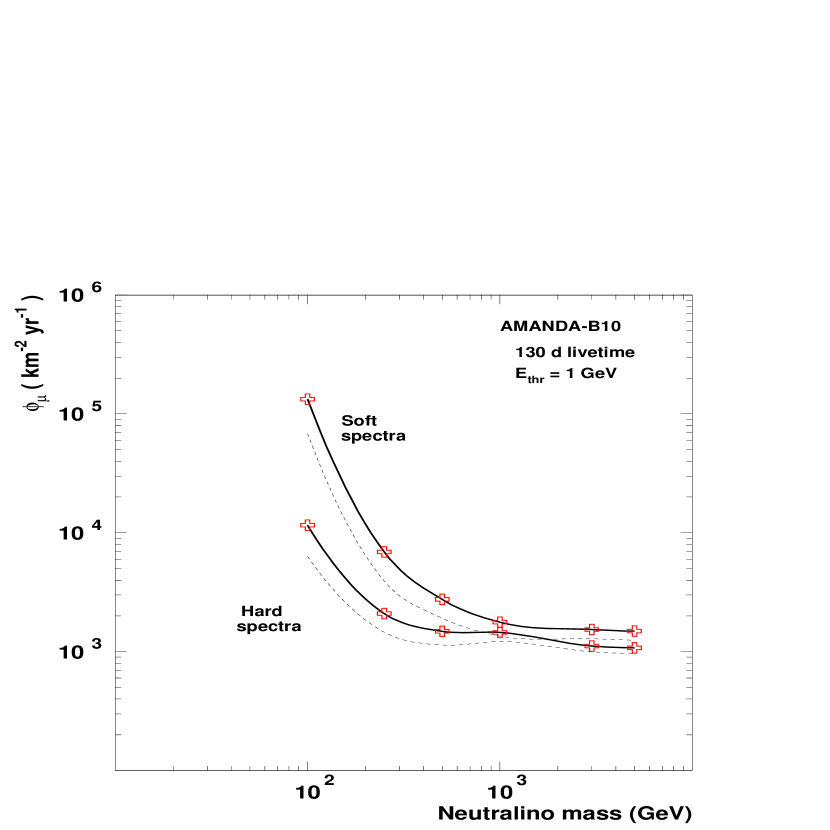
Neutralinos can annihilate pair-wise to, e.g., $\ell^{+}\ell^{-}$ , $\mbox{q}\bar{\mbox{q}}$ , W⁺W^-, Z⁰Z⁰, H ${}^{0}_{1,2}$ H ${}^{0}_{3}$ , Z⁰H ${}^{0}_{1,2}$ and W^±H^∓. Neutrinos are produced in the decays of these annihilation products. Neutrinos produced in quark jets (from e.g. $\mbox{b}\bar{\mbox{b}}$ or Higgs bosons) typically have lower energy than those produced from decays of $\tau$ leptons and gauge bosons. We will refer to the first type of annihilation channels as “soft” and to the second as “hard”.

The simulations of the expected neutralino signal were done in the framework of the SUSY models described in Ref Bergstrom:98a, . The hadronization and decay of the annihilation products have been simulated using PYTHIA PYTHIA . The simulations were performed for six different WIMP masses between 10 GeV and 5000 GeV. For each mass, six different annihilation channels (c $\bar{\mbox{c}}$ , $\mbox{b}\bar{\mbox{b}}$ , $\mbox{t}\bar{\mbox{t}}$ , $\tau^{+}\tau^{-}$ , W⁺W^- and Z⁰Z⁰) were considered, with $1.25\times 10^{6}$ events generated for each. Note that the decay of b– and c–hadrons will take place in matter instead of vacuum. This was incorporated in the simulations in an effective manner justified by the fact that, for the neutralino masses considered, the re-interactions of these heavy hadrons with the surrounding medium are not dominant, and can be parametrized as an effective energy loss at the time of decay. As a reference soft spectrum, we chose the annihilation into b $\bar{\mbox{b}}$ , and as a reference hard spectrum, the annihilation into W⁺W^-. For a given mass, these two spectra can be regarded as extreme cases. We have used these channels in the analysis described below, bearing in mind that a typical spectrum would lie somewhere in between.

IV.2 Simulation of the atmospheric neutrino flux

Neutrinos from the decay of secondaries produced in cosmic ray interactions in the atmosphere constitute the physical background to the neutralino search. We have simulated this atmospheric neutrino flux using the calculations of Lipari Lipari:93a . To obtain the rate of neutrino interactions producing muons we have used the neutrino and anti-neutrino $-$ nucleon cross sections from Gandhi et al. Gandhi:96a . The actual neutrino-nucleon interactions have been simulated with PYTHIA using the CTEQ3 CTEQ3 parametrization of the nucleon structure functions. The use of PYTHIA allows to model the hadronic shower produced at the vertex of the interaction and, therefore, to calculate the Cherenkov light produced by secondaries. When the neutrino-nucleon interaction occurs within the instrumented volume of the detector, this is a non-negligible contribution to the total event light output.

A three-year equivalent atmospheric neutrino sample with energies between 10 GeV and 10 TeV and zenith angles between 90^∘ (horizontal) and 180^∘ (vertically up-going) has been simulated Dalberg:99a . The sample contains 3.7 $\times 10^{7}$ events, of which 41234 triggered the detector.

IV.3 Simulation of the atmospheric muon flux

The majority of the triggers in AMANDA are induced by muons produced in cosmic ray interactions in the atmosphere and reaching the detector depth. The simulation of this atmospheric muon flux was performed using the BASIEV BASIEV program. We note that this program only uses protons as primaries. However, the systematic uncertainty introduced by this approximation is negligible in comparison with that from the present uncertainty in the primary flux intensity. Moreover, heavier nuclear primaries produce more muons per interaction, but with lower energies on average Gaisser:90a , which will in general loose all their energy and decay before reaching the detector. A study performed using the CORSIKA CORSIKA air shower generator, with the QGSJET option to model the hadronic interactions, including the complete cosmic ray composition confirms this scenario.

The simulation of a statistically significant sample of atmospheric muon background is an extremely high CPU-time consuming task due to the strong rejection factors needed. We have simulated 6.3 $\times$ $10^{10}$ primary interactions, distributed isotropically with zenith angles, $\Theta$ , between 0 and 85 degrees, and with energies, E, between 1.3 TeV and 1000 TeV, assuming a differential energy distribution $\propto E^{-2.7}$ (Ref. PDG:00, ). The total number of triggers produced were 5 $\times$ $10^{6}$ . Normalizing to the primary cosmic ray rate, the generated sample corresponds to about 0.6 days of equivalent detector live-time. Due to the narrow vertical angular cones used for this analysis this background sample is sufficient to model the detector response and develop the rejection cuts. In addition, a larger sample of background data was used in the training of the discriminant analysis program used as cut level 4. This is described in more detail in the next section.

Refer to caption — Figure 1: Angular distributions of data and atmospheric muon simulation Monte Carlo (MC) at different analysis levels. Top to bottom: trigger to level 4. The distributions are normalized to the simulated sample, 5 $\times$ 10⁶ events.

IV.4 Muon propagation

The muons produced in the signal and background simulations described above were propagated from the production point to the detector taking into account energy losses by bremsstrahlung, pair production, photo-nuclear interactions and $\delta$ -ray production from Ref. Lohmann:85a, . The Cherenkov light emitted by the secondaries produced in these processes is taken into account when calculating the response of the detector to the passage of the muon.

V Data analysis

The analysis presented in this paper was performed on data taken with the 10-string AMANDA detector between March and November 1997. The experimental data set consists of 1.05 $\times$ 10⁹ events in a total of 130.1 days of detector live-time. The data were first cleaned of noise hits and hits from optical modules that were unstable during the running period. Short pulses, that are likely induced by cross talk between channels are also rejected at this stage. Details on the data cleaning procedure are given in Ref. Amanda:00b, . The data is then reconstructed and five filters consisting of cuts based on the event hit pattern and the quality of the reconstruction are applied in order to identify potential up-going neutrino candidates. The distributions of the reconstructed zenith angle from trigger level (after hit cleaning) until filter level 4 for data and simulated atmospheric muons are shown in figure 1. The curves have been normalized to the simulated sample, 5 $\times$ 10⁶ events. The uppermost curves in the plot show the reconstructed direction without any quality criteria applied to the fits, showing good agreement between the data and the Monte Carlo sample along the whole angular range. The curves clearly indicate that a small percentage (about 2%) of the originally down-going tracks are misreconstructed as up-going (cos $\,\Theta$ less than zero the figure). The series of cuts described below were developed to reject such misreconstructions, and their effect on the angular distribution is also shown in figure 1 for comparison. The filter level 2 and level 3 curves show that the filtering procedure is more effective rejecting the simulated muon background than the data. This is due to detector effects not included in the simulation of the detector response and surviving to these levels, like electronic cross talk between channels or inefficiencies of the digitizing electronics. Other processes not included in the background simulations that can contribute to the discrepancy are overlapping events from uncorrelated cosmic ray interactions and the contribution from electron neutrino induced cascades. To account for this different behavior between data and simulated background under standard cuts, we have used an iterative discriminant analysis as cut level 4 (see subsection V.4) trained on a sub-sample of data (which represents the real remaining background better than the simulations) and a sub-sample of the neutralino signal. A final series of high quality cuts were applied after the discriminant analysis, bringing the remaining data sample to agree with the number of events expected from the known atmospheric neutrino flux, as shown in figure 4 and table 1. Note that the atmospheric neutrino curve and the data curve in figure 4 join and follow each other in the last two steps of the cuts applied within the level 5 filter. The next subsections give a more detailed description of the variables used and the cuts applied at each filter level.

V.1 Filter level 1

In a first stage, a simple and computationally fast filter based on fitting a line to the time pattern of the events, was applied to the data sample in order to reject obvious down-going tracks. This “line fit” (LF) assumes that the known space point of each hit optical module, $\vec{r}_{i}$ , is related to the measured hit time, $t_{i}$ , by $\vec{r}_{i}\,=\,\vec{r}_{o}+\vec{v}t_{i}$ . The minimization of $\chi^{2}\,=\,\sum_{i}(\vec{r}_{i}-\vec{r}_{o}-\vec{v}t_{i})^{2}$ , where the index runs over all the hits in the event, leads to an explicit solution for $\vec{v}$ . The zenith angle of the fitted track is readily obtained as $\cos\Theta_{\mbox{\tiny LF}}=-v_{z}/|v|$ . The angular resolution of the line fit is relatively low since it does not incorporate any information about the geometry of the Cherenkov cone or about scattering of the Cherenkov photons in the ice. Still, its simplicity and computational speed makes it a very useful tool for a first assessment of the track direction and for rejection of down-going atmospheric muons Stenger:90a . The first level filter rejected obvious down-going atmospheric muons by requiring $\Theta_{\mbox{\tiny LF}}>$ 50^∘.

V.2 Filter level 2

The events that pass the level 1 filter are reconstructed using a maximum likelihood approach (ML) as described in Amanda:00a . In short, the ML technique uses an iterative process to maximize the product of the probabilities that the optical modules receive a signal at the measured times, with the track direction (zenith and azimuth angles) as free parameters. The expected time probability distributions include the scattering and absorption characteristics of the ice as well as the distance and relative orientation of the optical module with respect to the track Wiebusch:99a .

The level 2 filter consists of two cuts: the ML-reconstructed zenith angle must be larger than 80^∘ and at least three hits must be “direct”. A hit is defined as direct if the time residual, $t_{\mbox{\tiny res}}$ (the difference between the measured time and the expected time assuming the photon was emitted from the reconstructed track and did not suffer any scattering), is small. Unscattered photons preserve the timing information. Therefore, the reconstruction of the direction of tracks with several direct hits presents a significantly better angular resolution. The number of direct hits associated with a track is the first quality requirement applied to the reconstructed data and simulated samples Amanda:00b . A residual time interval between -10 ns and 25 ns was used to classify a hit as direct at this level.

Figure 2 shows the zenith angle distributions of simulated muon tracks from neutrinos produced in annihilation of neutralinos for the two extreme masses used in this analysis as compared to that from atmospheric neutrinos after filter level 2. The corresponding curve for data and simulated atmospheric muons is included in figure 1. The combined effect of these two filters on the data is a rejection of 98%, as shown in table 1. The efficiencies with respect to trigger level of both level 1 and level 2 filters for simulated neutralino signal are shown in figure 3, for different neutralino masses and the two extreme annihilation channels used.

Filters 1 and 2 are applied in an initial data reduction common to the different subsequent analyses of the data. The rest of the cuts described below were specifically designed for the WIMP search with the aim of identifying and rejecting misreconstructions while maximizing signal detection efficiency and background rejection Pia:00a .

V.3 Filter level 3

Table 1: Rejection of data, of the simulated atmospheric neutrinos and atmospheric-muon background samples and efficiency for the simulated neutralino signal from trigger level to filter level 5.

Filter Level	Data	Atmospheric neutrinos	Atmospheric muons	$\chi\bar{\chi}\rightarrow WW$
	130.1 days	130.1 days equivalent	0.6 day equivalent	$m_{\chi}$ =250 GeV
	(events)	(events)	(events)	(% of trigger level)
0	1.05 $\times 10^{9}$	4899	5 $\times 10^{6}$	100
1+2	2.3 $\times$ 10⁷	2606	7 $\times$ 10⁴	79
3	1.2 $\times$ 10⁶	472	2588	68
4	5441	89	13	56
5	14	16.0	0	29

The angular distribution of the events is the most obvious difference between the predicted neutralino signal and both the atmospheric neutrino flux and the atmospheric muon background. Neutrinos from neutralino annihilations in the center of the Earth would be concentrated in a narrow cone close to the vertical direction, while atmospheric neutrinos are distributed isotropically. The level 3 filter further restricted the ML-reconstructed zenith angle to be larger than 140^∘, placed a cut on the total number of hit modules in the event, N ${}_{\mbox{\tiny ch}}>$ 10, and on the summed hit probability of the modules with a signal, P ${}_{\mbox{\tiny hit}}>$ 0.23. The number of hits with time residuals between -10 ns and 25 ns was required to be larger than 4 and the number of hits with residuals between -15 ns and 75 ns to be larger than 5. At this stage the possible correlations between the variables are ignored, and the cuts applied to each of them individually. Table 1 shows the efficiency and rejection power at this cut level. Only 5 $\times$ 10^-4 of the simulated atmospheric muon background survive this level, compared with 68% of the simulated neutralino signal and 10% of the atmospheric neutrinos.

V.4 Filter level 4: Iterative Discriminant Analysis

To account for possible correlations between the variables and perform a multidimensional cut in parameter space, the next filter level was based on an iterative non-linear discriminant analysis, using the IDA program IDA . Given a set of $n$ variables, the program builds the “event vector” $\mbox{\bf x}^{k}=(x_{1},...,x_{n},x_{1}^{2},x_{1}x_{2},...,x_{1}x_{n},x_{2}^{2},x_{2}x_{3},...,x_{n}^{2})$ , where $x_{i}$ is the value of variable $i$ in event $k$ . A class of events, the signal or background sample, is characterized by their mean vector $\left<\mbox{{\bf x}}_{s}\right>$ or $\left<\mbox{{\bf x}}_{b}\right>$ , and the mean difference between the samples is given by the vector $\Delta\mu=\langle{\bf x}_{s}\rangle-\langle{\bf x}_{b}\rangle$ . The spread of the variables is contained in the variance vectors, ${\bf\mu}^{k}_{s}=\mbox{{\bf x}}^{k}-\langle\mbox{{\bf x}}_{s}\rangle$ and ${\bf\mu}^{k}_{b}=\mbox{{\bf x}}^{k}-\langle\mbox{{\bf x}}_{b}\rangle$ , which are used to define a variance matrix for each class, $V^{s,b}=\sum_{k}^{N_{evts}}{\bf\mu^{k}}_{s,b}({\bf\mu^{k}}_{s,b})^{\mbox{\tiny T}}$ , where $N_{evts}$ is the number of events in the signal or background samples and T denotes the transpose. The problem of separating signal from background is transformed into the problem of finding a hyperplane in event vector space which gives minimum local variance for each class and maximum separation between classes. This is translated into the requirement that the ratio R= $({\bf a}^{\mbox{\tiny T}}\Delta{\bf\mu})^{2}/{\bf a}^{\mbox{\tiny T}}\,V{\bf a}$ should be maximal, where here the variance matrix $V$ is the sum of the variance matrices for signal and background and a is a vector of coefficients to be determined by training the program on a signal and a background sample. A target signal efficiency and background rejection factor are chosen beforehand. The coefficients a are determined in an iterative process carried out until the specified rejection factor is achieved or a predefined number of iterations reached. The coefficients found in this way are used to select events from the signal region in the multidimensional parameter space: each event is characterized by the scalar D= ${\bf a}^{\mbox{\tiny T}}\,{\bf x}$ and a cut on D serves as the selection criterion.

Eight variables were used in the training of the discriminant analysis program and in the subsequent cuts: the velocity of the line fit, the number of direct hits, the number of modules hit, the number of modules hit in the string with the largest number of hits, the number of detector layers with a hit¹¹1The detector was divided in eight horizontal layers of 65 m depth., the extension of the event along the three coordinate axes, the average hit probability and the probability that the event time pattern is compatible with that expected from a vertical up-going muon. This set of variables includes combined information from the fit track parameters as well as the general spatial and temporal topology of the event.

Since to a first approximation the data consist of atmospheric muon background, seven days of data, evenly distributed along the year, were used as the background training sample. For the signal training sample, muons from the simulations of 250 GeV neutralinos annihilating into a hard spectrum were used. The combination of a relatively low neutralino mass and annihilation into the hard channel was chosen as giving a “typical” muon spectrum. The target signal efficiency was set to 98% per iteration and the target global background rejection to 1000. The stopping criterion was set to 9 iterations, based on the fact that further loops would reduce the number of events in the training sample to a too low number to be representative of the whole data set. The rejection of background achieved was 220 with respect to cut level 3 since the nine loops were exhausted before reaching the desired rejection. The overall signal efficiency attainable after the training process is then (0.98)⁹=0.83. The effect of the discriminant analysis event selection is shown in table 1. It indeed achieves the expected signal efficiency, retaining 82% of the signal with respect to the previous cut level. The discrepancy of the expected number of atmospheric neutrinos and the number of remaining data events at this level indicates that the data sample is still contaminated by poorly reconstructed down-going muons. A last cut level was therefore developed to improve the rejection of the remaining misreconstructed events and select the truly up-going tracks.

V.5 Filter level 5: Final event selection

The remaining events after the discriminant analysis with a zenith angle larger than 165^∘ were passed through the following series of cuts. The length spanned by the direct hits when projected along the track direction was required to be at least 110 m, and the vertical length containing all hits was required to be at least 170 m. The z component of the center of gravity of the direct hits (z ${}_{\mbox{\tiny c.o.g.}}=\sum_{{\mbox{\tiny i}}}{\mbox{z}}_{\mbox{\tiny i}}/N_{\mbox{\tiny direct hits}}$ , where the sum is over all the direct hits in the event) was required to be deeper than 1590 m, and the percentage of hits in the lower half of the detector less than 55%. These cuts reject events with a spatially uneven concentration of hits, typically due to down-going atmospheric muons that pass just outside the detector or stop close to the array.

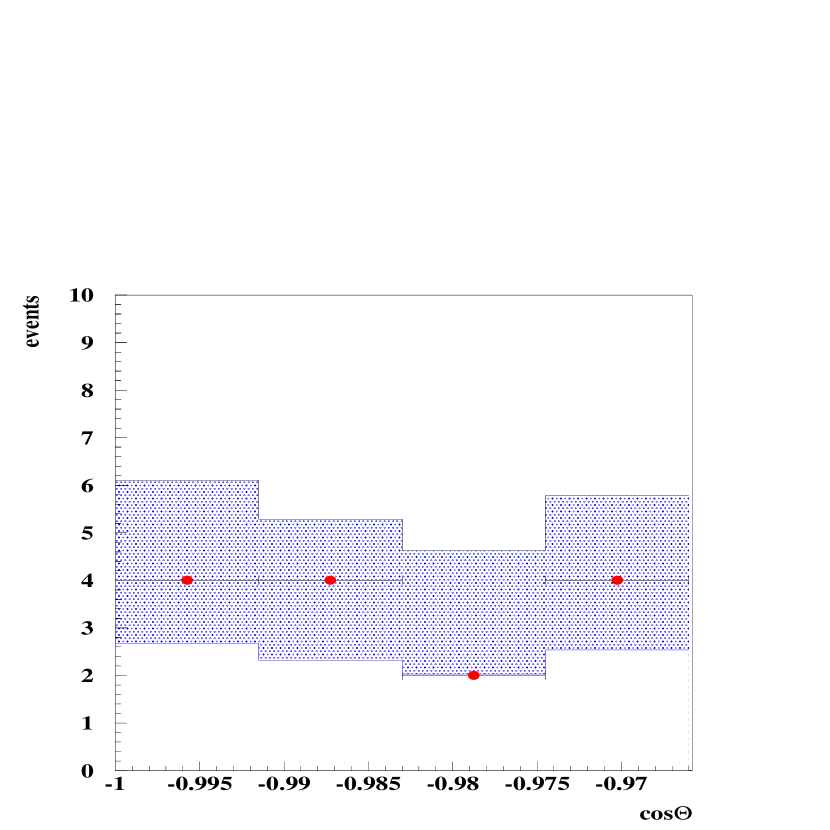
The remaining data at this level are consistent with the expected atmospheric neutrino flux. Figure 6 shows the angular distribution of the remaining 14 data events and the remaining 16.0 simulated atmospheric neutrino events. The angular range shown is for $\Theta>$ 165^∘, the region where a possible neutralino signal is expected to be concentrated. No statistically significant discrepancies are found between the expected number of events and angular distributions of the atmospheric neutrino background and the data. This result is also consistent with the results on atmospheric neutrinos presented in Ref. Amanda:01a, .

Due to the different angular shapes of the neutralino signal for different neutralino masses (see figure 6 for the two extreme cases considered), we have chosen to restrict further in angle the signal region we use to extract the limit on an excess muon flux. We use angular cones that contain 90% of the signal for a given neutralino mass. The remaining data and simulated atmospheric neutrino background events for the different angular cones used are shown in table 2. The background rejection power and signal efficiency from filter level 1 to 5 are shown in figure 4 along with the effect on the data sample.

VI Systematic uncertainties

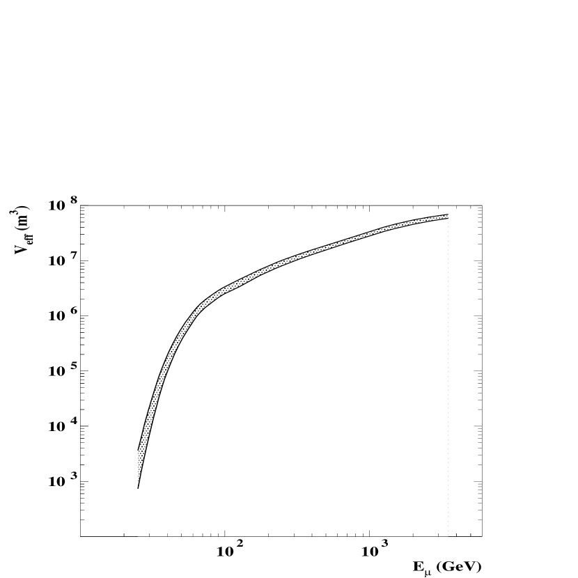
An essential quantity when deriving limits, as we do in the next section, is the effective volume, $V_{\mbox{\tiny eff}}$ , of the detector. It is the measure of the efficiency to a given signal and it is defined as

V_{\mbox{\tiny eff}}\,=\,\frac{n_{\mbox{\tiny L5}}}{n_{\mbox{\tiny gen}}}\,V_{\mbox{\tiny gen}},

(1)

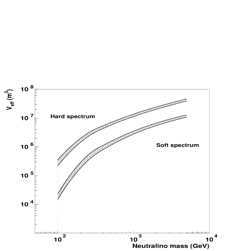
where $n_{\mbox{\tiny L5}}$ is the number of signal events after filter level 5 and $n_{\mbox{\tiny gen}}$ the number of events simulated in a volume $V_{\mbox{\tiny gen}}$ surrounding the detector. The effective volume of AMANDA-B10 as a function of muon energy is shown in figure 8. Given a MSSM model producing a muon flux with a given muon energy spectrum, the effective volume of the detector for this particular signal is also calculated through equation 1. This is shown in figure 8 for the different neutralino masses used in this analysis. The shaded bands in both figures indicate the systematic uncertainty estimated as described below.

The evaluation of $V_{\mbox{\tiny eff}}$ is subject to experimental and theoretical systematic uncertainties present in the analysis. We have performed a detailed study of the effect of the uncertainty in several variables on the resulting effective volume by propagating variations in any of them to the final evaluation of $V_{\mbox{\tiny eff}}$ .

Measurements of the scattering and absorption lengths, $\lambda_{s}$ and $\lambda_{a}$ , using pulsed and DC light sources deployed with the detector at different depths and YAG laser light sent from the surface through optical fibers, have shown that these quantities exhibit a depth dependence which is correlated with dust concentration at different levels in the ice Kurt:99a . A simulation of the detector response including layers of ice with different optical properties has been developed and used to evaluate its effect on the results. The effects introduced are muon-energy dependent and therefore dependent on the neutralino model. The effective volumes calculated with the layered ice model are reduced between 1% and 20% with respect to the uniform ice model, except for the lower neutralino mass and soft annihilation channel (100 GeV) where the effect reaches 50%.

A further correction accounts for the uncertainties in the optical modules’ total and angular sensitivities. It is known that during the process of re-freezing after deployment, air bubbles appear in the column of ice that has been melted, changing locally the scattering length of the ice and distorting the effective optical module angular sensitivity with respect to that measured in the laboratory. We have used a specific ice model for the ice in the holes that accommodates this effect. The fact that it appears after deployment and that it is not directly measurable in the laboratory makes it difficult to assess. Only by an iterative process of comparison of data and different hole-ice models can it be quantified. We estimate this effect to yield and increase of 20% in effective volume with respect to the uniform angular response model with, again, the soft annihilation channel of the lowest mass neutralino giving a stronger effect of 34%. An additional 20% uncertainty on the total optical module sensitivity has been used.

The way to combine of all these effects into a final estimate of the total uncertainty in $V_{\mbox{\tiny eff}}$ is a difficult subject, since they are not independent contributions. As described in the previous paragraphs, by varying the initial parameters used in the simulations of the detector and in the ice properties, we have obtained a range of possible values for the effective volume, which we consider as equally probable giving our current understanding of the detector. We have chosen to take the nominal $V_{\mbox{\tiny eff}}$ to be used in equation 1 as the middle value of this range. As a conservative estimate of the uncertainty we take half the width of the range of values obtained. We thus conclude that our current estimate of $V_{\mbox{\tiny eff}}$ is affected by a systematic uncertainty $\sigma_{\tiny V_{\mbox{eff}}}/V_{\mbox{\tiny eff}}$ between 10% and 25% depending on the neutralino mass considered, the lower mass of 100 GeV giving the larger relative error. A similar estimate including the same effects has been made for the atmospheric neutrino Monte Carlo. In this case we estimate the uncertainty on the effective volume for atmospheric neutrinos to be 20%.

Further uncertainty in the number of expected atmospheric neutrinos (column 3 in table 1) is caused by the uncertainties present in the calculation of the atmospheric neutrino flux. This is estimated to be of the order of 30% in the energy region relevant to this analysis, and originates mainly from uncertainties in the normalization of the primary cosmic ray spectrum and in the hadronic cross sections involved Gaisser:01a . This has been taken into account as an additional effect on top of the experimental uncertainty on the effective volume for atmospheric neutrinos, as described in section VII.2.

It has recently been shown that different muon propagation codes can produce differences in the muon flux and energy spectrum at the detector depth (see for example Ref. Sokalski:01a, ). The code used in this analysis uses the Lohmann Lohmann:85a parametrizations for muon energy loss, which produce results in agreement within about 10% of more recent codes Dima:01a for muon energies up to a few of TeV. We have not included any systematics arising from the treatment of muon propagation in the ice in this analysis.

VII Results

From the observed number of events, n ${}_{\mbox{\tiny obs}}$ , and the number of expected atmospheric neutrino background events, n ${}_{\mbox{\tiny B}}$ , an upper limit on the signal, N_β, at a chosen confidence level $\beta$ %, can be obtained. We have used the unified approach for confidence belt construction Stuart:91a to calculate 90% confidence level limits. In section B below we briefly describe a novel way of calculating limits in the presence of systematic uncertainties that we have used to obtain the final numbers presented in this paper.

Table 2: Number of data events, simulated atmospheric neutrino background events and the corresponding N

{}_{\mbox{\tiny 90}}

for the angular cones containing 90% of the signal for the different neutralino masses. These angular cuts are applied in addition to the level 5 filter described in section V. “s” and “h” denote the soft and hard annihilation channels. The numbers in parenthesis in column 5 show N

{}_{\mbox{\tiny 90}}

obtained without including systematic uncertainties.

m_χ

Angular cut

Data

Atmospheric

{}_{\mbox{\tiny 90}}

(GeV)

(deg)

(evts.)

neutrinos (evts.)

100s

167.5

12.1

9.2(4.7)

100h

168.5

10.8

6.6(4.7)

250s

170.0

8.6

5.9(4.1)

250h	$\bigg{\}}$
500s

172.0

6.1

5.6(3.9)

1000s

173.0

4.6

5.3(3.9)

500h

173.5

4.6

5.3(3.9)

1000h	$\bigg{\}}$
3000s

174.0

3.9

5.6(4.7)

3000h	$\bigg{\}}$
5000s
5000h

174.5

3.9

4.4(3.6)

VII.1 Flux limits: the standard approach

For detectors with a fixed geometrical area A, it is natural to derive a muon flux limit directly through $\phi_{\mu}\leq\mbox{N}_{\beta}/A\cdot t$ , where $t$ is the detector live-time. However, due to the large volume of AMANDA and the lack of sharp geometrical boundaries it is the effective volume $V_{\mbox{\tiny eff}}$ , as defined in equation 1, that has to be used to determine a limit on the volumetric neutrino-to-muon conversion rate, $\Gamma_{\nu\mu}$ . The effective volume provides a measure of the detector efficiency since, in addition to through-going tracks, it takes into account the effect of tracks starting or stopping within the detector. A limit can then be set on $\Gamma_{\nu\mu}$ , that is, on the number of muons with an energy above the detector threshold $E_{\mbox{\tiny thr}}$ produced by neutrino interactions per unit volume and time,

\Gamma_{\nu\mu}\,\leq\,\frac{\mbox{N}_{\mbox{\tiny 90}}}{V_{\mbox{\tiny eff}}\cdot t}

(2)

$\Gamma_{\nu\mu}$ includes all the detector threshold effects and model dependencies, as indicated below, and can be directly related to a more physically meaningful quantity, the annihilation rate, $\Gamma_{\mbox{\tiny A}}$ , of neutralinos in the center of the Earth through

Table 3: The 90

\%

confidence level upper limits on the muon flux from neutralino annihilations in the center of the Earth,

\phi_{\mu}

, for a muon energy threshold

\geq

1 GeV. The last column shows the threshold-independent neutralino annihilation rate,

\Gamma_{\mbox{\tiny A}}

. Detector systematic uncertainties have been included in the calculation of the limits. The corresponding numbers without including uncertainties are shown in parenthesis

$m_{\chi}[GeV]$	annihil.	$\phi_{\mu}$	$\Gamma_{\mbox{\tiny A}}$
	channel	$[\times 10^{3}{\rm Km^{-2}yr^{-1}}]$	$[{\rm s^{-1}}]$
100	hard	8.9 (6.3)	4.0 (2.9) $\times$ 10¹⁴
	soft	133.5 (68.2)	4.3 (2.2) $\times$ 10¹⁶
250	hard	2.1 (1.5)	1.3 (0.9) $\times$ 10¹³
	soft	6.9 (3.9)	3.8 (2.2) $\times$ 10¹⁴
500	hard	1.5 (1.1)	2.5 (1.8) $\times$ 10¹²
	soft	2.7 (1.9)	4.4 (3.0) $\times$ 10¹³
1000	hard	1.5 (1.2)	6.5 (5.4) $\times$ 10¹¹
	soft	1.8 (1.4)	9.2 (6.8) $\times$ 10¹²
3000	hard	1.1 (1.0)	7.5 (6.7) $\times$ 10¹⁰
	soft	1.5 (1.3)	1.5 (1.3) $\times$ 10¹²
5000	hard	1.1 (1.0)	3.2 (2.8) $\times$ 10¹⁰
	soft	1.5 (1.2)	7.6 (6.4) $\times$ 10¹¹

\begin{split}\Gamma_{\nu\mu}(m_{\chi})=\Gamma_{\mbox{\tiny A}}\cdot\frac{1}{4\pi R_{\oplus}^{2}}\int_{0}^{m_{\chi}}\sum B_{\chi{\bar{\chi}}\rightarrow X}\,\left(\frac{dN_{\nu}}{dE_{\nu}}\right)\,&\\ \times\,\sigma_{{}_{\nu+N\rightarrow\mu+...}}(E_{\nu}|E_{\mu}\geq E_{\mbox{\tiny thr}})\,\rho_{\mbox{\tiny N}}\,dE_{\nu},\end{split}

(3)

where the term inside the integral takes into account the production of muons through the neutrino-nucleon cross section, $\sigma_{\nu+N}$ , weighted by the different branching ratios of the $\chi{\bar{\chi}}$ annihilation process and the corresponding neutrino energy spectra, $B_{\chi{\bar{\chi}}\rightarrow X}$ $dN_{\nu}/dE_{\nu}$ . $\rho_{\mbox{\tiny N}}$ is the nucleon density of the ice and $R_{\oplus}$ is the radius of the Earth. We have used a muon energy threshold of 10 GeV in the simulations of the signal, which has been taken into account through the muon production cross section.

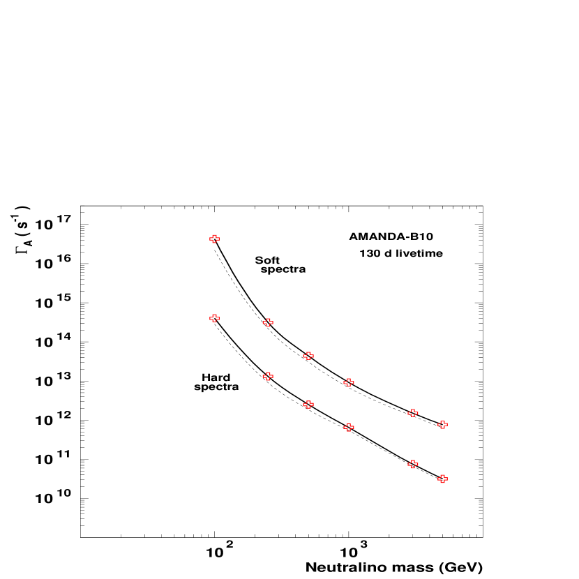
Equation 3 is solved for $\Gamma_{\mbox{\tiny A}}$ . $\Gamma_{\mbox{\tiny A}}$ depends on the MSSM model assumptions, as well as the galactic halo model used, being related to the capture rate of neutralinos in the Earth. Different neutralino models predict different capture and annihilation rates that can be probed by experimental limits set on $\Gamma_{\mbox{\tiny A}}$ . The right column of table 3 shows the limits thus derived for $\Gamma_{\mbox{\tiny A}}$ . The corresponding curves are shown in figure 10. Quoting limits on the annihilation rate has the advantage that the detector efficiency and threshold are included through equation 2 and, therefore, numbers published by different experiments are directly comparable. This is not usually the case when presenting limits on muon fluxes, where at least the detector energy threshold enters in a non trivial way and prevents direct comparison between experiments. However, since it is common in the literature to present limits on the muon flux per unit area and time, we transform below our limit on $\Gamma_{\mbox{\tiny A}}$ into a limit on the muon flux from neutralino annihilations in the center of the Earth.

The total number of muons per unit area and time above any energy threshold E ${}_{\mbox{\tiny thr}}$ within a cone of half angle $\theta_{c}$ as a function of the annihilation rate is

\phi_{\mu}(E_{\mu}\geq E_{\mbox{\tiny thr}},\theta\geq\theta_{c})\,=\,\frac{\Gamma_{\mbox{\tiny A}}}{4\pi R_{\oplus}^{2}}\int_{E_{\mbox{\tiny thr}}}^{\infty}dE_{\mu}\int_{\theta_{c}}^{\pi}d\theta\frac{d^{2}N_{\mu}}{dE_{\mu}d\theta},

(4)

where the term $d^{2}N_{\mu}/dE_{\mu}d\theta$ represents the number of muons per unit angle and energy produced from the neutralino annihilations, and includes all the MSSM model dependencies for neutrino production from neutralino annihilation and the neutrino-nucleon interaction kinematics, as well as muon energy losses from the production point to the detector. The upper limits on the annihilation rate are thus converted to a limit on the neutralino-induced muon flux at any depth and above any chosen energy threshold and angular aperture. The 90% confidence level upper limits on the annihilation rate and the muon flux at an energy threshold of 1 GeV derived using equations 2, 3 and 4 are shown in parenthesis in table 3. The fluxes have been corrected for the inefficiency introduced by using angular cones that include 90% of the signal, so the numbers presented represent the limit on the total muon flux for each neutralino model. The threshold of 1 GeV has been chosen to be able to compare with published limits by other experiments that have similar muon thresholds (see section VIII below).

VII.2 Evaluation of the limits including systematic uncertainties

However, the best limits an experiment can set are affected by the systematic uncertainties entering the analysis. Including the known theoretical and experimental systematic uncertainties in the calculation of a flux limit is not straightforward, and often overlooked in the literature. A precise evaluation of a limit should involve the incorporation of both the uncertainties in the background counts, $\sigma_{\mbox{\tiny b}}$ , and in the effective volume, $\sigma_{\mbox{\tiny V}}$ . An additional caveat arises since the uncertainty in the effective volume introduces in turn an additional uncertainty in the expected number of background events, on top of the 30% uncertainty used in the background neutrino flux $\sigma_{\mbox{\tiny b}}$ . A proper implementation of the systematics in the calculation of a limit should take this correlation into account.

One approach to incorporate systematic uncertainties into an upper limit has been proposed in Ref. Cousins:92a, . We have developed a similar method suited to our specific case which includes the systematic uncertainty in $V_{\mbox{\tiny eff}}$ in the calculation of N ${}_{\mbox{\tiny 90}}$ used in equation 2. The method is a modified Neyman-type confidence belt construction Jan:01a . The confidence belt for a desired confidence level $\beta$ is constructed in the usual way by integrating the Poisson distribution with mean n ${}_{\mbox{\tiny tot}}$ =n ${}_{\mbox{\tiny S}}$ +n ${}_{\mbox{\tiny B}}$ so as to include a $\beta$ % probability content. But the number of events for signal and background, n ${}_{\mbox{\tiny S}}$ and n ${}_{\mbox{\tiny B}}$ , are taken themselves to be random variables obtained from Gaussian distributions with means equal to the actual number of signal and background events observed and widths corresponding to the systematic uncertainties in signal and background.

Given an experimentally observed number of events, N ${}_{\mbox{\tiny exp}}$ , the 90% confidence level limit on the number of signal events is obtained by simply inverting the calculated N ${}_{\mbox{\tiny 90}}(\mbox{n}_{\mbox{\tiny tot}})$ at the corresponding n ${}_{\mbox{\tiny tot}}$ =N ${}_{\mbox{\tiny exp}}$ value. In this way the different uncertainties for signal and background and the correlation between them are included naturally.

In summary, the inclusion of our present systematic uncertainties in the flux limit calculation yields results which are weakened between $\sim$ 10% and $\sim$ 40% (practically a factor of 2 for the soft channel of m_χ=100 GeV) with respect to those obtained using N₉₀ calculated without systematics. The effect is dependent on the WIMP mass, and it reflects the better sensitivity of AMANDA for higher neutrino energies. Figures 10 and 10 show the 90% confidence level limit on the neutralino annihilation rate and the corresponding limit on the resulting muon flux for a muon threshold of 1 GeV for the hard and soft annihilation channels considered in the analysis. The symbols show the particular neutralino masses used in the simulation. The lines are to guide the eye and they show the limits obtained including systematic uncertainties (solid). The dashed lines, included for comparison, show the values obtained using the Neyman construction with the unified ordering scheme without including uncertainties. Table 3 summarizes the corresponding numbers.

VII.3 Effect of neutrino oscillations

To account for neutrino oscillations among the different flavors, the atmospheric neutrino spectrum should be weighted by a factor W(E_ν) which includes the probability that a muon neutrino has oscillated into another flavor in its way through the Earth to the detector. For the purpose of illustration consider a two-flavor oscillation scenario between $\nu_{\mu}$ and $\nu_{\tau}$ . Then W(E_ν) = $1-\mbox{sin}^{2}(2\theta)\,\mbox{sin}^{2}\left(1.27\,\Delta\mbox{m}^{2}[\mbox{eV}^{2}]\,\mbox{D}_{\oplus}[\mbox{km}]/\mbox{E}_{\nu}[\mbox{GeV}]\right)$ , where $\mbox{D}_{\oplus}$ is the diameter of the Earth, $\theta$ the mixing angle and $\Delta\mbox{m}^{2}$ the difference of the squares of the flavor masses. Note that the effect depends strongly on the neutrino energy and it is negligible in the high energy tail of the atmospheric spectrum since the oscillation length is then much larger than the Earth diameter. If we choose $\mbox{sin}^{2}(2\theta)$ =1 and $\Delta\mbox{m}^{2}=2.5\times 10^{-3}$ eV² based on the results obtained in Ref. Kameda:01a, , the number of expected atmospheric neutrino events is reduced between 5% and 10%, depending on the angular cone considered. This would weaken the limits by about the same amount.

The effect of neutrino oscillations on the possible WIMP signal is model dependent and has been estimated in Refs. Marek:01a, and Fornengo:00a, . However the authors reach different conclusions on the direction of the effect: up to a factor of two in increased muon flux in Ref. Marek:01a, and a reduction of about 25% in Ref. Fornengo:00a, for a neutralino mass of 100 GeV. For higher neutralino masses both authors predict a less pronounced effect, which becomes negligible for the higher masses considered in Marek:01a (m ${}_{\chi}>$ 300 GeV). We have not included any oscillation effect on the neutrinos from the WIMP signals considered in this paper.

VIII Comparison with other experiments and theoretical models

Searches for a neutrino signal from WIMP annihilation in the center of the Earth have been performed by MACRO, Baikal, Baksan, and Super-Kamiokande.

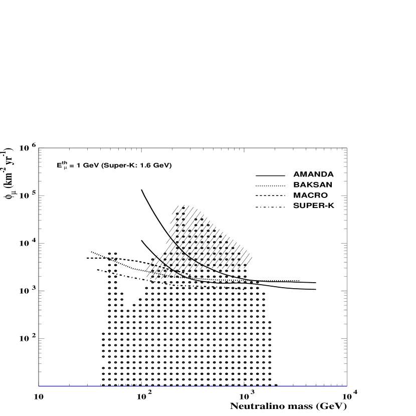
In figure 11 the results of Baksan Boliev:97a , MACRO Ambrosio:99a and Super-Kamiokande Habig:01a are shown along with the limits from AMANDA obtained in the previous section and theoretical predictions of the MSSM as a function of WIMP mass. In order to be able to compare with the other experiments, the Super-Kamiokande limits have been scaled by a factor 1/0.9 to represent total flux limits, instead of limits based on angular cones including 90% of the signal as originally presented in Ref. Habig:01a, . The 90% confidence level muon flux limits for a muon energy threshold of 10 GeV published by the Baikal collaboration range between 0.63 $\times$ 10⁴ km^-2 yr^-1 for a zenith half cone of 15^∘ and 0.54 $\times$ 10⁴ km^-2 yr^-1 for a zenith half cone of 5^∘ (Ref. Balkanov:99a, ). Since these results are not presented as a function of WIMP mass, and are quoted at a slightly higher muon energy threshold, we have not included them in the figure but we mention them here for completeness.

Each point in the figure represents a flux obtained with a particular combination of MSSM parameters, following Ref. Bergstrom:98b, . The sixty four original free parameters of the general MSSM have been reduced to seven by the standard assumptions about the behavior of the theory at the GUT scale and about the supersymmetry breaking parameters in the s-fermion sector. The independent parameters left are the Higgsino mass parameter $\mu$ , the ratio of the Higgs vacuum expectation values tan $\beta$ , the gaugino mass parameter M ${}_{\mbox{\tiny 2}}$ , the mass m ${}_{\mbox{\tiny A}}$ of the CP-odd Higgs boson and the quantities m ${}_{\mbox{\tiny o}}$ , A ${}_{\mbox{\tiny t}}$ and A ${}_{\mbox{\tiny b}}$ from the ansatz on the scale of supersymmetry breaking. These parameters were varied in the following ranges: -5000 $\leq\mu\leq$ 5000 GeV , -5000 $\leq{\mbox{M}_{\mbox{\tiny 2}}}\leq$ 5000 GeV, 1.2 $\leq\mbox{tan}\beta\leq$ 50, m ${}_{\mbox{\tiny A}}\leq$ 1000 GeV, 100 $\leq\mbox{m}_{\mbox{\tiny o}}\leq$ 3000 GeV, -3m ${}_{\mbox{\tiny o}}\leq{\mbox{A}}_{\mbox{\tiny b}}\leq$ 3m ${}_{\mbox{\tiny o}}$ and -3m ${}_{\mbox{\tiny o}}\leq\mbox{A}_{\mbox{\tiny t}}\leq$ 3m ${}_{\mbox{\tiny o}}$ . Models based on parameters already excluded by accelerator limits are not shown, and the figure is restricted to those models which give cosmologically interesting neutralino relic densities, 0.025 $\lesssim\Omega_{\chi}h^{2}<$ 0.5. A local dark matter density of 0.3 GeV/cm³ has been assumed. Theoretical predictions for high mass neutralino models lie below the scale of the plot, since in this case the number density of neutralinos falls down rapidly if the dark matter density is kept fixed.

A complementary way to search for neutralinos is by measuring the nuclear recoil in elastic neutralino-nucleus collisions on an adequate target material Jungman:96a . Experiments using this direct detection technique set limits on the neutralino-nucleon cross section as a function of neutralino mass. The same scan over MSSM parameter space used to generate the theoretical points in figure 11 can be used to identify parameter combinations that are accessible by direct searches. There is not, however, a one-to-one correspondence between the results of the direct detection searches and the expected neutrino flux from the models probed, so comparisons with the results of indirect searches have to be performed with care. We have indicated the models disfavored by the DAMA collaboration Bergstrom:98c by the dashed area in the figure, which has to be taken as an approximate region in view of the mentioned difficulties in comparing both types of detection techniques. We note that the models that yield high muon fluxes, and that are disfavored by both current results from direct searches and by the limits shown in the figure, have in common a low value of the H ${}^{0}_{2}$ mass, around 92 GeV.

IX Summary

We have performed a search for a statistically significant excess of vertically up-going muons with the AMANDA neutrino detector as a signature for neutralino annihilation in the center of the Earth. Limits on the neutralino annihilation rate have been derived from the non-observation of a signal excess over the predicted atmospheric neutrino background. We have included the effect of the detector systematic uncertainties and the theoretical uncertainty in the expected number of background events in the derivation of the limits, presenting in this way realistic limit values.

A comparison with the results of MACRO, Super-K and Baksan, as well as with theoretical expectations from the MSSM are presented. AMANDA, with only 130.1 days of effective exposure in 1997, has reached a sensitivity in the high neutralino mass ( $>$ 500 GeV) region comparable to that achieved by detectors with much longer live-times.

Acknowledgements.

AMANDA is supported by the following agencies: The U.S. National Science Foundation, the University of Wisconsin Alumni Research Foundation, the U.S. Department of Energy, the U.S. National Energy Research Scientific Computing Center, the Swedish Research Council, the Swedish Polar Research Council, the Knut and Allice Wallenberg Foundation (Sweden) and the German Federal Ministry of Education and Research. D. F. Cowen acknowledges the support of the NSF CAREER program. C.P. de los Heros acknowledges support from the EU 4

{}^{\mbox{\tiny th}}

framework of Training and Mobility of Researches. P. Loaiza was supported by the Swedish STINT programme. We acknowledge the invaluable support of the Amundsen-Scott South Pole station personnel. We are thankful to I.F.M. Albuquerque and W. Chinowsky for their careful reading of the manuscript and valuable comments.

References

(1) L. Bergström. Rep. Prog. Phys. 63, 793 (2000).
(2) G. Jungman, M. Kamionkowski and K. Griest. Phys. Rep. 267, 195 (1996).
(3) K. Griest and M. Kamionkowski. Phys. Rev. Lett. 64, 615 (1990).
(4) G. Abbiendi et al. Eur. Phys. Jour. C, 14, 2, 187 (2000).
(5) J. Edsjö and P. Gondolo. Phys. Rev. D56, 1879 (1997).
(6) W. H. Press, D. N. Spergel, Astrophys. J. 296, 769 (1985).
(7) K. Freese. Phys. Lett. B167, 295 (1986); T. Gaisser, G. Steigman, S. Tilav, Phys. Rev. D34, 2206 (1986).
(8) A. Gould, Ap. J. 328, 919, (1988).
(9) J. L. Feng, K. T. Matchev and F. Wilczek. Phys. Rev. D63, 045024 (2001).
(10) E. Andrés et al. Astropart. Phys., 13, 1 (2000).
(11) E. Andrés et al. Nature 410 (2001); Ch. Wiebusch et al. Proceedings of the XVII International Cosmic Ray Conference (ICRC), Hamburg, Germany, 2001, p. 1109; J. Ahrens et al. Submitted to Phys. Rev. D. astro-ph/0205109.
(12) R. Wischnewski et al. Proceedings of the XVII International Cosmic Ray Conference (ICRC), Hamburg, Germany, p. 1105; S. Barwick et al. ibi. p. 1101.
(13) J. Edsjö, PhD. Thesis. Uppsala University, 1997. hep-ph/9704384. L. Bergström, J. Edsjö and P. Gondolo. Phys. Rev. D58, 103519 (1998).
(14) T. Sjöstrand. Comp. Phys. Comm. 82, 74 (1994).
(15) P. Lipari. Astropart. Phys., 1, 195 (1993).
(16) R. Ghandi et al. Astropart. Phys., 5, 81 (1996).
(17) H. L. Lai et al. Phys. Rev. D51, 1280 (1995).
(18) E. Dalberg, PhD Thesis. Stockholm University, 1999. ISBN 91-7265-024-9.
(19) S. N. Boziev et al. INR preprint P-0630, Moscow (1989).
(20) T. K. Gaisser. Cosmic Rays and Particle Physics. Cambridge Univ. Press (1990).
(21) D. Heck et al.. FZKA report 6019 (1998). http://ik1au1.fzk.de/~heck/corsika/
(22) Particle Data Group, Eur. Phys. Jour. 15, 1-4 (2000).
(23) W. Lohmann et al. CERN Yellow Report CERN-EP/85-03. (1985).
(24) G. Hill et al. in Proceedings of the XVI International Cosmic Ray Conference (ICRC), Salt Lake City, Utah, USA, 1999. HE.6.3.02.
(25) V. J. Stenger, University of Hawaii preprint, HDC-1-90 (1990)
(26) C. Wiebusch. Proceedings of the International Workshop on Simulations and Analysis Methods for Large Neutrino Telescopes, Zeuthen, Germany, 1998, edited by C. Spiering (DESY-PROC-1999-01, 1999), p. 302.
(27) P. Loaiza, Licentiat thesis. Uppsala University, 2000.
(28) T. G. M. Malmgren. Comm. Phys. Comm. 106, 230 (1997).
(29) K. Woschnagg, in Proceedings of the XVI International Cosmic Ray Conference (ICRC), Salt Lake City, Utah, USA, 1999. HE.4.1.15.
(30) T. Gaisser et al. Proceedings of the XVII International Cosmic Ray Conference (ICRC), Hamburg, Germany, 2001, p. 1643.
(31) I. Sokalski et al. Phys. Rev. D64, 074015 (2001).
(32) D. Chirkin and W. Rhode. Proceedings of the XVII International Cosmic Ray Conference (ICRC), Hamburg, Germany, 2001, p. 1017.
(33) A. Stuart, J. K. Ord. Kendall’s Advanced Theory of Statistics, Vol. 2. Oxford Univ. Press, (1991); G. J. Feldman and R. D. Cousins, Phys. Rev. D57, 873 (1998).
(34) R. D. Cousins, V. L. Highland, Nucl. Instr. Meth. A320, 331 (1992).
(35) J. Conrad et al. Proceedings of the workshop on Advanced Statistical Techniques in Particle Physics, Durham, UK, 2002; hep-ex/0202013.
(36) J. Kameda et al. Proceedings of the XVII International Cosmic Ray Conference (ICRC), Hamburg, Germany, 2001, p. 1057.
(37) M. Kowalski. Phys. Lett. B511, 119, (2001).
(38) N. Fornengo. Proceedings of the Third International Conference on Dark Matter in Astro and Particle Physics, Heidelberg, Germany, 2000. Also hep-ph/0011030.
(39) P. Gondolo et al. Proceedings of the Third International Workshop on Identification of Dark Matter (IDM2000), York, UK, 2000, edited by N. J. C. Spooner and V. Kudryavtsev (World Scientific, 2001), p. 318. astro-ph/0012234; http://www.physto.se/~edsjo/darksusy/
(40) M. Boliev et al.. Proceedings of Dark Matter in Astro and Particle Physics, 1997. H. V. Klapdor-Kleingrothaus and Y. Ramachers, eds., (Worl Scientific, Singapore, 1997), p. 711. See also O. Suvorova, hep-ph/9911415.
(41) M. Ambrosio et al. Phys. Rev. D60, 082002 (1999).
(42) A. Habig et al. Proceedings of the XVII International Cosmic Ray Conference (ICRC), Hamburg, Germany, 2001, p. 1558. Also hep-ex/0106024.
(43) V. A. Balkanov et al. Proceedings of Neutrino 2000, Sudbury, Canada, 2000. Nucl. Phys. B91, 438 (2001).
(44) L. Bergström, J. Edsjö and P. Gondolo. Phys. Rev. D55, 1765 (1997).
(45) L. Bergström, J. Edsjö and P. Gondolo. Phys. Rev. D58, 103519 (1998).