Lensing of ultra-high energy cosmic rays
in turbulent magnetic fields

Abstract:

We consider the propagation of ultra high energy cosmic rays through turbulent magnetic fields and study the transition between the regimes of single and multiple images of point-like sources. The transition occurs at energies around $E_{c}\simeq Z~{}41\ {\rm EeV}(B_{rms}/5\ \mu{\rm G})\left(L/2~{}{\rm kpc}\right)^{3/2}\sqrt{50~{}{\rm pc}/L_{c}}$, where $L$ is the distance traversed by the CR’s with electric charge $Ze$ in the turbulent magnetic field of root mean square strength $B_{rms}$ and coherence length $L_{c}$. We find that above $2E_{c}$ only sources located in a fraction of a few % of the sky can reach large amplifications of its principal image or start developing multiple images. New images appear in pairs with huge magnifications, and they remain amplified over a significant range of energies. At decreasing energies the fraction of the sky in which sources can develop multiple images increases, reaching about 50% for $E>E_{c}/2$. The magnification peaks become however increasingly narrower and for $E<E_{c}/3$ their integrated effect becomes less noticeable. If a uniform magnetic field component is also present it would further narrow down the peaks, shrinking the energy range in which they can be relevant. Below $E\simeq E_{c}/10$ some kind of scintillation regime is reached, where many demagnified images of a source are present but with overall total magnification of order unity. We also search for lensing signatures in the AGASA data studying two-dimensional correlations in angle and energy and find some interesting hints.

1 Introduction

One of the fundamental open problems in physics is to understand the nature and origin of the ultra-high energy cosmic rays (UHECRs). The increased aperture of the next generation of CR detectors (e.g. the Auger Observatory) will be crucial to attempt to locate possible astrophysical point-like sources from the observation of clustering or anisotropies in the arrival directions. If the UHECRs are electrically charged, as would be the case in the likely situation that they are protons or heavier nuclei, a very important fact which has to be taken into account is their deflection by the magnetic fields present along their path. These deflections are expected to be quite large below the ankle (i.e. for $E<5\times 10^{18}$ eV), and hence no CR ‘astronomy’ is possible below those energies since the information about the original source direction cannot be recovered from the observed arrival directions. On the other hand, since typical galactic magnetic fields ($B\simeq{\rm few}\ \mu$G) are unable to confine CRs within the Galaxy for energies above the ankle, this supports the belief that UHECRs have an extragalactic origin, in agreement with the absence of strong anisotropies toward the Galactic disk being observed at those energies. The decreasing magnetic deflections for increasing energies lend us hope that a correlation among the arrival directions of different CR events and between those and the possible source directions will clearly show up with increased statistics at energies $E\gg 10^{19}$ eV, when the CR trajectories progressively approach the rectilinear propagation regime.

The astrophysical magnetic fields [1, 2, 3] may be classified under two broad categories: the regular and the random fields. Large scale regular fields may be produced by adiabatic compression of preexisting cosmic seed fields, by their amplification by a dynamo mechanism or may be related to the action of a galactic wind. They are known to exist in our galaxy (and other spirals as well), where the field lines essentially follow the spiral structure, with reversals in direction taking place between neighboring arms. The existence of coherent fields in the halo or even larger scales is debatable, as is the presence of regular fields on cluster scales. The random component is present on galactic scales, probably originating from supernova explosions which feed power on typical scales of $\sim 100$ pc, which is latter transferred to smaller scales due to the turbulence present in the high Reynold’s number interstellar medium. This leads to a Kolmogorov spectrum of magnetic field fluctuations extending probably down to very small scales ($\sim 10^{8}$ m [4]) and with an rms amplitude exceeding the typical values of the uniform field by a factor $2\div 3$. In cluster’s cores $\mu$G fields have been observed, and their coherence length is believed to be at the kpc scale. For the intergalactic medium usually turbulent random fields are also assumed to exist, but with much larger coherence lengths ($\sim 1$ Mpc). The amplitude of these fields is bounded from the non-observation of Faraday rotation of distant polarized radio sources, but it can be sizeable ($\sim 10^{-8}\div 10^{-7}$ G) if confined in thick sheets e.g. around the supergalactic plane.

The existence of these magnetic fields will certainly affect the observable properties of UHECRs (see e.g. [5, 6, 7, 8, 9, 10]). As we have shown in previous works [11, 12], besides inducing a change in the arrival directions, the deflections caused by the magnetic fields can also lead to strong lensing phenomena, including the formation of multiple images and energy dependent magnifications or demagnifications of the CR fluxes. In those works we dealt with the effects resulting from the regular galactic magnetic field, which were shown to lead to important consequences for $E/Z<30$ EeV (where $Ze$ is the assumed CR charge and $1~{}{\rm EeV}\equiv 10^{18}$ eV). It is the purpose of the present work to extend the analysis of the magnetic lensing effects to the case of random magnetic fields, and consider also the possible interplay between the random and uniform components.

One may distinguish between four different energy regimes when CRs traverse a distance $L$ through a random field with coherence length $L_{c}$. If $\delta\propto 1/E$ is the typical deflection suffered by the CRs, in the high energy limit, corresponding to $\delta\ll L_{c}/L$, CRs propagate almost rectilinearly and those arriving to an observer from a faraway source have all seen essentially the same magnetic field. When $\delta\sim L_{c}/L$, we enter the regime in which multiple images of the same source can appear and CRs from different images have felt uncorrelated values of the magnetic field. We find that in this regime large magnification effects may be observable. For $\delta>{\rm few}L_{c}/L$, a regime with large quantities of secondary images appears, having the property that magnification effects tend to be averaged out, and essentially only a blurred image with characteristic angular size given by $\delta$ will be observable. The fourth regime is that of spatial diffusion of the CRs, which is established when the gyroradius of the CRs is smaller than $L_{c}$. For instance, for the galactic magnetic fields this happens below the ankle (for $E/Z<0.3$ EeV), but may happen at much larger energies for UHECRs propagating across intergalactic magnetic fields. The energy dependence of the associated diffusion coefficients in this regime can lead to important changes in the slope of the CR spectrum, as is known to be the case for galactic CRs below the ankle.

We will focus our work here in the systematic study of the first three regimes just described. Let us mention that focusing effects produced by random fields were previously noticed in the numerical study of ref. [10], but were not analyzed in detail, while the first and third regimes were considered in refs. [7] in relation to the study of the time delays associated to bursting sources.

2 The turbulent field

We model the turbulent magnetic field as a Gaussian random field with zero mean and root mean square value $B_{rms}$. This can be described by a superposition of Fourier modes as

$$B_{i}({\bf x})=\int\frac{{\rm d}^{3}k}{(2\pi)^{3}}B_{i}({\bf k})e^{i(\bf{k}\cdot{\bf x}+\phi_{i}({\bf k}))}~{},$$ (1)

where the phases $\phi_{i}({\bf k})$ are random. If the turbulence is isotropic and homogeneous, the random Fourier modes satisfy the relation

$$\langle B_{i}({\bf k})B_{j}({\bf k^{\prime}})\rangle={B^{2}(k)\over 8\pi k^{2}}P_{ij}(2\pi)^{6}\delta({\bf k}+{\bf k^{\prime}})~{},$$ (2)

where the projection tensor $P_{ij}=\delta_{ij}-{k_{i}k_{j}/k^{2}}$ guarantees that the field is solenoidal (${\bf\nabla}\cdot{\bf B}=0$) [13]. We will consider the general case of a power spectrum

$$B^{2}(k)=B_{rms}^{2}k^{-n}{(n-1)(2\pi/L_{max})^{n-1}\over 1-(L_{min}/L_{max})^{n-1}}~{},$$ (3)

for $2\pi/L_{max}\leq k\leq 2\pi/L_{min}$, and zero otherwise. This power spectrum is already normalized such that $\langle|{\bf B}({\bf x})|^{2}\rangle=B_{rms}^{2}$. The particularly interesting case of a Kolmogorov spectrum (for which the energy density d$E/{\rm d}k\propto k^{-5/3}$) corresponds to a spectral index $n=5/3$.

The correlation length of this field, $L_{c}$, can be defined through

$$\int_{-\infty}^{\infty}{\rm d}L\langle{\bf B}(0)\cdot{\bf B}({\bf x}(L))\rangle\equiv L_{c}B_{rms}^{2}~{},$$ (4)

where the point ${\bf x}(L)$ is displaced with respect to the origin by a distance $L$ along a fixed direction. The integral in the lhs of Eq. (4) can be computed using Eqs. (1) and (2), and leads to

$$\pi\int_{0}^{\infty}{{\rm d}k\over k}B^{2}(k)=L_{c}B_{rms}^{2}$$ (5)

which can be used to express $L_{c}$ in terms of $L_{min}$ and $L_{max}$ as

$$L_{c}={1\over 2}L_{max}{n-1\over n}{1-(L_{min}/L_{max})^{n}\over 1-(L_{min}/L_{max})^{n-1}}$$ (6)

In the case of either a very sharp $(n\gg 1)$ or of a very narrow-band $(L_{min}\sim L_{max})$ spectrum, one gets $L_{c}\simeq L_{max}/2$, while for a broad-band $(L_{max}\gg L_{min})$ Kolmogorov $(n=5/3)$ spectrum, one gets instead $L_{c}\simeq L_{max}/5$.

The deflection in the velocity of a particle of charge $Ze$ travelling a distance $L$ through a magnetic field ${\bf B}$, in the limit of small deflections, can be approximated by

$$\delta=\frac{Ze}{E}\left|\int_{0}^{L}{\rm d}{\bf s}\times{\bf B}(s)\right|.$$ (7)

For particles moving in a turbulent field the mean deflection vanishes. The relevant quantity is the root mean square value

$$\delta_{rms}^{2}=\langle\delta^{2}\rangle=\left(\frac{Ze}{E}\right)^{2}\int_{0}^{L}{\rm d}s\int_{0}^{L}{\rm d}s^{\prime}\langle{\bf B}_{\perp}(s)\cdot{\bf B}_{\perp}(s^{\prime})\rangle,$$ (8)

where ${\bf B}_{\perp}(s)$ stands for the component of ${\bf B}$ in the direction orthogonal to the trajectory. This can be computed with the help of Eqs. (1)–(3). In the limit of $L\gg L_{max}$, corresponding to the distance travelled much larger than the maximum turbulence scale, the result can be written as

$$\delta_{rms}={\frac{1}{\sqrt{2}}}\frac{Ze}{E}B_{rms}\sqrt{LL_{c}}\simeq 1.5^{\circ}\frac{\rm{40~{}EeV}}{E/Z}\frac{B_{rms}}{5~{}\mu{\rm G}}\sqrt{\frac{L}{2~{}\rm{kpc}}}\sqrt{\frac{L_{c}}{50~{}{\rm pc}}}~{},$$ (9)

where we have used Eq. (5) to write it in terms of the coherence length. We have chosen to express its numerical value in terms of parameters relevant for the galactic magnetic field, which has a random component with rms strength of a few $\mu$G and a maximum scale of turbulence of order 100 pc.

Notice that the position at which the charged particle arrives forms an angle with respect to its initial velocity given by

$${\bf\eta}=\frac{Ze}{E}\left|\int_{0}^{L}{\rm d}s\int_{0}^{s}{\rm d}s^{\prime}{\bf B}_{\perp}(s^{\prime})\right|,$$ (10)

which has a root mean square value

$$\eta_{rms}=\frac{1}{\sqrt{3}}\delta_{rms}~{},$$ (11)

meaning that after traversing a distance $L$ in a turbulent field, the dispersion in the directions of the velocity vector is larger than that in the position vector as seen from the departure point by a factor $\sqrt{3}$.

3 The high energy regime

As a beam of charged particles propagates through a magnetic field, its flux is focused or defocused due to the differential deflections of neighboring paths, with the effect being larger at smaller energies. Eventually, the focusing effects may become sufficiently strong to produce multiple images of single CR sources. Heuristically, multiple images of a single source require CRs to reach from the source to their destination point traveling through uncorrelated values of the intervening magnetic field [7]. Consider a very distant source, so that its flux can be approximated as a beam of parallel CRs when they enter the region permeated by the magnetic field. The typical condition for the formation of multiple images is that two initially parallel paths separated by a distance of order $L_{c}$ may reach the same point after traversing a distance $L$ in the magnetic field, i.e. that $\eta(L)\simeq{L_{c}/2L}$, or equivalently ${\delta L}/{L_{c}}\simeq{\sqrt{3}/2}$. Multiple images of a single CR source are thus a likely possibilty at energies $E\simeq\frac{2}{\sqrt{3}}E_{c}$, with $E_{c}$ defined through

$$\delta_{rms}\equiv\frac{E_{c}}{E}\frac{L_{c}}{L}~{}.$$ (12)

Its numerical value reads

$$E_{c}\simeq Z~{}41\ {\rm EeV}\frac{B_{rms}}{5\ \mu{\rm G}}\left(\frac{L}{\rm 2\ kpc}\right)^{3/2}\sqrt{\frac{50~{}{\rm pc}}{L_{c}}}.$$ (13)

Notice that the heuristic argument above applies if the magnetic field has one dominant length scale only. If the turbulent field has a broad-band spectrum, this heuristic argument should be applied to the effect of each individual wavelength bin. Small wavelengths can actually lead to multiple image formation at higher energies than long ones if the amplitudes of the Fourier modes of the magnetic field do not decrease too fast at small scales, as will be discussed further below.

A detailed study of the focusing effects of the magnetic field can be performed following the trajectories of neighboring paths in a beam. The amplification of the flux of a CR source, given by the relative change in the area of the cross section of an initially parallel beam, can be written borrowing the formalism familiar from gravitational lensing [14] as

$$A=\frac{1}{|(1-\kappa)^{2}-\gamma^{2}|}~{}.$$ (14)

Here the convergence $\kappa$ describes the isotropic (de)focusing effect while $\gamma$ is the shear that distorts the shape of the cross section of the beam. It is useful to decompose the amplification along a particular direction of observation as $A=A_{1}A_{2}$, with $A_{1}\equiv 1/(1-\kappa-\gamma)$ and $A_{2}\equiv 1/(1-\kappa+\gamma)$ measuring the relative stretching of the beam along the so-called shear principal axes. This means that a beam with an initially circular cross section with diameter $L_{0}$ develops an elliptical cross section, with one of the principal axes having its length changed by $\Delta L_{1}=L_{0}(-\kappa-\gamma)$ and the other one by $\Delta L_{2}=L_{0}(-\kappa+\gamma)$. As the deflections due to the random field have no preferred direction, this means that $\langle\Delta L_{1}\rangle=\langle\Delta L_{2}\rangle=0$ and $\langle\Delta L_{1}^{2}\rangle=\langle\Delta L_{2}^{2}\rangle$. Since $\kappa(\gamma)\simeq-[\Delta L_{1}+(-)\Delta L_{2}]/2L_{0}$, it is then easy to see that $\langle\kappa\rangle=\langle\gamma\rangle=0$ and that $\langle\kappa^{2}\rangle=\langle\gamma^{2}\rangle$.

In the limit of small deflections the isotropic focusing of an initially parallel beam of CRs is given by [11]

$$\kappa=\frac{1}{2}\frac{Ze}{E}\int_{0}^{L}(L-s){\bf\nabla}\times{\bf B}_{\cdot}{\rm d}{\bf s}~{}.$$ (15)

Using eqs. (1)–(3) we can calculate $\langle\kappa^{2}\rangle\equiv\kappa_{rms}^{2}$, with the result

$$\kappa_{rms}=\zeta\frac{1}{\sqrt{2}}\frac{Ze}{E}B_{rms}\frac{L^{3/2}}{\sqrt{L_{c}}}=\zeta\frac{\delta_{rms}L}{L_{c}}=\zeta\frac{E_{c}}{E}~{},$$ (16)

where we defined the numerical coefficient $\zeta$ such that

$$\zeta^{2}\equiv\frac{\pi^{2}}{12}\left(\left(\frac{L_{max}}{L_{min}}\right)^{2-n}-1\right)\frac{(n-1)^{2}}{n(2-n)}\frac{1-(L_{min}/L_{max})^{n}}{(1-(L_{min}/L_{max})^{n-1})^{2}}~{}.$$ (17)

In the case of either a very sharp or of a very narrow-band spectrum, one gets $\zeta=\pi/\sqrt{12}\approx 0.9$. For a broad-band Kolmogorov spectrum, one gets instead $\zeta\approx 0.8~{}(L_{max}/L_{min})^{1/6}$. Notice that, contrary to the case of deflections, small wavelengths have a significant effect upon focusing of charged particles for spectral indices $n<2$. Indeed, if $n<2$ the energy at which $\kappa_{rms}$ becomes of order unity, and thus strong lensing effects become very likely, increases by a factor of order $\left({L_{max}}/{L_{min}}\right)^{1-n/2}$ compared to the case of a very sharp spectrum.

In the high energy regime, i.e. for $E>\zeta~{}E_{c}$, $\kappa$ and $\gamma$ are small and they can be approximated by uncorrelated random Gaussian variables with zero mean (see Eq. (15) and take into account the fact that ${\bf B}$ is Gaussian) and dispersion $\kappa_{rms}$. The probability distribution of the amplification of the beam in different observing directions, assuming that the observer is located at the center of a sphere of radius $L$ filled with a random field of constant strength $B_{rms}$ is then given by

$${{\rm d^{2}}p\over{\rm d}\kappa{\rm d}\gamma}=G_{\kappa}(0,\kappa_{rms})G_{\gamma}(0,\kappa_{rms}),$$ (18)

with $G_{x}(\bar{x},\sigma)=\exp[(x-\bar{x})^{2}/2\sigma^{2}]/\sqrt{2\pi}\sigma$.

More interesting is to study the probability $p_{s}$ that the flux from a distant source be seen by the observer with a given magnification. As long as we can neglect the presence of multiple images, which is a reasonable approximation for $E>2E_{c}$, this one is related to the probability in Eq. (18) by a factor $1/A$, since the magnification is just the ratio between the observed solid angle to that actually subtended by the source (because the surface brightness is conserved). Hence, one has that in the high energy domain

$${{\rm d^{2}}p_{s}\over{\rm d}\kappa{\rm d}\gamma}\simeq{{\rm d^{2}}p\over{\rm d}\kappa{\rm d}\gamma}|(1-\kappa)^{2}-\gamma^{2}|.$$ (19)

One can then compute the probability that a source be magnified above a certain threshold $A_{0}$ as

$$P_{s}(A>A_{0})\simeq\int\limits_{-\infty}^{\infty}{\rm d}\gamma\int\limits_{1-\sqrt{A_{0}^{-1}+\gamma^{2}}}^{1+\sqrt{A_{0}^{-1}+\gamma^{2}}}{\rm d}\kappa{{\rm d^{2}}p_{s}\over{\rm d}\kappa{\rm d}\gamma}.$$ (20)

This gives that e.g. for $E=3E_{c}$ around 6% of the source directions are magnified by a factor larger than $A_{0}=2$, while only 1% are magnified by more than a factor of five.

Figure 1: Fraction of the source directions for which multiple images would appear vs. $E/E_{c}$.

The flux from a CR source diverges after traversing a distance $L$ in the magnetic field for those directions such that $(1-\kappa-\gamma)(1-\kappa+\gamma)=0$. In that case, the source is located on top of a caustic of the magnetic field configuration relative to the specific point of observation. Multiple images of a given source are visible at energies below that at which a caustic crosses the source location. The additional images exist in pairs of opposite parity, and for the inverted image one has that $(1-\kappa)^{2}-\gamma^{2}$ is negative. We can then compute the probability that a given source has multiple images as

$$P_{mult}=P_{s}(|1-\kappa|<|\gamma|)=2\int\limits_{0}^{\infty}{\rm d}\gamma\int\limits_{1-\gamma}^{1+\gamma}{\rm d}\kappa{{\rm d^{2}}p_{s}\over{\rm d}\kappa{\rm d}\gamma}.$$ (21)

It has to be noticed that this expression is reasonably accurate as long as the fraction of sources with more than three images is negligible (which corresponds to approximately $P_{mult}<25\%$). The result is plotted in Figure 1, and we see that for $E\simeq 2E_{c}$ around 3% of the sources will have multiple images and this fraction rises to $\sim~{}20\%$ at $E\simeq 1.25E_{c}$.

Figure 2: Mean number of images of a source vs. $E/E_{c}$.

For decreasing energies, the number of images associated to a source increases. As will be shown later on in Section 6 (see Eq. (46)), this number can be computed as the mean of $A^{-1}$ over all the observing directions $\theta$. Taking the mean over many independent directions is actually equivalent to take the mean over realizations of the random field, i.e. over different values of $\kappa$ and $\gamma$. We then obtain

$$\langle n\rangle=\frac{1}{4\pi}\int{\rm d}^{2}\theta A^{-1}=\int{\rm d}\kappa{\rm d}\gamma\frac{{\rm d}^{2}p}{{\rm d}\kappa{\rm d}\gamma}|(1-\kappa)^{2}-\gamma^{2}|.$$ (22)

This expression is plotted in Figure 2 as a function of $E/E_{c}$. We see that $\langle n\rangle$ takes values 1.06, 1.8 and 4.8 for $E/E_{c}=2$, 1 and 1/2, showing that multiple imaging is of paramount importance for $E<2\ E_{c}$.

4 Numerical results

We have implemented a numerical code to propagate charged particles within a realization of a random magnetic field, obtained as the superposition of $N$ independent waves, with random directions of the vector ${\bf k}$ and direction of ${\bf B}({\bf k})$ randomly chosen in the plane orthogonal to ${\bf k}$, so that the condition ${\bf\nabla}\cdot{\bf B}=0$ is automatically fulfilled. The modulus of each mode $|{\bf B}({\bf k})|$ is drawn from a Gaussian distribution with zero mean and dispersion given by Eq. (3) with $n=5/3$ (Kolmogorov spectrum). The code allows to calculate not just deflections of trajectories but also flux amplification along them, by following two additional nearby particles, using the formalism developed in ref. [11]. In practice, CR trajectories that reach the Earth are found backtracking trajectories of particles with opposite charge from the Earth out to a sphere of radius $L$.

The code results agree with the analytic expressions in Eqs. (9) and (16) for the rms deflections and amplifications in the small deflection limit for a wide range of parameters.

A useful way to visualise the lensing properties of a magnetic field is to plot, for a regular grid of CR arrival directions on Earth, the incoming directions they had as they entered the region permeated by the field. These ‘sky sheets’ [11] are quite smooth, regular and single-valued at energies $E\gg\zeta E_{c}$, meaning that only one image of each source is visible at high energies. Its flux will be demagnified or magnified in proportion to the amount of stretching or compression of the sheet in the position that corresponds to the direction with which CRs enter the magnetic field. For decreasing energies the sheet becomes eventually significantly folded due to increased relative deflections. CRs that enter the magnetic field from a direction where the sheet is folded are seen on Earth as coming from all those directions in the grid that overlap in that point of the picture. The additional images of the source are visible at energies below the one at which the fold (which moves as as function of energy) crosses the source position.

We display these effects in Figure 3, for three representative values of $E/Z$. The figure corresponds to the case of a field strength $B_{rms}=5~{}\mu$G, a sharp spectrum ($L_{max}=L_{min}$) with turbulence scale $L_{max}=100~{}{\rm pc}$ ($L_{c}=50~{}{\rm pc}$), and the distance traveled by the CRs within the field is $L=2~{}{\rm kpc}$. These values are representative of the random component of the galactic magnetic field, and we shall use them along the paper to illustrate numerical results. The effects are rather universal for different sets of parameters in terms of $E/E_{c}$, but the angular scales involved also depend on $L/L_{c}$. The simulations were performed with $N=300$ independent waves to generate the random field, and the step with which the trajectories were numerically followed was 1/5 of $L_{c}$.

Figure 3: ‘Sky sheets’: projection of a regular grid of CR arrival directions on Earth onto the direction they had when they entered the region permeated by the magnetic field. Sources located in regions where the sheet is stretched are demagnified, and viceversa. Sources located in regions where the sheet is folded have multiple images. The parameters are $B_{rms}=5~{}\mu$G, $L_{max}=L_{min}=100~{}{\rm pc}$, $L=2$ kpc ($E_{c}=41~{}{\rm EeV}$).

It is clear from the left panel in Figure 3 that folds already cover a small but non-negligible fraction of the sky, of order a few %, at energies around $2E_{c}$. This fraction grows considerably at energies around $E_{c}$ (center), in agreement with the values obtained for $P_{mult}$ in the previous Section. At energies around $E_{c}/2$ (right panel) folds on top of folds have already developed, which imply sources with more than a pair of additional images. The folds cover about half the sky at energies around $E_{c}/2$, and almost the full sky at energies between $E_{c}/3$ and $E_{c}/4$, meaning that whatever source one choses will have already developed multiple images at energies larger than $E_{c}/4$.

In Figure 4 we illustrate the effects of small wavelengths in the turbulent random field through the analogous sky sheets for the case in which the rms strength of the field is the same as above ($B_{rms}=5~{}\mu$G), the distance traversed is also $L=2~{}{\rm kpc}$, but the turbulence scales extend from $L_{max}=100~{}{\rm pc}$ down to $L_{min}=L_{max}/10$ with a Kolmogorov spectrum. In this case $L_{c}\approx 25~{}{\rm pc}$ and $E_{c}\approx 58~{}{\rm EeV}$. We display the results for energies twice as large as in Figure 3, corresponding to an enhancement above $E_{c}$ by a factor $(L_{max}/L_{min})^{1/6}$. We used in this case $N=3000$ independent waves to realize numerically a sufficiently random field.

Figure 4: Sky sheets with the same parameters for the magnetic field as in Figure 3 but with a Kolmogorov spectrum for the turbulence, extending from $L_{max}=100~{}{\rm pc}$ down to $L_{min}=L_{max}/10$. The energies are two times larger than in the left and center panels in Figure 3. Notice that the scales are also different, to better visualize the existence of structure on smaller angular scales.

The comparison between Figures 3 and 4 makes evident that the short wavelength modes of the turbulence lead to folds at larger energies than the long wavelength modes, but their angular scale is smaller (notice that the linear scales in Figure 4 are three times larger than in Figure 3). However, as we shall discuss later, the integrated magnification effects upon a source depend not only on its proximity to a fold but also on how fast the fold moves across the source location, which is basically determined by the long wavelength modes, and this may average out the effects associated to the short wavelengths.

The numerical code can also follow the change in apparent position and the flux amplification of a given source image as a function of energy, exploring at each energy step a neighborhood of arrival directions from the previous step, and backtracking it until it reaches the appropiate direction to the source with the required accuracy. The arrival directions of multiple images at some fixed energies found in the data used to plot the sheets above are used as starting points to follow them in energy. In Figure 5 we display the amplification as a function of energy for two illustrative diverse behaviours.

The solid line in Figure 5 is illustrative of the effects that sources located in only a small fraction of the sky, of order 2% or less, undergo due to magnetic lensing. This source is close to the location where a fold in the lens mapping develops at relatively high energies. Its principal image is highly magnified over a significantly broad energy range. Multiple images are visible at relatively high energies, with magnification peaks that have strong integrated effects. Indeeed, the magnification of the secondary images behaves around the energy $E_{f}$ at which the fold crosses the source location as $A=A_{E}/\sqrt{1-E/E_{f}}$ [12], with a coefficient $A_{E}$ that we found to be typically of order but larger than unity if $E_{f}$ is above $2~{}E_{c}$. Since the magnification integrated over an energy bin of order 10% of the peak location is around $12~{}A_{E}$ (see next Section), we conclude that quite strong features are certainly imprinted upon the observed spectra of these sources, albeit with a small probability. The principal and the first pair of secondary images are demagnified at decreasing energies, but many additional images (not depicted here) will eventually become visible, although with much narrower peaks.

Figure 5: Amplification vs. energy for the principal and first pair of multiple images of a source location close to where a fold develops at energy above $2~{}E_{c}$ (solid lines) and for a source location which is first crossed by a fold at energy around $E_{c}$ (dashed lines). The parameters are the same as in Figure 3 ($E_{c}=41~{}{\rm EeV}$).

The dashed lines in Figure 5 are illustrative of a more likely situation. The first pair of secondary images of this source develops at an energy around $E_{c}$. At relatively high energies the source location is away from a fold, in a stretched region of the sky sheet, and thus its principal image is demagnified. The magnification peaks of the first pair of secondary images are relatively narrow, but still lead to significant integrated effects, since typically $A_{E}$ is around 0.5 if $E_{f}$ is around $E_{c}$. We find that typical values of $A_{E}$ remain above 0.1 (below which no significant effects would be observable unless the experimental energy resolution were better than 10%) down to energies $E_{f}$ around $E_{c}/3$.

At energies below $E_{c}/3$ it becomes very likely that sources develop a high number ($\langle n\rangle>10$) of secondary images. It is thus unpractical to trace each individual image apparent location and amplification as a function of energy. A ray shooting technique becomes instead more appropriate. In such simulations, a large number of antiparticles are thrown isotropically from Earth, and those that after traversing a distance $L$ point to a direction closer than a required accuracy from that to a fixed ‘source’ are recorded. The ratio of this number to the one that would have been obtained in the absence of magnetic deflections is just the corresponding magnification of the total source flux, summed over all images. For a fixed number of rays shooted, a smaller source size degrades the precision with which demagnifications are recorded. A large source size instead prevents recovering large magnification peaks, due to averaging effects.

Figure 6: Fraction of sources (in the horizontal axis) with amplification higher than a given threshold (in the vertical axis), obtained from the ray-shooting simulation described in the text, for representative values of $E/Z$. The fit to Eq. (20) is also shown for the highest energy. The magnetic field parameters are as in Figure 3.

In Figure 6 we plot the result of evaluating through such ray shooting technique the amplification of 1080 consecutive source locations of angular diameter 1/3 of a degree each. The parameters are the same as in previous Figures. We plot the magnification of each image sorted from higher to lower values, with the horizontal axis rescaled to 1. Thus, the value of the abscisa for a given amplification $A_{0}$ corresponds to the fraction of sources that have amplification larger than $A_{0}$. The results are displayed for three representative values of $E/Z$. At energies $E\gg E_{c}$ about half the sources are sligthly magnified while the other half are slightly demagnified, in comparable proportions. The probabilities here are in agreement with Eq. (20), which is also plotted for comparison. At decreasing energies more sources are demagnified rather than magnified, and there is a significant enhancement of the large magnification tail. The large magnification tail reaches its maximum strength around $E\approx Z~{}50~{}{\rm EeV}\approx E_{c}$. The fraction of sources demagnified also reaches its maximum, of order 2/3, at $E\approx E_{c}$. At energies below $E_{c}$ the curve starts to level off again, as we enter some kind of scintillation regime where each source has a very large number of demagnified images with total amplification of order unity. Only the very few sources that have images with extremely narrow peaks precisely at the energy under consideration make a small contribution to the high magnification tail (but which is here somewhat suppressed by finite source size effects).

In the next two Sections we show how these issues can be addressed analytically.

5 The appearance of new images

As we have seen from the previous simulations, new images of CR sources can appear when the mapping from the source’s plane to the observer’s plane becomes multiply valued or, in other words, when the observer’s sky becomes folded when projected into the source’s sky (Figures 3 and 4). This pictorial view of a folded sky is quite useful to study the general properties of the images in the regime of multiple imaging. To see this let us consider the deflection of CR trajectories after traveling a distance $L$ through a turbulent magnetic field and let us analyse the properties of the mapping between the incident directions ($\beta$) and the observed ones ($\theta$). At large energies, trajectories are straight lines, and the mapping is the identity, but the typical deflections increase with decreasing energies and make this mapping non-trivial. Since directions separated by more than $L_{c}/L$ probe uncorrelated values of the magnetic field, this means that they suffer uncorrelated deflections. These uncorrelated deflections have a random distribution of directions and a typical amplitude given by $\delta_{rms}$. The two-dimensional deflection process can be thought as the superposition of one-dimensional deflections in two orthogonal directions, and we show in Figure 7 a picture of a plausible mapping for one of the directions.

Figure 7: Pictorial view of the mapping between the arrival direction of cosmic rays at the observer ($\theta$) and the incident direction from the source ($\beta$).

The general properties of this mapping can be simply understood considering a network of directions separated by $L_{c}/L$ and assuming that these points are deflected with a certain (energy dependent) amplitude in either direction. Two neighboring points in this network can then be deflected towards the same or in opposite directions. If they are deflected towards the same direction, essentially only the position of the image changes. On the other hand, if two neighboring directions are deflected toward each other (so that $\Delta\beta<\Delta\theta$), a caustic will eventually form in between them (when $\partial\beta/\partial\theta=0$) as the energy decreases, leading to large amplifications of the flux and to the formation of multiple images. Since in this picture neighboring directions have a probability $1/4$ of approaching each other, the typical separation between the directions where caustics will form is $\Delta\beta=4L_{c}/L$, in agreement with the results of the detailed simulations. When neighboring points are deflected in opposite diverging directions (so that $\Delta\beta>\Delta\theta$), a low magnification region results. This low magnification regions will appear always in between the caustics.

Around a direction where a caustic forms, which is the most interesting case due to the possibility of having large magnification effects, the mapping in the direction orthogonal to the fold can be approximately described by a cubic polynomial. Defining $y\equiv(\beta-\beta_{0})L/L_{c}$ and $x\equiv(\theta-\theta_{0})L/L_{c}$ (where $\beta_{0}$ is the direction where the caustic forms and $\theta_{0}$ its image, i.e. the corresponding critical line in the observer’s plane), the mapping can then be written as

$$y=ax+bx^{3}.$$ (23)

Figure 8: Mapping near a caustic for three different values of $E_{\ast}/E=0.5$ (dashed), 1 (solid) and 1.5 (dotted).

The coefficients $a$ and $b$ are functions of the deflections $\delta(E)$. For $E\rightarrow\infty$, we have $a\rightarrow 1$ and $b\rightarrow 0$, and it is natural then to take that $a-1\propto b\propto\delta\propto E^{-1}$. The caustic forms at $x=0$ when $\partial y/\partial x=0$. This means that $a$ can be written as $a=1-E_{\ast}/E$, where $E_{\ast}$ denotes the energy at which the caustic forms, and $b=CE_{\ast}/E$ with $C$ being a constant. The value of $C$ can be inferred from the fact that the slope $\partial y/\partial x$ has to be unity at some point near $x\simeq\pm 1/2$. Hence, we should have that typically $C\simeq 4/3$. The mapping $y(x)$ is depicted in Figure 8 for different values of the energy, showing the formation of caustics as the energy decreases below $E_{\ast}$. Notice that the energy $E_{\ast}$ will be different for different source locations, since it is determined by the energy of formation of the fold nearest to the source chosen. An average value of $E_{\ast}$ can be estimated from the fact that $y(x=1/2)=1/2-E_{\ast}/3E\simeq 1/2-\delta L_{c}/L$, and as the rms value of the one dimensional deflection $\delta$ is just $\delta_{rms}/\sqrt{2}$ this leads to $\langle E_{\ast}\rangle\simeq(3/\sqrt{2})E_{c}$.

For $E<E_{\ast}$, a couple of folds appear that move appart as the energy decreases. Their location in the source plane, $\pm y_{f}$, can easily be found from the condition $\partial y/\partial x|_{y_{f}}=0$, leading to

$$y_{f}=\frac{1}{3}\frac{E_{\ast}}{E}\left(1-\frac{E}{E_{\ast}}\right)^{3/2}.$$ (24)

Particles from an incident direction $y_{s}$ will be observed from the direction(s) $x$ that solve the cubic equation (23). The solution is unique (just one image of the source) for $E>E_{f}$, where $E_{f}$ (which is smaller than $E_{\ast}$) is the energy for which the fold location coincides with the source direction. This means that $E_{f}$ is just obtained from the relation

$$y_{s}=\frac{1}{3}\frac{E_{\ast}}{E_{f}}\left(1-\frac{E_{f}}{E_{\ast}}\right)^{3/2}.$$ (25)

The location of the image in this case is given by

$$x=\left(-q+\sqrt{Q}\right)^{1/3}+\left(-q-\sqrt{Q}\right)^{1/3},$$ (26)

where we introduced $q\equiv-y/(2b)$, $p\equiv a/(3b)$ and $Q\equiv p^{3}+q^{2}$.

The amplification of an image (in the direction orthogonal to the caustic) is given by

$$A_{\perp}=\frac{\partial\theta}{\partial\beta}=\left(\frac{\partial y}{\partial x}\right)^{-1}=(a+3bx^{2})^{-1}$$ (27)

Using Eq. (26) we then get

$$A_{\perp}=\frac{1}{6b\sqrt{Q}}\left[\left(-q+\sqrt{Q}\right)^{1/3}-\left(-q-\sqrt{Q}\right)^{1/3}\right].$$ (28)

Notice that in the demagnification regions, the deflections will just have the opposite sign than what was assumed before, and hence a similar expression will hold for the amplification but changing $E\rightarrow-E$ in the expressions for $a$ and $b$.

When the source is located within the folded region, i.e. for $|y_{s}|<y_{f}$, there are three different images, whose positions can be written as

$$x^{(k)}=\sqrt{-\frac{4a}{3b}}\cos\left[\frac{1}{3}\arccos\left(-\frac{3y_{s}}{a}\sqrt{-\frac{3b}{4a}}\right)+\frac{2k\pi}{3}\right],$$ (29)

with $k=0,1,2$. Here $k=0$ corresponds to the principal image (the one already present at high energies), while $k=1,2$ are the pair of images created when the fold crosses the source location (i.e. for $E<E_{f}$). The amplification of these images is

$$A^{(k)}_{\perp}=\left(1-\frac{E_{\ast}}{E}\right)^{-1}\left(1-4\cos^{2}\left[\frac{1}{3}\arccos\left(\frac{3y_{s}E/E_{\ast}}{(1-E/E_{\ast})^{3/2}}\right)+\frac{2k\pi}{3}\right]\right)^{-1}$$ (30)

In general the total amplification will be the product of the amplification in the direction transverse to the fold, $A_{\perp}$, times the amplification in the direction along the fold, $A_{\parallel}$ (that can be taken as constant in first approximation). Then, one has that $A_{tot}=A_{\parallel}\sum_{k}|A^{(k)}_{\perp}|$. We notice that a negative value of $A^{(k)}_{\perp}$ would just mean that the corresponding image is inverted, i.e. that it has negative parity.

Figure 9: Amplification of a point source for different values of $y_{s}=1/160$ (short dashes), $1/80$ (long dashes), $1/40$ (solid) and $1/4$ (dotted).

In Figure 9 we show the transverse magnification of the images of a source for different values of $y_{s}$ (i.e. for different values of the distance from the source to the symmetry point of the fold in units of $L_{c}/L$). When plotted in terms of $E/E_{\ast}$, these curves only depend on the value of $y_{s}$, with smaller $y_{s}$ leading to more pronounced magnification effects. Notice the similarity of Figure 9 with the energy dependence of the amplification in the numerical examples in Figure 5.

Let us now first concentrate in the magnification of the principal image of the source. We find that for small values of $y_{s}$ ($y_{s}<0.1$), sizeable peaks are observed. The theoretical amplification obtained from Eq. (28) provides an excellent fit to the amplification of these peaks obtained in numerical simulations, as is exemplified in Figure 10. Notice that the value of $A_{max}$ determines $y_{s}$, while the location of the peak fixes $E_{\ast}$.

Figure 10: Amplification of the principal image of a point source computed numerically (+) and fit using the theoretical model.

The relation between the peak magnification achieved, $A_{max}$, and the source location $y_{s}$ is depicted in Figure 11 (solid line). This curve is accurately fitted, for $y_{s}<0.1$, by the expression

$$A_{max}\simeq 2\left(\frac{0.086}{y_{s}}\right)^{2/3},$$ (31)

as is also illustrated in that Figure (dashed line).

The peaks in the magnification of the principal image for $y_{s}<0.1$ are quite wide, having typical widths of $10\div 30$% of the peak energy. This is very interesting because it means that these peaks have a width comparable to the energy resolution of UHECR experiments, and should then be in principle resolvable.

We can also estimate the probability that the peak magnification of the principal image be larger than a given value $A_{0}$. This equals the probability that the source be at a distance to the caustic formation line smaller than $y_{0}L_{c}/L$, with $y_{0}$ related to $A_{0}$ through Eq. (31). Assuming that a rectangular network of caustics is formed in the sky separated among them by $4L_{c}/L$ (i.e. by $\Delta y\simeq 4$), this probability will just be equal to the fraction of the sky covered by a network of strips of width $2y_{0}L_{c}/L$, and separated among them by $4L_{c}/L$, which is just equal to $y_{0}$, i.e.

$$P(A_{max}>A_{0})=P(y<y_{0})=y_{0}\simeq 0.24A_{0}^{-3/2},$$ (32)

with the last equality being valid for $A_{0}>2$. This expression was checked numerically by following the principal images of a thousand randomly located sources and computing their amplification, and it indeed agrees very well with the numerical results obtained. These results imply that there is for instance a one percent probability for the principal image to be magnified by more than a factor eight, while the probability for it to be magnified by more than a factor of three is $\sim 5$%.

Figure 11: Maximum amplification of the principal image of a point source as a function of $y_{s}$ (solid line). The dashed line corresponds to the fit described in the text.

Turning now to discuss the magnification of the new pair of images appearing below $E_{f}$, we see from Figure 9 that they have associated divergent peaks, which for increasing values of $y_{s}$ appear at smaller values of $E_{f}/E_{\ast}$ and become increasingly narrower. We can obtain an analytic approximate expression for the amplification of these peaks making a Taylor expansion of Eq. (24) around the fold location $x_{f}=\pm\sqrt{-a/3b}$. This gives (for the fold at positive values of $y$)

$$y\simeq y_{f}+\frac{1}{2}y_{f}^{\prime\prime}(x-x_{f})^{2}+\dots,$$ (33)

with

$$y_{f}^{\prime\prime}\equiv\left.\frac{{\rm d}^{2}y}{{\rm d}x^{2}}\right|_{x_{f}}=-4\frac{E_{\ast}}{E}\sqrt{1-\frac{E}{E_{\ast}}}.$$ (34)

Deriving the expression Eq. (33) we obtain the amplification of the flux of CRs of energy $E$ coming from a source in the direction $y_{s}$, which is

$$A_{\perp}=\left(\frac{\partial y}{\partial x}\right)_{y_{s}}^{-1}\simeq\pm\left(2y_{f}^{\prime\prime}(y_{s}-y_{f})\right)^{-1/2}$$ (35)

Furthermore, since the fold moves with energy according to Eq. (24) while the source is at a fixed position $y_{s}$, we can write $y_{f}\simeq y_{s}+({\rm d}y_{f}/{\rm d}E)_{E_{f}}(E-E_{f})$, with

$$\frac{{\rm d}y_{f}}{{\rm d}E}=-\frac{1}{3E}\left[\frac{1}{2}+\frac{E_{\ast}}{E}\right]\sqrt{1-\frac{E}{E_{\ast}}}.$$ (36)

Combining these expressions, one gets for energies close to $E_{f}$ that

$$A_{\perp}\simeq\pm\frac{A_{E}}{\sqrt{1-E/E_{f}}},$$ (37)

showing the characteristic $1/\sqrt{1-E/E_{f}}$ divergence and with the coefficient $A_{E}$ being

$$A_{E}\equiv\left[2y_{f}^{\prime\prime}E_{f}\left.\frac{{\rm d}y_{f}}{{\rm d}E}\right|_{E_{f}}\right]^{-1/2}=\left[\frac{4}{3}\left(\frac{E_{\ast}}{E_{f}}-1\right)\left(1+2\frac{E_{\ast}}{E_{f}}\right)\right]^{-1/2}.$$ (38)

It is important to notice that the coefficient $A_{E}$ depends on how fast the magnification changes with the observation direction ($y_{f}^{\prime\prime-1}$) and also on how fast the fold position moves with energy (given by d$y_{f}/{\rm d}E$).

To find out what are the possible observable effects of these magnification peaks, it is useful to introduce the amplification integrated in an energy bin around $E_{f}$ (e.g. between $0.9E_{f}$ and $E_{f}$), since this would be indicative of the potentially observable signals in a realistic experiment once its finite energy resolution is taken into account. This has the further advantage that the integrated magnification becomes finite. Hence, we define

$$A_{int}\equiv\frac{1}{\Delta E}\int_{E_{f}-\Delta E}^{E_{f}}{\rm d}E\ \sum_{k=1,2}|A^{(k)}_{\perp}(E)|\simeq 12.6A_{E}\sqrt{\frac{E_{f}}{10\Delta E}}.$$ (39)

Figure 12: Integrated amplification $A_{int}$ in an energy bin of 10 % of $E_{f}$ as a function of the source position $y_{s}$ (solid line). The dashed lines correspond to the fits described in the text.

In Figure 12 we plot the integrated amplification $A_{int}$ as a function of $y_{s}$. The decrease in $A_{int}$ for increasing values of $y_{s}$ is mainly due to the fact that the peaks become increasingly narrower for smaller $E_{f}/E_{\ast}$. The long dashed curve corresponds to $A_{int}=3.3y_{s}^{-0.38}$, and provides a reasonable fit for $y_{s}<0.2$, while the short dashed curve corresponds to $A_{int}=1.9y_{s}^{-0.7}$, fitting the results for $0.2<y_{s}<3$. From this we can obtain the probability that the integrated amplification $A_{int}$ exceeds a given value $A_{0}$, which equals the probability that $y_{s}$ be smaller than the value $y_{0}$ obtained from the condition that $A_{int}=A_{0}$. Using the previous fits we then get (for $\Delta E=0.1E_{f}$)

$$P(A_{int}>A_{0})=P(y_{s}<y_{0})=y_{0}\simeq\left\{\matrix{23.1A_{0}^{-2.63}\ \ A_{0}>6\cr 2.5A_{0}^{-1.43}\ \ A_{0}<6}\right.$$ (40)

This results imply that there is for instance a probability of $\sim 50$% that the secondary images lead to an integrated amplification $A_{int}$ larger than three, while $A_{int}>7$ with $\sim 10$% probability. Hence, the effect of these peaks can be in principle quite relevant.

It is important at this point to consider what would be the implications of having in addition to the random magnetic fields also a regular one, coherent over a scale $L_{reg}\gg L_{c}$. If both components have comparable strengths, as happens in the Galaxy, magnification effects associated to the random one will manifest at higher energies than those of the regular one. This is because the lensing depends essentially on field gradients, which are enhanced when the field variations occur on smaller scales. However, the possible lensing signatures produced by the random field will be affected by the presence of the regular one. The most important effect will be related to the way in which the regular field changes the “motion” of the folds with decreasing energies, i.e. the factor d$y_{f}/{\rm d}E$ in Eq. (38). The motion of the fold is essentially due to the change in the typical deflections with energy, and hence for purely random fields it is given by $|{\rm d}y_{f}/{\rm d}E|\sim|{\rm d}\delta/{\rm d}E|\simeq\delta/E$. On the other hand, in the presence of a regular field, the typical deflections will be given by

$$\Delta\theta\simeq 0.1\frac{B_{\perp}}{\mu{\rm G}}\frac{L_{reg}}{\rm kpc}\frac{10\ {\rm EeV}}{E/Z},$$ (41)

with $B_{\perp}$ being the typical strength of the regular field in the direction orthogonal to the CR trajectory.  From Eq. (38) we then see that the magnification peaks associated to new image pairs should become narrower, with their integrated effect being suppressed by the factor

$$\sqrt{\frac{\delta}{\Delta\theta}}\simeq\left(0.65\frac{B_{rms}}{B_{\perp}}\frac{L}{L_{reg}}\sqrt{\frac{L_{c}}{L}}\right)^{1/2},$$ (42)

where $L\geq L_{reg}$ is the distance traversed across the random field. For typical galactic parameters (i.e. $B_{\perp}\simeq B_{rms}/2$, $L_{reg}\simeq 3$ kpc and $L_{c}\simeq 100$ pc), this gives

$$\sqrt{\frac{\delta}{\Delta\theta}}\simeq 0.28\left(\frac{L}{3\ {\rm kpc}}\right)^{1/4}.$$ (43)

Let us finally mention that something similar happens when we look at the peaks associated to the short wavelength modes of the turbulence. These modes can in principle produce peaks on very small angular scales (and even at somewhat larger energies that the long wavelength modes), but the motion of the small scale fold will be determined by the long wavelength modes (or the regular field if that one is present). This will make the small scale peaks extremelly narrow and hence less noticeable.

6 The scintillation regime

As we have seen, the appearance of folds in the mapping from the image plane to the source plane is associated to the formation of pairs of new images. Since for decreasing energies the folds cover an increasing fraction of the source sky and also new folds are continuously generated, this means that the average number of images of a source increases steadily for diminishing energies. The transition between the regimes where only one or a few images exist and that in which many images are present may be modelled with the following simplified picture, which captures the main processes involved in the multiple image formation. Let us assume that first at a single energy $E_{1}$ a two dimensional rectangular grid of caustics forms, with separation among them $\Delta\beta\simeq 4L_{c}/L$. The energy $E_{1}$ would just be the mean energy of appearance of the folds, i.e. $\langle E_{\ast}\rangle$. For $E<E_{1}$, the two folds in each caustic become separated among them by a typical angular distance $2y_{f}L_{c}/L$, with $y_{f}$ given by Eq. (24) with $E_{\ast}\to E_{1}$. Since there are two additional images (a total of three) in the regions covered by a fold, while at the fold intersections there are $3\times 3=9$ images, it is then easy to show that the average number of images for randomly located sources is

$$\langle n\rangle\simeq 1+2y_{f}+y_{f}^{2}.$$ (44)

When the folds become sufficiently wide so that in each face of a fold there are directions probing uncorrelated magnetic field values, a second generation of folds can then be generated. This can be modelled by means of a new network of caustics appearing at an energy $E_{2}$ (corresponding typically to the energy at which $y_{f}\simeq 1$). The width of the new folds will be characterised by a parameter $y^{\prime}_{f}$, given by Eq. (24) but with $E_{\ast}\to E_{2}$ (with $y^{\prime}_{f}=0$ for $E\geq E_{2}$). This would then lead to

$$\langle n\rangle\simeq(1+2y_{f}+y_{f}^{2})(1+2{y^{\prime}}_{f}+{y^{\prime}}_{f}^{2})\dots\ .$$ (45)

This process should then repeat itself again at lower energies, leading to an exponential growth in the mean number of images of the CR sources. As an example, Figure 13 shows the numerical results for $\langle n\rangle$ and the fits obtained with the previous expression corresponding to one (long dashes) or two (short dashes) generations of folds appearing at energies $E_{1}=85$ EeV (approximately $2~{}E_{c}$) and $E_{2}=20$ EeV, with the results being indeed quite satisfactory.

Figure 13: Average number of images of a source vs. $E$, and theoretical fits (described in the text). In this example $E_{c}=41~{}{\rm EeV}$.

The numerical result for $\langle n\rangle$ in Figure 13 was obtained using the property that the amplification satisfies $A(\theta_{1},\theta_{2})=J^{-1}$, where $J$ is the Jacobian of the mapping between the observer’s ($\theta_{i}$) and source’s ($\beta_{i}$) coordinates. Hence, one has that

$$\frac{1}{4\pi}\int{\rm d}^{2}\theta A^{-1}=\frac{1}{4\pi}\sum_{images}\int{\rm d}^{2}\beta=\langle n\rangle,$$ (46)

i.e. that the average of the inverse magnification in the observer’s plane is just the average of the image number in the source plane, and the first can be obtained computing the magnifications for a dense grid of directions isotropically distributed around the observer. The theoretical expression obtained in Eq. (22) reproduces these results to better than 20% for $E>E_{c}/5$, below which the appearance of multiple folds makes the assumption of Gaussian distributions for $\kappa$ and $\gamma$ certainly no longer valid.

We can also use this simplified picture of a first network of caustics forming at an energy $E_{1}$ to estimate the fraction of the sky in which sources have multiple images, as a function of energy. With arguments similar to those that lead to Eq. (44), we estimate $f_{s}\approx y_{f}-y_{f}^{2}/4$. Using $E_{1}=85~{}{\rm EeV}$ we get that more than 20% of the sky has multiple images around $E=E_{c}$, and practically all the sky has multiple images already at energies between $E_{c}/3$ and $E_{c}/4$, as already found before by different means.

Figure 13 shows that already for $E=E_{c}/3$ there is an average number of images $\langle n\rangle\simeq 8$, and that for $E=E_{c}/5$ this number has increased to $\langle n\rangle\simeq 30$. This large number of images is due to the continuous creation of image pairs, which appear largely magnified but the width of the peaks become increasingly narrow as the energy diminishes, and hence their integrated effect is reduced. As a result one reaches a regime having many demagnified (i.e. with $A_{int}<1$) images of every source. These images will be spread over a typical angular scale $\sim\delta_{rms}$, which is not necessarily large if $L_{c}\ll L$. Furthermore, the total magnification of the many images (averaged in energy bins) will become of order unity in this regime. This can be understood from the property that (we are considering here an observer at the center of a spherical region filled with random fields of constant $B_{rms}$)

$$\frac{1}{4\pi}\int{\rm d}^{2}\theta=1=\frac{1}{4\pi}\sum_{images}\int{\rm d}^{2}\beta A_{i}.$$ (47)

If one is in the regime in which all source directions have associated a large number of images, one may consider that all points in the source plane are essentially equivalent, and hence this leads to $\langle\sum_{images}A_{i}\rangle\simeq 1$.

The properties of this ‘scintillating’ regime, which in some respects is reminiscent of the twinkling of the stars produced by the atmospheric turbulence, are illustrated in Figures 14 and 15, where we present the results of a (cosmic)ray-shooting. In this simulation a large number of anti-particles were thrown isotropically from the ‘detector’, and those that after traversing a distance $L$ point to a direction closer than 1/3 of a degree from that to a fixed ‘source’ were recorded. The ratio of this number to the one that would have been obtained in the absence of magnetic deflections is just the corresponding magnification. This was repeated for different energies and the results are plotted in Figure 14. Superimposed in the same figure are the magnifications of the principal image of the source (the one visible at the highest energies) and of the first few pairs of secondary images. These were evaluated numerically with the method described in Section 4, which consists in tracking the trajectories of three nearby particles for each image.

Figure 14: Magnification vs. $E/Z$ of an extended source from a ray-shooting simulation (solid line). Also shown are the magnifications of individual images (dashed lines) of a point source in the same location. The parameters of the simulation are the same as in Figs. 3, 5 and 6, corresponding to $E_{c}=41~{}{\rm EeV}$.

Notice that in the ray-shooting simulation the divergences in the peaks are smoothed by the finite size of the source. A similar smoothing would also result for a point-like source due to the finite energy resolution of realistic detectors. The peaks associated to the first few pairs of images are clearly noticeable. As the energy decreases, the peaks become increasingly suppressed in width, and there is a progressive transition to the regime with $\langle\sum A_{i}\rangle\simeq 1$.

Notice that in this simulation $E_{c}\simeq 41~{}$EeV, which is about the energy at which the first peak is located. The source in this example is thus a rather generic one. Sources located in about 20% of the sky should display peaks similar or stronger than these. The impact of the peaks is generally enhanced by the fact that the fluxes are usually demagnified above the peak energy. Sources in the rest of the sky would display somewhat narrower peaks. On the other hand, a smaller fraction of source locations would have magnification peaks at higher energies associated to the principal image, instead of having it demagnified as in the example of Figure 14.

In Figure 15 we show how the different images will look like at different energies. Each point in the top panel of Figure 15 represents 1/10 of the unlensed flux of the source, while in the bottom panels each dot represents 1/100 of it. Before the appearance of the first pair of images the principal one is only slightly displaced (it is assumed to be at the origin at very high energies) and demagnified (the source is not very close to the fold formation location). At lower energies, new magnified images appear and they are spread over the angular scale $\delta_{rms}\propto 1/E$. At the smallest energies considered, there are very many demagnified images but with total magnification close to unity.

Figure 15: Images of the source obtained from the ray-shooting simulation corresponding to the previous Figure. Only those with amplification around and above 1/10 are shown in the top panel, while in the bottom panels each dot represents 1/100 of the unlensed flux.

Notice that $\delta_{rms}$ becomes of order unity, and then multiple images of a source cover a significant fraction of the sky, at energies around and below $E_{c}/N_{c}$ (see Eq. (12)), where $N_{c}\equiv L/L_{c}$ is the number of incoherent domains of the magnetic field traversed in a straigth line (in our example $E_{c}=41~{}$EeV and $N_{c}=40$). Spatial diffusion sets in at somewhat lower energies, since the condition that the CR gyroradius becomes comparable to $L_{c}$ in a magnetic field of strength $B_{rms}$ implies $E\approx E_{c}/N_{c}^{3/2}$.

7 Discussion

Let us now briefly comment on the possible impact of these results for the observation of UHECRs. Random magnetic fields are present in the Galaxy, with few $\mu$G strength and maximum turbulence scale $L_{max}\simeq 100$ pc, which implies a coherence length $L_{c}$ somewhere between 20 and 50 pc, depending on its spectral properties. Random fields may also be present on supercluster scales, with much larger coherence lengths, $L_{c}\sim$ Mpc, and with strength $\sim 10^{-8}\div 10^{-7}\$G. In the Galactic case, the typical energy at which large magnification effects can be present, corresponding to that for which $\delta\simeq L_{c}/L$, is just

$$E_{c}\simeq Z~{}41\ {\rm EeV}\frac{B_{rms}}{5\ \mu{\rm G}}\left(\frac{L}{\rm 2\ kpc}\right)^{3/2}\sqrt{\frac{50~{}{\rm pc}}{L_{c}}}.$$ (48)

This is larger than the typical energy at which lensing effects associated to the regular galactic magnetic field would appear ($E/Z\simeq 10$ EeV). Furthermore, if the random fields are concentrated near the galactic plane rather than having a spherical halo like distribution, CRs arriving at small galactic latitudes will have associated larger values of $L$, and hence will suffer lensing effects at higher energies than those arriving from higher latitudes. The most important signatures of this would be the likely appearance of significant magnification peaks ($A_{int}>few$) at energies close to $E_{c}$ (typically $E_{c}/3<E_{f}<2E_{c}$). These peaks will be associated with the appearance of the first image pairs, which are very magnified and appear displaced from the principal image by an angle $\sim L_{c}/L$ (but the two new images appear on the same spot in the sky). This will hence clearly lead to an enhanced signal in a narrow energy bin (the typical width of the magnification peak, i.e. $\sim 10\%$ of $E_{f}$), and can then be a source of clustering of events. This is similar than what was previously noticed in relation to the regular fields [12], but manifests at somewhat higher energies and smaller angular scales (see Eq. (9)). In the next Section we actually look for the presence of these kind of signatures in the AGASA data above 40 EeV, and find some significant hints that could plausibly have their origin in a lensing phenomenon.

For decreasing energies the number of images increases exponentially, but the lensing effects of each one is suppressed because the associated peaks in the spectrum become quite narrow. In this way one arrives to the scintillating regime, with many images of each source and an overall magnification of order unity. The angular extent of this blurred image of the source is given by $\delta_{rms}$. The presence of a regular component in the magnetic field would further suppress the peaks produced by the random component. On the other hand, when for decreasing energies one reaches the regime where strong lensing effects associated to the regular field itself are produced, these may be somewhat smoothed by the finite extension of the large number of subimages just mentioned. In any case, one may understand the effects of the large scale regular fields as resulting from the folds produced on a sky which has already been corrugated by the action of the random field on a much smaller scale.

Regarding the extragalactic random fields, the strong lensing effects appear at energies

$$E_{c}\simeq Z~{}2\times 10^{20}~{}{\rm eV}\frac{B_{rms}}{10^{-8}{\rm G}}\left(\frac{L}{\rm 10\ Mpc}\right)^{3/2}\sqrt{\frac{{\rm Mpc}}{L_{c}}}.$$ (49)

which are typically much higher than those associated to the Galactic fields. These would hence be relevant for supra GZK energies ($E>10^{20}$ eV) even for CR protons.

It should also be noticed that galactic scale random fields present around extragalactic sources may be relevant in producing an energy dependent beaming of the fluxes which could also lead to interesting features in the observed spectra.

We certainly look forward to the increased CR statistics that will be accumulated at ultra high energies in the near future, and which will allow these effects to be better scrutinized.

8 Epilogue: hints of lensing in the AGASA data?

An interesting signature of the lensing effects, associated to the high magnification peaks produced when new image pairs appear at the caustic crossings, is the prediction of an excess of angular clustering of events with similar energies (actually with similar rigidities). As we already noticed in [12], this was strikingly apparent in the list of doublets and triplets obtained from the combined data of AGASA, Haverah Park, Volcano Ranch and Yakutsk (eight doublets and two triplets within $4^{\circ}$ angular separation) [15]. Indeed, most of the doublets found there are consistent with the two events having the same energy, in one of the triplets the energies are in the ratio $1:2:4$ (as would result e.g. from one event being a proton, the other a He nucleus and the other a Be nucleus, all with the same rigidity) while in the second triplet two events have similar energies.

Regarding the analysis of the AGASA data alone [16, 17], involving five doublets and one triplet within $2.5^{\circ}$ angular separation and $E>4\times 10^{19}$ eV, two of the doublets are consistent with having the same energy while two events in a triplet also have similar energies. To make these statements more quantitative we have studied the correlations among the AGASA published events both in angle and in energy, and compared them with simulated events to see the significance of any excess observed.

Following the studies in [18, 17, 19], in which one and two dimensional angular correlations were analyzed to put in evidence the excess clustering on small angular scales and any possible coherent deflection produced by a regular component of the galactic magnetic field, we analysed the correlations of the angular separation of the events ($\alpha\equiv|\vec{\theta}_{2}-\vec{\theta}_{1}|$) and their ratio of energies ($R\equiv max(E_{2},E_{1})/min(E_{2},E_{1})$), where $\vec{\theta}_{1,2}$ and $E_{1,2}$ are the angular positions and energies of all possible event pairs chosen among the AGASA (or simulated) data set.

Taking several bins in $\alpha$ and $R$, we defined the density of pairs in the bins $f(\Delta\alpha,\Delta R)$ and plotted the difference between the numbers obtained from the data and the corresponding averages obtained from a large set of simulated data and normalizing this to the dispersion in the simulated data, i.e.

$$\rho(\Delta\alpha,\Delta R)\equiv{f_{data}(\Delta\alpha,\Delta R)-f_{sim}(\Delta\alpha,\Delta R)\over\sqrt{\langle f^{2}_{sim}(\Delta\alpha,\Delta R)\rangle-\langle f_{sim}(\Delta\alpha,\Delta R)\rangle^{2}}}.$$ (50)

Each simulation had the same number of events as the real data within the angular cuts performed. Since the exposure of AGASA is uniform in right ascension, no cuts were imposed in this angular variable, but to reduce the sensitivity of the analysis to the unspecified variation of the exposure with declination (which decreases for increasing departures from the latitude of Akeno, which is $35^{\circ}46^{\prime}$), we only considered events with declination in the range $[0^{\circ},70^{\circ}]$, i.e. essentially within $\pm 35^{\circ}$ of the location of the experiment. This leaves 51 out of the 58 published events above $4\times 10^{19}$ eV. We then performed several thousands simulations of sets of 51 events distributed randomly within the same angular cuts, with an energy spectrum d$N/{\rm d}E\propto E^{-2.7}$ and energies above 40 EeV.

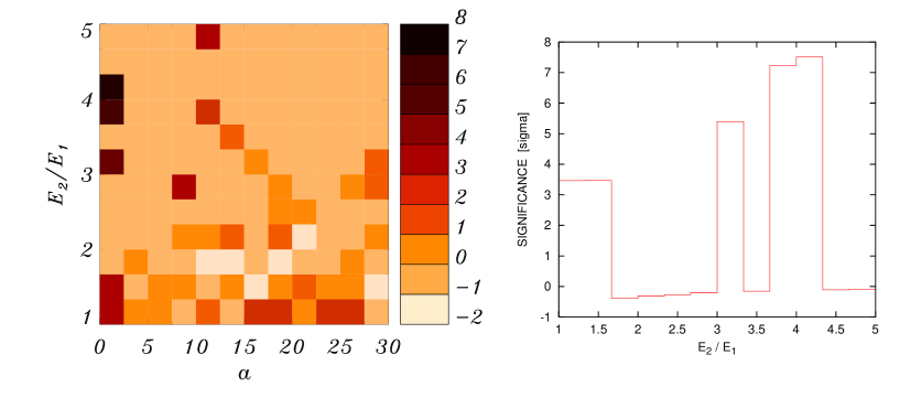
Figure 16: Significance of the correlations in angle and energy ratio in the observed AGASA data. The right panel corresponds to the first angular bin of the left panel ($\alpha<2.5^{\circ}$).

The results are shown in the left panel of Figure 16. A significant excess of pairs is found both at small angles and at similar energies. The right panel shows the one dimensional correlation in $R$ for pairs separated by less than $2.5^{\circ}$, which corresponds to the first angular bin in the left panel. We see here a more than three sigma excess for events with $E_{1}\simeq E_{2}$, which reflects the fact that two doublets and a pair in the triplet have this property. The other quite significant peaks around $R=3$ and 4 reflect the fact that there are doublets with $E_{2}/E_{1}\simeq 4.2,3.7$ and 3.1, something unlikely in a steeply falling spectrum like the one observed and with the present statistics. Magnetic lensing of sources with varied composition is thus a plausible cause of these peaks.

Another feature which can be noticed in the observed multiplets is the fact that all of them have one or two events with energy near or below $50$ EeV, what could be indicative of the presence of a threshold energy associated to the formation of caustics (with the higher energy events in the pairs corresponding to heavier nuclei). This fact also explains the excess observed at similar energies but large angles ($15^{\circ}\div 25^{\circ}$) in the two dimensional correlation (left panel), which seems to be the result of cross correlation between different doublets having similar energies.

- [1] A. A. Ruzmaikin, A. M. Shukurov and D. D. Sokoloff, Kluwer Academic Press, Dordrecht (1988).
- [2] P. P. Kronberg, Rep. Prog. Phys. 57 (1994) 325.
- [3] R. Beck, Galactic and extragalactic magnetic fields, Space Science Reviews 99 (2001) 243.
- [4] J. W. Armstrong, J. M. Cordes and B. J. Rickett, Nature 291(1981) 561.
- [5] M. Giler, J. Wdowczyk and A. W. Wolfendale, J. Phys. G 6 (1980) 1561.
- [6] V. Berezinsky, S. I. Grigori’eva and V. A. Dogiel, Sov. Phys. JETP 69 (1989) 453.
- [7] E. Waxman and J. Miralda-Escudé, Astrophys. J. 472 (1996) L89; J. Miralda-Escudé and E. Waxman, Astrophys. J. 462 (1996) L59.
- [8] T. Stanev, Astrophys. J. 479 (1997) 290.
- [9] G. Medina Tanco, E. De Gouveia dal Pino and J. Horvath, Astrophys. J. 492 (1998) 200.
- [10] G. Sigl, M. Lemoine and P. Biermann, Astropart. Phys. 10 (1999) 141; M. Lemoine, G. Sigl and P. Biermann, astro-ph/9903124.
- [11] D. Harari, S. Mollerach and E. Roulet, JHEP 08 (1999) 022.
- [12] D. Harari, S. Mollerach and E. Roulet, JHEP 02 (2000) 035.
- [13] A. Achterberg et al., astro-ph/9907060.
- [14] See e.g. S. Mollerach and E. Roulet, Gravitational lensing and microlensing, World Scientific, Singapore, (2002).
- [15] Y. Uchihori et al., Astropart. Phys. 13 (2000) 151.
- [16] M. Takeda et al., Astrophys. J 522 (1999) 225.
- [17] M. Takeda et al., Proc. ICRC Hamburg, Germany (2001) 341; M. Teshima, talk at TAUP 2001, Gran Sasso, Italy (2001), in press.
- [18] P. G. Tinyakov and I. I. Tkachev, JETP Lett. 74 (2001) 1.
- [19] J. Alvarez-Muñiz, R. Engel and T. Stanev, astro-ph/0112227.