Xmm–newton observation of Abell 1835 : temperature, mass and gas mass fraction profiles.

We present a study of the medium distant cluster of galaxies Abell 1835 based on Xmm–newton data. The high quality of Xmm–newton data enable us to perform spectro-imaging of the cluster up to large radii. We determine the gas and total mass profiles based on the hydrostatic approach using the $\beta$-model and the temperature profile. For the determination of the temperature profile of the icm, which is needed for the mass determination, we apply a double background subtraction, which accounts for the various kinds of background present (particle and astrophysical background). We find a basically flat temperature profile up to 0.75  $r_{200}$ with a temperature decrease towards the center linked to the cooling flow. We obtain a gas mass fraction of (20.7$\pm 3.7$)%, which is a lower limit on the baryon fraction in this cluster. Using this value as baryon fraction for the entire universe, we obtain by combining our results with results based on primordial nucleosynthesis, an upper limit for $\Omega_{m}<0.5h_{50}^{-1/2}$, which is in good agreement with other recent studies.

1 Introduction

Clusters of galaxies are dark matter dominated and thus are ideal objects to obtain information on this kind of material. A straightforward way to determine the mass profile of a cluster, which consists of roughly 80% dark matter is to use the hydrostatic approach based on the hot x–ray emitting intra-cluster medium (hereafter icm). In order to get reliable results with this approach it is necessary that the examined galaxy cluster is in a relaxed state without ongoing merger activity, which might create shock waves and bias the mass estimate. The validity of the hydrostatic approach for relaxed clusters has been tested via hydrodynamic simulations (Schindler 2001 ; Evrard, Metzler & Navarro 1996). To solve the hydrostatic equation one needs to know the density as well as the temperature distribution of the icm. The latter one requires x–ray observatories, which provide at the same time good spatial as well as spectral resolution. X-ray observatories such as Rosat, Asca, and Beppo-Sax only provided limited combinations of these two requirements and thus the determination of cluster temperature profiles based on these data were subject to large error bars and sometimes different studies on the same object with the same data came to very different conclusions (Irwin & Bregman 2000 ; Markevitch et al. 1998). A subject of hot debate was the question whether there exists a universal declining temperature profile in clusters as suggested by Markevitch et al. (1998) or not. Recently launched x–ray satellites namely Chandra (Weisskopf et al. 2000) and Xmm–newton (Jansen et al. 2001) fullfill now all requirements for an accurate determination of the temperature distribution in clusters up to large radii.

We present here a spectro-imaging study and subsequent mass determination analysis of the medium distant (z=0.25) relaxed galaxy cluster Abell 1835 (Allen et al. 1992) observed during the Xmm–newton Performance Verification phase. Abell 1835 is a relaxed cluster, which hosts a cooling flow in its center (Allen et al. 1996). It belongs to the cooling flow clusters for which no multiphase gas down to low temperatures has been found in the Xmm–newton rgs data (Peterson et al. 2001), and which casts serious doubts on current cooling flow models (Fabian et al. 2001, Molendi & Pizzolato 2001).

We determine the total and gas mass profile of the cluster up to 1.7 Mpc which corresponds to 0.75 virial radius (see section 5). The ratio of gas mass over total mass allows us to determine a lower limit for the baryon fraction of the cluster which can be considered as representative of the mean baryon fraction of the Universe (see White et al. 1993 and references therein). Knowing the baryon density of the Universe based on studies of primordial nucleosynthesis we can give constraints on the cosmological matter density parameter $\Omega_{\mathrm{m}}$.

Our paper is organized as follows : in section 2 we describe the observation. In section 3 we present the data analysis with specific emphasis on vignetting corrections and flare rejection. In section 4, we present first results and a method to correct for different background components : a) particle induced background and b) astrophysical background, which varies across the sky (Snowden et al. 1997). The method is based on a double background subtraction. Section 5 presents our gas and total mass determination and estimate of the baryon fraction of Abell 1835. This is followed in section 6 by the discussion of our results and our conclusions in section 7.

Throughout this article, we use a cosmology with H${}_{0}=50$ km/s/Mpc, $\Omega_{m}=1$ and $\Omega_{\Lambda}=0$ (q${}_{0}=0.5$). One arc-minute corresponds to 297 kpc at the cluster redshift of 0.25.

2 Observation

Xmm–newton observed Abell 1835 in revolution 101 on June 28th 2000. The observation (id 98010101) was taken during the phase of Performance Verification. The total exposure time was 60 ksec. Since we are interested in spatially resolved spectroscopy we concentrate here on data from the epic-instruments (Turner et al. 2001 ; Strüder et al. 2001). During the observation of Abell 1835 the mos1 camera was operating in Large Window mode, which shows a relatively high internal background level, and for which we cannot yet properly account for. Since our work is very sensitive to background uncertainties we discard mos1 data of Abell 1835 in the following and only use data coming from the mos2 and pn camera. For all cameras thin1 filter was used.

3 Data processing

We generate calibrated event files using the tasks emchain and epchain in the xmm sas version 5.0 . For the mos2 data set, we take into account event patterns 0 to 12 and for pn data only single events (pattern=0).

3.1 Flare rejection

The light curve of this observation (see figure 1) is not constant and large variations of intensity are visible. These variations, which we will call “flares” in the following, are caused by soft energy protons produced by solar activity, and which are only visible outside the Earth’s magnetosphere, which corresponds to the orbit of Xmm–newton (see Ehle et al. 2001).

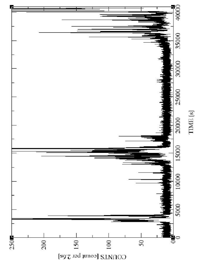
Figure 1: Light curve derived from mos2 camera and event energy between 0.3 and 12 keV.

Unfortunately, the background induced by flares cannot be easily accounted for since it shows spectral variability. Furthermore, the flares reduce the observed signal-to-noise ratio. Therefore it is best to discard flare periods. This reduces the effective exposure time, but improves the signal-to-noise ratio significantly.

Figure 2: Effective exposure time versus count rate threshold for several mos data sets. For the Lockman Hole observations, the revolution 70, respectively 71 was used for mos1, respectively mos2. The count rate threshold was defined as the number of events per 100 s time intervals in the 10 to 12 keV energy band.

Figure 3: Same as figure 2 except it is for pn data sets and that the threshold was defined as the number of events per 100 s time intervals in the 12 to 14 keV energy band.

For our analysis we only consider events inside the field-of-view (fov) and ignore all events outside the fov.

Flares show a hard component observable at high energies easily detectable above 10 keV where the mos cameras are hardly sensitive to X-ray photons. We choose the 10 to 12 keV energy band to monitor the background for the mos2 camera. In order to optimize the background rejection, we analyze the relationship between effective exposure time and the threshold we apply. The results are shown in figure 2 for Abell 1835 and Lockman Hole (revolution 70 and 71) observations. We can see that the behaviour of exposure time versus rejection threshold is similar for all observations, with a flattening at a threshold of about 15 counts/100 s. Thus we can say that this is the optimal threshold for flare rejection, since it limits exposure time loss. A higher threshold does not significantly increase the exposure time and a lower threshold limits severely the remaining effective exposure time. Therefore we adopt in the following analysis a threshold of 15 counts/100 s in the 10 to 12 keV energy band. The same procedure is applied for the pn data (see figure 3). The pn camera provides higher quantum efficiency at high energies than the mos detectors. Because of this we shift our energy window for monitoring the background level to the 12 to 14 keV energy band. Our adopted threshold is 22 counts/100 s.

Of course, the adopted threshold criterion for flare rejection must also be applied to the observations chosen to determine the background.

After applying this flare rejection method, the remaining exposure times are 25750 s for mos2 and 25950 s for pn.

3.2 Vignetting correction

The collecting area of the x–ray telescopes aboard Xmm–newton is not constant across the field of view. The effective area decreases with increasing off-axis angle and is furthermore photon energy dependent. This effect (vignetting) must be taken into account in the case of extended sources, like galaxy clusters, which cover large fractions of the field of view.

To correct for this vignetting effect, we use the method described by Arnaud et al. (2001a). Briefly, this method consists of calculating a weight parameter for each event. According to event energy, this parameter is defined as the ratio of on–axis effective area to effective area at the event position on the detector. Thus, all weight parameters are greater or equal to unity.

4 Data analysis

4.1 Morphology

Figure 4: Mos2+pn vignetting corrected image of Abell 1835 in sky coordinates in the 0.3 to 3 keV energy band. This image is filtered with a $\sigma$=2.2′ Gaussian. The contours come from an 0.3 to 3 keV only mos2 image where the gaps between ccds cannot change the shape of these contours. The contour levels are 0.25, 1, 2, 4, 8, 16 and 28 photons by 1.1″ $\times$1.1″ pixel.

As can be seen in figure 4, Abell 1835 is a compact cluster. There is no strong evidence of substructures which suggests that the cluster is in a relaxed state. The intensity is very peaked in the center due to the presence of a cooling flow (Allen et al. 1996; Schmidt, Allen & Fabian 2001; Peterson et al. 2001).

4.2 Spectra

Since we apply the described vignetting correction method, we can use the on–axis response (i.e. effective area $\times$ redistribution matrix) files : m2_thin1v9q20t5r6_all_15.rsp for the mos2 camera and epn_ff20_sY9_thin.rsp for the pn. There exist different response matrix files for the pn-chips, which correspond to the different nodes. We use Y9, which is the node farthest away from the readout, with lowest resolution. We tested the different response files of the different nodes and could not find any detectable difference when performing spectral fits. Due to the remaining uncertainties of the response files at very low energy, we exclude events with energy below 0.3 keV for all spectral fits.

4.2.1 Background treatment

Due to the fact that clusters of galaxies are extended and generally low surface brightness sources, the correct determination of the background is important for data fitting and modelling. Since cluster emission decreases with radius from the center, the background component becomes more and more important with increasing radius.

After removing the flare component by excising high background intensity time intervals, two other background components remain :

• high energy particles like cosmic–rays pass through the satellite and deposit a fraction of their energy on the detector. They are not affected by the telescope vignetting. These particles induce instrumental fluorescent lines coming from material aboard the satellite. This kind of background is well monitored by blank–sky observations based on several high galactic latitude observations in which x–ray sources were excised. These observations were compiled by D. Lumb (2002) for each epic camera ;

• the astrophysical x–ray background. The soft component of this background is position dependent and changes across the sky. Therefore it is not necessarily well monitored by blank-field observations taken at different positions on the sky.

A description of the following method to correct for each background component can also be found in Majerowicz & Neumann (2001) and Pratt et al. (2001). A similar method was used by Markevitch & Vikhlinin (2001) for Chandra data.

In the data sets of Abell 1835 and of the blank-sky observations, which we use for background subtraction, we attribute to each event a weighting factor to correct for vignetting (see section 3.2). This is obviously wrong in case of particle events, which are not vignetted. If the particle background (after flare rejection, see section 3.1) is constant with time in terms of spectrum shape, what we assume here, we can correct for the falsely attributed weighting factor by subtracting the background spectrum in the same detector region as the source spectrum. In order to account for possible long time intensity variations in the particle induced background, we determine the count rates of source and background observation at high energies ($>10$ keV), where the quantum efficiency for X-ray photons are low. The ratio of the countrates is used to normalize the corresponding background in the spectral fits. For the mos2 we use the 10-12 keV band for determining the background intensity, and for the pn-data the 12-14 keV band, respectively. In our case, a normalization factor of 1 is found. With this method we correct for the particle background. However we do not yet necessarily account for the spatial variations of the cxb.

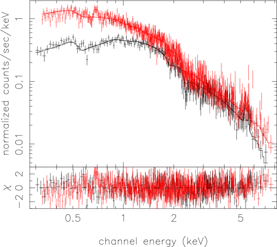
Figure 5: A mos2 (lower) and pn (upper) combined fit of fully background corrected spectra in the outside region of the cooling flow (see section 4.4).

Abell 1835 is located in a peculiar region of the sky, where an excess of low energy cxb can be seen (Snowden et al. 1997). To correct for this local excess of the cxb, we use regions of the detector in which x–ray emission from the cluster is negligible. We assume in the following that the cxb does not change significantly across the 30′ of detector field of view. We extract a spectrum in the annulus between 7′ and 12′ from the cluster center. From this spectrum outside of the cluster, we subtract the blank-sky spectrum extracted from the same detector region. The residual spectrum represents the difference of the cxb between the observation of Abell 1835 and the blank-sky observations. These residuals were subsequently subtracted from the cluster spectrum, from which we already subtracted the blank-sky spectrum in the same detector regions. We thus yield spectra which are now properly corrected for the two background components described above. In figure 5, we present background corrected spectra from mos2 and pn data which will be used in section 4.4 for the estimate of the mean temperature outside the cooling flow region.

For the pn data there exists another source of contamination, the so called out of time (oot) events, i.e. events counted during the read-out (see Strüder et al. 2001). They are visible as a jet–like structure in figure 4. To estimate the impact of these oot events on the temperature determination, we extract spectra in regions defined in table 1 in which we exclude the oot affected regions. Comparing the fit results of those oot corrected spectra with the non-corrected oot spectra we find a slight increase in the temperature estimates of a few percent, however, always well within the error bars. We thus conclude that the oot’s do not play an important role in the temperature determination for this particular observation. In the following analysis of pn data, we use the non-oot corrected spectra.

4.2.2 Temperature profile

Annulus (’)		T (keV) ($\chi^{2}_{\mathrm{red}}$/$dof$)			A (solar)
$r_{1}$	$r_{2}$	mos2	pn	mos2+pn	mos2+pn
0.0	0.25	$4.81\pm 0.25$ (1.17/307)	$4.43\pm 0.12$ (1.17/706)	$4.52\pm 0.10$ (1.18/1014)	$0.42\pm 0.05$
0.25	0.75	$6.67\pm 0.29$ (0.98/371)	$6.16\pm 0.20$ (1.12/933)	$6.31\pm 0.16$ (1.09/1305)	$0.30\pm 0.04$
0.75	1.5	$7.29^{+0.45}_{-0.39}$ (0.95/325)	$6.76\pm 0.27$ (1.02/749)	$6.94\pm 0.22$ (1.00/1075)	$0.23\pm 0.05$
1.5	2.25	$7.24^{+0.87}_{-0.63}$ (0.91/229)	$7.15^{+0.50}_{-0.46}$ (1.02/509)	$7.19\pm 0.38$ (0.99/739)	$0.32\pm 0.08$
2.25	3.33	$6.87^{+1.15}_{-0.95}$ (1.10/164)	$8.31^{+1.13}_{-1.05}$ (0.90/339)	$7.68^{+0.89}_{-0.73}$ (0.97/504)	$0.27\pm 0.13$
3.33	6.0	$6.98^{+3.35}_{-1.89}$ (0.95/53)	$7.80^{+3.90}_{-2.09}$ (1.15/84)	$7.31^{+2.32}_{-1.33}$ (1.06/138)	$<0.9$

Table 1: Results for the isothermal model fits derived from equ. (1) where the free parameters are the temperature T and the abundance A. The galactic hydrogen column density value n_H is frozen to the galactic value of 2.24$\times$10²⁰ cm^-2 (Dickey & Lockman 1990). The spectra are extracted in annuli with inner radius $r_{1}$ and outer radius $r_{2}$. The errors have a confidence level of 90%.

Abell 1835 appears to be a relaxed cluster of galaxies (see section 4.1). Therefore we assume that the temperature structure of this cluster is spherically symmetric. We extract cluster spectra in concentric annuli around the cluster center. The size we choose for the annuli is a compromise between number of source counts to have sufficient statistics on one hand and small enough regions to determine the temperature profile with small bins on the other hand. In our analysis, we exclude the most luminous point sources which are located inside the field of view of the cameras.

We group spectra such that each bin has a signal-to-noise ratio greater than 3$\sigma$ after background subtraction. This grouping allows us to assume Gauss statistics, which is important for $\chi^{2}$ fitting.

For the fit to the spectra, we use xspec version 11.0.1 (Arnaud 1996) and we model the obtained spectra with :

$$\mathrm{Model}=\mathrm{Wabs(\mbox{n${}_{\mathrm{H}}$})}\times\mathrm{Mekal(T,A)}$$ (1)

where $\mathrm{Wabs}$ is a photo electric absorption model (Morrisson & McCammon 1983) and $\mathrm{Mekal}$ a single temperature plasma emission model (Mewe et al. 1985 ; Kaastra 1992 ; Liedahl et al. 1995). The free parameters are the galactic hydrogen column density value n_H, the x–ray temperature kT and the metallicity (abundance) A.

First we fit all the spectra with a fixed galactic absorption n${}_{\mathrm{H}}=2.24\times$10²⁰ cm^-2 given by Dickey & Lockman (1990) from 21 cm line measurements. Results are shown in table 1. In a second spectral analysis we leave the n_H value as a free fit parameter (see table 2). The resulting fit temperatures agree very well with those obtained with fixed n_H which gives us high confidence in our spectral analysis and our background subtraction. Figure 8 shows the fit results for n_H which are in good agreement with the measurements from the 21 cm line. Figure 6 shows the resulting temperature profile up to a physical radius of 1.8 Mpc derived from the table 1. Figure 7 shows the metal abundance profile up to 1 Mpc.

Figure 6: Abell 1835 temperature profile (see table 1) derived from a combined fit of the mos2 and pn cameras where the n_H value is equal to the galactic value at the sky position of Abell 1835. The mean temperature (see section 4.4) is represented by the dashed line.

Figure 7: Abundance profile (see table 1) and its mean value outside the cooling flow (dashed line, see section 4.4) in units of solar metallicity up to 1 Mpc.

Figure 8: Absorption column density n_H profile from table 2. The dashed line represents the galactic value of 2.24$\times$10²⁰ cm^-2 (Dickey & Lockman 1990).

Annulus	T (keV)	nH (1020 cm2)	$\chi^{2}_{\mathrm{red}}$/$dof$
1	$4.60^{+0.23}_{-0.12}$	$1.90\pm 0.30$	1.17/1013
2	$6.61\pm 0.20$	$1.64\pm 0.23$	1.07/1304
3	$7.31^{+0.33}_{-0.29}$	$1.56\pm 0.32$	0.99/1074
4	$7.34^{+0.66}_{-0.47}$	$1.95\pm 0.52$	0.99/738
5	$7.58^{+1.13}_{-0.96}$	$2.16^{+0.90}_{-0.78}$	0.97/503
6	$7.28^{+3.30}_{-1.70}$	$2.30^{+2.38}_{-1.50}$	1.07/137

Table 2: Spectral fit results with n_H value as free fit parameter (mos2+pn combined fits).

4.3 Psf corrected temperature profile

Abell 1835 is a medium distant galaxy cluster with a very peaked surface brightness profile (see figure 11) due to the presence of a cooling flow in the centre. Because of this, the point spread function (psf) of Xmm–newton (Griffiths et al. 2002, Ghizzardi 2001) potentially blurs the central regions of the cluster, which might influence the observed temperature profile (see also Markevitch 2002). In order to assess this influence we perform another spectral analysis, in which we take into account the psf of Xmm–newton. We apply the method which is extensively described by Pratt & Arnaud (2002).

For our analysis we assume that the psf is constant across the extent of the cluster and that its shape is energy independent. We calculate the flux redistribution of all temperature bins due to blurring. This computation is based on a convolution of a double $\beta$-model, which is fitted to the surface brightness profile and which gave the following parameters (this fit was performed taking the psf into account). Subsequently, based on these model parameters ($\beta_{\mathrm{in}}=0.49$, $r_{c,\mathrm{in}}=0.1$’, $\beta_{\mathrm{out}}=0.74$, $r_{c,\mathrm{out}}=0.79$’) we calculate the flux contribution of bin $i$ to bin $j$. The result can thus be interpreted as a matrix. The corresponding redistribution elements are shown in figure 9 for the pn data. The redistribution for mos2 is similar. As an illustration of the importance of the psf effect in the centre : only 65% of the flux of the second bin ($i=2$) are actually observed in the second bin ($j=2$). The remaining 35% are distributed in other bins ($i=2,j\neq 2$).

After the determination of the redistibution or matrix elements we fit simultaneously the different spectra of our six temperature bins. We take into account the different flux contributions of each bin by fixing the ratios of normalization of the fitted spectral models based on our calculated redistribution matrix. Our resulting $\chi^{2}_{\mathrm{red}}$ for the combined fit is $\chi^{2}_{\mathrm{red}}=1.05$ for 4775 degrees of freedom. The resulting temperature profile is displayed in figure 10 as well as in table 3. Briefly, when we take into account the psf we obtain a steeper temperature gradient in the cooling flow region of the cluster. The temperature estimates at larger radii are hardly affected by the psf and are within the error bars of the non-psf corrected analysis. Our study presented here is focussed on the external regions of the cluster, therefore we conclude that the psf does not have an important impact on our analysis (see below).

Figure 9: Redistribution of the cluster flux for the pn camera in the radial bins we use to derive the temperature profile. The triangles represents the flux coming from the bin, the squares from all inner bins to the bin, the losanges from all outer bins to the bin and the crosses from the central bin to the bin.

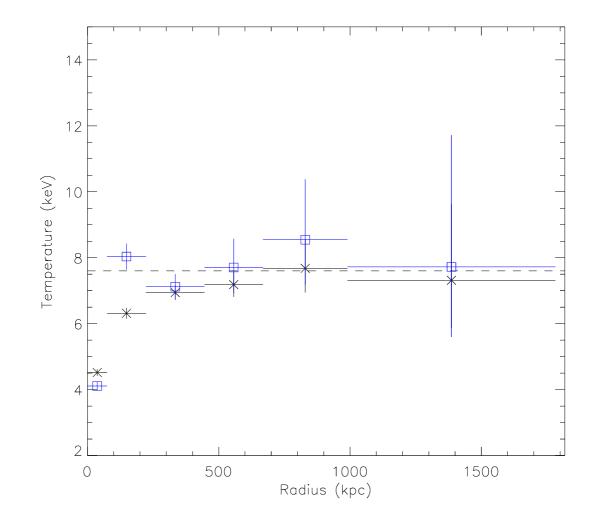
Figure 10: Temperature profile of Abell 1835 corrected for the PSF (from table 3, squares) comparing to the previous one (from table 1, crosses). The dashed line represents the mean temperature outside the cooling flow region (see section 4.4).

Annulus	T (keV)	Abundance (solar)
1	$4.11\pm 0.12$	$0.43\pm 0.05$
2	$8.03\pm 0.39$	$0.32^{+0.06}_{-0.08}$
3	$7.12\pm 0.36$	$0.19\pm 0.08$
4	$7.70^{+0.87}_{-0.77}$	$0.37^{+0.16}_{-0.14}$
5	$8.55^{+1.36}_{-1.84}$	$<0.5$
6	$7.72^{+3.99}_{-2.12}$	$<1.0$

Table 3: Temperature estimate in each annulus for psf corrected mos2+pn combined fit.

In the following analysis, we will exclusively use the psf corrected temperature profile.

4.4 Mean temperature outside the cooling flow

We use the background subtracted spectra for mos2 and pn data in an annulus between 1′ and 6′ — between 300 and 1800 kpc — around the cluster center to obtain the mean temperature of the cluster outside the cooling flow region. We perform a combined fit using the model described above in equ. (1) with a n_H value fixed to 2.24$\times$10²⁰ cm^-2. We find a temperature of $7.6\pm 0.4$ keV and an abundance of 0.25$\pm 0.05$ with 90% confidence level.

4.5 Surface brightness profile

We extract surface brightness profiles from the cluster data. In order to account for vignetting effects we use again the photon weighting method described in section 3.2. In our specific case using the weight factor for each event to account for vignetting, the count rate $CR_{i}$ in the i-th annulus is defined as :

$$CR_{i}={{1}\over{T_{\mathrm{expo}}}}{{\sum_{j=1}^{n}w_{j}}\over{A_{i}}}$$ (2)

where $n$ is the number of events in the i-th annulus, $w_{j}$ the event weight parameter, $A_{i}$ the surface of the selected annulus and $T_{\mathrm{expo}}$ the exposure time. In this case, the Poisson error becomes :

$$\sigma_{i}={{1}\over{T_{\mathrm{expo}}}}{{\sqrt{\sum_{j=1}^{n}w_{j}^{2}}}\over{A_{i}}}$$ (3)

Serendipitous sources in the field of view are excluded. Figure 11 shows the surface brightness profile of Abell 1835 derived from the mos2 and pn cameras in the 0.3 to 3 keV energy band.

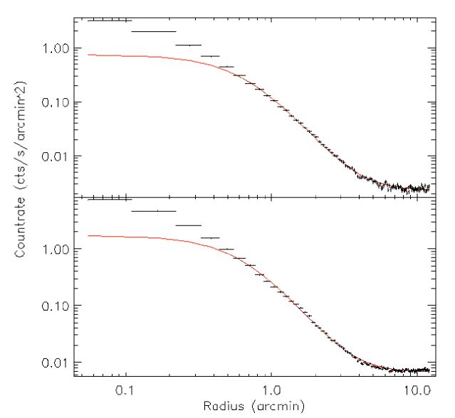
Figure 11: Abell 1835 surface brightness profiles from mos2 (upper panel) and from pn (lower panel) in 0.3 to 3 keV energy band (1′corresponds to 297 kpc). The error bars are one $\sigma$ based on Poisson statistics. The resulting $\beta$-model fits are shown in full line.

The surface brightness profile is fitted with a $\beta$-model (Cavaliere & Fusco–Femiano 1976) in which the surface brightness $S$ is defined as :

$$S(r)=S_{0}{\Bigg{(}1+{\bigg{(}{{r}\over{r_{c}}}\bigg{)}}^{2}\Bigg{)}}^{-3\beta+{{1}\over{2}}}+B$$ (4)

where $S_{0}$ is the central intensity, $r_{c}$ the core radius, $\beta$ the slope parameter and $B$ the background intensity. All these parameters must be fitted.

Abell 1835 hosts a cooling flow in its center (see above). Figure 11 shows the characteristic peak of intensity for cooling flows towards the center (e.g. Fabian 1994). In order to avoid fitting in the cooling flow region we choose to exclude a region with a radius of roughly 0.1 r₂₀₀ (see equ. (5)) — i.e. 0.7′— around the center for the $\beta$-model fit. Indeed Neumann & Arnaud (1999) showed that below 0.1 r₂₀₀ the surface brightness profiles for nearby clusters show a large dispersion due to cooling flow but they look remarkably similar above 0.1 r₂₀₀. The best fit parameters are $\beta=0.704\pm 0.005$ and a core radius $r_{c}=202.3\pm 7.1$ kpc (i.e. $r_{c}=0.681\pm 0.024$′) for the mos2-data. The uncertainties are 68% confidence level. We also perform a $\beta$-model fit with the surface brightness profile extracted from the pn data for consistency. We find in this second case $\beta=0.708^{+0.012}_{-0.007}$, $r_{c}=196.9^{+5.1}_{-5.3}$ kpc (i.e. $r_{c}=0.663^{+0.017}_{-0.018}$ ′). These fit parameters are thus in good agreement with those found with the mos2 camera.

Our found parameters of $\beta$ and $r_{c}$ are in relatively good agreement with the results found by Neumann & Arnaud (1999) for nearby clusters.

5 Mass analysis

We assume in the following that the cluster is virialized up to $r_{200}$, the radius in which the mean density of the cluster is 200 times the critical mass density. For the calculation of $r_{200}=r_{\rm{virial}}$ we use the relation by Evrard et al. (1996) :

$$r_{200}=3690\sqrt{{{T}\over{10\,\mathrm{keV}}}}{(1+z)}^{-{{3}\over{2}}}$$ (5)

Using the mean temperature of 7.6 keV (see section 4.4), we find $r_{200}=2293$ kpc.

5.1 Intra cluster medium mass

Assuming that the radial icm distribution follows a $\beta$-model, the electron density $n_{e}$ can be written :

$$n_{e}(r)=n_{e0}{\Bigg{(}1+{\bigg{(}{{r}\over{r_{c}}}\bigg{)}}^{2}\Bigg{)}}^{-{{3}\over{2}}\beta}$$ (6)

From the electron density we calculate the total gas density of the icm and determine the icm mass by integrating equ. (6). We obtain a central electron density $n_{e0}=1.47\pm 0.02\times 10^{-2}$ cm^-3 (68% confidence level) assuming a temperature of 7.6 keV and using the $\beta$-model parameters determined in section 4.5. Temperature variations in the uncertainties do not change our values for the electron density. The error bars of $n_{e0}$ are calculated from the errors of the $\beta$-model parameters. We verify that the cluster temperature has no effect on the estimate of $n_{e0}$ with the selected energy range.

Figure 12: Abell 1835 gas mass profile. The error bars (dotted line) are a confidence level of 68%. The gas mass profile (full line) is derived from the best fit parameters.

The icm mass profile is shown in figure 12. We find M${}_{\mathrm{gas}}=2.56\pm 0.08\times 10^{14}$ M_⊙ within $r=1.7$ Mpc or 0.75 $r_{200}$ with a confidence level of 68%.

We want to stress that we underestimate the central gas density in the centre due to neglecting the cooling flow excess. However, this underestimation at small radii does not play a significant role when we integrate the gas mass out to large radii.

In fact, when we fit the surface brightness profile (figure 11) so that we only account for the inner 210 kpc, we find $\beta$=0.49, $r_{c}$=52 kpc and $n_{e0}=5.55\times 10^{-2}$ cm^-3. By integrating equ. (6) with these parameters, we find a gas mass at r=0.1 $r_{200}$, which is 18% higher than the one using the global $\beta$-model fit parameters. At $r=0.75r_{200}$, which is the radius up to which we can constrain the temperature and thus total mass profile we underestimate the gas mass by 1% due to neglecting the gas mass linked to the central gas excess with respect to our global $\beta$-model , which is negligible.

5.2 Cluster total mass

Assuming spherical symmetry and hydrostatic equilibrium, we calculate the gravitational mass of the cluster Abell 1835 with the hydrostatic equation :

$$\mathrm{M}_{\mathrm{tot}}(<r)=-{{k\mathrm{T}}\over{G\mu m_{p}}}r\Bigg{(}{{d\ln n_{e}}\over{d\ln r}}+{{d\ln\mathrm{T}}\over{d\ln r}}\Bigg{)}$$ (7)

where $k$ is the Boltzmann constant, T the gas temperature, $G$ the gravitational constant, $\mu$ the mean molecular weight of the gas ($\mu\sim 0.6$), $m_{p}$ the proton mass and $n_{e}$ the electronic density. Including equ. (6) in equ. (7), M can be written :

$$\mathrm{M}_{\mathrm{tot}}(<r)=-{{k}\over{G\mu m_{p}}}r^{2}\Bigg{(}{{d\mathrm{T}}\over{dr}}-3\beta\mathrm{T}{{r}\over{r^{2}+r_{c}^{2}}}\Bigg{)}$$ (8)

Figure 13: Abell 1835 total mass profile using the psf corrected temperature profile (see section 4.3). Error bars are at 68% confidence level(same display convention as figure 12).

In order to account for the error bars in the temperature profile, we use a Monte–Carlo method described by Neumann & Böhringer (1995). This method allows to transform error bars of the temperature profile into error bars of the mass profile. This transformation is done by calculating randomly temperature profiles, which fit in the actual measured temperature profile and to subsequently calculate the mass profile corresponding to the randomly determined temperature profile. We determine 10000 random temperature profiles. From the corresponding 10000 mass profiles we calculate the mean mass profile and the errors. The uncertainties are determined by taking into account the uncertainties of the temperature profile (90% confidence level) and the standard deviation of the mass at a given radius. The resulting errors are calculated so that they correspond to 1$\sigma$ error bars (68% confidence level). The mass profile is shown in Fig.13. At a radius corresponding to 75% of the virial radius (or 1.7 Mpc) we obtain a total mass of : $M_{tot}=1.23\pm 0.18\times 10^{15}$ M_⊙ (68% confidence level).

Assuming that Abell 1835 is isothermal with a temperature of 7.6 keV (see section 4.4), equ. (8) can be written as :

$$\mathrm{M}_{\mathrm{tot}}(<r)={{3k\beta}\over{G\mu m_{p}}}\mathrm{T}{{r^{3}}\over{r^{2}+r_{c}^{2}}}$$ (9)

In this case taking into account error bars on T, $\beta$ and $r_{c}$ parameters, the total mass of Abell 1835 is $1.00\pm 0.06\times 10^{15}$ M_⊙ which is consistent with the mass obtained using the Monte-Carlo approach. This was expected since the temperature profile of Abell 1835 (see figure 10) seems to be isothermal at high radii.

5.3 Gas mass fraction

Figure 14: Abell 1835 gas mass fraction profile. Error bars are at 68% confidence level (same display convention as figure 12).

The gas mass fraction is simply the ratio of the icm mass to the total mass. The profile of the gas mass fraction of Abell 1835 is shown in figure 14. We do not display the gas mass fraction below 10% of the virial radius because of the cooling flow region and our underestimate of the gas mass there (see section 4.5). The errors bar are calculated with classical error propagation and are at a confidence level of 68%. Within $r=0.75\,r_{200}$, we find $f_{gas}h_{50}^{-1.5}=0.207\pm 0.037$ where $h_{50}$ is the present time Hubble constant in units of 50 km/s/Mpc.

6 Discussion

6.1 The gas mass fraction and implications for cosmology

Abell 1835 is an ideal cluster to determine the gas mass profile with the hydrostatic approach, since the Xmm–newton image does not show indications of substructure at large scales, which might contaminate the mass determination.

Our determined gas mass fraction profile of Abell 1835, which we determine up to 0.75 $r_{200}$ is essentially flat. The mean value is about 21% and within 0.75 $r_{200}$ we obtain a gas mass fraction of $0.207\pm 0.037h_{50}^{-3/2}$. We can take this gas mass fraction as lower limit for the baryon fraction in the cluster because we do not take into account other contributions of baryons, such as stars or interstellar medium. Extrapolating this lower limit through out the universe (which was shown to be valid by White et al. (1993) and references therein), we can determine the cosmological matter density parameter $\Omega_{m}$ by combining our result with studies based on primordial nucleosynthesis, which give firm constraints on the density parameter of baryons in the universe. Recent results give $\Omega_{b}h_{50}^{2}=0.080\pm 0.008$ (Burles et al. 2001). We can thus apply :

$${{M_{\mathrm{gas}}}\over{M_{\mathrm{tot}}}}=0.207\pm 0.037h_{50}^{-3/2}={{\Omega_{\mathrm{b}}}\over{\Omega_{\mathrm{m}}}}={{0.08\pm 0.008h_{50}^{-2}}\over{\Omega_{\mathrm{m}}}}$$ (10)

If the icm was the only source of baryons in clusters, above equation gives us $\Omega_{\mathrm{m}}=0.386\pm 0.108$ (68% confidence level). However, since there exist other baryon sources in Abell 1835 such as galaxies, this implies that our result is an upper limit with : $\Omega_{\mathrm{m}}<0.5h_{50}^{-1/2}$. This result is in very good agreement with other recent results based on cmb measurements combined with redshift surveys (Efstathiou et al. 2001) and studies on distant supernovæ (Perlmutter et al. 1999) which favor a low density universe with a cosmological constant. If we additionally knew the baryon fraction in galaxies up to high precision, we could put even tighter constraints on $\Omega_{m}$.

6.2 The temperature profile – comparison with other recent studies

A lot of effort has been spent already for the determination of temperature profiles in the icm. The corresponding results vary from each study to another quite significantly. There have been reported declining temperature profiles, with a more or less universal shape based on Asca and Beppo-sax data (Markevitch et al. 1998, de Grandi & Molendi 2001). Other studies based on data from the same instruments, on the contrary, find flat temperature profiles or profiles with large dispersions (Irwin & Bregman 2000, White et al 2000).

All these studies are limited to radii smaller than 0.5 $r_{200}$ due to instrumental limitations. Furthermore, studies based on Asca and Beppo-sax were subject to possible systematic uncertainties due to the large point spread function of the mirrors, which additionally can vary in size depending on energy. Chandra results presented by Allen, Schmidt & Fabian (2001) suggest that massive, relaxed clusters are isothermal up to $r_{2500}$ and show a universal temperature decline in the center linked to the cooling flow.

Xmm–newton with its better spatial resolution than Asca and Beppo-sax and larger effective area than comparable observatories allows to a) better constrain the temperature profiles and b) to trace them out to larger radii. So far studies based on Xmm–newton show either flat profiles (Arnaud et al. 2001a ; Tamura et al. 2001) for hot clusters, which is in agreement with the results by Allen et al. (2001) on Chandra data of clusters. A Xmm–newton study on the cool cluster Sérsic 159-03, however, shows a dramatic temperature decline in the outer parts of the cluster (Kaastra et al. 2001).

Figure 15: Abell 1835 temperature profile and the comparison with the universal profile derived by Allen et al. (2001) and extrapolated to 0.75 $r_{200}$ (dotted line)

Our results suggest strongly a flat temperature profile with a decline towards the center linked to the cooling flow present in Abell 1835 (Peterson et al. 2001, Schmidt et al. 2001 and references therein). This profile fits well with the empirically found model by Allen et al. (2001), which is valid up to $r_{2500}$, which corresponds roughly to $0.3\times r_{200}$ and which is displayed in Fig 15. However, an individual study undertaken by Schmidt et al. (2001) on Abell 1835 observed with Chandra shows a temperature profile which is increasing with radius. At radii larger than 400 kpc Schmidt et al. (2001) find temperature estimates of about 12 keV, which is inconsistent with our Xmm–newton results. The fact that we find good agreement between the individual spectral modeling of mos2 and pn cameras gives us confidence in our results.

While undertaking our study concerning the background subtraction we observed that minor differences in the extraction of flares between background and source observation can lead to declining or increasing temperature profiles. Doing monitoring on the background level we find that quiescent periods do not always have the same background level and have sometimes, even though rarely, intensities close or above the threshold criterion to extract flares. In order to screen the data properly for background variations and to determine the level of the particle (instrumental) background accurately it is important to look at parts of the observation where no astrophysical source emission can be detected like the high energy part of the spectrum, where only particle background can be seen (the particle background has a hard spectrum and the effective area of Xmm–newton at energies above 10 keV for x–ray photons is relatively small). It is important to compare and to apply exactly the same flare rejection for both the source and the background observation to avoid wrong background subtraction, which can bias the temperature estimates. Observing a temperature profile which increases with radius can be an indication of a slightly higher particle background in the source observation than in the background observation.

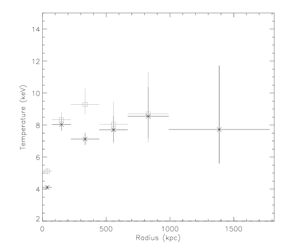
Figure 16: Temperature profile of Abell 1835 corrected for the PSF (from table 3, crosses) comparing to the Chandra one (squares) obtained by Markevitch (2002).

The presence of remaining solar flares in the analysis of Schmidt et al. (2001) was recently discussed by Markevitch (2002), who reanalyzed the Chandra data of Abell 1835. Markevitch (2002) found that a temperature profile analysis based on a more thorough flare treatment leads to a basically flat temperature profile in the outer parts of the cluster, which agrees well with our derived temperature profile (see figure 16) at large scales.

6.3 Global temperature estimates

There is some dispersion observable between past temperature determinations of Abell 1835 based on Asca-data. Allen & Fabian (1998) found a temperature of $9.8^{+2.3}_{-1.3}$ keV, based on Asca-sis and gis-data, including a multiphase cooling flow model, which is now known not to be an accurate description for the cooling flow of Abell 1835 (Peterson et al. 2001). White (2000) only used Asca-gis data and obtained an overall temperature of kT=$8.5^{+1.5}_{-0.5}$ keV when applying a multiphase cooling flow model and kT=$8.2\pm 0.5$ keV when using a single temperature model. Both results are consistent within the error bars with our results of kT=7.6$\pm 0.4$ keV. Furthermore, Mushotzky & Scharf (1997) found a temperature estimate of kT=$8.2\pm 0.5$ keV, which is again comparable with our results and the ones of White (2000). The results of Allen & Fabian (1998) agree within the error bars with other results based on Asca, but are higher than our mean temperature. While our temperature results are somewhat lower than the results of Asca, the Chandra results for the temperature of Abell 1835 by Schmidt et al. (2001) are above the results based on Asca.

7 Conclusion

Xmm–newton data allow us to measure the temperature profile of Abell 1835 up to 0.75 $r_{200}$. In order to determine the temperature profile of the cluster accurately we apply a method, which corrects for the various kinds of background and a photon weighting method which allows to correct for vignetting effects. We correct the temperature profile for psf-effects and see that the resulting profile is not affected by the psf at large radii.

Our resulting psf corrected temperature profile is consistent with being flat in the outer parts. The mean cluster temperature is 7.6 keV outside the cooling flow region. In the central parts, below a radius of 1′(300 kpc) we see a temperature decline linked to the cooling flow of the cluster. We fit a $\beta$-model to the outer radii of the surface brightness profile of Abell 1835 and obtain the best fit results of $\beta=0.704\pm 0.005$ and $r_{c}=202.3\pm 7.1$ kpc. We use these best fit parameters as input for the hydrostatic approach to calculate the mass profile of the cluster and find a mass at 0.75 $r_{200}$ of $1.23\pm 0.18\times 10^{15}$ M_⊙. The corresponding gas mass fraction, which is constant with radius at radii $r>0.1\,r_{200}$, is with 20.7%$\pm 3.7$ comparable with the results found in other studies.

Our global temperature estimate for Abell 1835 based on Xmm–newton is somewhat low when compared to other results, but agree in the error bars with other studies based on Asca-data. We assume that these discrepencies are linked to small remaining uncertainties in the calibration of Xmm–newton , and on which is still being worked on.

- (1) Allen S.W., Edge A.C., Fabian A.C., Böhringer H., Crawford C.S., Ebeling H., Johnstone R.M., Naylor T., Schwarz R.A., 1992, MNRAS, 259, 67
- (2) Allen S.W., Edge A.C., Bautz M.W., Furuzawa A., Tawara Y., 1996, MNRAS, 293, 263
- (3) Allen S.W. & Fabian A.C., 1998, MNRAS, 297, L57
- (4) Allen S.W., Schmidt R.W. & Fabian A.C., 2001, submitted to MNRAS, preprint astro-ph/0110610
- (5) Arnaud K.A., 1996, Astronomical Data Analysis Software and Systems V, eds. Jacoby G. and Barnes J., p17, ASP Conf. Series volume 101
- (6) Arnaud M. & Evrard A.E., 1999, MNRAS, 305, 631
- (7) Arnaud M., Neumann D.M., Aghanim N., Gastaud R., Majerowicz S., Hughes J.P., 2001a A&A, 365, L80
- (8) Burles S., Nollett K.M., Turner M.S., 2001, ApJL in press, preprint astro-ph/0010171
- (9) Cavaliere A., Fusco–Femiano R., 1976, A&A, 49, 137
- (10) De Grandi S. & Molendi S., 2001, submitted to ApJ, preprint astro-ph/0110469
- (11) Dickey J.M., Lockman F.J., 1990, ARAA, 28, 215
- (12) Efstathiou G., Moody S., Peacock J.A., et al., 2001, submitted to MNRAS, preprint astro-ph/0109152
- (13) Ehle M., Breitfellner M., Dahlem M., Guainazzi M., Rodriguez P., Santos–Lleo M., Schartel N., Tomas L., 2001, Xmm–newton User’s Handbook, Issue 2.0
- (14) Evrard A.E., Metzler C.A., Navarro J.F., 1996, ApJ, 469, 494
- (15) Fabian A.C., 1994, ARAA, 32, 277
- (16) Fabian A.C., Mushotzky R.F., Nulsen P.E.J., Peterson J.R., 2001, MNRAS, 321, L20
- (17) Ghizzardi S., 2001, epic-mct-tn-011 (xmm-soc-cal-tn-0022)
- (18) Griffiths G., 2002, in preparation
- (19) Irwin J.A. & Bregman J.N., 2000, ApJ, 538, 543
- (20) Jansen F., Lumb D., Altieri B., et al., 2001, A&A, 365, L1
- (21) Kaastra J.S., An x-ray spectral Code for Optically Thin Plasma, Internal Sron–Leiden Report, updated version 2.0
- (22) Kaastra J.S., Ferrigno C., Tamura T., Paerels F.B.S., Peterson J.R., Mittaz J.P.D., 2001, A&A, 365, L99
- (23) Liedahl D.A., Osterheld A.L., Goldstein W.H., 1995, ApJL, 438, 115
- (24) Lumb D., 2002, XMM-SOC-CAL-TN-0016
- (25) Majerowicz S., Neumann D.M., 2001, Galaxy Clusters and the High–Redshift Universe, eds. D.M. Neumann and J. Trân Thanh Van
- (26) Markevitch M., Forman W.R., Sarazin C.L., Vikhlinin A., 1998, ApJ, 503, 77
- (27) Markevitch M. & Vikhlinin A., 2001, ApJ in press, preprint astro-ph/0105093
- (28) Markevitch M., astro-ph/0205333
- (29) Mewe R., Gronenschild E.H.B.M., van den Oord G.H.J., 1985, A&AS, 65, 511
- (30) Molendi S. & Pizzolato F., 2001, ApJ, 560, 194
- (31) Morrisson R. & McCammon D., 1983, ApJ, 270, 119
- (32) Mushotzky R.F., & Scharf C.A., 1997, ApJ, 482, L13
- (33) Neumann D.M., Böhringer H., A&A, 301, 865
- (34) Neumann D.M., Arnaud M., 1999, A&A, 348, 711
- (35) Perlmutter S., Aldering G., Goldhaber G., et al., 1999, ApJ, 517, 565
- (36) Peterson J.R., Paerels F.B.S., Kaastra J.S., Arnaud M., Reiprich T.H., Fabian A.C., Mushotzky R.F., Jernigan J.G., Sakelliou I., 2001, A&A, 365, L104
- (37) Pratt G.W., Arnaud M., Aghanim N., 2001, Galaxy Clusters and the High–Redshift Universe, eds. D.M. Neumann and J. Trân Thanh Van, astro-ph/0105431
- (38) Pratt G.W., Arnaud M., 2002, submitted to A&A
- (39) Schindler S., 2001, Galaxy Clusters and the High–Redshift Universe, eds. D.M. Neumann and J. Trân Thanh Van, astro-ph/0107008
- (40) Schmidt R.W., Allen S.W., Fabian A.C., 2001, MNRAS, 327, 1057
- (41) Snowden S.L., Egger R., Freyberg M.J., McCammon D., Plucinsky P.P., Sanders W.T., Schmitt J.H.M.M., Trümper J., Voges W., 1997, ApJ, 485, 125
- (42) Strüder L., Briel U., Dennerl K., et al., 2001, A&A, 365, L18
- (43) Tamura T., Kaastra J.S., Peterson J.R., et al, 2001, A&A, 365, L87
- (44) Turner M.J.L., Abbey A., Arnaud M., et al., 2001, A&A, 365, L27
- (45) Weisskopf M.C., Tananbaum H.D., Van Speybroeck L.P., O’Dell S.L., 2000, SPIE, 4012, 2
- (46) White D.A., 2000, MNRAS, 312, 663
- (47) White S.D.M., Navarro J.F., Evrard A.E., Frenk C.S. 1993, Nature, 366, 429