Saturation of the R-mode Instability

Abstract

Rossby waves (r-modes) in rapidly rotating neutron stars are unstable because of the emission of gravitational radiation. As a result, the stellar rotational energy is converted into both gravitational waves and r-mode energy. The saturation level for the r-mode energy is a fundamental parameter needed to determine how fast the neutron star spins down, as well as whether gravitational waves will be detectable. In this paper, we study saturation by nonlinear transfer of energy to the sea of stellar “inertial” oscillation modes which arise in rotating stars with negligible buoyancy and elastic restoring forces.

We present detailed calculations of stellar inertial modes in the WKB limit, their linear damping by bulk and shear viscosity, and the nonlinear coupling forces among these modes. The saturation amplitude is derived in the extreme limits of strong or weak driving by radiation reaction, as compared to the damping rate of low order inertial modes. In the weak driving case, energy can be stably transferred to a small number of modes, which damp the energy as heat or neutrinos. In the strong driving case, we show that a turbulent cascade develops, with a constant flux of energy to large wavenumbers and small frequencies where it is damped by shear viscosity.

We find the saturation energy is extremely small, at least four orders of magnitude smaller than that found by previous investigators. We show that the large saturation energy found in the simulations of Lindblom et al. (2001, 2002) is an artifact of their unphysically large radiation reaction force. In most physical situations of interest, for either nascent, rapidly rotating neutron stars, or neutron stars being spun up by accretion in Low Mass X-ray Binaries (LMXB’s), the strong driving limit is appropriate and the saturation energy is roughly $E_{r-mode}/(0.5Mr_{*}^{2}\Omega^{2})\simeq 0.1\gamma_{gr}/\Omega\simeq 10^{-6}(\nu_{\rm spin}/10^{3}\,\rm Hz)^{5}$, where $M$ and $r_{*}$ are the stellar mass and radius, $\gamma_{gr}$ is the driving rate by gravitational radiation, $\Omega$ is the angular velocity of the star, and $\nu_{\rm spin}$ is the spin frequency. At such a low saturation amplitude, the characteristic time for the star to exit the region of r-mode instability is $\mathbin{\lower 3.0pt\hbox{$\hbox to0.0pt{\raise 5.0pt\hbox{$\char 62\relax$}\hss}\mathchar 29208\relax$}}10^{3-4}$ years, depending sensitively on the instability curve. Although our saturation amplitude is smaller than that found by previous investigators, it is still sufficiently large to explain the observed period clustering in LMXB’s. We find that the r-mode signal from both newly born neutron stars and LMXB’s in the spin down phase of Levin’s limit cycle will be detectable by enhanced LIGO detectors out to $\sim 100-200$ kpc.

1 Introduction

What sets the observed spin rates of neutron stars?

Theoretically, we expect neutron stars can rotate up to $\sim\ 10^{3}\,\rm Hz$ without breaking apart (Cook et al. 1994b, a; Fryer & Heger 2000; Heger et al. 2000). However, for the rapidly accreting, weakly magnetic LMXB’s, oscillations seen during type I X-ray bursts (Strohmayer et al. 1996), as well as quasi-periodic oscillations (van der Klis 1998), seem to indicate spin frequencies narrowly clustered near $300\,\rm Hz$. If LMXB’s are the progenitors of millisecond pulsars, and the timescale over which they should be spun up by accretion is only $\sim 10^{7}{\rm yr}$ for high accretion rates, why aren’t more stars spun up near $10^{3}\,\rm Hz$ over their $>10^{9}$ year lifetime?

Wagoner (1984) proposed that for weakly magnetic neutron stars, the spin up torque due to accretion is balanced by spin down torque from gravitational radiation reaction. There are currently two distinct models to explain the non-axisymmetric deformation of the star producing the radiation. The first mechanism involves mass quadrupole deformations of the neutron star crust (Bildsten 1998; Ushomirsky et al. 2000) while the second involves mass-current quadrupole emission from the r-mode instability (Bildsten 1998; Andersson et al. 1999b, 2000), which will be examined in detail in this paper.

Many young neutron stars associated with supernova remnants also seem to be spinning slowly, in spite of the theoretical expectation (Fryer & Heger 2000; Heger et al. 2000) that typical $8-25\ M_{\odot}$ progenitors lead to neutron stars rotating with periods of order $\sim 1\ {\rm msec}$. Kaspi & Helfand (2002) cite the following examples for the inferred initial spin period $P_{\rm init}$ and age $T$ of some of the fastest rotators: the Crab pulsar with $P_{\rm init}=19\ {\rm msec}$ and $T=948\ {\rm yr}$; PSR J0537-6910 in host remnant N157B with $P_{\rm init}\leq 10\ {\rm msec}$ and $T=5000\ {\rm yr}$; PSR B1951+32 in CTB 80 has $P_{\rm init}\ll 39\ {\rm msec}$ and $T=10^{5}\ {\rm yr}$. The Crab is by far the most certain estimate for $P_{\rm init}$, with a known age from the historical supernova and measured braking index. However, Kaspi & Helfand (2002) also note several slow rotators, such as PSR J1811-1925 in G11.2-0.3 with $P_{\rm init}=62\ {\rm msec}$ and age $T=2000\ {\rm yr}$.

The apparent discrepancy between the theoretically expected fast rotation rates and the observed slow rotation rates could be reconciled if some mechanism could slow down fast rotators, effectively preventing them from reaching millisecond spin rates. The r-mode instability is a possible mechanism.

This instability was discovered by Andersson (1998) and Friedman & Morsink (1998) showed that all rotating, inviscid stars are unstable because of this general relativistic effect. The instability arises when certain stellar oscillation modes, called Rossby waves (or r-modes), are driven unstable by the emission of gravitational waves. As a result, the rotational energy of the star is converted into both mode energy and gravitational waves, causing the star to spin down. Detailed calculations (Lindblom, Owen & Morsink 1998; Andersson et al. 1999a; Kokkotas & Stergioulas 1999; Lindblom et al. 1999; Bildsten & Ushomirsky 2000; Levin & Ushomirsky 2001; Lockitch & Friedman 1999) show that viscous dissipation by large scale shear, boundary layer shear at the crust-core interface, and modified URCA bulk viscosity are likely insufficient to counter this driving in rapidly rotating neutron stars. However, Lindblom & Owen (2002a) point out an interesting mechanism for bulk viscosity arising from hyperon interactions which may overcome the driving. Mendell (2001) has investigated the effects of magnetic fields on the boundary layer, finding that large fields can significantly increase the damping rate. Lastly, the work of Levin & Ushomirsky (2001) shows that damping from the crust-core boundary layer leads to a double-valued instability curve, which may explain why LMXB spin frequencies are lower than those of the millisecond pulsars.

The instability may be important in two respects. First, r-modes in any neutron star rotating faster than some critical rate will become unstable, causing the star to rapidly spin down. Hence, r-modes may set a maximum rotation rate for neutron stars. Second, the enormous amount of energy radiated in gravitational waves may be detectable by LIGO.

In section 2 we review how nonlinear saturation occurs in the limits of weak and strong driving. We derive formal expressions for the saturation amplitude, which depend on the microphysical details of the nonlinear interaction and damping rates. Section 2.1 contains a review of nonlinear coupling of just three oscillation modes, with emphasis on amplitude saturation by the parametric instability. Section 2.2 reviews amplitude saturation by a continuum of modes in which a well defined inertial range exists. In section 3, we discuss the modes present in rapidly rotating neutron stars, arguing that the buoyancy and elastic restoring forces are weak compared to the Coriolis force. We compute WKB inertial eigenmodes in section 3.2. The nonlinear coupling coefficients are computed in section 4, and damping rates in section 5. The saturation amplitude for the discrete case is discussed in section 6, and the continuum case in section 7. Neutron star spin evolution due to the r-mode instability is discussed in section 9. Our results are compared to those of previous investigators in section 8. We discuss the detectability of the gravitational wave signal in section 10, and give a summary and conclusions in section 11. Two appendices give detailed calculations of the turbulent cascade for stellar inertial modes, and the nonlinear force coefficients.

2 Saturation by Nonlinear Mode Coupling

We start by reviewing the equations of motion for the mode amplitudes, and then specialize to the weak and strong driving limits.

We will work in a reference frame co-rotating with the star. Expansion of the fluid displacements, relative to the co-rotating frame, in terms of the linear eigenmodes

$$\left[\begin{array}[]{c}{\mbox{\boldmath$\xi$}}(t)\\ {\dot{\mbox{\boldmath$\xi$}}}(t)\end{array}\right]=\sum_{\alpha}q_{\alpha}(t)\left[\begin{array}[]{c}{\mbox{\boldmath$\xi$}}_{\alpha}\\ -i\omega_{\alpha}{\mbox{\boldmath$\xi$}}_{\alpha}\end{array}\right]$$ (5)

leads to the following system of coupled oscillator equations for the dimensionless complex amplitudes $q_{\alpha}(t)$ (Schenk et al. 2002):

$$\dot{q}_{\alpha}+i\omega_{\alpha}q_{\alpha} = \pm\gamma_{\alpha}q_{\alpha}+\frac{i}{2}\omega_{\alpha}\sum_{\beta\gamma}\kappa_{\alpha\beta\gamma}^{*}q_{\beta}^{*}q_{\gamma}^{*}.$$ (6)

The left hand side of eq.6 represents an unforced oscillator of rotating frame frequency $\omega_{\alpha}$, while the terms on the right hand side are the driving ($+$) or damping ($-$) term and the nonlinear term, which is quadratic in $q$. In our notation, $\kappa_{\alpha\beta\gamma}$ is roughly the ratio of interaction energy to mode energy at unit amplitude. The rotating frame mode energy is $E=2E_{\rm unit}|q|^{2}$, where $E_{\rm unit}$ is a (arbitrary) unit of energy which we find convenient to set to $E_{\rm unit}=0.5Mr_{*}^{2}\Omega^{2}$ . Here $M$ and $r_{*}$ are the stellar mass and radius, and ${\mbox{\boldmath$\Omega$}}=\Omega{\mbox{\boldmath$e$}}_{z}$ is the angular velocity. The sum over modes $\sum_{\beta}$ involves a sum over the mode $(\omega_{\beta},{\mbox{\boldmath$\xi$}}_{\beta})$, with amplitude $q_{\beta}$, as well as its complex conjugate $(-\omega_{\beta},{\mbox{\boldmath$\xi$}}^{*}_{\beta})$, with amplitude $q^{*}_{\beta}$ (see Schenk et al. 2002 for a detailed derivation, but note that the type of index denoted there by $A$ is denoted here by $\alpha$.)

2.1 the discrete limit

Figure 1: Saturation in the discrete limit. Mode amplitudes are evolved in time for the case where $\gamma_{2}/\gamma_{1}=\gamma_{3}/\gamma_{1}=3$, and $\delta\omega/\gamma_{1}=10$. The solid line is the driven mode, and the dashed line represents the two daughter modes, which are identical in this example. The absolute scale is arbitrary. The amplitudes and phase are started well below their equilibrium values, which are denoted by the straight upper solid line and the straight dashed line. The lower straight solid line is the parametric threshold. Notice that the daughter mode amplitude decreases until the parent exceeds the threshold, at which point the daughter amplitude rises exponentially. Qualitatively similar evolutions are obtained for a wide variety of initial conditions. The parameters $\gamma_{1}$, $\gamma_{2}$, $\gamma_{3}$ and $\delta\omega$ were chosen so that the solution would converge to the equilibrium values.

In the regime where the driving rate of the unstable mode is smaller than the damping rates of low order modes, the instability can be saturated by a transferal of energy to a small number of damped modes. We will begin by discussing the coupling between the “parent” r-mode, and two damped “daughter” modes. Although an idealization, this basic problem is soluble, and indicates which modes couple most strongly to the r-mode. We review the dynamics of such 3-mode networks, including the parametric instability, the equilibrium solution, and the linear and nonlinear stability of the equilibrium solution (Wersinger et al. 1980; Wu & Goldreich 2001; Dziembowski & Krolikowska 1985; Dimant 2000; Abarbanel et al. 1993).

In terms of the real amplitude and phase variables, defined by $q=A\exp(-i\varphi)$, the equations for a system of three modes are

$$\dot{A}_{1} = \gamma_{1}A_{1}-\omega_{1}\kappa A_{2}A_{3}\sin\varphi$$

$$\dot{A}_{2} = -\gamma_{2}A_{2}-\omega_{2}\kappa A_{3}A_{1}\sin\varphi$$

$$\dot{A}_{3} = -\gamma_{3}A_{3}-\omega_{3}\kappa A_{1}A_{2}\sin\varphi$$

$$\dot{\varphi} = \delta\omega-\kappa\cos\varphi A_{1}A_{2}A_{3}\left[\frac{\omega_{1}}{A_{1}^{2}}+\frac{\omega_{2}}{A_{2}^{2}}+\frac{\omega_{3}}{A_{3}^{2}}\right]$$ (7)

where the index 1 refers to the parent and $2$ and $3$ refer to the two daughter modes. We have defined the frequency detuning $\delta\omega=\omega_{1}+\omega_{2}+\omega_{3}$, coupling coefficients $\kappa_{123}=\kappa\exp(-i\delta)$, and the relative phase $\varphi=\delta+\varphi_{1}+\varphi_{2}+\varphi_{3}$. The qualitative features of the time evolution, such as equilibrium and stability, depend only on the three dimensionless parameters $(\gamma_{2}+\gamma_{3})/\gamma_{1}$, $\gamma_{2}/\gamma_{3}$, and $\delta\omega/\gamma_{1}$.

The parametric instability (Landau & Lifshitz 1969; Dziembowski & Krolikowska 1985; Kumar & Goodman 1996; Wu & Goldreich 2001) is a mechanism by which the daughter mode amplitudes will grow exponentially if the parent mode amplitude exceeds a certain threshold . The result is that energy can be quickly taken out of the parent mode and transferred to the daughter modes, providing a means to limit the parent mode’s amplitude. Furthermore, the growth rate of the daughters is larger than the growth rate of the parent so that the daughters can “catch up” to the parent even if they start from a lower amplitude.

The parametric instability can be derived in the approximation where the parent mode’s amplitude is much larger than the daughter modes’ amplitudes so that the influence of the daughters on the parent can be neglected. Performing a linear stability analysis of eq.7 (Landau & Lifshitz 1969), one finds that the daughters grow exponentially like $\exp(t/\tau)$ when the parent mode amplitude $A_{1}$ exceeds the critical value given by

$$A_{1}^{2} = {{\bar{\gamma}}_{2}{\bar{\gamma}}_{3}\over\kappa^{2}\omega_{2}\omega_{3}}\left[1+\left(\frac{\delta\omega}{{\bar{\gamma}}_{2}+{\bar{\gamma}}_{3}}\right)^{2}\right],$$ (8)

where ${\bar{\gamma}}_{2,3}=\gamma_{2,3}+1/\tau$. In particular, the threshold at which the instability first starts to operate is given by eq. (8) at $\tau=\infty$,

$$A_{1}^{2} = \frac{1}{\kappa^{2}Q_{2}Q_{3}}\left[1+\left(\frac{\delta\omega}{\gamma_{2}+\gamma_{3}}\right)^{2}\right]$$ (9)

where $Q_{2}=\omega_{2}/\gamma_{2}$ and $Q_{3}=\omega_{3}/\gamma_{3}$ are the quality factors of the daughter modes. In the limit $\gamma_{2},\gamma_{3}\to 0$ of negligible damping of the daughter modes, it is useful to consider in addition the threshold above which the daughter mode’s growth rate will exceed that of the parent mode. This is given by eq. (8) at $\tau=\gamma_{1}^{-1}$, $\gamma_{2}=\gamma_{3}=0$:

$$A_{1}^{2} = \frac{1}{\kappa^{2}\omega_{2}\omega_{3}}[\gamma_{1}^{2}+\delta\omega^{2}/4].$$ (10)

We give an example showing the parametric instability in Fig. 1.

Once the parametric instability occurs, the daughter modes start to grow rapidly. We now discuss the conditions under which the subsequent evolution leads to a saturation of the parent mode in the three mode system.

Setting the time derivatives in eq.7 to zero, one finds the equilibrium solution for the parent

$$A_{1}^{2} = \frac{1}{\kappa^{2}Q_{2}Q_{3}}\left[1+\left(\frac{\delta\omega}{\gamma_{2}+\gamma_{3}-\gamma_{1}}\right)^{2}\right],$$ (11)

and daughter mode energies $A^{2}_{2,3}/A^{2}_{1}=Q_{2,3}/Q_{1}$, where $Q=\omega/\gamma$ is the quality factor of the mode. Naively, one expects that energy transfer from the parent to the daughters occurs only if the daughter modes have a lower energy than the parent, implying a lower daughter mode quality factor. This expectation is verified by a stability analysis (Wu & Goldreich 2001; Dimant 2000) which shows that the equilibrium solution is stable only when $\gamma_{2}+\gamma_{3}\mathbin{\lower 3.0pt\hbox{$\hbox to0.0pt{\raise 5.0pt\hbox{$\char 62\relax$}\hss}\mathchar 29208\relax$}}\gamma_{1}$ is satisfied.

More precisely, there are three different regimes in the three dimensional space of parameters $(\gamma_{2}+\gamma_{3})/\gamma_{1}$, $\gamma_{2}/\gamma_{3}$ and $\delta\omega/\gamma_{1}$. First, the equilibrium solution is linearly stable to small perturbations if two conditions are met (Wersinger et al. 1980): (i) the ratio of damping to driving is sufficiently large $\gamma_{2}+\gamma_{3}\mathbin{\lower 3.0pt\hbox{$\hbox to0.0pt{\raise 5.0pt\hbox{$\char 62\relax$}\hss}\mathchar 29208\relax$}}\gamma_{1}$, and (ii) the detuning is sufficiently large, $\delta\omega\mathbin{\lower 3.0pt\hbox{$\hbox to0.0pt{\raise 5.0pt\hbox{$\char 62\relax$}\hss}\mathchar 29208\relax$}}(\gamma_{2}+\gamma_{3})/2$. Second, in the regime where $\gamma_{2}+\gamma_{3}\mathbin{\lower 3.0pt\hbox{$\hbox to0.0pt{\raise 5.0pt\hbox{$\char 62\relax$}\hss}\mathchar 29208\relax$}}\gamma_{1}$ but where the detuning is small, $\delta\omega\mathbin{\lower 3.0pt\hbox{$\hbox to0.0pt{\raise 5.0pt\hbox{$\char 60\relax$}\hss}\mathchar 29208\relax$}}(\gamma_{2}+\gamma_{3})/2$, the the amplitudes and phase undergo limit cycles characterized by bounded, quasiperiodic orbits, as shown by Fig. 2 of Wu & Goldreich (2001). Those limit cycle solutions have time averaged parent mode amplitudes comparable to the equilibrium amplitude (11), so the equilibrium amplitude still characterizes the motion. Third, if the daughter mode damping is insufficient, $\gamma_{2}+\gamma_{3}\mathbin{\lower 3.0pt\hbox{$\hbox to0.0pt{\raise 5.0pt\hbox{$\char 60\relax$}\hss}\mathchar 29208\relax$}}\gamma_{1}$, all three amplitudes rise without bound and the solution is nonlinearly unstable (Dimant 2000). For our purposes, any solution which is nonlinearly stable can saturate the growth of the r-mode, so that the effective stability criterion is

$$\gamma_{2}+\gamma_{3}\mathbin{\lower 3.0pt\hbox{$\hbox to0.0pt{\raise 5.0pt\hbox{$\char 62\relax$}\hss}\mathchar 29208\relax$}}\gamma_{1}.$$ (12)

In the regime where the equilibrium solution is stable, it acts like an attractor, and the system tends to evolve into this equilibrium after the daughter mode amplitudes become comparable to that of the parent mode. The example shown in Fig. 1 exhibits this behavior, even though the system is started well away from equilibrium. Note that the equilibrium parent mode amplitude (11) is always approximately equal to the threshold amplitude (9), in the regime (12) where the energy transfer is stable.

The parametric instability can provide a means for saturating the r-mode amplitude. Suppose that a daughter pair exists which is parametrically unstable for a certain value $A_{1}$ of the parent mode amplitude, and that no other daughter pairs are unstable at that amplitude. Then, if the resonance is sharp, it is plausible that only the parent and two daughter modes are relevant, and if the condition (12) is satisfied so that the transfer of energy is stable, then driving of the r-mode by gravitational radiation reaction can be balanced by nonlinear energy transfer to the pair of daughter modes. Thus, the daughter mode pair for which the instability threshold (9) is lowest sets the saturation amplitude for the r-mode, if the stability constraint (12) is satisfied for that daughter mode pair. Daughter pairs with higher thresholds will not be excited because the parent’s amplitude cannot rise much above the lowest threshold (see Fig. 1).

The task of finding the saturation amplitude in the weak driving regime involves searching through all possible daughter mode pairs to minimize the parametric threshold (9). This amounts to maximizing $\kappa$ while minimizing the mismatch $\delta\omega^{2}+(\gamma_{2}+\gamma_{3})^{2}$ subject to the stability constraint. Once this “best” daughter mode pair has been found, the saturation amplitude is

$$A_{1}^{2} \simeq \frac{1}{\kappa^{2}Q_{2}Q_{3}}|_{\rm best\ pair},$$ (13)

assuming that the strong resonance condition $\delta\omega\mathbin{\lower 3.0pt\hbox{$\hbox to0.0pt{\raise 5.0pt\hbox{$\char 60\relax$}\hss}\mathchar 29208\relax$}}\gamma_{2}+\gamma_{3}$ is satisfied. We can state the following rule of thumb: for coupling coefficients of order unity, the r-mode will saturate to an amplitude less than unity if the best daughter pair are high Q oscillators. Quality factors of low order global modes in neutron stars can easily be $10^{6}$ or larger.

Finding the saturation amplitude in the weak driving regime has now been reduced to the following physics problem. First determine the oscillation modes present in the star. Calculate their damping and driving rates, as well as the nonlinear coupling coefficients between daughter pairs and the r-mode. Once the magnitude and scalings of these quantities are known, reliable estimates of the parametric threshold can be made (see Sec. 6 below).

Finally, note that nonlinear coupling terms such as $\dot{q}_{2}\simeq\kappa_{211}q_{1}^{2}$ which couple the parent mode twice with a daughter mode have been ignored in eq.7. Since these terms scale as $A_{1}^{2}$, instead of $A_{1}$ as for the parametrically driven modes, they are smaller in the weakly nonlinear regime. In addition, the coupling coefficients drop off rapidly for this type of coupling as the wavenumber of mode $2$ is increased (see appendix B). Hence, only daughter modes with comparable wavenumber to the parent couple well. However, the resonance condition cannot be finely tuned for comparable wavenumber modes, since there are so few of them. As opposed to the couplings $\kappa_{211}q_{1}^{2}$, parametric type couplings have the double advantage of allowing coupling of the parent mode with daughter modes of arbitrarily large wavenumber, and the resonance condition becomes satisfied to a higher degree of precision for large daughter mode wavenumber.

2.2 the continuum limit

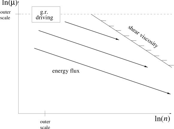
Figure 2: Saturation in the continuum limit. Energy is input to the r-mode at the outer scale of both wavenumber $n$ and frequency $\mu$. Energy then cascades to small $\mu$ and large $n$ along the integral curves $n^{\alpha_{\mu}}\mu^{\alpha_{n}}=$ (const) of the energy flux vector field (20).

In the above “discrete” scenario, the saturation amplitude of the driven mode scales as $A\sim Q_{d}^{-1}$, where $Q_{d}$ is the quality factor of a damped mode. In the “continuum” picture that we now discuss, the saturation amplitude is independent of the linear damping rates, since the energy is transferred by nonlinear interactions. In this cascade picture, both the shape and normalization of the wave energy spectrum are set only by the detailed nonlinear interaction between waves, and the energy input to the system.

How does the cascade arise? Imagine starting with a system in the weak driving limit and adiabatically increasing the driving. When $\gamma_{gr}$ becomes greater than the damping rate $\gamma_{2}+\gamma_{3}$ of the daughter pair with the lowest threshold, the equilibrium solution for that pair is no longer stable and the energy of all three modes will begin to grow. When the energy has grown to the point that additional parametric thresholds are crossed, and if the energy transfer to these pairs is stable, the driven mode will again be saturated. As the driving is increased, this process will continue until many daughter modes are excited with large amplitude. Since linear damping is smaller than driving over a certain range of daughter mode lengthscales, an inertial range has formed where nonlinear forces are dominant. We now proceed to give a heuristic derivation of instability saturation in this continuum case, leaving the detailed derivation appendix A.

Since many modes are excited, we treat the quantum numbers for each mode as a continuum. Introducing the “occupation number” (quasi-particle number) for mode $\alpha$

$$N_{\alpha}=|q_{\alpha}|^{2}/|\omega_{\alpha}|\geq 0,$$ (14)

the mode energy becomes

$$E_{\alpha} = 2E_{\rm unit}|q_{\alpha}|^{2}=2E_{\rm unit}|\omega_{\alpha}|N_{\alpha}.$$ (15)

Eq.6 describes both the fast variation of each individual mode, as well as the slow variation due to nonlinear interactions between modes. We may average over the fast oscillations using the random phase approximation (Zakharov et al. 1992; Kumar & Goldreich 1989; Wu 1998) if the phase randomization time set by the wave dispersion is shorter than the nonlinear interaction timescale. Since the dispersion time is comparable to the mode period for inertial waves, this is equivalent to the weak nonlinearity condition. The resultant kinetic equation for the wave amplitudes is (Zakharov et al. 1992; Kumar & Goldreich 1989)

$$\dot{N}_{\alpha} = I_{\alpha}+\Gamma_{\alpha}N_{\alpha}$$ (16)

where $I_{\alpha}$ represents the rate of change of $N_{\alpha}$ due to nonlinear interactions, and $\Gamma_{\alpha}$ is the rate of driving ($>0$) or damping ($<0$). The interaction term has the form

$$I_{\alpha} = s_{\alpha}\pi\sum_{\beta\gamma}|\kappa_{\alpha\beta\gamma}|^{2}|\omega_{\alpha}\omega_{\beta}\omega_{\gamma}|\delta(\delta\omega_{\alpha\beta\gamma})$$ (17)

$$\times \left(s_{\alpha}N_{\beta}N_{\gamma}+s_{\beta}N_{\gamma}N_{\alpha}+s_{\gamma}N_{\alpha}N_{\beta}\right)$$

where $s_{\alpha}$ is the sign of the frequency of mode $\alpha$.

To proceed further, we must introduce a few properties of the oscillation modes to be derived in section 3. Let $n$, $k$, and $m$ denote the perpendicular (to $\Omega$), parallel, and azimuthal number of nodes, respectively. Since inertial mode oscillation frequencies are proportional to the rotation frequency, we write the mode frequency as $\omega=2\Omega\mu$, where $\mu^{2}\leq 1$ is the dimensionless frequency.

Approximate stationary solutions of eq.16 are found in two steps (see Zakharov et al. (1992) for detailed derivations). First, one ignores the driving and damping, so that the energy flux is conserved. In this case, the energy flux ${\cal F}$ is defined by

$$\omega\int dm\,I \equiv -{\mbox{\boldmath$\nabla$}}_{k}\cdot{\cal F}$$ (18)

where ${\mbox{\boldmath$\nabla$}}_{k}$ is the gradient in momentum space and we have integrated over the $m$ quantum number. In appendix A, we show that stellar inertial waves support a flux of energy to large $n$ and small $\mu$. A schematic drawing of this cascade is given in fig.2. The occupation number for each mode is

$$N = \Omega^{-1}N_{0}n^{-4}|\mu|^{-1/2}\propto n^{-7/2}|k|^{-1/2}$$ (19)

where the normalization constant is related to the fluxes ${\cal F}^{n}$ and ${\cal F}^{\mu}$ in the $n$ and $\mu$ directions, respectively, by

$${\cal F}^{n} = 8\alpha_{n}N_{0}^{2}n^{-1}|\mu|^{-1}\Omega E_{\rm unit}$$

$${\cal F}^{\mu} = -8\alpha_{\mu}N_{0}^{2}n^{-2}\frac{\mu}{|\mu|}\Omega E_{\rm unit}.$$ (20)

The constants $\alpha_{n}$ and $\alpha_{\mu}$ are order unity and positive. A surface of constant energy in momentum space has $\mu\propto n^{8}$, showing that the energy cascades to small frequencies quite rapidly with wavenumber, because of the strong dependence of the coupling coefficients on frequency (see appendix B).

The final step is to match the inertial range solution to the driving range. In other words, we need to find steady state solutions to the equation $I+\gamma_{gr}N=0$, where $\gamma_{gr}$ is the driving rate by gravitational radiation. We approximate $N$ in the driving region by extending the inertial range solution. The power input by the instability is given by

$$\mbox{input power}=\int dn\,dk\,dm\,\gamma_{gr}E$$ (21)

$$\simeq \frac{2}{3}n_{r}^{3}\gamma_{gr}E_{r}=\frac{8}{3}\gamma_{gr}E_{\rm unit}N_{0}n_{r}^{-1}\mu_{r}^{1/2}$$

where the $r$ subscript denotes the driven r-mode and we have approximated the (dimensionless) volume in phase space being driven as $\propto n_{r}^{3}$. The energy escaping the driving region is given by integrating up the flux through each boundary. Roughly, this is given by

output power $$= \int_{\mu_{r}(1-1/n_{r})}^{\mu_{r}}d\mu\ n{\cal F}^{n}$$ (22)

$$+ \int_{n_{r}}^{n_{r}+1}dn\ n|{\cal F}^{\mu}|$$

$$\simeq 8n_{r}^{-1}N_{0}^{2}(\alpha_{n}+\alpha_{\mu})\Omega E_{\rm unit}.$$

Equating the input to output power we can solve for the normalization constant

$$N_{0} = \frac{1}{3}\frac{1}{\alpha_{n}+\alpha_{\mu}}\frac{\gamma_{gr}}{\Omega}\mu_{r}^{1/2}.$$ (23)

Given the normalization, we find

$$\frac{E_{r}}{E_{\rm unit}} = \frac{E(r-mode)}{0.5Mr_{*}^{2}\Omega^{2}}$$ (24)

$$= \frac{2n_{r}^{-4}\mu_{r}}{3(\alpha_{n}+\alpha_{\mu})}\frac{\gamma_{gr}}{\Omega}\equiv\alpha_{e}\frac{\gamma_{gr}}{\Omega}$$

where we parametrize our inexact treatment of the matching condition with the parameter $\alpha_{e}=2n_{r}^{-4}\mu_{r}/3(\alpha_{n}+\alpha_{\mu})$. If we use the quantum numbers of the r-mode, $n_{r}=3$ and $\mu_{r}=1/3$, we find $\alpha_{e}\simeq 4\times 10^{-4}$. However, we choose to be very cautious about this factor since we are extrapolating a WKB treatment into the regime of low order modes . A more conservative estimate would be to set $n_{r}=\mu_{r}=1$, giving $\alpha_{e}\simeq 0.1$. We will use the more conservative result for numerical work in the rest of this paper, but recall that it may overestimate the saturation amplitude by up to three orders of magnitude. Using the r-mode driving rate from eq. 62, the final result for the saturation energy is

$$\frac{E(r-mode)}{0.5Mr_{*}^{2}\Omega^{2}} = 10^{-6}\left(\frac{\alpha_{e}}{0.1}\right)\nu_{\rm khz}^{5}$$ (25)

where $\nu_{\rm khz}$ is the spin frequency in units of $1000\,\rm Hz$.

Why is the saturation amplitude so small? The factor $\gamma_{gr}/\Omega$ is inevitable since the only quantity with the units of frequency in the nonlinear interaction rate is $\Omega$. The numerical factor $\alpha_{e}$ depends on considerations such as the effective volume and area of the driving region, and the power in the driving region relative to the largest scale (energy bearing) waves.

Eq.25 is one of the central results of this paper. It applies when nonlinear energy transfer is faster than linear damping. If nonlinear energy transfer becomes slower than linear damping, the discrete limit of section 2.1 is recovered. Note that the saturation amplitude decreases very rapidly with stellar spin frequency.

3 Oscillation modes in rapidly rotating neutron stars

In this section we discuss the oscillation modes present in rapidly rotating neutron stars. We argue that at the rapid rotation rates of interest for the r-mode instability, the buoyancy and elastic restoring forces can be ignored in comparison with the Coriolis force. The resulting modes which are restored by the Coriolis force are called inertial modes, of which the r-modes are a subset.

3.1 motivation for inertial waves

Within a minute after their birth in a supernova, neutron star cores have become transparent to neutrinos and cooled down sufficiently to form a degenerate gas of neutrons, with a small admixture of electrons and protons determined by beta equilibrium. As shown clearly by Reisenegger & Goldreich (1992), the varying electron fraction $y_{e}\simeq 6.0\times 10^{-3}(\rho/2.8\times 10^{14}\rm\ g\ cm^{-3})$ in the star causes a stable stratification and resulting buoyancy force: Since the neutron pressure $p_{n}\propto[\rho/(1+y_{e})]^{5/3}$, displacing a fluid element upward on timescales slower than the sound crossing time and faster than the timescale of the beta reactions results in the fluid element being heavier than its surroundings, since it came from a region of larger $y_{e}$. An oscillatory motion results, with maximum frequency of order the Brunt-Vaisala frequency (Reisenegger & Goldreich 1992) $N_{bv}\simeq(0.5y_{e}g/H_{p})^{1/2}\simeq 500\,{\rm sec}^{-1}\sim 2\pi\times 100\,\rm Hz$, where $g$ is the local gravity and $H_{p}$ is the local pressure scale height.

The buoyancy force on a fluid element is just $F_{\rm buoy}=-g\delta\rho\simeq-\rho N_{bv}^{2}\xi^{r}$, where $\xi^{r}$ is the radial component of the Lagrangian fluid displacement. The Coriolis force is given by $F_{\rm cor}\sim 2\rho\Omega\omega\xi$, so that the ratio of these two forces for $\omega\sim\Omega$ is roughly

$$\frac{F_{\rm buoy}}{F_{\rm cor}} \sim \left(\frac{N_{bv}}{\Omega}\right)^{2}\sim\left(\frac{100\,\rm Hz}{\nu_{\rm spin}}\right)^{2}.$$ (26)

In a detailed study of the solutions to the fluid perturbation equations for rotating stars including buoyancy, Yoshida & Lee (2000) showed that in the limit of ${F_{\rm buoy}}/{F_{\rm cor}}\gg 1$ the solutions are approximated very well by the r- and g-modes. This limit of large buoyancy force was examined by Morsink (2002) who showed that the nonlinear couplings between r-modes are too small to cause saturation to occur. In the limit of ${F_{\rm buoy}}/{F_{\rm cor}}\ll 1$ Yoshida & Lee (2000) have shown that the solutions of the perturbation equations are well approximated by the inertial modes. As long as we restrict our calculations to stars spinning at a frequency greater than 100 Hz, the inertial modes with zero buoyancy are very good approximation. As we are interested in the possibility of mode saturation at spin frequencies at least as large as 300 Hz, the inertial modes are the most relevant modes and it is possible for us to ignore the buoyancy force as a first approximation. This enables us to find simple solutions for the modes if we further approximate the shape of the star as spherical, a valid approximation for rotation rates well below the breakup rate. However, we expect that the qualitative results found here will hold even in the case when buoyancy is included. The reason is that the approximations made still provide a dense spectrum of modes that may be arbitrarily resonant with the r-mode in the continuum limit. Although the numerical value of the coupling coefficients and damping rates may change because we don’t have exactly the correct shape of the eigenfunctions, we are confident that the essential qualitative features present in our simple example will carry over.

Levin & Ushomirsky (2001) have shown that the elastic restoring force in the neutron star crust becomes small compared to the Coriolis force above a rotation rate of $\sim 50\,\rm Hz$. The net result is that core modes can penetrate into the crust, with only a small discontinuity at the crust-core boundary because of the impedance mismatch. We will ignore crustal elasticity for the remainder of this paper.

We have not included superfluid effects in our calculations. The principal new effect would be dissipation due to mutual friction (the modes themselves are not expected to be changed very much; see, e.g., Lindblom & Mendell (2000)). However, we note that our estimate of the saturation amplitude does not depend on the dissipation rate if an inertial cascade forms (although the outer scale of the inertial range might be affected). Thus, if saturation involves a cascade of energy to numerous inertial modes, we still expect our estimates to hold. Our estimates would change if dissipation via mutual friction is strong enough that only a few modes are excited parametrically. We postpone a thorough examination of this case, which would depend on uncertain mutual friction coefficients, for another paper. However, either way, the saturation amplitude will still be very small.

In the next subsection, we discuss inertial mode eigenfunctions in weakly stratified stars.

3.2 stellar inertial modes

We solve the Euler and continuity equations for adiabatic perturbations of a rotating star. The background star is taken to be spherically symmetric with uniform rotation rate ${\mbox{\boldmath$\Omega$}}=\Omega{\mbox{\boldmath$e$}}_{z}$ and negligible stable stratification. Perturbation modes of the form $\exp(im\phi-i\omega t)$ are found using the Cowling approximation.

The Euler, continuity, and state equations are

$$\rho\ddot{{\mbox{\boldmath$\xi$}}}+2\rho{\mbox{\boldmath$\Omega$}}\times\dot{{\mbox{\boldmath$\xi$}}} = -{\mbox{\boldmath$\nabla$}}\delta p+{\mbox{\boldmath$g$}}\delta\rho$$ (27)

$$\delta\rho+{\mbox{\boldmath$\nabla$}}\cdot\left(\rho{\mbox{\boldmath$\xi$}}\right) = 0$$ (28)

$$\delta p = c^{2}\delta\rho,$$ (29)

where we have ignored terms involving the Brunt-Vaisala frequency

$$N_{bv} = \left(g\frac{d\ln(p^{1/\Gamma_{1}}/\rho)}{dr}\right)^{1/2},$$ (30)

a valid assumption for $\omega\gg N_{bv}$ and $\Omega\gg N_{bv}$. Here we have defined the adiabatic index $\Gamma_{1}$. In this limit, the adiabatic sound speed $c$ and density scale height $H$ are related by $c\simeq(gH)^{1/2}$. Substituting the assumed dependence on $\phi$ and $t$, and eliminating $\delta\rho$, we find that eqns. 27 – 29 become

$${\mbox{\boldmath$\xi$}}+iq\ {\mbox{\boldmath$e$}}_{z}\times{\mbox{\boldmath$\xi$}} = {\mbox{\boldmath$\nabla$}}\psi$$ (31)

$${\mbox{\boldmath$\nabla$}}\cdot{\mbox{\boldmath$\xi$}}+\frac{\omega^{2}}{c^{2}}\psi = \frac{\xi^{r}}{H}.$$ (32)

Here we have replaced the Eulerian pressure perturbation by the quantity $\psi$ defined by $\delta p=\rho\omega^{2}\psi,$ and defined the dimensionless inverse frequency $q=2\Omega/\omega$. We will also heavily use the dimensionless frequency $\mu=1/q=\omega/2\Omega$. We drop the term $\omega^{2}\psi/c^{2}\propto\Omega^{2}/(GM/r_{*}^{3})$ since we are working to leading order in $\Omega$; this is consistent with our assumption that the background star is spherical and suffices to compute the mode functions to leading order in $\Omega$.

The Euler equation 31 can be solved for $\xi$ in terms of $\psi$:

$$\xi = (1-q^{2})^{-1}\left[{\mbox{\boldmath$\nabla$}}\psi-q^{2}{\mbox{\boldmath$e$}}_{z}({\mbox{\boldmath$e$}}_{z}\cdot{\mbox{\boldmath$\nabla$}}\psi)-iq{\mbox{\boldmath$e$}}_{z}\times{\mbox{\boldmath$\nabla$}}\psi\right].$$ (33)

Substituting eq. 33 into the continuity equation 32 gives the wave equation

$${\mbox{\boldmath$\nabla$}}^{2}\psi-q^{2}\frac{\partial^{2}\psi}{\partial z^{2}} = H^{-1}\left(\frac{\partial\psi}{\partial r}-q^{2}\cos\theta\frac{\partial\psi}{\partial z}-\frac{mq}{r}\psi\right).$$ (34)

The boundary condition near the surface is that the Lagrangian change in the pressure vanish, $\Delta p=\delta p+{\mbox{\boldmath$\xi$}}\cdot{\mbox{\boldmath$\nabla$}}p=0$, so that $\delta p\simeq\rho g\xi^{r}$. This is just the statement that the surface layer is hydrostatic, a consequence of the vanishing sound crossing time across a scale height for small depth.

Equation 34 does not appear to be solvable by separation of variables. This motivates us to examine approximate solutions valid for short wavelengths. Our solution generalizes the exact solution of Bryan (1889) for the constant density star; in fact our solution is just Bryan’s solution divided by $\sqrt{\rho}$.

Defining

$$\psi({\mbox{\boldmath$x$}}) = \psi_{0}\left(\frac{\rho_{0}}{\rho}\right)^{1/2}f({\mbox{\boldmath$x$}})$$ (35)

where $\psi_{0}$ is a normalization constant and $\rho_{0}$ is the central density, the differential equation for $f$ is

$${\mbox{\boldmath$\nabla$}}^{2}f-q^{2}\frac{\partial^{2}f}{\partial z^{2}}+{\cal K}^{2}f = 0$$ (36)

with

$${\cal K}^{2} = (1-q^{2}\cos^{2}\theta)\left(\frac{1}{2}\frac{dH^{-1}}{dr}-\frac{1}{4H^{2}}\right)$$ (37)

$$+ \frac{mq}{rH}+\frac{1}{2rH}\left(2-q^{2}\sin^{2}\theta\right).$$

The first two terms in eq. 36 are just the usual differential equation for inertial modes, as derived by Bryan. The compression term $\xi^{r}/H$ in the continuity equation 32 is imaginary in the WKB limit, and leads to the WKB envelope $\rho^{-1/2}$. The definition in eq.35 accounts for this envelope, so that the correction terms in eq.37 are now real. The ${\cal K}^{2}f$ term is most important near the surface, where it scales as $(|{\mbox{\boldmath$k$}}|H)^{-2}$ relative to the other terms in eq.36 ($|{\mbox{\boldmath$k$}}|$ is the local WKB wavenumber). This term describes a slow variation of the wavenumber with position, and is negligible for short wavelength modes. Henceforth, we set ${\cal K}\simeq 0$ in the interior of the star.

The short wavelength approximation breaks down when the vertical wavenumber $k_{r}$ is comparable to the scale height, at about $2k_{r}H\sim 1$, as can be verified directly from eq. 36. When the eigenfunction is constant over a scale height one may picture that the wave attempts to lift an entire scale height of material, which causes reflection. We extend our interior solution to the surface by replacing $\rho$ in eq. 35 with a “cutoff” value $\rho_{cut}$ which becomes constant about one wavelength from the surface.

Figure 3: Surfaces of constant bi-spheroidal coordinate for different values of $q$. The surface of the star is the thick solid line on the unit circle. Only the portions of the spheroids inside this circle are relevant. The short dashed lines represent surfaces of constant bi-spheroidal coordinate $-1/|q|\leq x_{2}\leq 1/|q|$ while the long dashed lines are for the second bi-spheroidal coordinate, which takes on the range $1/|q|\leq x_{1}\leq 1$. The level surfaces are at the values $0.1,0.2,...,0.9$. The surface of the star is described by two coordinate patches, $x_{1}=1/|q|$ near the equator, and $x_{2}=1/q$ near the pole.

Bryan (1889) found a solution to eq.36 for ${\cal K}=0$ in terms of an ingenious bi-spheroidal coordinate system that depends on the frequency $\mu$. Lindblom & Ipser (1999) have given a careful discussion of this coordinate system, paying particular attention to the behavior of the coordinates at the surface of the star. Define the bi-spheroidal coordinates $|\mu|\leq x_{1}\leq 1$ and $-|\mu|\leq x_{2}\leq|\mu|$ by

$$x = r_{*}\left[\frac{(1-x_{1}^{2})(1-x_{2}^{2})}{1-\mu^{2}}\right]^{1/2}\cos\phi$$

$$y = r_{*}\left[\frac{(1-x_{1}^{2})(1-x_{2}^{2})}{1-\mu^{2}}\right]^{1/2}\sin\phi$$

$$z = r_{*}\frac{x_{1}x_{2}}{|\mu|}.$$ (38)

In fig. 3 we plot the surfaces of constant bi-spheroidal coordinate in the $x-z$ plane. In either the $\mu\sim 1$ or $\mu\ll 1$ limits, the surfaces of constant $(x_{1},x_{2})$ are nearly in the $z$ and $R$ directions over most of the star, as one would expect for a local plane wave propagating in the $z$ or $R$ direction. (Here $R$ is the cylindrical radius.) However, the coordinate lines near the point $r\sim r_{*}$ and $\cos\theta=\pm|\mu|$ on the surface of the star vary quite rapidly with respect to $r$ and $\theta$. The result is that the WKB wavenumber becomes quite large near these singular points. (We give a detailed mathematical discussion in appendix B.) As one can see from fig. 3, the coordinate lines come closer to the surface near the singular points, implying the upper turning point is much closer to the surface near the equator (for small $\mu$) than the poles. As a result, the wave amplitudes will be much larger near the equator, as we will now show.

Our approximate solution for the interior of the star is to ignore terms of order $(|{\mbox{\boldmath$k$}}|H)^{-2}$, so that the differential equation becomes

$${\mbox{\boldmath$\nabla$}}^{2}f-q^{2}\frac{\partial^{2}f}{\partial z^{2}} = 0.$$ (39)

Changing to bi-spheroidal coordinates in eq. 39 gives separable differential equations (see Bryan (1889) and Lindblom & Ipser (1999) for details) . Define the solution $f(x_{1},x_{2})=f_{1}(x_{1})f_{2}(x_{2})$ where both $f_{1}$ and $f_{2}$ satisfy

$$\frac{\partial}{\partial x}\left[(1-x^{2})\frac{\partial f}{\partial x}\right]+\left(\kappa^{2}-\frac{m^{2}}{1-x^{2}}\right)f = 0$$ (40)

for separation constant $\kappa^{2}$. This equation has the Legendre function solutions $\kappa^{2}=n(n+1)$, $f_{1}(x_{1})=P_{nm}(x_{1})$ and $f_{2}(x_{2})=P_{nm}(x_{2})$.

The resulting solution for $\psi$ is then

$$\psi({\mbox{\boldmath$x$}},t) = \psi_{0}\left(\frac{\rho_{0}}{\rho}\right)^{1/2}P_{nm}(x_{1})P_{nm}(x_{2})e^{im\phi-i\omega t}.$$ (41)

Note the important fact that this solution is valid for an arbitrary density profile $\rho$, so long as one is safely in the short wavelength limit. This is true even when $\rho$ is not a separable function of $x_{1}$ and $x_{2}$, as is generally the case in the interior since $\rho(r)=\rho\left(\sqrt{1-(x_{1}^{2}-\mu^{2})(\mu^{2}-x_{2}^{2})/\mu^{2}(1-\mu^{2})}\right)$.

The r-modes do not have short wavelengths and hence cannot be described by the above WKB approximation. However, in the leading order approximation of a spherical background star with no buoyancy, the r-mode solutions are given by (Bryan 1889)

$$\psi({\mbox{\boldmath$x$}},t) = \psi_{0}P_{|m|+1,m}(x_{1})P_{|m|+1,m}(x_{2})\exp(im\phi-i\omega t)$$ (42)

$$\propto zR^{|m|}\exp(im\phi-i\omega t)$$

and have frequencies $\mu=-{\rm sign}(m)/(|m|+1)$.

We now derive the WKB limit for the solution in eq. 41. Writing $x_{1,2}=\cos\theta_{1,2}$ and substituting $f\propto\sin^{|m|}\theta\,\exp(i\int^{\theta}d\theta\,k)$ in eq. 40, we find the following standing wave solutions:

$$f(\theta) \simeq \frac{\pi^{-1}}{\sin^{1/2}\theta}\cos(p\theta+\alpha)$$ (43)

where the wavenumber is given by

$$p = \left(n(n+1)-|m|[|m|+1]\right)^{1/2}\simeq n$$ (44)

for $n\gg|m|$ (the WKB limit) and

$$\alpha = -p\pi/2\mbox{ for even parity }$$

$$\alpha = -(p+1)\pi/2\mbox{ for odd parity modes}.$$ (45)

We have chosen to normalize the Legendre polynomials to unity over $4\pi$ steradians. Note that the nodes are spaced evenly in $\theta_{1,2}$. This WKB approximation to the Legendre equation fails within about one wavelength of $\theta=0,\pi$. The $\sin\theta_{1,2}$ factor causes an increase in amplitude toward $\sin\theta_{1,2}=0$. The collected result is then

$$\psi({\mbox{\boldmath$x$}}) = \frac{\psi_{0}}{\pi^{2}}\frac{\cos(p\theta_{1}+\alpha)\cos(p\theta_{2}+\alpha)}{\left(\frac{\rho}{\rho_{0}}\sin\theta_{1}\sin\theta_{2}\right)^{1/2}}e^{im\phi}.$$ (46)

The factor in the denominator $\rho\sin\theta_{1}\sin\theta_{2}\propto\rho R$ is just the mass element, and enforces roughly equal kinetic energy in between each pair of nodes.

An approximate dispersion relation is easily derived using the eigenfunctions of eq.46. The boundary condition is that the compression term $\xi^{r}/H$ in eq. 32 must remain finite as $H\rightarrow 0$, implying $\xi^{r}\rightarrow 0$ in the low frequency approximation. At either surface patch $x_{1}=|\mu|$ or $|x_{2}|=|\mu|$, this condition implies

$$(1-x^{2})\frac{dP_{nm}}{dx}+mP_{nm} = 0$$ (47)

at $x=\pm|\mu|$. Eq.47 is equivalent to the one given by Bryan (1889), as noted by Lindblom & Ipser (1999). The dependence of the frequency and wavenumber on the background stellar model, as discussed by Lockitch & Friedman (1999), is small in the WKB limit. Substituting the WKB expressions gives

$$\sin\theta\tan(p\theta+\alpha) = -\frac{m}{p}.$$ (48)

In the limit $p\gg|m|$, the solutions are found by inspection to be $p\theta+\alpha=-k\pi$, for the mode index $k$. Including the finite $m$ term to first order gives the solution

$$\mu_{nkm} = \omega_{nkm}/2\Omega$$ (49)

$$= \sin(k\pi/p+m/p^{2}-\pi\delta/2p)$$

$$\simeq k\pi/n$$ (50)

where $\delta=0$ for even parity modes and $\delta=1$ for odd parity modes. The $m$ term can be dropped except for the very low frequency, even parity mode with frequency $\mu\simeq m/p^{2}$. All other modes have $\mu\propto p^{-1}$. We find the approximate formula in eq.49 to agree quite well with the exact solutions of eq.47 even for $p$ as small as 5. Lastly, we note that Lockitch & Friedman (1999) have checked the eigenmodes found using bi-spheroidal coordinates with those from a numerical code in spherical coordinates, finding agreement.

We choose to normalize the eigenfunctions so that at unit amplitude ($A=1$) all modes have the same energy, which we call $2E_{\rm unit}$. We can analytically compute the mode energy in the WKB limit where the eigenfunctions are rapidly oscillating ($n\gg m$), with the result

$$E = \omega^{2}\int d^{3}x\,\rho|{\mbox{\boldmath$\xi$}}|^{2}$$ (51)

$$\simeq 4\pi^{-2}\frac{p^{2}\mu^{4}}{(1-\mu^{2})^{3/2}}\rho_{0}\Omega^{2}r_{*}\psi_{0}^{2}.$$

This formula agrees well with numerical integrations. Our normalization convention is that at unit amplitude all modes have the same energy $2E_{\rm unit}$. We then find the value of the normalization constant

$$\psi_{0}^{2} = \frac{E_{\rm unit}}{2\pi^{-2}\frac{p^{2}\mu^{4}}{(1-\mu^{2})^{3/2}}\rho_{0}\Omega^{2}r_{*}}\propto p^{-2}\mu^{-4}.$$ (52)

Modes with rapid spatial variation ($p\gg 1$) or larger frequency $\mu$ have smaller normalization in order for the energy to be the same. As $\mu\rightarrow 1$, the wave amplitude goes to zero since inertial modes do not exist outside this range.

Before moving on to discuss the nonlinear force coefficients, we discuss the normalization integral in eq.51. One can easily find the mode energy to leading order in $\mu$ by setting $\mu=0$ in eq.51. In this limit, the bi-spheroidal coordinates become $x_{1}\simeq(1-R^{2})^{1/2}$ and $x_{2}\simeq 0$. In this limit, the integrand is constant in $z$, and varies as $(1-R^{2})^{-1/2}$ with $R$, which is large near the surface. The kinetic energy then converges as $(1-R^{2})^{1/2}$ from the surface.

4 coupling coefficients

The lowest order nonlinear interaction couples three inertial waves, implying quadratic nonlinear terms as in eq.6. The expressions for the nonlinear force coefficients can be derived either from an action principle (Newcomb 1962; Kumar & Goldreich 1989; Kumar & Goodman 1996) or directly from the equation of motion (Schenk et al. 2002). Note that Schenk et.al. have stressed that the form of the coupling coefficient is the same for rotating systems as for nonrotating systems; only the explicit expressions for the eigenfunctions and background stellar model need be modified. Since we are using daughter modes with wavelengths much smaller than a stellar radius, we keep only the largest term in the coupling coefficient in an expansion of $(|{\mbox{\boldmath$k$}}|H)^{-1}$. For modes ${\mbox{\boldmath$\xi$}}_{1}$, ${\mbox{\boldmath$\xi$}}_{2}$, ${\mbox{\boldmath$\xi$}}_{3}$, the dimensionless coupling coefficient is

$$\kappa_{123} \simeq -\frac{1}{2E_{\rm unit}}\int d^{3}x\left(\xi^{i}_{1}\xi^{j}_{2}\delta p_{3;ij}\right.$$ (53)

$$+ \left.\xi^{i}_{2}\xi^{j}_{3}\delta p_{1;ij}+\xi^{i}_{3}\xi^{j}_{1}\delta p_{2;ij}\right).$$

Since $\delta p\propto\Omega^{2}$, we find that the interaction energy, $\kappa E_{\rm unit}$, scales as the rotational energy of the star. A natural unit of energy is then $E_{\rm unit}=0.5Mr_{*}^{2}\Omega^{2}$. In these units, $A^{2}$ is the mode energy in units of $2E_{\rm unit}=Mr_{*}^{2}\Omega^{2}$.

In section 4.1 we discuss conservation rules for the nonlinear coupling coefficients. Effectively, these rules pick out the largest possible coupling coefficients. The scalings for $\kappa$ are discussed in section 4.2. We confirm a result found in previous studies (Wu & Goldreich 2001) that for waves which satisfy the conservation rules, the coupling coefficients do not become smaller as the daughter mode wavenumber is increased; even though each individual eigenfunction is highly oscillatory, the product is relatively constant. Numerical results are presented in section 4.3 and a detailed analytic calculation is given in appendix B.

4.1 energy and momentum conservation

Figure 4: Coupling coefficient as a function of parent mode quantum number $n_{1}$. The other parent mode quantum numbers are held fixed at $k_{1}=1$ and $m_{1}=2$. The daughter mode quantum numbers $n_{2}$ and $n_{3}$ are allowed to vary, but we have fixed $k_{2}=-2$, $m_{2}=-3$, $k_{3}=-1$, and $m_{3}=1$. The dots show the coupling coefficient determined by numerical integration as described in the text. The line gives the analytic approximation $\kappa_{123}=n_{1}\mu_{1}^{-2}\simeq\pi^{-2}n_{1}^{3}k_{1}^{-2}$.

Consider a parent mode with quantum numbers $(n_{1},k_{1},m_{1})$ and frequency $\mu_{1}$. We are free to choose daughter mode quantum numbers $(n_{2},k_{2},m_{2})$ and $(n_{3},k_{3},m_{3})$ in order to find the largest coupling coefficient (see e.g. Wu & Goldreich (2001)). The integrand is highly oscillatory unless the phases of the waves match at each point in the star. If we expand the standing wave solution in eq.46 in terms of travelling waves, a non-oscillatory integrand implies momentum conservation for the three travelling waves. In addition to conservation of the $m$ quantum number, due to axisymmetry of the background star, we also have momentum conservation along the $\theta_{1}$ and $\theta_{2}$ directions. For small $\mu$, the total number of nodes along $\theta_{1}$ and $\theta_{2}$ simplifies to $N_{1}\sim p\simeq n$ and $N_{2}\sim|\mu|p/\pi\sim k$. The approximate conservation laws which lead to large $\kappa$ can then be written

$$m_{1}+m_{2}+m_{3}=0\ \ \ \mbox{ angular momentum }$$

$$|n_{2}-n_{3}|\mathbin{\lower 3.0pt\hbox{$\hbox to0.0pt{\raise 5.0pt\hbox{$\char 60\relax$}\hss}\mathchar 29208\relax$}}n_{1}\ \ \ \mbox{ momentum along $\theta_{1}$ }$$

$$||k_{2}|-|k_{3}||\mathbin{\lower 3.0pt\hbox{$\hbox to0.0pt{\raise 5.0pt\hbox{$\char 60\relax$}\hss}\mathchar 29208\relax$}}|k_{1}|\ \ \ \mbox{ momentum along $\theta_{2}$ }.$$ (54)

For small frequency, the $\theta_{1}$ and $\theta_{2}$ directions lie nearly along the $R$ and $z$ directions, so that the second and third momentum conservation rules correspond to conservation of momentum along $R$ and $z$. In the limit that the daughter modes have much smaller wavelengths than the parent mode, which will turn out to be the important limit, we find the simple result $n_{2}\simeq n_{3}$ and $|k_{2}|\simeq|k_{3}|$; momentum conservation implies that the daughter modes have momenta of equal magnitude and oppositely directed.

So far, we have used momentum conservation to determine three of the six daughter mode quantum numbers. In order for energy to be efficiently transferred between modes, the interaction must be as nearly resonant as possible, meaning that the detuning is small:

$$\delta\omega=\omega_{1}+\omega_{2}+\omega_{3}\simeq 0.$$ (55)

There are two simple limits of interest. For short wavelength daughter modes with $n_{2}\simeq n_{3}$ and $k_{2}\simeq k_{3}$, one has $\mu_{2}\simeq\mu_{3}\simeq-\mu_{1}/2$; the parent mode interacts with nearly identical daughter modes of half the frequency of the parent. The second solution is where $n_{1}\simeq n_{2}$, and $n_{3}\ll n_{1},n_{2}$. In this case we find $n_{2}\simeq n_{1}+n_{3}$, $k_{2}\simeq k_{1}$, and $k_{3}\simeq k_{1}(n_{3}/n_{1})^{2}$. The frequencies are then $\mu_{2}\simeq-\mu_{1}$ and $\mu_{3}\simeq\mu_{1}(n_{3}/n_{1})\ll\mu_{1}$.

4.2 analytic estimates

Here we give a back of the envelope estimate for the coupling coefficient, leaving the more detailed calculation for appendix B. We will only consider the important limit of short wavelength, nearly identical daughter modes with $\mu_{2}\simeq\mu_{3}\simeq-\mu_{1}/2$. We shall ignore factors of order unity for the present, concentrating only on the scalings. As $\kappa$ is dimensionless, we set $r_{*}=1$ in this section for simplicity.

Incompressibility of the waves implies

$$\kappa\sim\frac{1}{E_{\rm unit}}\int d^{3}x\,\rho\omega_{1}^{2}k_{1z}^{2}\psi_{1}\xi_{2z}^{2}.$$ (56)

For the polytrope of index $1$ we find $\rho\propto r_{*}-r\equiv\hat{z}$ near the surface, where $\hat{z}$ is the distance from the surface. Since the WKB envelope of the waves rises steeply toward the surface, and the factor of $\rho$ cancels the $\rho^{-1}$ from ${\mbox{\boldmath$\xi$}}_{2z}^{2}$, we find that the dominant contribution comes above the turning point for the parent mode, where

$$\psi_{1} \sim \frac{1}{p_{1}\mu_{1}^{2}\hat{z}_{1}^{1/2}}.$$ (57)

Here $\hat{z}_{1}$ is the turning point depth of the parent mode. The daughter mode eigenfunction is strongly peaked in the $\theta$ direction due to the wavenumber

$$k_{2z}\sim\frac{p_{2}\mu_{2}x_{2}}{\left[(\cos^{2}\theta-\mu_{2}^{2})^{2}+8\mu_{2}^{2}\hat{z}\right]^{1/2}}$$ (58)

where $\theta$ is the polar angle in spherical coordinates. The displacement for the daughter mode is then

$$\xi_{2z} \sim \hat{z}^{-1/2}\left[(\cos^{2}\theta-\mu_{2}^{2})^{2}+8\mu_{2}^{2}\hat{z}\right]^{-1/2}.$$ (59)

For $\cos\theta\simeq|\mu_{2}|$, $k_{1z}\simeq p_{1}$ since it is well away from the singularity for mode 1 at $\cos\theta=|\mu_{1}|$. Plugging into eq.56 we find

$$\kappa\sim p_{1}\hat{z}_{1}^{-1/2}\int_{\hat{z}_{2}}^{\hat{z}_{1}}d\hat{z}\int_{-1}^{1}\frac{d(\cos\theta)}{(\cos^{2}\theta-\mu_{2}^{2})^{2}+8\mu_{2}^{2}\hat{z}}.$$ (60)

The integrand has a width $d(\cos\theta)\sim\hat{z}^{1/2}$ and a height $(\mu_{2}^{2}\hat{z})^{-1}$, giving an area $(\mu_{2}^{2}\hat{z}^{1/2})^{-1}$. Using $|\mu_{2}|\sim|\mu_{1}|$ and $\hat{z}_{1}\gg\hat{z}_{2}$, the final result is then

$$\kappa \sim \frac{p_{1}}{\mu_{1}^{2}\hat{z}_{1}^{1/2}}\int_{\hat{z}_{2}}^{\hat{z}_{1}}\frac{d\hat{z}}{\hat{z}^{1/2}}\simeq p_{1}\mu_{1}^{-2}.$$ (61)

The detailed calculation in appendix B confirms that the coefficient is about unity.

We now comment on the scalings for the maximum coupling coefficient in eq.61. The maximum coupling coefficient is found to be independent of the daughter mode quantum numbers. The reason, elucidated by Wu & Goldreich (2001), is that one is integrating over the daughter mode kinetic energy $\rho\mu_{2}^{2}\xi_{2}^{2}$. This quantity is normalized to $2E_{\rm unit}$ when integrated over the whole star, and is roughly $E_{\rm unit}\times\hat{z}_{1}^{1/2}$ when integrated over $0\leq\hat{z}\leq\hat{z}_{1}$. Next, the factor $p_{1}\sim n_{1}$ implies shorter wavelength parent modes interact more strongly. This factor would appear for coupling of local waves in a box. However, the factor $\mu_{1}^{-2}$ would not appear for local waves in a box; it arises from the large peak in the integrand near the surface.

One might wonder whether or not the approximate conservation laws for colliding WKB waves will hold since one is integrating over a small region of the star. The dominant contribution to the integrand comes from a region of size $\hat{z}\sim\hat{z}_{1}\sim|\mu_{1}|/n_{1}$, and the angular size is $d(\cos\theta)\sim\hat{z}^{1/2}\sim(|\mu_{1}|/n_{1})^{1/2}$. The daughter modes have wavelengths $n_{2}$ or $\mu_{2}n_{2}$, depending on direction, so there are still sufficient oscillations in the important region of the star for large enough $n_{2}$.

4.3 numerical calculation

We compute the integral in eq.53 numerically as follows. Choose a point in the star at which to evaluate the integrand. Evaluate $\psi$ and $\delta p$ on the vertices of a Cartesian cube about this point. The derivatives in eq.33 and 53 can then be taken along Cartesian basis vectors , and then appropriate sums over indices taken. The resulting scalar integrand is independent of the coordinate $\phi$ since $m_{1}+m_{2}+m_{3}=0$, so that only a two-dimensional integral over $r$ and $\theta$ remains. We perform this integration with second order accuracy, and increase the number of grid points until the integral converges.

In fig.4, we show the numerical integrations for the coupling coefficient as a function of $n_{1}$, but fixed $k_{1}$ and $m_{1}$. We also fix $(k_{2},m_{2})$ and $(k_{3},m_{3})$ but allow $n_{2}$ and $n_{3}$ to vary. For a given $n_{1}$ we see there is a variation in $\kappa$ due to the degree of momentum conservation. However, the upper envelope set by the maximum coupling coefficient agrees to within $\sim 10\%$ of our analytic formula.

5 damping and driving rates

We review the driving rate by gravitational radiation, and derive simple analytic estimates for the damping rates of inertial modes.

5.1 driving rate

Gravitational radiation reaction is a driving force if the phase velocity in the azimuthal direction is positive in the inertial frame and negative in the rotating frame; otherwise it damps the mode (Friedman & Morsink 1998). The driving rate falls off extremely rapidly with wavenumber, so that only the very lowest modes have an appreciable driving rate compared to damping. Lockitch & Friedman (1999) have computed these driving rates for the inertial modes of a polytrope of index 1, and identified several low order driven modes. However, since the most unstable mode by far is the $(n,k,m)=(3,1,2)$ r-mode, we can ignore all the others to a good approximation.

The driving rate of the $(n,k,m)=(3,1,2)$ r-mode for a polytrope of index 1 with $M=1.4M_{\odot}$ and $r_{*}=12km$ is (Lockitch & Friedman 1999)

$$\gamma_{gr} = 0.05\sec^{-1}\nu_{\rm khz}^{6}.$$ (62)

5.2 bulk viscosity damping

We now compute the damping rate of inertial modes by bulk viscosity damping due to the modified URCA processes. We take the coefficient of bulk viscosity from Sawyer (1989) and Cutler et al. (1990).

The damping rate is

$$-\dot{E}_{bulk} = \int d^{3}x\,\zeta\omega^{2}|{\mbox{\boldmath$\nabla$}}\cdot{\mbox{\boldmath$\xi$}}|^{2}.$$ (63)

The Lagrangian compression is

$${\mbox{\boldmath$\nabla$}}\cdot{\mbox{\boldmath$\xi$}} = \frac{g\xi^{r}}{c^{2}}-\frac{\delta p}{\Gamma_{1}p}\simeq\frac{\xi^{r}}{H}$$ (64)

where the second equality is for low frequency modes. The bulk viscosity coefficient is

$$\zeta = \zeta_{fid}\omega^{-2}T_{9}^{6}\rho^{2}$$ (65)

where

$$\zeta_{fid} = (6\times 10^{25}{\rm g\ cm^{-1}sec^{-3}})(10^{15}{\rm g\ cm^{-3}})^{-2}$$ (66)

$$= 6\times 10^{-5}{\rm g^{-1}cm^{5}sec^{-3}}.$$

Plugging in gives

$$-\dot{E}_{bulk} = \zeta_{fid}T_{9}^{6}\int d^{3}x\,\frac{g^{2}\rho^{4}|\xi_{r}|^{2}}{\Gamma_{1}^{2}p^{2}}.$$ (67)

We will evaluate this integral for a polytrope of index 1. In this case

$$\frac{\Gamma_{1}p}{\rho^{2}} = \frac{GM}{r_{*}\rho_{0}}$$ (68)

is a constant so that

$$-\dot{E}_{bulk} = \zeta_{fid}T_{9}^{6}\left(\frac{\rho_{0}r_{*}}{GM}\right)^{2}\int d^{3}x\,g^{2}|\xi_{r}|^{2}.$$ (69)

In the WKB limit, this integral is logarithmically divergent at $r=r_{*}$ and $\cos\theta=\pm|\mu|$. This divergence implies that equal contributions to the integrand come per decade of distance from the surface. Since the true eigenfunctions flatten off one wavelength from the surface, we cut off the integrals at this distance. Plugging everything into the integral and approximating slowly varying quantities by their surface values gives the amplitude damping rate

$$\gamma_{bulk} = -\frac{\dot{E}_{bulk}}{2E_{\rm unit}}=\frac{1}{8}\zeta_{fid}T_{9}^{6}\frac{\rho_{0}}{r_{*}^{2}\Omega^{2}}\frac{\ln\Lambda}{\mu^{2}},$$ (70)

where $\Lambda=2|\mu|(1-\mu^{2})^{1/2}p$ is roughly the number of nodes along the rotation axis. Evaluating this expression for a fiducial neutron star with polytrope index $n=1$, mass $M=1.4M_{\odot}$ and radius $r_{*}=12{\rm km}$ we find the numerical value

$$\gamma_{bulk} = 1.7\times 10^{-10}\sec^{-1}\ T_{9}^{6}\nu_{\rm khz}^{-2}\frac{\ln\Lambda}{\mu^{2}}.$$ (71)

Note the extremely important fact that this damping rate is very weakly dependent on the wavelength of the mode! The usual picture of a cascade to small scales does not make sense for damping by bulk viscosity. Instead one must carry the energy to small frequency.

For the $(n,k,m)=(3,1,2)$ r-mode, the previously calculated value is (Lindblom et al. 1999)

$$\gamma_{bulk}(r-mode) = 2.8\times 10^{-12}\sec^{-1}T_{9}^{6}\nu_{\rm khz}^{2}.$$ (72)

The r-mode has a different scaling with $\Omega$ and normalization since the compression is smaller: ${\mbox{\boldmath$\nabla$}}\cdot{\mbox{\boldmath$\xi$}}\propto\Omega^{2}$ instead of ${\mbox{\boldmath$\nabla$}}\cdot{\mbox{\boldmath$\xi$}}\propto\xi^{r}/H$.

5.3 shear viscosity

The shear viscosity for nuclear matter has been calculated by Flowers & Itoh (1979), with an analytic fit by Cutler et al. (1990) of the form

$$\nu_{s} = \nu_{s,fid}(\rho/\rho_{0})^{5/4}T_{9}^{-2}$$ (73)

where $\nu_{s,fid}=2000\ {\rm cm^{2}sec^{-1}}(\rho_{0}/10^{15}\ {\rm g\ cm^{-3}})^{5/4}$.

The shear viscosity damping is then

$$-\dot{E}_{shear} = T_{9}^{-2}\int d^{3}x\,\rho\nu_{s}\omega^{2}\left(|\xi_{(i,j)}|^{2}-\frac{1}{3}|{\mbox{\boldmath$\nabla$}}\cdot{\mbox{\boldmath$\xi$}}|^{2}\right)$$ (74)

$$\simeq T_{9}^{-2}\nu_{s,fid}\rho_{0}\omega^{2}\int d^{3}x(\rho/\rho_{0})^{9/4}k^{2}|{\mbox{\boldmath$\xi$}}|^{2}$$

where we have kept terms of leading order in $(|{\mbox{\boldmath$k$}}|H)^{-1}$, and subscripted brackets denote a symmetrized derivative. Plugging everything in, and approximating the density by a power law with depth appropriate for a polytrope of index 1, we find the damping rate

$$\gamma_{shear} \simeq 0.6\pi\frac{p^{2}}{1-\mu^{2}}\frac{\nu_{s,fid}}{r_{*}^{2}}T_{9}^{-2}.$$ (75)

For our fiducial star this becomes

$$\gamma_{shear} = 3.8\times 10^{-9}\sec^{-1}T_{9}^{-2}\frac{p^{2}}{1-\mu^{2}}.$$ (76)

The previously computed r-mode shear damping rate is (Lockitch & Friedman 1999)

$$\gamma_{shear}(r-mode) = 4\times 10^{-9}\sec^{-1}T_{9}^{-2},$$ (77)

which is about a factor of two different from our formula.

As first noted by Bildsten & Ushomirsky (2000), the r-mode is damped much more efficiently by shear in the crust-core boundary layer than by shear over the bulk of the stellar interior. Levin & Ushomirsky (2001) later corrected this damping rate to account for crust with a finite shear modulus. The key parameter is the fractional velocity jump over the boundary layer, called $\eta$. Levin and Ushomirsky found the rate of damping to be

$$\gamma_{vbl}(r-mode) = 1.5\times 10^{-3}\sec^{-1}\eta^{2}\nu_{\rm khz}^{1/2}T_{9}^{-1}$$ (78)

with a realistic estimate for the fractional velocity jump of $\eta\sim 0.1$. Inclusion of the finite shear modulus of the crust gives much better agreement of the r-mode instability curve with the observations of LMXB’s.

We have neglected damping of the daughter modes by shear in the boundary layer.

6 r-mode saturation by discrete modes: the small driving limit

A fundamental plot for the r-mode instability is given in fig.5. The r-mode is unstable for spin frequencies above the thick dashed lines, where $\gamma_{gr}=\gamma_{shear}$, $\gamma_{vbl}$, or $\gamma_{bulk}$. The solid lines show where driving of the r-mode equals damping of daughter modes, indicating marginal stability of the energy transfer. For bulk viscosity, the ratio of driving to damping is

$$\zeta_{b} = \frac{\gamma_{gr}}{\gamma_{bulk}}=8\times 10^{6}\nu_{\rm khz}^{8}T_{9}^{-6}$$ (79)

while for shear viscosity

$$\zeta_{s} = \frac{\gamma_{gr}}{\gamma_{shear}}=1.3\times 10^{7}\nu_{\rm khz}^{6}T_{9}^{2}n^{-2}.$$ (80)

In these estimates we have used $\mu=1/6$, appropriate for daughter modes with the largest coupling coefficients, and $n$ denotes the wavenumber of the daughter mode. Only in the region from the $\zeta_{s}=1$ and $\zeta_{b}=1$ lines to the r-mode instability curve can we possibly have stable energy transfer for the three mode system.

Figure 5: Stability of energy transfer from the r-mode to daughter modes damped by bulk or shear viscosity. The heavy dashed lines show where the r-mode is marginally stable by equating $\gamma_{gr}$ to either $\gamma_{shear}$, $\gamma_{vbl}$ for $\eta=0.1$, or $\gamma_{bulk}$; the r-mode is unstable above these lines. The light solid lines show where $\gamma_{gr}$ equals the bulk ($\zeta_{b}=1$) or shear ($\zeta_{s}=1$) viscosity damping of daughter modes. The three lines $\zeta_{s}=1$ correspond to the number of nodes $n=1,10,100$ from bottom to top. The stability of energy transfer to discrete daughter modes is only stable in the region from the r-mode instability curve (dashed lines) to the $\zeta_{b,s}=1$ lines, i.e., energy transfer to a small number of discrete modes is not stable in the central portion of the r-mode instability region. The nearly vertical dot-dashed line is where bulk viscosity damping equals shear viscosity damping for large lengthscale ($n=1$) mode.

6.1 young neutron stars

Nascent, rapidly rotating neutron stars cool into the region of instability (Owen et al. 1998) at fixed spin frequency. For daughter modes mainly damped by bulk viscosity, there is a narrow region near the instability curve in which energy transfer for a single triplet of modes would be stable. However, in this region, the damping is relatively independent of the daughter mode wavenumber. The quality factor of a daughter mode is roughly

$$Q_{d} \simeq \frac{\omega}{\gamma_{bulk}}\simeq 3.4\times 10^{5}\nu_{\rm khz}^{3}T_{10}^{-6}$$ (81)

where we have used the daughter modes with the largest coupling coefficients so that $\mu_{2,3}=1/6$. We have also set $\ln\Lambda\sim 1$. We found the coupling coefficients are roughly $\kappa\simeq 27$ for a parent mode with $n_{1}=3$ and $\mu_{1}=1/3$ so that the saturation amplitude for a three mode system is given by

$$A_{1}^{2}(bulk) = \frac{E(r-mode)}{0.5Mr_{*}^{2}\Omega^{2}}\simeq\frac{1}{\kappa^{2}Q_{d}^{2}}$$ (82)

$$\simeq 10^{-14}\nu_{\rm khz}^{-6}T_{10}^{12}.$$

This formula would imply that nascent neutron stars cooling into the instability curve after a supernova will saturate at a very small fraction of the rotational energy of the star.

However, this formula is not applicable for the following reason. Since the damping rate of the daughter modes is relatively independent of the daughter mode wavenumber, all daughter modes have essentially the same parametric threshold (roughly eq.82) until $n$ becomes large enough that shear viscosity becomes comparable to bulk viscosity (see fig.5). We estimate this point to be at $n_{b=s}\simeq 10^{4}T_{10}^{4}\nu_{\rm khz}^{-1}$. For daughter modes with frequency $\mu\sim 1/6$, there are roughly $n_{b=s}^{2}\simeq 10^{8}T_{10}^{8}\nu_{\rm khz}^{-2}$ daughter modes parametrically excited to large amplitude by the parent r-mode, so that the discrete limit is not applicable. Thus the r-mode instability in young neutron stars is in the continuum limit discussed in section 7.

6.2 LMXB’s

For the LMXB case, neutron stars with temperature $T\sim 3\times 10^{8}K$ spin up until they hit the instability curve (Bildsten 1998; Levin 1999). When the instability curve near $T_{9}=0.3$ is set by boundary layer shear viscosity with $\eta=0.1$ (Levin & Ushomirsky 2001), we see that if the star stays close to the instability curve, one must go to daughter modes with $10-100$ nodes before the energy transfer can become stable. As a result, $10^{2-4}$ daughter modes will be parametrically excited to large amplitude, and the continuum limit is more appropriate.

If, however, boundary layer shear viscosity is not operating for some reason, then the discrete mode approximation will be valid near the instability curve. The quality factor of the daughter modes in this case is

$$Q_{d} \simeq 5.5\times 10^{9}\nu_{\rm khz}T_{8}^{2}n^{-2}$$ (83)

giving a saturation amplitude for LMXB’s near the instability curve to be

$$A_{1}^{2}(shear) = \frac{E(r-mode)}{0.5Mr_{*}^{2}\Omega^{2}}\simeq\frac{1}{\kappa^{2}Q_{d}^{2}}$$ (84)

$$\simeq 10^{-21}(0.33/\nu_{\rm khz})^{2}T_{8}^{-4}n^{4},$$

which is quite small.

The conclusion we draw in this section is that, for the likely scenario in which either bulk viscosity or boundary layer shear viscosity sets the r-mode instability curve, many modes will be parametrically excited to large amplitude, and the continuum limit discussed in the next section is a better approximation.

7 r-mode saturation in the continuum limit

The saturated r-mode energy was found in section 2.2 to be

$$\frac{E(r-mode)}{0.5Mr_{*}^{2}\Omega^{2}} = 10^{-6}\left(\frac{\alpha_{e}}{0.1}\right)\nu_{\rm khz}^{5}$$ (85)

This solution is valid when there is a clear separation between the inner and outer scales of the turbulence (see Fig. 2). The outer scale is given by the r-mode itself, while the inner scale is where $\gamma_{\rm nl}$, the characteristic rate for amplitude change by nonlinear interactions, is equal to the dissipation rate given by $\gamma_{\rm shear}$ (bulk viscosity is irrelevant for the inner scale; see below). In other words, the inner scale is where the Reynolds number for that scale becomes order unity. We can estimate the nonlinear interaction rate using eqs.16 and 17, with the scalings $n=n_{\alpha}\sim n_{\beta}\sim n_{\gamma}$, $\mu=\mu_{\alpha}\sim\mu_{\beta}\sim\mu_{\gamma}$, etc. We find

$$\gamma_{\rm nl} \sim \frac{I}{N}\simeq\frac{1}{N}\frac{n^{5}}{\mu}(\Omega N)^{2}\sim\gamma_{\rm gr}\frac{n}{n_{r}}\left(\frac{\mu_{r}}{\mu}\right)^{3/2}$$ (86)

where $n_{r}$ and $\mu_{r}$ set the scale for the driving region at which $\gamma_{\rm gr}=\gamma_{\rm nl}$.

The expression for shear viscosity from eq.76 can be written $\gamma_{\rm shear}=\gamma_{s}n^{2}$ in the $\mu^{2}\ll 1$ limit. Equating $\gamma_{\rm nl}$ to $\gamma_{\rm shear}$, we find the inner scale is

$$\frac{n}{n_{r}}\left(\frac{\mu}{\mu_{r}}\right)^{3/2} \simeq n_{r}^{-2}\frac{\gamma_{\rm gr}}{\gamma_{s}}$$ (87)

$$\simeq 170\ n_{r}^{-2}\,\left(\frac{\nu_{\rm spin}}{330\ {\rm Hz}}\right)^{6}T_{8}^{2}.$$

In the region of the $(\Omega,T)$ plane where the right hand side of Eq. (87) is large, many modes are excited with a clear separation between inner and outer scales of turbulence (see Fig. 2). This region includes the entire instability window when the r-mode is damped by a viscous boundary layer. When there is no viscous boundary layer, there is a small region close to the instability curve where (87) is small and where the discrete limit applies instead of the continuum limit.

For bulk viscosity things work differently. The cascade solution will be valid in the region of phase space where $\gamma_{\rm nl}\mathbin{\lower 3.0pt\hbox{$\hbox to0.0pt{\raise 5.0pt\hbox{$\char 62\relax$}\hss}\mathchar 29208\relax$}}\gamma_{\rm bulk}$, or

$$\frac{\mu}{\mu_{r}}\left(\frac{n}{n_{r}}\right)^{2} \mathbin{\lower 3.0pt\hbox{$\hbox to0.0pt{\raise 5.0pt\hbox{$\char 62\relax$}\hss}\mathchar 29208\relax$}} \mu_{r}^{-4}\left(\frac{\gamma_{b}}{\gamma_{\rm gr}}\right)^{2}$$ (88)

$$= 10^{-5}\ \mu_{r}^{-4}\,T_{10}^{12}\,\nu_{\rm khz}^{-16},$$

where we have written $\gamma_{\rm bulk}=\gamma_{b}\mu^{-2}$. In the region of the $(\Omega,T)$ plane where the right hand side of Eq. (88) is large compared to unity, bulk viscosity is dominant at the outer scale and no cascade solution exists. When the right hand side of Eq. (88) is small compared to unity, then a cascade can form, but the bulk viscosity is irrelevant for setting the inner scale of the cascade. We note that the boundary (88) of the bulk viscosity dominated regime approximately coincides with the curve $\zeta_{b}=1$ in Fig. 5. A newly born neutron star will very rapidly move from the instability curve to the $\zeta_{b}=1$ curve at which point the cascade can form.

Finally we note that the weak turbulence approximation which underlies the derivation of Eq. (16) eventually breaks down as one goes to small scales. The weak turbulence approximation requires that the nonlinear energy transfer timescale $1/\gamma_{\rm nl}\sim 20\,{\rm s}\,\nu_{\rm khz}^{-6}n^{-1}\mu^{3/2}$ be much longer than the mode period $\sim 5\times 10^{-4}\,{\rm s}\,\mu^{-1}\nu_{\rm khz}^{-1}$, which breaks down in the regime

$$n\mu^{-5/2}\mathbin{\lower 3.0pt\hbox{$\hbox to0.0pt{\raise 5.0pt\hbox{$\char 62\relax$}\hss}\mathchar 29208\relax$}}4\times 10^{4}\,\nu_{\rm khz}^{-5}.$$ (89)

Thus our turbulent cascade solution of the equations of motion (16) will likely be replaced by some form of strong turbulence at sufficiently small scales. However, this should not affect our prediction of the r-mode’s saturation amplitude, as the regime (89) in phase space where the approximation breaks down is well separated from the driving regime $\mu\sim n\sim 1$.

8 comparison with previous work

There have been three distinct alternative nonlinear mechanisms proposed to saturate the growth of the r-mode: (1) For large amplitude pulsations, the Fermi energies of the electron- proton-neutron gas become significantly shifted, and the kinetic energy can be rapidly converted to both heat and neutrinos by nonlinear bulk viscosity (Reisenegger 2001). (2) The amplitude grows so large ($E\sim E_{\rm rotation}\sim GM^{2}/r_{*}$) that strong shocks occur, rapidly thermalizing the kinetic energy (Lindblom et al. 2001, 2002); (3) In neutron stars with a crust, a turbulent boundary layer forms at the crust-core interface (Wu et al. 2001). We now discuss each in a bit more detail.

Since the Fermi energy of the electron and neutron have a different dependence on density, the Fermi surfaces are shifted out of beta equilibrium when matter is compressed. The scaling of the resulting neutrino emission rate depends on the ratio of chemical potential imbalance, $\Delta\bar{\mu}_{\nu}=\mu_{n}-\mu_{p}-\mu_{e}$, to temperature, which is roughly (Reisenegger 1995)

$$\frac{\Delta\bar{\mu}_{\nu}}{T} \simeq \frac{1}{3}\frac{E_{F,e}}{T}\frac{\Delta\rho}{\rho}$$ (90)

where $E_{F,e}$ is the Fermi energy of the electron. When this ratio is large, $5/8$ of the resulting dissipation heats the star and $3/8$ goes into neutrinos. The rate of such dissipation scales as $\left(\frac{\Delta\bar{\mu}_{\nu}/T}{7.33}\right)^{8}\propto(\Delta\rho/\rho)^{8}$ times the neutrino emissivity of uncompressed matter. The mode damping rate is extremely sensitive to the compression, and can saturate the growth of the r-mode for sufficiently large amplitude. Reisenegger (2001) has done a detailed calculation, finding that the saturation energy is comparable to the stellar rotation energy. This interesting idea gives a larger (less constraining) saturation amplitude compared to the value found in this paper.

Next, Lindblom et al. (2001, 2002) have performed state-of-the-art 3D Newtonian hydrodynamics simulations including a prescription for the radiation reaction force. The only damping mechanism included in the code is numerical viscosity, and of order $128^{3}$ points were used. They were able to follow the linear growth of the r-mode, all the way into the nonlinear regime where $E\geq E_{rot}$. Shocks then formed near the surface of the star, rapidly thermalizing the kinetic energy of the mode.

Since the growth of the instability is so slow compared to the dynamical time in the star, they found it necessary to artificially increase the radiation reaction force by a factor of $\sim 4500$. A natural question is how the mode would saturate if the correct, physical value of the driving force was used. The following physical example is useful to consider. Imagine water waves being driven by wind moving at $1\ {\rm cm\,sec^{-1}}$, a whisper of a breeze, as compared to $4500\ {\rm cm\,sec^{-1}}$, a hurricane. For small amplitude water waves, four wave interactions can transport energy to small scales, saturating the growth of the waves. In a hurricane, the wave growth time is so short that waves grow to large amplitudes and break. Since Lindblom et al. have not addressed how saturation might occur for physical values of either driving or damping of the waves, the relevance of their simulations to saturation of the r-mode instability is not clear.

One comparison which can be made is to use our formula in eq.24 to estimate the saturation amplitude seen in Lindblom et al.’s simulations when $\gamma_{gr}\rightarrow 4500\gamma_{gr}$. We find $E_{\rm simulation}/(0.5Mr_{*}^{2}\Omega^{2})=0.1\left(\alpha_{e}/0.1\right)(4500\gamma_{gr}/\Omega)\simeq 5\times 10^{-3}\left(\alpha_{e}/0.1\right)\nu_{\rm khz}^{5}$. This result can be translated into Lindblom et al.’s notation by using $A_{1}^{2}\simeq 0.5{\tilde{J}}\alpha_{\rm simulation}^{2}=0.008\alpha_{\rm simulation}^{2}$ with the result $\alpha_{\rm simulation}\simeq 0.7\left(\alpha_{e}/0.1\right)^{1/2}\nu_{\rm khz}^{5/2}$. This comparison shows that if one attempted to extrapolate the saturation amplitude over more than three decades in driving force, that the saturation amplitude by mode coupling would indeed be of order unity, in their notation. This does not, of course, explain the saturation amplitude seen in Lindblom et al.’s simulations, which they explain is due to strong shocks near the stellar surface. However, the results of this paper show that their claims of (1) saturation energy of order the rotation energy, and (2) strong shocks as the saturation mechanism, are not supported. They are an artifact of the unphysically large value for the radiation reaction force.

We comment further on the ability of a numerical simulation to accurately reproduce the cascade of energy to small scales as derived in this paper. In simulations with $128^{3}$ points, only a certain number of modes exist because of the finite resolution. Since the detuning is a rapidly decreasing function of wavenumber, secular energy transfer by nearly resonant interactions becomes more important as the number of grid points increases. For instance, daughter modes with half the frequency of the r-mode have quantum numbers in the ratio $k/n\simeq 1/20$, so that one needs nearly $20$ times as many nodes in the cylindrical radius as in the z direction in order to find parametrically excited daughter modes. We estimate that only a few of these might have been accurately modeled by Lindblom et al’s simulations. In time evolutions of the mode amplitude equations with a small number of low order, nonresonant modes (Morsink 2001; Arras 2001), large saturation amplitudes were found as compared to the results in this paper. The reason, as can be clearly seen in eq.9 for the parametric threshold, is that the r-mode cannot easily excite daughter pairs with large detuning. However, going to higher order modes with much smaller detuning can give a saturation amplitude orders of magnitude smaller than for arbitrary, low order modes.

Lindblom et al. specifically commented that three-mode coupling is not the saturation mechanism in section H of their paper. Their claim was based on the lack of power observed in certain modes besides the r-mode during their simulation. However, they focused on interactions which couple the r-mode twice to a third mode. As they themselves comment at the end of section H, they have not included parametric excitation of daughter modes in their constraints. As discussed in section 2.1, couplings of the type discussed by Lindblom et al. (2002) are far less important than parametric couplings, because (1) they are down by a factor of parent mode amplitude, which is small, and (2) only a relatively small region of phase space couples well with the r-mode by non-parametric couplings. Hence, Lindblom et al.’s constraints are not useful since they constrain an unimportant process.

The inability of simulations to include very high order modes presumably also explains the results of the fully relativistic simulations of Font & Stergioulas (2001), in which an r-mode with order unity amplitude was observed not to lose any energy to other modes over several dynamical times. More recent simulations by Gressman et al. (2002) show that for slightly larger initial amplitudes, the r-mode decays rapidly into a differentially rotating configuration without shocks forming. These results are not inconsistent with our analyses, but our results indicate that the r-mode never reaches the regime of rapid nonlinear decay seen by Gressman et al. (2002).

Next we discuss the turbulent boundary layer mechanism of Wu et al. (2001) which operates in neutron stars with a crust. Energy dissipation by turbulent drag scales as $A_{1}^{3}$, leading to saturation of the mode. The attractiveness of this idea is that the turbulent drag force is well understood in magnitude and scaling both from numerical estimates as well as laboratory experiments. These authors considered the effect of such energy dissipation on the crust and thermal history of the star, and go on to discuss the observable spin frequency of the star after it exits the r-mode instability region. For a realistic fractional velocity jump across the crust-core boundary layer, $\eta\sim 0.1$, they found the r-mode saturated at a value $E/(0.5Mr_{*}^{2}\Omega^{2})\simeq 0.2\nu_{\rm khz}^{10}$, which is larger (less constraining) than the value found here, both in normalization, and in the dependence on $\nu_{\rm khz}$. Furthermore, their mechanism does not operate in completely fluid stars without a crust, which is the case for hot young neutron stars.

Lastly, we mention that this paper is a companion paper to that of Morsink (2002), which discusses the nonlinear coupling among r-modes in a star for which buoyancy forces are dominant over Coriolis forces. Morsink found that, because the r-mode frequency decreases with $m$, interactions do not become more resonant as the daughter mode $m$ increase. As a result, energy transfer among three r-modes is not likely to produce a saturation value as low as in this paper.

We conclude that nonlinear mode coupling to inertial modes provides the most stringent constraints on the r-mode amplitude at this time.

9 spin evolution of neutron stars

The spindown torque exerted on the neutron star by gravitational radiation is roughly

$$\tau_{gr} \simeq 0.12\left(\frac{\Omega r_{*}}{c}\right)^{7}\frac{GM^{2}}{r_{*}}A_{1}^{2}$$ (91)

$$\simeq 2\times 10^{42}\,{\rm erg}\,\left(\frac{\alpha_{e}}{0.1}\right)\nu_{\rm khz}^{12}.$$

The spindown time associated with this torque is

$$t_{\rm spindown} \simeq \frac{Mr_{*}^{2}\Omega}{11\tau_{gr}}\simeq 0.01\,{\rm yr}\,\left(\frac{\alpha_{e}}{0.1}\right)^{-1}\nu_{\rm khz}^{-11}$$ (92)

$$\simeq 2\times 10^{3}\,{\rm yr}\,\left(\frac{\alpha_{e}}{0.1}\right)^{-1}\left(\frac{330\,\rm Hz}{\nu}\right)^{11}.$$

Since the spindown rate decreases strongly with spin frequency, most of the time is spent at lower frequencies.

The spindown time becomes $\mathbin{\lower 3.0pt\hbox{$\hbox to0.0pt{\raise 5.0pt\hbox{$\char 62\relax$}\hss}\mathchar 29208\relax$}}10^{4}\ {\rm yr}$ at the lowest rotation rates inside the instability curve, while it is of order a few days for stars rotating near breakup. This is of interest for certain gamma-ray burst models, such as the “supranova” model (Vietri & Stella 1999) in which core collapse leads to ejection of the stellar envelope, as well as a rapidly rotating neutron star which is above the maximum mass for a nonrotating star. Angular momentum transport can then slow the neutron star down, leading to collapse to a black hole and generation of a powerful gamma-ray burst. Our results imply that the gamma-ray burst should occur within of order a week after the supernova explosion.

Next we turn our attention to neutron stars in LMXB’s. The ratio of spindown torque, due to radiation reaction, to accretion torque $\tau_{acc}\simeq\dot{M}(GMr_{*})^{1/2}$ is roughly

$$\frac{\tau_{gr}}{\tau_{acc}} \simeq \frac{2\times 10^{42}(\alpha_{e}/0.1)\nu_{\rm khz}^{12}\ }{10^{34}(\dot{M}/10^{-8}\ M_{\odot}\ {\rm yr^{-1}})}$$ (93)

$$\simeq \frac{10^{-8}M_{\odot}\ {\rm yr^{-1}}}{\dot{M}}\left(\frac{\alpha_{e}}{0.1}\right)\left(\frac{\nu_{\rm spin}}{200\,\rm Hz}\right)^{12}.$$

For accretion rates smaller than the Eddington rate $\dot{M}\simeq 10^{-8}\ M_{\odot}\ {\rm yr}^{-1}$, and spin frequencies above $\nu_{\rm spin}=200\,{\rm Hz}$, the radiation reaction torque is larger than the accretion torque and can halt the further spinup of the neutron star. If the neutron star viscosity is dominated by normal matter, then the star enters into a limit cycle of spinup by accretion and spindown by the r-mode, as discussed by Levin (1999). [The alternative equilibrium scenario is discussed in Sec. 10 below.] Since the r-mode is only likely to be unstable for $\nu_{\rm spin}\mathbin{\lower 3.0pt\hbox{$\hbox to0.0pt{\raise 5.0pt\hbox{$\char 62\relax$}\hss}\mathchar 29208\relax$}}300\,{\rm Hz}$, the r-mode can halt spinup inside the region of instability.

The observable spin frequency is determined by where the star exits the region of r-mode instability, if no other process spins the star down further. The exact spin frequency at which the star exits the region of r-mode instability depends on the evolution of both the spin frequency and the stellar temperature (Levin 1999; Owen et al. 1998; Wu et al. 2001). We can estimate this terminal frequency (Wu et al. 2001) by equating the neutrino cooling luminosity, $L_{\nu}=7.4\times 10^{39}\ T_{9}^{8}\,{\rm erg\,sec}^{-1}$, with the rate of stellar heating due to the r-mode. If we approximate that all the energy input to the r-mode by radiation reaction is damped away as heat, the rate of heating of the star is just given by $\dot{E}_{\rm heat}=2\gamma_{gr}E$, where $E$ is the saturation energy found in eq.85. Equating heating and cooling, we find the equilibrium temperature as a function of spin frequency, given by

$$T_{\rm eq} \simeq 10^{9}\ K\ \left(\frac{\alpha_{e}}{0.1}\right)^{1/8}\left(\frac{\nu_{\rm spin}}{330\,\rm Hz}\right)^{13/8}.$$ (94)

The crystallization temperature of the crust is (Wu et al. 2001) $T_{\rm melt}\sim(5-10)\times 10^{9}\,K$ so the heating by the r-mode cannot prevent the crust from forming when $\nu_{\rm spin}\ll 10^{3}\,{\rm Hz}$. If the instability curve is set by boundary layer shear viscosity ($\gamma_{gr}=\gamma_{vbl}$), the intersection of the equilibrium spin down curve with the r-mode instability curve is given by the terminal frequency

$$\nu_{\rm terminal} \simeq 250\ {\rm Hz}\ \left(\frac{\alpha_{e}}{0.1}\right)^{0.02}\left(\frac{\eta}{0.1}\right)^{0.28}$$ (95)

with a core temperature of roughly

$$T_{\rm terminal} \simeq 6\times 10^{8}\ K\ \left(\frac{\alpha_{e}}{0.1}\right)^{0.15}\left(\frac{\nu_{\rm spin}}{330\,\rm Hz}\right)^{0.46}.$$ (96)

Note that the observable spin frequency is very insensitive to the saturation parameter $\alpha_{e}$, as well as to the fractional velocity jump $\eta$. The spin frequency found in eq.95 is comparable to the lower end of the observed LMXB’s, consistent with a limit cycle (Levin 1999) of spin-up by accretion and spin-down by the r-mode. The timescale to exit the instability curve is roughly $t_{\rm spindown}\simeq 2000\ {\rm yr}\ (330/250)^{11}\ (\alpha_{e}/0.1)^{-1}\simeq 4\times 10^{4}\ {\rm yr}\ (\alpha_{e}/0.1)^{-1}$. This spindown timescale is very sensitive to the position of the instability curve.

For young neutron stars with strong magnetic fields, the spindown torque from magnetic dipole radiation is comparable to that from gravitational radiation. Equating the magnetic dipole spindown timescale (Shapiro & Teukolsky 1983) $t_{\rm md}\simeq 30\,{\rm yr}\,B_{12}^{-2}\nu_{\rm khz}^{-2}$ to $t_{\rm spindown}$, we find that gravitational radiation reaction dominates for frequencies above $\nu_{\rm spin}\simeq 400\,{\rm Hz}\,(0.1/\alpha_{e})^{1/9}\,B_{12}^{2/9}$, where $B_{12}$ is the surface dipole field in units of $10^{12}\ {\rm G}$. Hence for typical pulsars with magnetic fields $\sim 10^{12}{\rm G}$, the spindown torque is dominated by the r-mode only for fairly large spin frequencies.

10 Detectability of gravitational waves

We now discuss the prospect of detecting gravitational waves from r-modes, based on the saturation amplitude (25). We consider three different scenarios: (i) newly born neutron stars where an optically observed extra-Galactic supernova provides the sky location for the gravitational wave search; (ii) LMXB’s in the spinup-spindown limit cycle first discussed by Levin (1999); and (iii) LMXB’s in spin and thermal equilibrium.

For newly born neutron stars, Brady & Creighton (2000) (BC) discuss the detection likelihood by LIGO assuming a large saturation amplitude. They parameterize the saturation amplitude in terms of a parameter $\kappa$ in their Eq. (7.3), which we denote by $\kappa_{bc}$. Our result (25) gives $\kappa_{bc}\simeq 1.2\times 10^{-3}\nu_{\rm khz}^{5}$, while BC took $\kappa_{bc}=1$. In the first year of spindown, $\nu_{\rm khz}$ decreases from $\sim 1$ to $\sim 0.66$ [cf. Eq. (92) above], and thus the gravitational wave strain amplitude will be a factor $\sqrt{\kappa_{bc}}\sim 2.8\times 10^{-2}$ smaller than that considered by BC. The distance to which the source can be seen by enhanced LIGO detectors, for fixed integration time (see below), is correspondingly reduced from BC’s estimate of $\sim 8\,{\rm Mpc}$ to $\sim 200\,{\rm kpc}$, almost inside the Galaxy. Since the galactic supernova rate is roughly once per $50-100\ {\rm yrs}$, the probability that LIGO will detect young neutron stars radiating due to r-modes is small.

We now discuss why we can treat the integration time as fixed. The matched filtering signal to noise ratio $S/N$ for gravitational waves, when averaged over source orientations and polarizations, depends only on the energy per unit frequency $dE/df$ of the waves (Flanagan & Hughes 1998):

$${S^{2}\over N^{2}}={2G\over 5\pi^{2}c^{3}D^{2}}\,\int df\,{1\over f^{2}S_{h}(f)}\,{dE\over df}.$$ (97)

Here $D$ is the distance to the source and $S_{h}(f)$ is the detector noise spectrum. For waves of fixed azimuthal quantum number $m$, using the replacement $dE=2\pi fdJ/m$ yields (Blandford 1984; Lindblom & Owen 2002b)

$${S^{2}\over N^{2}}={4G\over 5\pi mc^{3}D^{2}}\,\int df\,{1\over fS_{h}(f)}\,{dJ\over df},$$ (98)

where $J$ is the $z$-component of angular momentum. As noted by Lindblom & Owen (2002b), the expression (98) is independent of how quickly the star looses angular momentum, and hence of the saturation amplitude. Thus, a priori one would not expect our low saturation amplitude (25) to affect very much the detectability of the signal. The problem however is that it is not possible to integrate long enough to accumulate the total signal-to-noise ratio (98).

Using the stellar model discussed before Eq. (62), the relation $f=4\nu_{\rm spin}/3$ between gravitational wave frequency $f$ and spin frequency, the broadband LIGO-II noise curve from Gustafson et al. (1999), and neglecting the spin dependence of the moment of inertial of the star, we can evaluate (98) for a spindown from an initial spin frequency $\nu_{\rm khz,i}$ in kHz to a final spin frequency $\nu_{\rm khz,f}$. The result is

$${S\over N}=5.4\left({10{\rm Mpc}\over D}\right)\left({1\over\nu_{\rm khz,f}^{2}}-{1\over\nu_{\rm khz,i}^{2}}\right)^{1/2}.$$ (99)

The complete spindown from say $1\,{\rm kHz}$ to $\sim 250{\rm Hz}$ [cf. Eq. (95) above] gives $S/N\sim 21$ at $10\,{\rm Mpc}$. The first year of spindown from $1000\,{\rm Hz}$ to $650\,{\rm Hz}$ [cf. Eq. (92) above] gives instead $S/N\sim 6.2$, which is not too much smaller.

However, the need to perform a search over spindown parameters in practice limits the integration time to $\sim 10^{6}$ seconds. BC analyzed the performance of a “stack slide” search method, involving demodulating the signal for many different choices of spindown parameters, dividing the demodulated data into several chunks or “stacks”, computing the power spectrum of each stack and adding the power spectra. The threshold value $\rho_{\rm th}$ of $S/N$ for this method, assuming $1\%$ false alarm probability, is approximately given by solving the equation

$$\Gamma(N_{s},N_{s}+\rho_{\rm th}^{2}/4)/\Gamma(N_{s})=0.01/(N_{b}N_{p}).$$ (100)

where $\Gamma(a,b)$ is the incomplete gamma function, $N_{s}$ is the number of stacks, $N_{b}$ is the number of frequency bins per stack, and $N_{p}$ is the number of points in the space of spindown parameters. BC’s estimate that r-modes are detectable out to $8\,{\rm Mpc}$ was based on assuming a Teraflop of computing power, which implied an optimum detection strategy of $\sim 8$ stacks of $\sim 10^{5}$ s duration each, integrating from $\nu_{\rm spin}=200\,{\rm Hz}$ to $\nu_{\rm spin}\sim 186\,{\rm Hz}$.

We can modify the BC analysis for our turbulent cascade scenario as follows. Optimum sensitivity is achieved late in the spindown, so we assume that $\nu_{\rm spin}\sim 650\,{\rm Hz}$, corresponding to 1 year after the start of the spindown if the initial spin frequency is 1 kHz. We take the parameter values $\mu_{\rm max}=0.3$, $f_{\rm max}=(4/3)650{\rm Hz}$ (instead of $200\,{\rm Hz}$ as in BC), and a spindown timescale $\tau_{\rm min}=1\,{\rm yr}$, which from Eq. (92) is appropriate after 1 year of spindown. Maximizing over the number of stacks and stack durations as in BC gives that the optimum detection strategy for a Teraflop of computing power is to use $\sim 10$ stacks of duration $\sim 3\times 10^{4}$ s each. The corresponding number of parameter space points is $N_{p}\sim 6\times 10^{8}$, from Eq. (2.20) of BC, which gives from Eq. (100) a threshold value of $\rho_{\rm th}\sim 15$. Combining this with Eq. (99), and noting that at $\nu_{\rm spin}\sim 650{\rm Hz}$ an integration time of $3\times 10^{5}$ s corresponds to $\Delta\nu_{\rm spin}\sim 0.5(\alpha_{e}/0.1)\,{\rm Hz}$ gives that the source would be detectable to $\sim 200(\alpha_{e}/0.1)^{1/2}\,{\rm kpc}$, consistent with our earlier estimate.

This conclusion, however, is based on the assumption of using the stack-slide search method. It is conceivable that an alternative signal processing strategy (and increased computational power) might enable one to integrate for longer periods and achieve a sensitivity closer to the original BC estimate.

We mention in passing another possible difficulty in searching for the signal from r-modes when a turbulent cascade is present. This difficulty is that the phase of the r-mode will wander randomly in time due to the interaction with the turbulent cascade, on some timescale $t_{\rm c}$. The peak in the Fourier transform of the demodulated data stream will correspondingly be smeared out over a frequency interval of width $\sim 1/t_{\rm c}$, which will be over several frequency bins if the stack size is larger than $t_{\rm c}$.

The phase coherence timescale for a typical mode in the cascade will be of order

$$t_{c}\sim{1\over\gamma_{\rm nl}},$$ (101)

or smaller, where $\gamma_{\rm nl}$ is the the nonlinear energy transfer rate (86) (Zakharov et al. 1992). For the r-mode this is only $\sim 200\,{\rm s}$ at $\nu_{\rm spin}\sim 700{\rm Hz}$. However, one might expect the coherence time of the r-mode to be somewhat longer than the estimate (101), since the r-mode is being pumped coherently and is loosing energy by interacting simultaneously with a large number of different modes. Unless the phase coherence time for the r-mode is $10^{2}-10^{3}$ times larger than the estimate (101), the sensitivity of the search will be reduced. Again, it may be possible to modify the data analysis procedure to compensate for the phase wandering .

Next, we consider the detectability of r-modes in LMXB’s in the spin up/spin down limit cycle. The signal from the spin down phase is essentially the same as for newborn neutron stars, except that they will typically be seen at a low frequency where most of the spindown time is spent. At lower spin frequencies the search over spin-down parameters becomes significantly easier, since the spindown timescale is longer. The formula (4.3) in BC for computational power, with $f_{\rm max}=\nu_{\rm spin}$ and $\tau_{\rm min}$ given by Eq. (92), shows that for $\nu_{\rm spin}\mathbin{\lower 3.0pt\hbox{$\hbox to0.0pt{\raise 5.0pt\hbox{$\char 60\relax$}\hss}\mathchar 29208\relax$}}400\,{\rm Hz}$ integration times as long as $10^{7}$ s can be achieved with 1 Teraflop of computing power. Combining Eqs. (92) and (99) gives that the signal to noise ratio for a $10^{7}$ s integration starting at $\nu_{\rm spin}$ is

$${S\over N}\sim 9\left({\nu_{\rm spin}\over 330\,{\rm Hz}}\right)^{9/2}\,\left({100\,{\rm kpc}\over D}\right)\,\left({\alpha_{e}\over 0.1}\right)^{1/2}.$$ (102)

In the regime $\nu_{\rm spin}\lesssim 400{\rm Hz}$, the signal-to-noise threshold from the BC method is $\rho_{\rm th}\sim 10$, within a factor of $\sim 2$, giving that the signal should be visible to a distance

$$D\sim 90\,{\rm kpc}\,\left({\nu_{\rm spin}\over 330\,{\rm Hz}}\right)^{9/2}\left({\alpha_{e}\over 0.1}\right)^{1/2}$$ (103)

for $\nu_{\rm spin}\lesssim 400\,{\rm Hz}$.

However, as noted by Levin (1999), the chance of observing a particular source emitting gravitational waves is proportional to the relative length of time spent in the spindown phase of the limit cycle. Using our saturation amplitude we find a duty cycle $\sim 10^{-3}(0.1/\alpha_{e})$, implying that one would need of order $10^{3}(\alpha_{e}/0.1)$ LMXB’s within the distance (103) in order to overcome the small duty cycle. Nevertheless, as argued by Heyl (2002), there may be enough Galactic LMXB’s that some will be seen in the spin-down phase by enhanced LIGO, especially if $\alpha_{e}$ is smaller than $0.1$.

We note that for LMXB’s, the phase wandering of the r-mode due to the turbulent cascade is less of a problem, since the nonlinear energy transfer timescale (86) increases rapidly as $\nu_{\rm spin}$ decreases. There is in addition a phase wandering due to fluctuations in the accretion torque, but this occurs over much longer timescales and can be dealt with in the manner suggested by BC.

The third possibility we consider is when the viscosity of an accreting star is independent of temperature or is an increasing function of temperature. In such a case the star can achieve an equilibrium state where the accretion spin-up torque is stably balanced by the radiation reaction torque due to the r-mode, and r-mode heating is balanced by neutrino cooling (Levin 1999). Such equilibria have been found for stars with hyperon cores (Wagoner 2002) and for strange stars (Andersson, Jones & Kokkotas 2001). [However, the central densities of neutron stars are sufficiently uncertain that hyperon cores may or may not exist.] In these scenarios, the equilibrium r-mode amplitude is not set by the turbulent cascade considered here, but instead by the equilibrium conditions. The gravitational wave signal is weaker than the limit cycle case considered above, and its strength can be inferred from the X-ray flux (Bildsten 1998).

11 conclusions

In this paper, we have accomplished several objectives, which can be divided into stellar oscillation theory, and phenomenology of neutron star spin evolution.

We have, for the first time, presented a WKB theory of global stellar inertial modes (section 3 and appendix B), including both the rapidly varying phase and amplitude which rises quickly toward the surface. Both the eigenmodes and pulsation frequencies take on a very simple form, which was never clearly elucidated in previous calculations [e.g., Lindblom & Ipser (1999); Lockitch & Friedman (1999).] Appendix B gives a detailed mathematical treatment of inertial waves. We have estimated when the affects of buoyancy become important. The damping rates by bulk and shear viscosity appropriate for neutron stars have been derived in section 5, and reduced to simple, accurate formulae giving the scalings with stellar parameters and mode quantum numbers.

Next, we have given a complete review of saturation of an overstable mode in the two different limits of strong and weak driving force. The literature for the weak driving limit, familiar from studies of main sequence or white dwarf pulsators (Dziembowski & Krolikowska 1985; Wu & Goldreich 2001), is reviewed in detail, and shown not to apply to most physical situations in which the r-mode instability operates. The strong driving limit, in which a turbulent cascade forms, has never been applied to stellar oscillations to our knowledge. Therefore, the weak turbulence methods in this paper may find application for amplitude saturation in stars with a driving force strong enough to parametrically excite many modes, but weak enough that shocks do not form. In the strong driving limit, we find that the r-mode saturates at an energy $E/E_{rotation}\ll\gamma_{gr}/\Omega$.

The consequences of these calculations for neutron star spin evolution are as follows. First, the time scale for a rapidly rotating ($10^{3}\,\rm Hz$) young neutron star to spin down to a frequency $\nu_{\rm spin}$ by gravitational radiation spindown torque is $t_{\rm spindown}\simeq 2\times 10^{3}\,{\rm yr}\,(\alpha_{e}/0.1)^{-1}(\nu_{\rm spin}/{330\,\rm Hz})^{-11}$. Hence, the r-mode can be responsible for an initial, rapid spindown, but magnetic dipole radiation will dominate for spin frequencies below $\nu_{\rm spin}\simeq 400\,{\rm Hz}\,(0.1/\alpha_{e})^{1/9}\,B_{12}^{2/9}$. Second, in spite of the small saturation amplitude, we find that the gravitational radiation spin-down torque is still sufficiently large to halt the spin-up by accretion for neutron stars in LMXB’s. Hence, our calculation confirms the validity of this assumption by previous investigators. If the viscosity is dominated by normal matter, the star will enter into the limit cycle in spin and temperature discussed by Levin (1999). Finally, we estimate that newly born neutron stars will be visible to $\sim 200(\alpha_{e}/0.1)^{1/2}\,{\rm kpc}$ with enhanced LIGO interferometers, and LMXB’s in the spin down phase of the Levin limit cycle out to $\sim 90\,(\nu_{\rm spin}/330\,{\rm Hz})^{9/2}(\alpha_{e}/0.1)^{1/2}\,{\rm kpc}$ for $\nu_{\rm spin}\mathbin{\lower 3.0pt\hbox{$\hbox to0.0pt{\raise 5.0pt\hbox{$\char 60\relax$}\hss}\mathchar 29208\relax$}}400\,{\rm Hz}$.

Appendix A cascade solution

In this appendix we find scale-free solutions to the kinetic equation 17. The material in this appendix can be found in texts on weak turbulence theory, e.g. Zakharov et al. (1992), section 3.3. For convenience we use dimensionless units with $E_{\rm unit}=1$ and $\Omega=1$.

We approximate the mode frequency as $\omega=2\mu\simeq 2\pi k/n=s2\pi|k|/n$, where $s=\pm 1$ is the sign of the frequency. For notational simplicity, we will use both $k$ and $\mu$ as positive numbers for the following derivation, using $s$ to take into account the sign. The resulting expression will then be written in a form valid for either positive or negative $\mu$. The sum over modes is then given by

$$\sum_{\alpha} \simeq \sum_{n=0}^{\infty}\sum_{k=-n/\pi}^{n/\pi}\sum_{m=-n}^{n}\simeq\pi^{-1}\sum_{s=\pm 1}\int_{0}^{\infty}dn\,n\int_{0}^{1}d\mu\int_{-n}^{n}dm.$$ (A1)

Here we used $\mu=\pi k/n$ instead of $k$ since $k$ has an implicit scaling with $n$. The coupling coefficients are assumed to be negligible if momentum conservation is not satisfied, so that

$$|\kappa_{\alpha\beta\gamma}|^{2} \simeq |\bar{\kappa}_{\alpha\beta\gamma}|^{2}\delta(s_{\alpha 1}n_{\alpha}+s_{\beta 1}n_{\beta}+s_{\gamma 1}n_{\gamma})\delta(s_{\alpha 2}k_{\alpha}+s_{\beta 2}k_{\beta}+s_{\gamma 2}k_{\gamma})\delta(m_{\alpha}+m_{\beta}+m_{\gamma}).$$ (A2)

The signs $s_{\alpha 2}$ etc. allow for waves moving in either direction (see appendix B). We use the fact that the coupling coefficient is approximately independent of both $m$ and the sign of $\mu$, and is separately scale invariant in $n$ and $\mu$ to say

$$\bar{\kappa}_{\alpha\beta\gamma} = \bar{\kappa}(n_{\alpha},\mu_{\alpha},n_{\beta},\mu_{\beta},n_{\gamma},\mu_{\gamma})$$

$$\bar{\kappa}(an_{\alpha},b\mu_{\alpha},an_{\beta},b\mu_{\beta},an_{\gamma},b\mu_{\gamma}) = a^{u}b^{v}\bar{\kappa}(n_{\alpha},\mu_{\alpha},n_{\beta},\mu_{\beta},n_{\gamma},\mu_{\gamma}).$$ (A3)

In appendix B we show that $u=1$ and $v=-2$. Since the mode frequencies and coupling coefficients are approximately independent of the $m$ quantum numbers, the $m$ dependence can be integrated over giving the function

$$A(n_{\alpha},n_{\beta},n_{\gamma}) = \int_{-n_{\alpha}}^{n_{\alpha}}dm_{\alpha}\int_{-n_{\beta}}^{n_{\beta}}dm_{\beta}\int_{-n_{\gamma}}^{n_{\gamma}}dm_{\gamma}\,\delta(m_{\alpha}+m_{\beta}+m_{\gamma}).$$ (A4)

This function is symmetric, and is $A\simeq 4n_{\alpha}n_{\beta}$ in either the limit $n_{\alpha}\ll n_{\beta}\simeq n_{\gamma}$ or $n_{\beta}\ll n_{\alpha}\simeq n_{\gamma}$.

Plugging these definitions into eq.17, and summing over the frequency signs we find

$$\int dm_{\alpha}\,I_{\alpha}=\pi(2/\pi)^{2}\int dn_{\beta}\,n_{\beta}dn_{\gamma}\,n_{\gamma}d\mu_{\beta}\,d\mu_{\gamma}\ A|\bar{\kappa}_{\alpha\beta\gamma}|^{2}\mu_{\alpha}\mu_{\beta}\mu_{\gamma}\delta(\delta n)\delta(\delta k)N_{\alpha}N_{\beta}N_{\gamma}$$ (A5)

$$\times \left[\left(\frac{1}{N_{\alpha}}-\frac{1}{N_{\beta}}-\frac{1}{N_{\gamma}}\right)\delta(\mu_{\alpha}-\mu_{\beta}-\mu_{\gamma})-\left(\frac{1}{N_{\beta}}-\frac{1}{N_{\gamma}}-\frac{1}{N_{\alpha}}\right)\delta(\mu_{\beta}-\mu_{\gamma}-\mu_{\alpha})\right.$$

$$- \left.\left(\frac{1}{N_{\gamma}}-\frac{1}{N_{\alpha}}-\frac{1}{N_{\beta}}\right)\delta(\mu_{\gamma}-\mu_{\alpha}-\mu_{\beta})\right].$$

We attempt to find scale-free inertial range solutions of the form

$$N = N_{0}n^{-p}\mu^{-q}.$$ (A6)

After inserting this power law dependence on $n$ and $\mu$ into the eq.A5, one can make a change of coordinates in the second and third sets of terms in the last parenthesis, in order to make them have the same form as the first term, up to a scaling factor. For instance, in the second set of terms let $n_{\beta}=n_{\alpha}^{2}/n_{\beta^{\prime}}$, $\mu_{\beta}=\mu_{\alpha}^{2}/\mu_{\beta^{\prime}}$, $n_{\gamma}=n_{\gamma^{\prime}}n_{\alpha}/n_{\beta^{\prime}}$, and $\mu_{\gamma}=\mu_{\gamma^{\prime}}\mu_{\alpha}/\mu_{\beta^{\prime}}$. After simplifying and collecting terms we find

$$\int dm_{\alpha}\,I_{\alpha}=\pi N_{0}^{2}(2/\pi)^{2}\int dn_{\beta}\,n_{\beta}dn_{\gamma}\,n_{\gamma}d\mu_{\beta}\,d\mu_{\gamma}\ A|\bar{\kappa}_{\alpha\beta\gamma}|^{2}\mu_{\alpha}\mu_{\beta}\mu_{\gamma}\delta(\delta n)\delta(\delta k)\delta(\mu_{\alpha}-\mu_{\beta}-\mu_{\gamma})$$ (A7)

$$\times (n_{\alpha}n_{\beta}n_{\gamma})^{-p}(\mu_{\alpha}\mu_{\beta}\mu_{\gamma})^{-q}\left(n_{\alpha}^{p}\mu_{\alpha}^{q}-n_{\beta}^{p}\mu_{\beta}^{q}-n_{\gamma}^{p}\mu_{\gamma}^{q}\right)$$

$$\times \left[1-\left(\frac{n_{\alpha}}{n_{\beta}}\right)^{2(p_{0}-p)}\left(\frac{\mu_{\alpha}}{\mu_{\beta}}\right)^{2(q_{0}-q)-1}-\left(\frac{n_{\alpha}}{n_{\gamma}}\right)^{2(p_{0}-p)}\left(\frac{\mu_{\alpha}}{\mu_{\gamma}}\right)^{2(q_{0}-q)-1}\right]$$

where $p_{0}=u+3$ and $q_{0}=v+5/2$. We can make the scaling of eq.A7 with $n_{\alpha}$ and $\mu_{\alpha}$ explicit by defining $x_{\beta}=n_{\beta}/n_{\alpha}$, $x_{\gamma}=n_{\gamma}/n_{\alpha}$, $y_{\beta}=\mu_{\beta}/\mu_{\alpha}$, $y_{\gamma}=\mu_{\gamma}/\mu_{\alpha}$, $\kappa_{\alpha\beta\gamma}=n_{\alpha}^{u}\mu_{\alpha}^{v}f_{\alpha\beta\gamma}$, and $\bar{A}=A/n_{\alpha}^{2}$. We find

$$\int dm_{\alpha}\,I_{\alpha} = 4N_{0}^{2}n_{\alpha}^{2(p_{0}-p)-2}\mu_{\alpha}^{2(q_{0}-q)-2}{\cal I}(p,q)$$ (A8)

where ${\cal I}(p,q)$ is the dimensionless integral

$${\cal I}(p,q) = \int dx_{\beta}\,x_{\beta}dx_{\gamma}\,x_{\gamma}dy_{\beta}\,dy_{\gamma}\,\bar{A}f^{2}_{\alpha\beta\gamma}y_{\beta}y_{\gamma}\delta(\delta x)\delta(\delta xy)\delta(\delta y)(x_{\beta}x_{\gamma})^{-p}(y_{\beta}y_{\gamma})^{-q}\left(1-x_{\beta}^{p}y_{\beta}^{q}-x_{\gamma}^{p}y_{\gamma}^{q}\right)$$ (A9)

$$\times \left(1-x_{\beta}^{2(p-p_{0})}y_{\beta}^{2(q-q_{0})+1}-x_{\gamma}^{2(p-p_{0})}y_{\gamma}^{2(q-q_{0})+1}\right).$$

Stationary solutions to eq. A7 are now easily found by using the delta functions to force either the first or second parenthesis to zero (Zakharov et al. 1992). For instance, using the frequency delta function to set the first parenthesis to zero gives $N\propto\mu^{-1}$, so that all modes have the same energy, i.e., thermodynamic equilibrium. Using the momentum delta functions to set the first parenthesis to zero gives thermodynamic equilibria with respect to a moving reference frame. Setting the second parenthesis to zero using the momentum delta functions gives solutions supporting a constant momentum flux. We are interested in solutions which support an energy flux. The frequency delta function can be used to set the second parenthesis to zero if we let $p=p_{0}=u+3=4$ and $q=q_{0}=v+5/2=1/2$. We now proceed to show that this solution corresponds to a flux of energy to small frequency and large wavenumber.

In the inertial range, driving and damping are negligible, and the conserved energy flux has components ${\cal F}^{n}$ and ${\cal F}^{\mu}$ which satisfy

$$\omega_{\alpha}\int dm_{\alpha}\,I_{\alpha}+{\mbox{\boldmath$\nabla$}}_{k}\cdot{\bf{\cal F}}_{\alpha} = \omega_{\alpha}\int dm_{\alpha}\,I_{\alpha}+\frac{1}{n}\frac{\partial}{\partial n}\left(n{\cal F}^{n}_{\alpha}\right)+\frac{\partial{\cal F}^{\mu}_{\alpha}}{\partial\mu}=0.$$ (A10)

Care must be taken in evaluating eq.A8. For finite values of $n_{\alpha}$ and $\mu_{\alpha}$, taking the limit $(p,q)\rightarrow(p_{0},q_{0})$ gives $\int dm_{\alpha}\,I_{\alpha}=0$. However, in the vicinity of $n_{\alpha}=0$ or $\mu_{\alpha}=0$ eq.A8 takes on the indeterminate form $0/0$, since ${\cal I}\rightarrow 0$ in the numerator and either $n_{\alpha}$ or $\mu_{\alpha}$ goes to zero in the denominator. Following Zakharov et.al., we evaluate this expression using the delta function representation $\mbox{lim}_{\epsilon\rightarrow 0}\epsilon|x|^{\epsilon-1}=2\delta(x)$ to find

$$\mu_{\alpha}n_{\alpha}\int dm_{\alpha}\,I_{\alpha} = -4N_{0}^{2}\left(\frac{1}{\mu_{\alpha}}\frac{\partial{\cal I}}{\partial p}(p_{0},q_{0})\delta(n_{\alpha})+\frac{1}{n_{\alpha}}\frac{\partial{\cal I}}{\partial q}(p_{0},q_{0})\delta(\mu_{\alpha})\right).$$ (A11)

Hence, the flux can only have a source for $n=0$ or $\mu=0$. Plugging eq.A11 into eq.A10, using $\omega=2\mu$, and integrating over $n$ or $\mu$, respectively, gives the two components of the flux

$${\cal F}^{n} = 8N_{0}^{2}n^{-1}\mu^{-1}\frac{\partial{\cal I}}{\partial p}(p_{0},q_{0})$$

$${\cal F}^{\mu} = 8N_{0}^{2}n^{-2}\frac{\partial{\cal I}}{\partial q}(p_{0},q_{0}).$$ (A12)

We now estimate the dimensionless flux integrals, verifying that they converge and give have the correct sign. We do this by breaking the integration up into two regimes: large daughter mode wavenumber ($x_{\beta}\gg 1$) and small daughter mode wavenumber ($x_{\beta}\ll 1$). Although our expansions for the integrand are technically only valid in the respective limits, we extend them all the way to $x_{\beta}\sim 1$.

When the derivatives with respect to $p$ and $q$ are taken in eq.A9, only the last parenthesis need be differentiated since it gives zero for $(p,q)=(p_{0},q_{0})$. The coupling coefficients for the two limits are given in appendix B. The resulting expressions are

$$\frac{\partial{\cal I}}{\partial p}(p_{0},q_{0}) \simeq 2^{3/2}\int_{1}^{\infty}dx_{\beta}x_{\beta}^{-2}\ln x_{\beta}+\frac{128}{\pi^{3}}\int_{0}^{1}dx_{\beta}x_{\beta}^{1/2}\left(\ln x_{\beta}+1\right)$$ (A13)

$$= 2^{3/2}+\frac{256}{9\pi^{3}}\simeq 3.7\equiv\alpha_{n}$$

and

$$\frac{\partial{\cal I}}{\partial q}(p_{0},q_{0}) = -2^{3/2}\ln{2}\int_{1}^{\infty}dx_{\beta}x_{\beta}^{-2}+\frac{128}{\pi^{3}}\int_{0}^{1}dx_{\beta}x_{\beta}^{1/2}\ln x_{\beta}$$ (A14)

$$= -2^{3/2}\ln{2}-\frac{512}{9\pi^{3}}=-3.8\equiv-\alpha_{\mu}.$$

We note that the contribution to ${\cal F}^{n}$(${\cal F}^{\mu}$) from both large and small $x_{\beta}$ are positive (negative).

The energy flux is toward larger $n$ and smaller $\mu$. We now restore the sign of $\mu$ in order to have an expression valid for either sign. The final result for the energy flux is then

$${\cal F}^{n} = 8\alpha_{n}N_{0}^{2}n^{-1}|\mu|^{-1}$$

$${\cal F}^{\mu} = -8\alpha_{\mu}N_{0}^{2}n^{-2}\frac{\mu}{|\mu|}.$$ (A15)

We also note the final answer for the occupation number

$$N = N_{0}n^{-4}\mu^{-1/2}$$ (A16)

where $N_{0}$ is related to the energy flux by eq.A15.

Appendix B analytic estimate of the maximum coupling coefficient

Here we give a detailed analytic calculation of the maximum coupling coefficient. We make the following approximations: (1) $n\gg m$, the WKB limit; (2) $k_{\phi}\ll k_{R}$, which follows from (1); (3) short wavelength daughter modes with $\mu_{\beta}\simeq\mu_{\gamma}\simeq-\mu_{\alpha}/2$; (4) an $n=1$ polytropic background star. For convenience, we use units with $r_{*}=M=1$, and we use the normalization condition $E_{\rm unit}=0.5Mr_{*}^{2}\Omega^{2}$. In these units, the density profile near the surface is $\rho=\rho_{0}\hat{z}$, where the central density is $\rho_{0}=\pi/4$.

We decompose $\psi$ in eq.46 as a sum of plane waves as

$$\psi({\mbox{\boldmath$x$}}) = \frac{\psi_{0}}{(2\pi)^{2}}\left(\frac{\rho}{\rho_{0}}\sin\theta_{1}\sin\theta_{2}\right)^{-1/2}\sum_{s_{1},s_{2}=\pm 1}\exp(i\chi_{s_{1}s_{2}})$$ (B1)

where the WKB phase is

$$\chi_{s_{1}s_{2}} = p(s_{1}\theta_{1}+s_{2}\theta_{2})+m\phi+\alpha(s_{1}+s_{2}).$$ (B2)

In the small $\mu$ limit, we can write $\theta_{2}\simeq\pi/2-|\mu|\epsilon$ where $-1\leq\epsilon\leq 1$. Hence the effective wavenumber in the $\theta_{2}$ direction is $p|\mu|=\pi|k|$. From eq.33 we find the displacement vector

$${\mbox{\boldmath$\xi$}}({\mbox{\boldmath$x$}}) = \frac{\psi_{0}}{(2\pi)^{2}}\left(\frac{\rho}{\rho_{0}}\sin\theta_{1}\sin\theta_{2}\right)^{-1/2}\sum_{s_{1},s_{2}=\pm 1}{\mbox{\boldmath$\varepsilon$}}_{s_{1}s_{2}}\exp(i\chi_{s_{1}s_{2}})$$ (B3)

where

$$\varepsilon_{R} = \frac{i}{1-q^{2}}\left(k_{R}+iqk_{\phi}\right)\simeq-i\mu^{2}k_{R}$$

$$\varepsilon_{\phi} = \frac{i}{1-q^{2}}\left(k_{\phi}-iqk_{R}\right)\simeq-\mu k_{R}\gg\varepsilon_{R}$$

$$\varepsilon_{z} = ik_{z}\sim\varepsilon_{\phi}.$$ (B4)

The wavenumber is defined by ${\mbox{\boldmath$k$}}_{s_{1}s_{2}}=\partial\chi_{s_{1}s_{2}}/\partial{\mbox{\boldmath$x$}}$ with components found from eq.38 to be

$$k_{R} = \frac{p(1-\mu^{2})^{1/2}}{x_{1}^{2}-x_{2}^{2}}\left(s_{1}x_{1}(1-x_{2}^{2})^{1/2}-s_{2}x_{2}(1-x_{1}^{2})^{1/2}\right)$$

$$k_{\phi} = \frac{m}{R}=\frac{m(1-\mu^{2})^{1/2}}{[(1-x_{1}^{2})(1-x_{2}^{2})]^{1/2}}$$

$$k_{z} = -s_{1}s_{2}\frac{|\mu|}{(1-\mu^{2})^{1/2}}k_{R}.$$ (B5)

The factor $(x_{1}^{2}-x_{2}^{2})/|\mu|$ is the volume element for the bi-spheroidal coordinates, and becomes zero at coordinate singularities. In the limit $\hat{z}\ll 1$ and $\mu\ll 1$, it has the simple form

$$(x_{1}^{2}-x_{2}^{2})^{2} \simeq (y^{2}-y_{0}^{2})^{2}+\Delta^{2}$$ (B6)

where $y=\cos\theta$, $y_{0}\simeq(\mu^{2}-2\hat{z})^{1/2}$, and $\Delta=(8\mu^{2}\hat{z})^{1/2}$. This formula shows that there is a narrow peak for the wavenumber (for $\hat{z}\leq\mu^{2}/2$) near the singular point $(r,\cos\theta)=(1,\pm|\mu|)$; there is no pronounced peak for $\hat{z}>\mu^{2}/2$ and the integrand decreases strongly.

Plugging the WKB travelling wave forms into eq.53 and keeping only the largest terms in the WKB limit gives

$$\kappa_{\alpha\beta\gamma} = \frac{4\Omega^{2}\rho_{0}}{2E_{\rm unit}}\frac{\psi_{0\alpha}\psi_{0\beta}\psi_{0\gamma}}{(2\pi)^{6}}\sum_{\vec{s}_{\alpha},\vec{s}_{\beta},\vec{s}_{\gamma}}\int d^{3}x\frac{\rho}{\rho_{0}}\left(\sin\theta_{\alpha 1}\sin\theta_{\alpha 2}\sin\theta_{\beta 1}\sin\theta_{\beta 2}\sin\theta_{\gamma 1}\sin\theta_{\gamma 2}\right)^{-1/2}$$ (B7)

$$\times \left(\frac{\rho_{0}^{3}}{\rho_{\alpha}\rho_{\beta}\rho_{\gamma}}\right)^{1/2}M_{\alpha\beta\gamma}\exp[i(\chi_{\alpha}+\chi_{\beta}+\chi_{\gamma})]$$

where the matrix element is defined by

$$M_{\alpha\beta\gamma} = \mu_{\alpha}^{2}{\mbox{\boldmath$k$}}_{\alpha}\cdot{\mbox{\boldmath$\varepsilon$}}_{\beta}{\mbox{\boldmath$k$}}_{\alpha}\cdot{\mbox{\boldmath$\varepsilon$}}_{\gamma}+\mu_{\beta}^{2}{\mbox{\boldmath$k$}}_{\beta}\cdot{\mbox{\boldmath$\varepsilon$}}_{\gamma}{\mbox{\boldmath$k$}}_{\beta}\cdot{\mbox{\boldmath$\varepsilon$}}_{\alpha}+\mu_{\gamma}^{2}{\mbox{\boldmath$k$}}_{\gamma}\cdot{\mbox{\boldmath$\varepsilon$}}_{\alpha}{\mbox{\boldmath$k$}}_{\gamma}\cdot{\mbox{\boldmath$\varepsilon$}}_{\beta}$$ (B8)

and $\rho_{\alpha}$ is the cutoff version of the WKB envelope.

To evaluate this expression, we first note that the integral is rapidly oscillating unless the conservation rules of eq. 54 are satisfied. These relations are written

$$s_{\alpha 1}p_{\alpha}+s_{\beta 1}p_{\beta}+s_{\gamma 1}p_{\gamma} = 0$$

$$s_{\alpha 2}|k_{\alpha}|+s_{\beta 2}|k_{\beta}|+s_{\gamma 2}|k_{\gamma}| = 0$$

$$m_{\alpha}+m_{\beta}+m_{\gamma} = 0.$$ (B9)

In the limit of large daughter mode wavenumber, we find $p_{\beta}\simeq p_{\gamma}$, $s_{\gamma 1}=-s_{\beta 1}$, $|k_{\gamma}|\simeq|k_{\beta}|$, $s_{\gamma 2}=-s_{\beta 2}$, and $m_{\gamma}\simeq-m_{\beta}$; in other words, the wavevectors of the daughter modes are equal in magnitude and opposite in direction. In this limit, the remaining spatially constant phase factor is

$$\exp[i(\chi_{\alpha}+\chi_{\beta}+\chi_{\gamma})] = i^{-\left[\delta_{\alpha}(s_{\alpha 1}+s_{\alpha 2})+(\delta_{\beta}-\delta_{\gamma})(s_{\beta 1}+s_{\beta 2})\right]}$$ (B10)

where $\delta=0$ for an even parity mode and $\delta=1$ for an odd parity mode. Using the incompressibility condition and momentum conservation leads to the simplification ${\mbox{\boldmath$k$}}_{\beta}\cdot{\mbox{\boldmath$\varepsilon$}}_{\gamma}=-{\mbox{\boldmath$k$}}_{\alpha}\cdot{\mbox{\boldmath$\varepsilon$}}_{\gamma}\simeq{\mbox{\boldmath$k$}}_{\alpha}\cdot{\mbox{\boldmath$\varepsilon$}}_{\beta}$. Plugging these relations in gives

$$M_{\alpha\beta\gamma} = \frac{1}{2}\mu_{\alpha}^{2}{\mbox{\boldmath$k$}}_{\alpha}\cdot{\mbox{\boldmath$\varepsilon$}}_{\beta}\left(-2{\mbox{\boldmath$k$}}_{\alpha}\cdot{\mbox{\boldmath$\varepsilon$}}_{\beta}+{\mbox{\boldmath$k$}}_{\beta}\cdot{\mbox{\boldmath$\varepsilon$}}_{\alpha}\right).$$ (B11)

In the limit of small $\mu$ and $k_{\phi}\ll k_{R}$ we find

$${\mbox{\boldmath$k$}}_{\alpha}\cdot{\mbox{\boldmath$\varepsilon$}}_{\beta} \simeq -i\frac{\mu_{\alpha}^{2}}{4}k_{\alpha R}k_{\beta R}+ik_{\alpha z}k_{\beta z}$$

$${\mbox{\boldmath$k$}}_{\beta}\cdot{\mbox{\boldmath$\varepsilon$}}_{\alpha} \simeq -i\mu_{\alpha}^{2}k_{\alpha R}k_{\beta R}+ik_{\alpha z}k_{\beta z}.$$ (B12)

Performing the spin sums, we find zero for net odd parity, while for even parity we get

$$\sum_{\vec{s}_{\alpha},\vec{s}_{\beta},\vec{s}_{\gamma}}M_{\alpha\beta\gamma}i^{-\left[\delta_{\alpha}(s_{\alpha 1}+s_{\alpha 2})+(\delta_{\beta}-\delta_{\gamma})(s_{\beta 1}+s_{\beta 2})\right]}=\frac{\mu_{\alpha}^{6}p_{\alpha}^{2}p_{\beta}^{2}}{(x_{\alpha 1}^{2}-x_{\alpha 2}^{2})^{2}(x_{\beta 1}^{2}-x_{\beta 2}^{2})^{2}}$$ (B13)

$$\times \left(\left\{x_{\alpha 1}^{2}(1-x_{\alpha 2}^{2})+x_{\alpha 2}^{2}(1-x_{\alpha 1}^{2})\right\}\left\{x_{\beta 1}^{2}(1-x_{\beta 2}^{2})+x_{\beta 2}^{2}(1-x_{\beta 1}^{2})\right\}\right.$$

$$+ \left.4x_{\alpha 1}x_{\alpha 2}x_{\beta 1}x_{\beta 2}\left\{(1-x_{\alpha 1}^{2})(1-x_{\alpha 2}^{2})(1-x_{\beta 1}^{2})(1-x_{\beta 2}^{2})\right\}^{1/2}\right).$$

So far, we have

$$\kappa_{\alpha\beta\gamma} = \frac{4\Omega^{2}\rho_{0}}{2E_{\rm unit}}\frac{\psi_{0\alpha}\psi_{0\beta}^{2}}{(2\pi)^{6}}\mu_{\alpha}^{6}p_{\alpha}^{2}p_{\beta}^{2}{\cal J}=\frac{p_{\alpha}{\cal J}}{4\pi^{7/2}}$$ (B14)

where the dimensionless integral is

$${\cal J} = \int d^{3}x\frac{\rho}{\rho_{0}}\left(\frac{\rho_{0}^{3}}{\rho_{\alpha}\rho_{\beta}^{2}}\right)^{1/2}\left(\sin\theta_{\alpha 1}\sin\theta_{\alpha 2}\sin^{2}\theta_{\beta 1}\sin^{2}\theta_{\beta 2}\right)^{-1/2}\frac{1}{(x_{\alpha 1}^{2}-x_{\alpha 2}^{2})^{2}(x_{\beta 1}^{2}-x_{\beta 2}^{2})^{2}}$$ (B15)

$$\times \left(\left\{x_{\alpha 1}^{2}(1-x_{\alpha 2}^{2})+x_{\alpha 2}^{2}(1-x_{\alpha 1}^{2})\right\}\left\{x_{\beta 1}^{2}(1-x_{\beta 2}^{2})+x_{\beta 2}^{2}(1-x_{\beta 1}^{2})\right\}\right.$$

$$+ \left.4x_{\alpha 1}x_{\alpha 2}x_{\beta 1}x_{\beta 2}\left\{(1-x_{\alpha 1}^{2})(1-x_{\alpha 2}^{2})(1-x_{\beta 1}^{2})(1-x_{\beta 2}^{2})\right\}^{1/2}\right).$$

To evaluate the dimensionless integral ${\cal J}$, we first note that if one attempted to take the $\mu\rightarrow 0$ limit, as for the mode energy, one would find an integral

$${\cal J} \propto \int_{0}^{1}\frac{dR}{R^{1/2}(1-R^{2})^{2}}$$ (B16)

which implies a linear divergence at $R=1$. The divergence implies a strong dependence of the integral on some characteristic lengthscale near the surface.

To proceed with a more detailed calculation, first notice that the integrand is sharply peaked near the surface. Below the daughter mode turning point $\hat{z}_{\beta}$, a factor of density cancels out. The parent mode WKB amplitude is largest for above the turning point $\hat{z}\leq\hat{z}_{\alpha}$, where the cutoff density for the parent mode $\rho_{\alpha}/\rho_{0}\simeq\hat{z}_{\alpha}$. Near the daughter mode singular point $\cos\theta=y=|\mu_{\beta}|$, the bi-spheroidal coordinates become $x_{\alpha 1}\simeq|\mu_{\alpha}|$, $x_{\alpha 2}\simeq|\mu_{\beta}|$, $x_{\beta 1}\simeq x_{\beta 2}\simeq|\mu_{\beta}|$. A similar expression can be found near the parent mode singular point. The integral ${\cal J}$ then becomes

$${\cal J} = 16\pi\hat{z}^{-1/2}_{\alpha}\int_{\hat{z}_{\beta}}^{\hat{z}_{\alpha}}d\hat{z}\int_{-1}^{-1}\frac{dy}{(y^{2}-y_{\alpha 0}^{2})^{2}+\Delta_{\alpha}^{2}}+4\pi\hat{z}^{-1/2}_{\alpha}\int_{\hat{z}_{\beta}}^{\hat{z}_{\alpha}}d\hat{z}\int_{-1}^{-1}\frac{dy}{(y^{2}-y_{\beta 0}^{2})^{2}+\Delta_{\beta}^{2}}$$ (B17)

$$= 16\pi\hat{z}^{-1/2}_{\alpha}\int_{\hat{z}_{\beta}}^{\hat{z}_{\alpha}}d\hat{z}\frac{\pi}{\Delta_{\alpha}y_{\alpha 0}}+4\pi\hat{z}^{-1/2}_{\alpha}\int_{\hat{z}_{\beta}}^{\hat{z}_{\alpha}}d\hat{z}\frac{\pi}{\Delta_{\beta}y_{\beta 0}}$$

$$= \frac{4\sqrt{2}\pi^{2}}{\hat{z}^{1/2}_{\alpha}\mu_{\alpha}^{2}}\int_{\hat{z}_{\beta}}^{\hat{z}_{\alpha}}\frac{\hat{z}}{\hat{z}^{1/2}}+\frac{4\sqrt{2}\pi^{2}}{\hat{z}^{1/2}_{\alpha}\mu_{\alpha}^{2}}\int_{\hat{z}_{\beta}}^{\hat{z}_{\alpha}}\frac{\hat{z}}{\hat{z}^{1/2}}\simeq\frac{16\sqrt{2}\pi^{2}}{\mu_{\alpha}^{2}}.$$

The final result for the coupling coefficient for nearly identical, short lengthscale daughter modes is then

$$\kappa_{\alpha\beta\gamma} = =\frac{p_{\alpha}}{4\pi^{7/2}}\frac{16\sqrt{2}\pi^{2}}{\mu_{\alpha}^{2}}=1.02n_{1}\mu_{1}^{-2}.$$ (B18)

In appendix A when finding the cascade solution, one also needs the coupling coefficient in the limit that one of the daughter modes has a small wavenumber. In section 4.1 we found that the approximate solutions in the limit $n_{\gamma}\ll n_{\alpha}\sim n_{\gamma}$ are: $n_{\gamma}\simeq n_{\alpha}+n_{\beta}$, $k_{\gamma}\simeq k_{\alpha}$, $k_{\beta}\simeq k_{\alpha}(n_{\beta}/n_{\alpha})^{2}$, $\mu_{\gamma}\simeq-\mu_{\alpha}$, and $\mu_{\beta}\simeq\mu_{\alpha}(n_{\beta}/n_{\alpha})\ll\mu_{\alpha}$. Since the method is exactly the same as the detailed calculation already given, we merely quote the answer for the maximum coupling coefficient to be

$$\kappa_{\alpha\beta\gamma} = \left(\frac{8}{\pi^{3}}\right)^{1/2}\frac{p_{\alpha}}{|\mu_{\alpha}\mu_{\beta}|}\left(\delta_{O}+\delta_{S}\mu_{\beta}/2\mu_{\alpha}\right).$$ (B19)

Here $\delta_{O}=1$ if modes $\alpha$ and $\gamma$ have the opposite parity, and $\delta_{O}=0$ otherwise. Similarly, $\delta_{S}=1$ if modes $\alpha$ and $\gamma$ have the same parity, and $\delta_{S}=0$ otherwise.

References

- Abarbanel et al. (1993) Abarbanel, H. D. I., Rabinovich, M. I., & Sushchik, M. M. 1993, Introduction to Nonlinear Dynamics for Physicists (World Scientific)
- Andersson (1998) Andersson, N. 1998, ApJ, 502, 708+
- Andersson et al. (1999a) Andersson, N., Kokkotas, K., & Schutz, B.F. 1999a, ApJ, 510, 846
- Andersson et al. (1999b) Andersson, N., Kokkotas, K., & Stergioulas, N. 1999b, ApJ, 516, 307
- Andersson et al. (2000) Andersson, N., Jones, D. I., Kokkotas, K., & Stergioulas, N. 2000, ApJ, 534, L75
- Andersson, Jones & Kokkotas (2001) Andersson, N., Jones, D. I., & Kokkotas, K. D. 2001, preprint astro-ph/0111582
- Arras (2001) Arras, P. 2001, in ITP online talk at http://online.itp.ucsb.edu/online/neustars00/arras/
- Bildsten (1998) Bildsten, L. 1998, ApJ, 501, L89
- Bildsten & Ushomirsky (2000) Bildsten, L. & Ushomirsky, G. 2000, ApJ, 529, L33
- Blandford (1984) Blandford, R. 1984, unpublished
- Bryan (1889) Bryan, G. 1889, Philos.Trans.R.Soc. London, 187+
- Brady & Creighton (2000) Brady, P.R. & Creighton, T. 2000, Phys. Rev. D, 61, 82001+
- Cook et al. (1994a) Cook, G. B., Shapiro, S. L., & Teukolsky, S. A. 1994a, ApJ, 424, 823
- Cook et al. (1994b) —. 1994b, ApJ, 423, L117
- Cutler et al. (1990) Cutler, C., Lindblom, L., & Splinter, R. J. 1990, ApJ, 363, 603
- Dimant (2000) Dimant, Y. S. 2000, Physical Review Letters, 84, 622
- Dziembowski & Krolikowska (1985) Dziembowski, W. & Krolikowska, M. 1985, Acta Astronomica, 35, 5
- Flanagan & Hughes (1998) Flanagan, É. É. & Hughes, S. A. 1998, Phys. Rev. D, 57, 4535
- Flowers & Itoh (1979) Flowers, E. & Itoh, N. 1979, ApJ, 230, 847
- Font & Stergioulas (2001) Font, J. A. & Stergioulas, N. 2001, Phys. Rev. Lett., 86, 1148
- Friedman & Morsink (1998) Friedman, J. L. & Morsink, S. M. 1998, ApJ, 502, 714+
- Friedman & Schutz (1978) Friedman, J. L. & Schutz, B. F. 1978, ApJ, 221, 937+
- Fryer & Heger (2000) Fryer, C. L. & Heger, A. 2000, ApJ, 541, 1033
- Gressman et al. (2002) Gressman, P., Lin, L.-M., Suen, W.-M., Stergioulas, N., Friedman, J. L. 2002, Phys. Rev. D, 66, 041303+
- Gustafson et al. (1999) Gustafson, E., Shoemaker, D., Strain, K., Weiss, R. 1999, LSC White Paper on Detector Research and Development, LIGO Document T990080-00-D
- Heger et al. (2000) Heger, A., Langer, N., & Woosley, S. E. 2000, ApJ, 528, 368
- Heyl (2002) Heyl, J. 2002, astro-ph/0206174
- Kaspi & Helfand (2002) Kaspi, V. M. & Helfand, D. 2002, in ASP Conference Series, Vol. 9999
- Kokkotas & Stergioulas (1999) Kokkotas, K., & Stergioulas, N. 1999, Astron. Astrophys., 341, 110
- Kumar & Goldreich (1989) Kumar, P. & Goldreich, P. 1989, ApJ, 342, 558
- Kumar & Goodman (1996) Kumar, P. & Goodman, J. 1996, ApJ, 466, 946+
- Landau & Lifshitz (1969) Landau, L. D. & Lifshitz, E. M. 1969, Mechanics (Course of Theoretical Physics, Oxford: Pergamon Press, 1969, 2nd ed.)
- Levin (1999) Levin, Y. 1999, ApJ, 517, 328
- Levin & Ushomirsky (2001) Levin, Y. & Ushomirsky, G. 2001, MNRAS, 324, 917
- Lindblom & Ipser (1999) Lindblom, L. & Ipser, J. R. 1999, Phys. Rev. D, 59, 044009+
- Lindblom & Mendell (2000) Lindblom, L. & Mendell, G. 1999, Phys. Rev. D, 61, 1004003+
- Lindblom et al. (1999) Lindblom, L., Mendell, G., & Owen, B. J. 1999, Phys. Rev. D, 60, 064006+
- Lindblom & Owen (2002a) Lindblom, L. & Owen, B. 2002a, Phys. Rev. D65, 063006
- Lindblom & Owen (2002b) Lindblom, L. & Owen, B. 2002b, Class. Quant. Grav. 19, 1247
- Lindblom, Owen & Morsink (1998) Lindblom, L. & Owen, B., & Morsink, S. M. 1998, Phys. Rev. Lett., 80, 4843
- Lindblom et al. (2001) Lindblom, L., Tohline, J. E., & Vallisneri, M. 2001, Physical Review Letters, 86, 1152
- Lindblom et al. (2002) —. 2002, Phys. Rev. D65, 084039
- Lockitch & Friedman (1999) Lockitch, K. H. & Friedman, J. L. 1999, ApJ, 521, 764
- Mendell (2001) Mendell, G. 2001, Phys. Rev. D, 64, 044009+
- Morsink (2001) Morsink, S. 2001, in ITP online talk at http://online.itp.ucsb.edu/online/neustars00/morsink/
- Morsink (2002) Morsink, S. 2002, ApJ, 571, 435
- Newcomb (1962) Newcomb, W. 1962, Nuclear Fusion: Supplement Part 2, Vienna: International Atomic Energy Agency, 451
- Owen et al. (1998) Owen, B. J., Lindblom, L., Cutler, C., Schutz, B. F., Vecchio, A., & Andersson, N. 1998, Phys. Rev. D, 58, 084020+
- Reisenegger (1995) Reisenegger, A. 1995, ApJ, 442, 749
- Reisenegger (2001) Reisenegger, A. 2001, in ITP online talk at http://online.itp.ucsb.edu/online/neustars00/reisenegger/
- Reisenegger & Goldreich (1992) Reisenegger, A. & Goldreich, P. 1992, ApJ, 395, 240
- Sawyer (1989) Sawyer, R. F. 1989, Phys. Rev. D, 39, 3804
- Schenk et al. (2002) Schenk, A. K., Arras, P., Flanagan, É. É., Teukolsky, S. A., & Wasserman, I. 2002, Phys. Rev. D, 65, 024001+
- Shapiro & Teukolsky (1983) Shapiro, S. L. & Teukolsky, S. A. 1983, Black holes, white dwarfs, and neutron stars: The physics of compact objects (Research supported by the National Science Foundation. New York, Wiley-Interscience, 1983, 663 p.)
- Strohmayer et al. (1996) Strohmayer, T. E., Zhang, W., Swank, J. H., Smale, A., Titarchuk, L., Day, C., & Lee, U. 1996, ApJ, 469, L9
- Ushomirsky et al. (2000) Ushomirsky, G., Cutler, C., & Bildsten, L. 2000, MNRAS, 319, 902
- van der Klis (1998) van der Klis, M. 1998, in NATO ASIC Proc. 515: The Many Faces of Neutron Stars., 337+
- Vietri & Stella (1999) Vietri, M. & Stella, L. 1999, ApJ, 527, L43
- Wagoner (1984) Wagoner, R. V. 1984, ApJ, 278, 345
- Wagoner (2002) Wagoner, R. V. 2002, astro-ph/0207589
- Wersinger et al. (1980) Wersinger, J.-M., Finn, J. M., & Ott, E. 1980, Physics of Fluids, 23, 1142
- Wu (1998) Wu, Y. 1998, Ph.D. Thesis
- Wu & Goldreich (2001) Wu, Y. & Goldreich, P. 2001, ApJ, 546, 469
- Wu et al. (2001) Wu, Y., Matzner, C. D., & Arras, P. 2001, ApJ, 549, 1011
- Yoshida & Lee (2000) Yoshida, S. & Lee, U. 2000, ApJS, 129, 353
- Zakharov et al. (1992) Zakharov, V. E., L’Vov, V. S., & Falkovich, G. 1992, Kolmogorov spectra of turbulence I: Wave turbulence (Springer Series in Nonlinear Dynamics, Berlin: Springer, 1992)