Gas cooling in simulations of the formation of the galaxy population

Abstract

We compare two techniques for following the cooling of gas and its condensation into galaxies within high resolution simulations of cosmologically representative regions. Both techniques treat the dark matter using $N$-body methods. One follows the gas using smoothed particle hydrodynamics (SPH) while the other uses simplified recipes from semi-analytic (SA) models. We compare the masses and locations predicted for dense knots of cold gas (the ‘galaxies’) when the two techniques are applied to evolution from the same initial conditions and when the additional complications of star formation and feedback are ignored. We find that above the effective resolution limit of the two techniques, they give very similar results both for global quantities such as the total amount of cooled gas and for the properties of individual ‘galaxies’. The SA technique has systematic uncertainties arising from the simplified cooling model adopted, while details of the SPH implementation can produce substantial systematic variations in the galaxy masses it predicts. Nevertheless, for the best current SPH methods and the standard assumptions of the SA model, systematic differences between the two techniques are remarkably small. The SA technique gives adequate predictions for the condensation of gas into ‘galaxies’ at less than one percent of the computational cost of obtaining similar results at comparable resolution using SPH.

1 Introduction

Gas-dynamical and radiative processes couple with gravitational instability to play a crucial role in the formation of galaxies. In hierarchically clustering universes galaxies are formed via the dissipative cooling and condensation of gas within dark matter halos. The analytic understanding of galaxy formation within this framework is well developed (e.g. White 1996 and references therein). It is most practically embodied in the so-called ‘semi-analytic’ (SA) models. These implement simple analytic treatments of baryonic processes within a model for the nonlinear development of the dark matter distribution to give Monte Carlo realisations of the evolution of the galaxy population (White & Frenk 1991; Lacey & Silk 1991; Kauffmann, White & Guiderdoni 1993; Cole et al. 1994; Somerville & Primack 1998).

A full description of galaxy formation requires treatment of many complex physical processes. The huge dynamic range between the scales on which individual stars form and those of a ‘typical’ region of the Universe makes it impossible to simulate all relevant processes together. Some kind of ‘sub-grid’ model must therefore be adopted to describe the unresolved physics of star-formation and feedback within a dynamical treatment of larger scale evolution. Semi-analytic modelling adopts this philosophy not only on small scales, but also on scales where the evolution can, at some computational cost, be simulated directly. In SA models the merging history of dark matter halos is taken as the principal dynamical input. The following additional key physical processes are then included: (1) shock heating and virialisation of gas within halos, (2) radiative cooling and condensation of this gas, (3) star formation in the cold dense gas, (4) energy feedback from supernovae and stellar winds, (5) metal enrichment, (6) stellar evolution, and (7) galaxy merging. Early work by White & Rees (1978) and White & Frenk (1991) showed that regulation of star formation by feedback is necessary to avoid substantial over-production of stars at early times and in small objects, i.e. at least the first four of the above processes must be taken into account to obtain a realistic model. More recent semi-analytic models have incorporated all these processes in a consistent manner into Monte Carlo halo merger trees constructed using the (extended) Press-Schechter theory (Kauffmann et al. 1993; Cole et al. 1994, 2000; Kauffmann, Nusser & Steinmetz 1997; Somerville & Primack 1998; Benson et al. 1999). The output from such models has been tested against a wide range of observational data, showing that many properties of the observed galaxy population can be successfully reproduced. A recent development has been to replace the Monte Carlo merger trees with trees constructed directly from the output of high resolution $N$-body simulations (Kauffmann et al. 1999, hereafter KCDW). This removes uncertainties related to the Press-Schechter halo merger model and allows the evolution of the galaxy distribution to be followed explicitly and in detail. With the high resolution of Springel et al. (2001b, hereafter SWTK) it is also possible to follow the merging of the brighter galaxies explicitly, thus removing item (7) from the list of processes to be treated by semi-analytic recipes.

Although the models underlying these recipes are physically plausible and the resulting galaxy populations are in reasonable agreement with observation, the validity and the limitations of each model remain unclear. Among the seven ingredients listed above, the first two are well understood and can be incorporated in hydrodynamic simulations in a direct and transparent manner. Recently, Benson et al. (2001) studied the evolution of cooling gas associated with galaxy formation both in smoothed particle hydrodynamics (SPH) simulations and in a semi-analytic model using Monte Carlo merger trees. Comparing the output of the two models, they found reasonable agreement in properties such as the global fractions of gas in cold, hot and uncollapsed phases, and the amount of cold gas predicted in a dark halo as a function of its mass. Their results suggest that the assumptions of semi-analytic models give an appropriate description of the cooling of gas onto ‘protogalaxies’. Since the Monte Carlo merger histories they assign to each halo in their simulation are unrelated to its actual formation history, it is unclear, however, whether gas behaves as predicted by the SA model on an object-by-object basis.

In this paper we address this issue using a set of numerical simulations of rich galaxy cluster formation. We carry out two SPH simulations including radiative cooling, but excluding star-formation and the related feedback. The simulations differ only in the specific implementation of SPH employed. We compare the ‘galaxy’ populations of these simulations with those produced by implementing a stripped-down SA model in which star-formation and feedback are also suppressed. This comparison tests for differences arising from the very different treatments of hydrodynamics and cooling, and is unaffected by differences in the recipes which the SA and SPH approaches typically use for star formation and feedback. Because both techniques follow the dark matter distribution using the same $N$-body particle representation, we are able to compare the galaxy populations on an object-by-object basis.

The remainder of the paper is organised as follows. Sections 2 and 3 describe our SPH simulations and present their results. In Section 4, we explain our semi-analytic modelling highlighting features included specifically for the present study. We study and compare the effective resolution of our SA and SPH techniques in Section 5. In Section 6, we describe how we match the galaxies formed by the two techniques, and we show how their masses compare. We discuss the implications of these results in our concluding Section 7.

2 The $N$-body/SPH simulations

We work with a flat $\Lambda$-dominated Cold Dark Matter universe, with matter density $\Omega_{\rm m}=0.3$, cosmological constant $\Omega_{\Lambda}=0.7$ and expansion rate $H_{0}=70$km s^-1Mpc^-1. We carry out further simulations of the cluster studied by SWTK and Yoshida et al. (2000a,b) which is the second most massive cluster in the GIF simulation of KCDW. As in these earlier papers, we resimulate the cluster with a multi-mass technique in which only the region immediately surrounding the object of interest is represented at high resolution; the rest of the simulated volume is followed at much lower resolution and serves merely to provide the correct tidal gravitational field on the high resolution region. Within this region we split each particle into a dark matter particle of mass $1.2\times 10^{10}h^{-1}M_{\odot}$ and a gas particle of mass $2.1\times 10^{9}h^{-1}M_{\odot}$, and we set the gravitational softening length to be $30h^{-1}$kpc. The simulations are carried out with the parallel tree $N$-body/SPH code GADGET (Springel, Yoshida & White 2001a); further details are presented in Yoshida (2001). During the simulations, we dump 50 snapshots of the particle data spaced logarithmically in the cosmic expansion parameter from redshift $z=20$ to $z=0$. We use these outputs for identifying and tracing galaxies, and also for constructing dark matter halo merger trees for use in the semi-analytic simulation. For the latter we throw out the gas particles and increase the mass of each dark matter particle to $1.4\times 10^{10}h^{-1}M_{\odot}$.

We implement gas cooling in the SPH part of the code in a similar manner to that in Katz, Weinberg & Hernquist (1996, hereafter KWH). As in KWH we compute the abundances of ionic species by assuming collisional equilibrium for a gas of primordial composition consisting of 76% hydrogen and 24% helium. We call these simulations ‘S0-SPH’. They include a time-dependent uniform UV background radiation, as in Davé et al. (1999), but its effect, especially on the destruction of small objects, is very small at the resolution we are using (Weinberg, Katz, & Hernquist 1997). Hence the inclusion of the UV heating is not important for the analysis presented in this paper. We fix a minimum SPH smoothing length which prevents the gas smoothing length from dropping below a quarter of the gravitational softening length. We set the number of neighbouring particles in the SPH smoothing kernel, $N_{\rm NGB}$, to be 32. This smoothing in the SPH simulation poses an effective resolution limit for gas cooling; gas cooling can take place efficiently only within objects that become dense enough and which contain enough gas particles. We will discuss this resolution effect in more detail in Sections 4 and 5.

An important feature of our simulations is that we employ two different implementations of SPH. One is an energy- and momentum-conserving scheme based on taking geometric means of the pairwise hydrodynamic forces between neighboring particles; it is very similar to that employed by KWH, Weinberg et al. (1997), Davé et al. (1999) and White, Hernquist & Springel (2001) among others. The other is a novel formulation of SPH recently suggested by Springel & Hernquist (2001), which manifestly conserves momentum, energy and entropy in non-shock regions, even when adaptive smoothing lengths are employed. In a series of numerical tests, Springel & Hernquist showed that several of the commonly employed formulations of SPH can give rise to an over-cooling phenomenon which results from spurious losses of specific entropy in poorly resolved cooling flows. This effect is particularly strong when the geometric symmetrisation of the hydrodynamical forces is employed. Our two simulations highlight the extent to which such differences in the formulation of SPH can affect the final result. In the following, we concentrate on results from the simulation carried out with the new ‘entropy’ scheme, but we stress the major points at which they differ from those found using the geometric averaging technique. Note that while we will often refer to the latter technique as the ‘conventional’ SPH technique, it suffers from the overcooling problem more severely than other ‘conventional’ techniques which have also been used in studies of galaxy formation (e.g. Benson et al. 2001). Pearce et al. (2001) found that ignoring cold dense particles in the SPH density estimate for hot particles successfully reduces the over-cooling of gas. Although we do not employ this phase-decoupling technique in our SPH simulations, the problem of density overestimates for hot particles in the vicinity of the condensed cold phase is much alleviated in the new entropy scheme (see Figure 8 in Springel & Hernquist, 2002), so the effect of the decoupling is expected to be small in our simulations.

We begin by presenting the basic properties of our simulated cluster. The virial radius of the main cluster at the present epoch is $1.48h^{-1}$Mpc, and the corresponding virial mass is $7.7\times 10^{14}h^{-1}M_{\odot}$. We define the virial radius $R_{\rm vir}$ as the radius of the sphere centred on the most bound particle of the FOF group having overdensity 200 with respect to the critical density. The virial mass $M_{\rm vir}$ is then the enclosed mass within $R_{\rm vir}$. Figure 1 shows the projected gas mass distribution around the main cluster. Bright clumps seen in Figure 1 are groups of cold gas particles, which we will later define as ‘galaxies’. The diffuse component in the figure consists mainly of a shock-heated hot gas in and around the cluster.

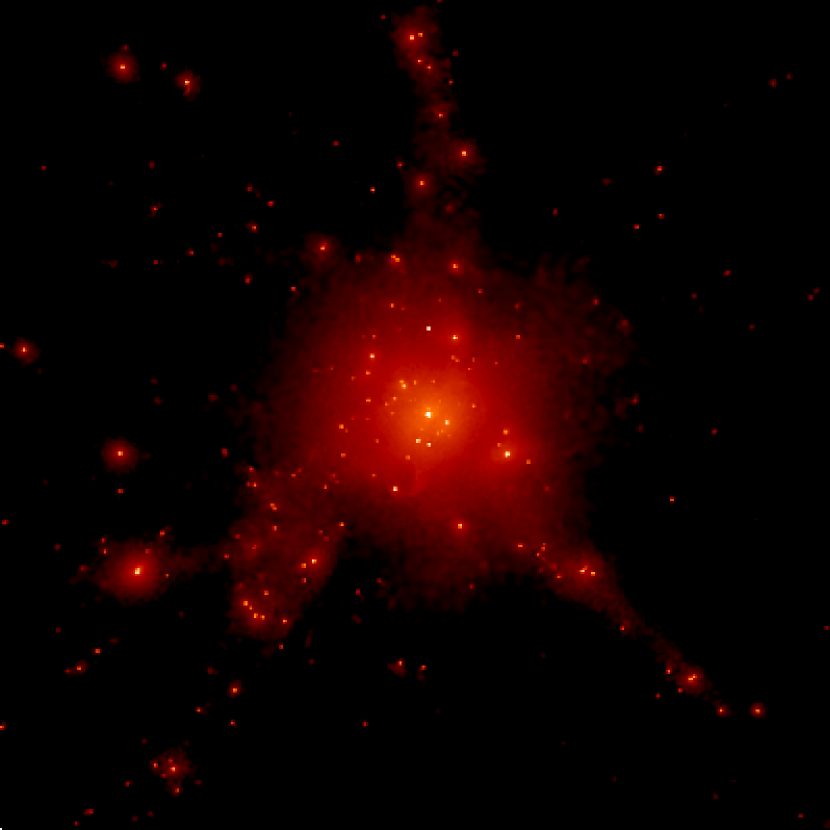
Figure 1: The projected gas density distribution in the simulation at $z=0$. The region shown is a cube of $15h^{-1}$Mpc on a side.

Figure 2 shows the distribution of gas in the thermodynamic phase plane. The cold, dense gas particles appear clearly as a narrow tail in the plot, whereas the shock-heated gas and the adiabatically cooled, unshocked gas appear in the upper and in the lower left portions, respectively. The rectangular box approximately separates out the gas particles in the ‘galaxy’ phase. In practice we identify galaxies by linking the cold gas particles using the standard FOF technique with a small linking length. We describe our galaxy identification in the next section.

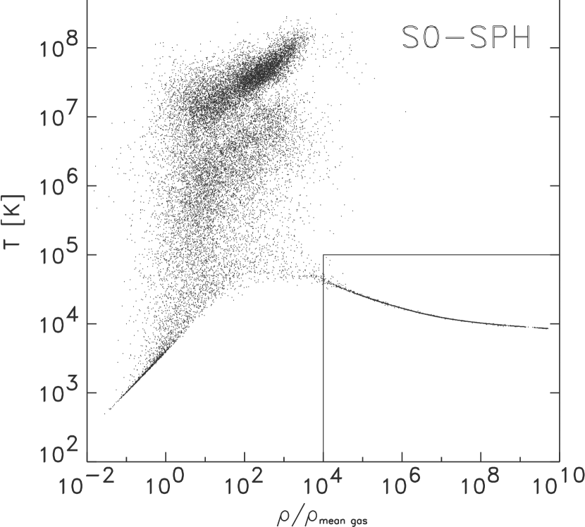
Figure 2: The distribution of gas in the density-temperature plane at $z=0$. Densities are normalised to the mean gas density.

3 Cold and hot gas in dark matter halos

In this section we show the distribution and the properties of gas in the dark halos in the simulations. We locate the dark halos by running a FOF group finder with linking parameter $b=0.164$. We assigned virial radii and virial masses to the dark halos in the manner described above. We found 833 dark halos with virial mass larger than $10^{11}h^{-1}M_{\odot}$ at the present epoch.

3.1 Gas mass fraction

In Figure 3 we plot the total gas mass and cold gas fraction against the host halo mass in the ‘entropy’ version of the S0-SPH simulation. Gas quantities are calculated within a sphere of radius $R_{\rm vir}$. We define the cold gas fraction as the total mass of all the cold ($T<100,000$ K) gas divided by the total gas mass within the halo. Three sets of plots for the outputs at z=0, 1, and 2, are shown in Figure 3. In the top panels the solid line indicates the global mean baryon fraction in the simulation, $f_{\rm b}$=0.15. A tight correlation is seen, showing that the baryon fractions of the halos are very close to the universal baryon fraction. At mass scales larger than $10^{12}h^{-1}M_{\odot}$ (corresponding about 80 dark matter particles), the scatter is very small. At early times, there is a clear tendency for the gas fraction to lie slightly above the global fraction. This is a consequence of the rapid loss of pressure support behind the accretion shock when cooling is efficient.

The bottom panels in Figure 3 show that the cold gas fraction is a decreasing function of halo mass and shows relatively little scatter above halo masses of $10^{12}h^{-1}M_{\odot}$. In this regime the cold gas mass fraction at given halo mass becomes progressively lower at lower redshift. This behaviour is expected as a result of the decrease in cooling efficiency at lower redshift produced by the lower gas density within halos. It confirms that the new SPH implementation substantially reduces over-cooling of gas. In the simulation carried out with the conventional SPH implementation, we found the opposite behaviour; the cold gas mass fraction gets progressively higher at lower redshift. This (mis-)behaviour agrees with the experiments of Springel & Hernquist (2001) who showed that an SPH formulation with geometric symmetrisation can substantially overestimate the cooling rates in the centres of halos, leading to the accumulation of too much cold gas. The cold gas fractions are near 80% for most halos at $z=0$ in our simulation using this scheme, much larger than the values plotted in Figure 3. Even for the main cluster halo itself, the cold gas fraction is overestimated by a factor of 2.

Although the small scatter and the systematic trends in cold gas fraction seen above a halo mass of $10^{12}h^{-1}M_{\odot}$ in Figure 3 are in good agreement with simple semi-analytic models (e.g. White & Frenk 1991 and Section 5 below), the increase in scatter below $10^{12}h^{-1}M_{\odot}$ is unexpected. This is a consequence of resolution problems in the SPH simulation. When a halo contains relatively few gas particles, the smoothing inherent in the SPH technique reduces the estimated gas density to the point where the cooling rate is seriously underestimated. As is clearly visible in the figure, the effect is worse at $z=0$ than at higher redshifts because of the lower mean cooling rates at later times. We will return to the effective resolution limit implied by this problem in Section 5.

At redshift $z=1$ and particularly at $z=2$, another interesting effect is visible at small masses in Figure 3. As the typical cold gas fraction approaches 100% the cold gas mass within halos rises systematically above the nominal maximum given by the halo mass times the global baryon fraction. At the lowest masses this effect is about a factor of two. Although this may, in part, be due to SPH artifacts in the strong cooling and small particle number limit, much of the effect is undoubtedly real. When cooling is efficient shocks are unable to raise infalling gas to the virial temperature of a halo, no significant hot gas atmosphere is formed and the accretion shock moves in close to the halo centre. The total gas mass within the nominal halo radius then increases since pressure effects no longer impede infall at larger radii. We note in passing that this effect is not correctly included in the semi-analytic model we discuss below, which assumes that the maximum mass which can cool in any halo is $f_{\rm baryon}M_{\rm halo}$.

We close this section by mentioning a different cooling problem. As noted above, it has been known for more than twenty years that feedback of some kind is needed in hierarchical cosmogonies to prevent excessive cooling and star-formation at early times. Katz & White (1993; see also Evrard, Summers & Davis 1995; Suginohara & Ostriker 1998) demonstrated that such over-cooling occurs in hydrodynamic simulations of CDM universes provided these are able to resolve the relevant early phases of evolution. Subsequent work by Lewis et al. (2000) and Pearce et al. (2001) confirmed that the cold gas fraction indeed increases with increasing resolution. In our simulation, the cold gas fraction of the main cluster is about 23% at the present epoch (see the rightmost point in Figure 3). Although this value is substantially smaller than the 55% which we found in the simulation with the conventional SPH implementation, it still appears too high to be compatible with observational constraints on the fraction of baryons locked up in stars in rich clusters (Balogh et al. 2001). This again confirms that efficient feedback mechanisms are required to regulate cooling and star formation in realistic models. Nevertheless, since our aim is to compare the treatment of gas cooling in SPH and SA simulations, this ‘cooling catastrophe’ is not directly relevant to our analysis.

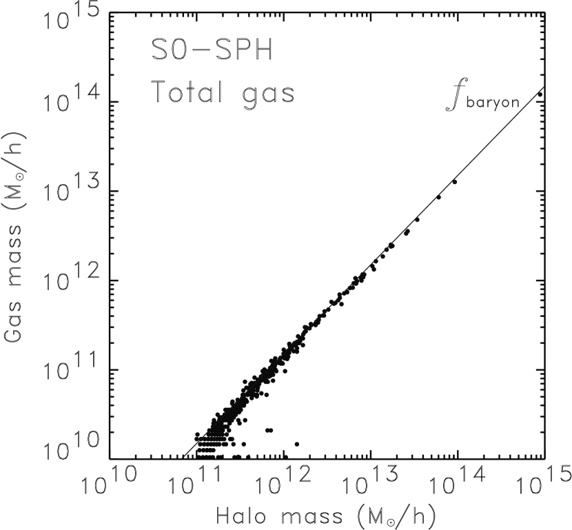
Figure 3: We plot the total gas mass (top) and the cold gas fraction (bottom) against halo mass at $z=0$. The solid line in the top panel indicates the global baryon fraction. If a dark halo is empty of cold gas, we assign a very small value instead of zero to the corresponding fraction, so that those halos also appear in the figure.

Figure 3: -continued. $z=1$.

Figure 3: -continued. $z=2$.

3.2 ‘Galaxies’ in the SPH simulations

In our two versions of the S0-SPH simulation, we define cold, dense clumps of gas as ‘galaxies’. We locate these objects by running a FOF group finder over the gas particles with a very small linking parameter, $b=0.016$. We note that the choice of linking parameter is not particularly critical; adopting a slightly smaller or larger value makes only a minor difference to the number of galaxies and their masses. We also checked that for our chosen value most cold, dense particles in the more massive halos are linked into galaxies, and multiple galaxies within a single halo are successfully separated into discrete objects. In the following we require a clump to contain ten or more gas particles to be considered as a galaxy, corresponding to a minimum mass of $2.1\times 10^{10}h^{-1}M_{\odot}$. We refer to such objects as SPH galaxies, in contrast to the SA galaxies defined using the semi-analytic model. The mass of an SPH galaxy is simply the mass of its grouped particles. We note that it may not be appropriate to regard $N_{\rm min}$ SPH particles as a distinct group, where $N_{\rm min}\leq N_{\rm NGB}$, because of the SPH smoothing with $N_{\rm NGB}$ particles. Nevertheless we include such small groups in our SPH galaxy catalogue, because, at early epochs, many of them are progenitor galaxies with which we can keep track of the formation history in detail. We give an extensive discussion on the resolution of our SPH simulation in section 5.

4 Semi-analytic simulations of galaxy formation

In the galaxy formation models of KCDW and of SWTK, outputs of high resolution N-body simulations are used to define populations of dark halos and to follow their formation and evolution. Although the merging of halos is followed explicitly by these simulations (as is also the evolution of halo substructure in SWTK), all aspects of the evolution of the baryonic component are included using simple, physically motivated, recipes taken from earlier semi-analytic models. In this paper we follow the procedures of KCDW, simplified to exclude processes other than gas cooling and ‘galaxy’ merging. This eliminates the free parameters normally adjusted in SA models, since these are associated with star formation and feedback. The standard cooling model contains no free parameters (see below) and the merger model of KCDW implies merger rates in good agreement with those seen in simulations where merging can be followed explicitly (SWKT).

For each dark halo in each simulation output, we assign the following related halo properties: the virial radius $R_{\rm vir}$, the virial mass $M_{\rm vir}$, and the circular velocity $V_{\rm vir}^{2}=GM_{\rm vir}/R_{\rm vir}$. These halos are linked to their progenitors in the previous output to build up merger history trees within which the growth of galaxies is followed. Notice that since we use the dark matter distribution from the $N$-body/SPH simulation to set up these trees, there is an exact correspondence between the halos and their merger histories in our SA and SPH simulations. Any differences in the resulting galaxy populations must therefore be produced purely by differences in how gas dynamics, cooling and galaxy merging are handled. We now turn to the assumptions used to model gas cooling.

4.1 Gas cooling

Gas cooling is treated as in White & Frenk (1991). We assume that the gas in a dark halo is shock-heated to the virial temperature and is initially distributed like a singular isothermal sphere with density profile $\rho_{\rm g}\propto r^{-2}$. We define the local cooling time of the gas, $t_{\rm cool}$, as the ratio of the thermal energy density of the gas to the cooling rate per unit volume:

$$t_{\rm cool}(r)=\frac{3}{2}\frac{kT\rho_{\rm g}}{\bar{\mu}m_{\rm p}n_{\rm e}^{2}(r)\Lambda(T,Z)},$$ (1)

where $\bar{\mu}$ is the mean molecular weight, $m_{\rm p}$ is the proton mass, $n_{\rm e}$ is the electron number density, $T$ is the gas temperature, which we approximate with the virial temperature of the halo $T=35.9(V_{\rm vir}/{\rm kms}^{-1})^{2}$ K, and $\Lambda(T,Z)$ is the cooling rate. We employ the tabulated cooling functions of Sutherland & Dopita (1993).

We define a cooling radius $r_{\rm cool}$ such that the cooling time at this radius is equal to the time for which the halo has been able to cool quasi-statically. We approximate this time with the halo’s dynamical time $R_{\rm vir}/V_{\rm vir}$. The cooling rate for the gas within this cooling radius is then given by

$$\frac{{\rm d}M_{\rm cool}}{{\rm d}t}=4\pi\rho_{\rm g}(r_{\rm cool})r^{2}_{\rm cool}\frac{{\rm d}r_{\rm cool}}{{\rm d}t}.$$ (2)

In reality, cooling rates depend strongly on the metallicity of the gas, but for simplicity (and consistency) we use zero metallicity cooling functions in both our SA and our SPH models.

We note that this cooling model is extremely simplified and corresponds quite poorly to the detailed dynamics seen in hydrodynamic simulations of the evolution of galaxy-sized objects in a CDM universe. The good agreement which we find below with the gas accumulation rates in our best SPH simulation is thus quite surprising.

4.2 The stripped-down semi-analytic model

Our SPH simulations do not include star formation or feedback processes. In order to make a direct comparison, we remove these processes also from our semi-analytic simulation. In this stripped-down model, star formation and feedback are switched off, and no cooling cut-off is implemented in massive halos (c.f. KCDW). As in the SPH simulations, galaxies in our stripped-down SA simulation do not possess properties such as luminosity or morphological type. They are defined purely by their mass of cold gas, their positions and velocities, and their formation histories. There are only two populations of galaxies in this model. Each dark halo carries exactly one central galaxy which is identified with the most-bound particle of the halo. Many halos have also one or more satellite galaxies. Satellites are galaxies that were central galaxies in earlier outputs, but whose host halos merged at some time into the larger halo where they now reside. Satellites are identified with the particle to which they were attached when they were last a central galaxy. They are assumed to merge with the central galaxy of their new halo on a dynamical friction timescale (see KCDW). In this implementation, only the central galaxy accretes new gas that cools within the halo; hence the mass of a satellite galaxy stays constant.

5 The resolution of the SA and SPH simulations

In this section we discuss the effective resolution limits of our two simulation techniques. The principal goal of our paper is to compare the predictions of these techniques for the cooling of gas onto protogalaxies, but before this is possible we must establish the range of protogalaxy masses for which the predictions of each technique are independent of the resolution parameters – particle mass, force softening, SPH smoothing, timestep – employed in the corresponding simulation. With this in mind, we define the effective resolution of a simulation to be the minimum galaxy mass for which the simulated galaxy population has identical properties to that in a much higher resolution simulation of the same system carried out with the same technique. Notice that with this definition there is no guarantee that the galaxy populations produced by simulations using our two techniques will agree above the larger of their two resolution limits, although we find below that they do. Notice also that for the physical processes included here – cooling, but no star formation or feedback – there is reason to worry that our definition may fail; as the resolution of a simulation is increased the masses of all galaxies might increase systematically towards their maximal possible values, corresponding to the total baryon content of their individual halos. We find below that a ‘cooling catastrophe’ of this type does not, in fact, occur.

We begin by studying the resolution limit of our SA simulation technique. This is relatively straightforward because SWTK have already carried out a series of higher resolution simulations of the physical system studied here. For their highest resolution model, S4, the mass resolution is about 250 times higher and the spatial resolution about 50 times higher than in our S0-SA simulation. We have run our ‘stripped-down’ SA modelling on SWTK’s S4 simulation to derive a galaxy population which can be compared directly with those of this paper. Figure 4 compares the cumulative mass functions of the two SA simulations. Above a mass of about $1.5\times 10^{10}h^{-1}M_{\odot}$ the agreement is good with the masses of galaxies in the high resolution simulation lying slightly below those of galaxies in S0-SA. At lower mass the mass function of S0-SA shows a clear change in slope. This is easily understood. Our halo merger trees keep track of all halos with 10 or more particles. The maximum mass of a galaxy which could form in an unresolved halo is thus given by the global baryon fraction times the mass of a 9 particle halo. This is $1.9\times 10^{10}h^{-1}M_{\odot}$, slightly larger than the mass at which we see the change in slope. The convergence tests of SWTK indicate similar resolution limits for their full semi-analytic model.

It is important to note the very steep mass functions in Figure 4 which are a consequence of the absence of feedback. The total amount of gas cooled in the SA simulations is a strong function of resolution, rising from 16% in S0-SA to 25% in S4-SA. (We have not attempted to include the effects of an ionizing background in the SA modelling, which would reduce the strength of this effect.) It turns out, however, that the additional gas which cools off in small objects does not reduce the reservoir of diffuse gas enough to substantially affect the masses of the larger objects which form later. Similarly merging is not efficient enough for the increased supply of low-mass merger candidates to cause a substantial increase in the masses of larger systems. Thus, although there is no formal convergence as resolution is increased, the properties of the higher mass galaxy population vary very little.

It is more difficult to study the mass limit for our SPH model, because we cannot carry out a similar convergence test to that we decribed above for the SA models. Our decision to impose a 10 particle lower limit on our SPH ‘galaxies’ clearly imposes a lower bound of $2\times 10^{10}h^{-1}M_{\odot}$ on the resolution limit, but Figure 3 shows that the effective resolution limit is substantially higher. Below a halo mass of about $10^{12}h^{-1}M_{\odot}$ many halos contain substantially less cold gas than expected and some contain none at all. This is a consequence of the smoothing associated with SPH density estimates which leads to an underestimate of the cooling in systems where the number of gas particles is comparable to that required within the SPH smoothing kernel. We plot the $z=0$ cumulative galaxy mass function for the ‘entropy’ version of our S0-SPH simulation in Figure 4. Above $1.5\times 10^{11}h^{-1}M_{\odot}$ this function agrees well with that of our two SA simulations, except for a slight shift to higher mass. Below $1.5\times 10^{11}h^{-1}M_{\odot}$ the mass function has a clear change in slope. We take this mass scale as a conservative estimate for the mass resolution of our SPH simulation. This effective resolution limit in our S0-SPH simulation is about an order of magnitude larger than the corresponding limit for our S0-SA simulation. In light of this a robust comparison of SA- and SPH-galaxies can only be made at masses larger than about $10^{11}h^{-1}M_{\odot}$.

Figure 4: The cumulative mass functions of the ‘galaxies’ (i.e. the cold clumps of dense gas) in the semi-analytic and SPH simulations. We indicate the effective mass resolutions discussed in the text using vertical bars. The galaxy mass function for the S4-cluster (the highest resolution simulation of the same cluster in Springel et al. 2001b) is plotted for comparison. The mass resolution of this simulation is 250 times better than that of the SA simulation studied in this paper.

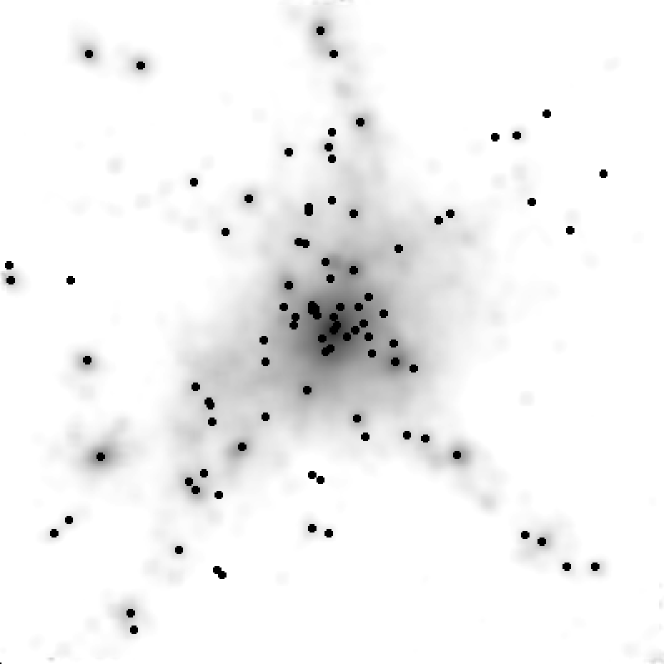
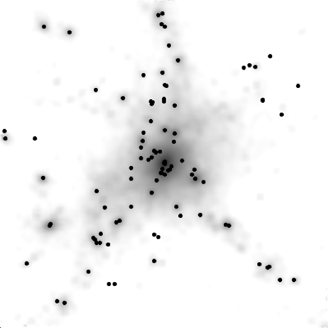
Figure 5: Distribution of SA-galaxies (top) and SPH-galaxies (bottom) at $z=0$. Only galaxies with mass larger than $6\times 10^{10}h^{-1}M_{\odot}$ are plotted in the figures. The grey scale shows the projected density (gas and dark matter) distribution.

6 Object-by-object comparison

We now turn to a direct comparison of the properties of the individual objects which form in our SA and SPH simulations. The dark matter distributions of the two simulations are identical at all times, by construction, and as a result it is possible to identify individual galaxies in the two models almost without ambiguity. We begin by comparing the masses of the central galaxies. Every halo with at least 10 particles is automatically assigned a central galaxy in our semi-analytic model (see Section 4.2) whereas defining the central galaxy in the SPH simulation is less clear. For simplicity, we define the most massive SPH-galaxy within a halo to be its central galaxy, and we tag other galaxies as satellites. Note that this definition corresponds closely to that used in the SA model for halos with multiple galaxies (see KCDW).

In Figure 5 we compare the distributions of SA- and SPH-galaxies more massive than $6\times 10^{10}h^{-1}M_{\odot}$ in a cubic region, 15$h^{-1}$Mpc on a side, centred on our cluster. The two distributions are very similar, and an almost one-to-one correspondence can be found. Most of these galaxies are the central galaxies of their dark matter halos except in the main cluster itself where there are many satellites. Thus the galaxy distribution largely reflects that of the centres of the massive halos. Most differences arise when galaxies lie on opposite sides of our mass threshold in the two samples.

In Figure 6 we plot SA mass against SPH mass for the central galaxies of all halos with 10 or more dark matter particles. Halos with no SPH-galaxy are shown on the left of this diagram at an arbitrary SPH mass. Above our SPH effective resolution limit ($\sim 10^{11}h^{-1}M_{\odot}$) the central galaxy masses predicted by our two techniques agree extremely well over more than two orders of magnitude in mass. Below this limit the masses of the SPH-galaxies are systematically low and many halos contain no SPH-galaxy even though the corresponding SA-galaxy mass is well above $2\times 10^{10}h^{-1}M_{\odot}$, the limit imposed by our requirement that an SPH-galaxy contain at least 10 particles. We emphasize that the agreement above $10^{11}h^{-1}M_{\odot}$ limit is remarkable considering the crudity of the cooling model used in the SA treatment and the fact that our two implementations of SPH lead to galaxy masses differing systematically by a factor of two. (In this section we only show results from the ‘entropy’ implementation.)

It is also interesting to see the evolution of the masses in two models. In Figure 7 we compare the masses of the three most massive galaxies at $z=0$ and their progenitors at earlier epochs. It is clearly seen that even the time evolution is remarkably similar in the two models. Small deviations from the perfect linear relation at output instants are due to time offset of satellite merging onto the central galaxy, because of the simplified prescription of satellite merging in our SA model.

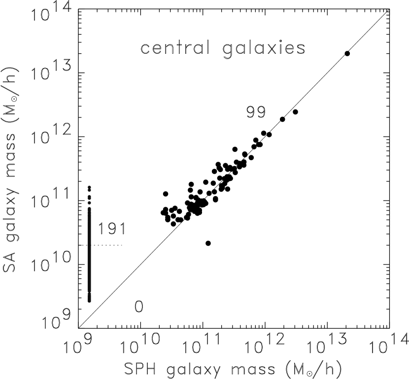
Figure 6: The SA-galaxy mass is plotted against the SPH-galaxy mass for central galaxies (top) and for satellite galaxies (bottom). If a dark halo hosts a SA(SPH) central galaxy but no SPH(SA) galaxy, we assign a very small value instead of zero as the corresponding SPH(SA) galaxy mass. These galaxies then also appear in the figure. The number of such galaxies is given beside the points at very low mass. For satellite galaxies, we plot the satellite - satellite matching cases as filled circles. The numbers in parentheses are the number of SPH-satellites which are matched to SA-centrals (right lower corner) and of SA-satellites which are matched to SPH-centrals (left upper corner). These galaxies are plotted as open circles.

Figure 6: -continued. $z=1$.

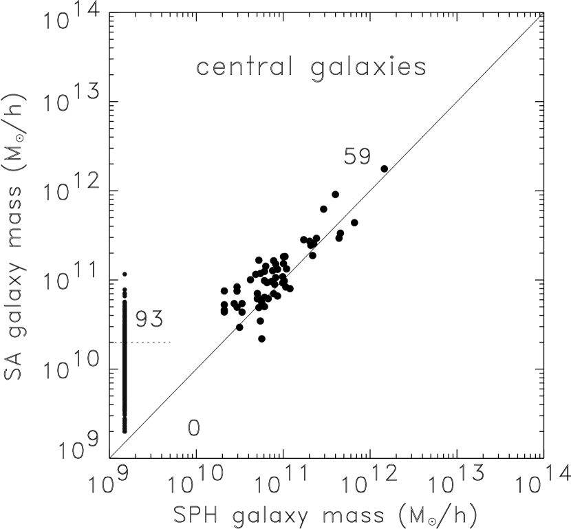
Figure 6: -continued. $z=2$.

A similar comparison for satellite galaxy masses is shown in the bottom panels in Figure 6. In this case matching SA- and SPH-galaxies is much more complicated than for central galaxies. Once an object becomes a satellite its position will not be the same in the two kinds of simulation, and indeed it may merge with the central galaxy in one of the simulations but not in the other. We use the histories of the satellite galaxies in the two simulations in order to carry out this matching. Given a satellite galaxy identified in an output of the semi-analytic simulation, say at redshift $z_{1}$, we track it back through earlier outputs until we find the time when it was last a central galaxy. Let us denote this time $z_{2}$. (Recall that, in our semi-analytic scheme every satellite galaxy was a central galaxy at some earlier time.) We then search in the SPH simulation at $z_{2}$ and identify the SA progenitor of our satellite with the most massive SPH galaxy in its halo. In some cases the halo may contain no SPH galaxy and we then consider our original SA satellite to be unmatched. Otherwise we locate the particles of the matched SPH galaxy in the SPH simulation at $z_{1}$ and consider the SPH galaxy which contains the majority of them to be the counterpart of the original SA satellite. This counterpart may be an SPH satellite, the SPH central galaxy, or (rarely) an ‘orphan’ galaxy outside any halo. Occasionally it can fall below the 10 particle threshold to be considered a bona fide SPH galaxy and we then again consider the original SA satellite to be unmatched.

We also carry out the reverse procedure. Starting from an SPH satellite at $z_{1}$, we trace back its progenitors (defined at each time to be the SPH galaxy which donates the largest number of particles to the galaxy at the subsequent output) until we find one which was the most massive SPH galaxy in its halo. This one we then identify with the SA central galaxy of the same halo. We take particular care to investigate SPH satellite galaxies which appear to have no progenitors. In each output, some new SPH galaxies appear for the first time as satellites; in the previous output, their member particles are already cold and are just condensing at the center of a halo. Due to discrete sampling of the output times, there is always a slight offset between the true formation epoch of SPH galaxies and the time when they are first identified. Their host halo can merge with a larger system during this time. To take this into account, we tag the central SA galaxy in any halo that hosts such a forming SPH galaxy as its counterpart, because it is clear that such pairs indeed correspond closely. In this way we can partially compensate for incompleteness in our SPH–SA galaxy matching procedure. The $z_{1}$ descendent of the matched $z_{2}$ SA galaxy is identified as the counterpart of the original SPH satellite. Again, this counterpart may be a satellite, a central galaxy, or (rarely) an ‘orphan’. We find 40 out of 84 SPH satellite galaxies at $z=0$ matched to SA satellites. Another 34 are matched to SA central galaxies. The remaining 10 are unmatched, mostly because they were formed under peculiar conditions in large halos without being at the center of the halos. It is likely that many are associated with subhalos within the large halo, but our simulation does not have adequate resolution to trace their formation in detail.

There are 8 SA satellites which are matched to SPH central galaxies, and 74 SA satellites more massive than $2\times 10^{10}h^{-1}M_{\odot}$ which are unmatched. A few of the latter may, in fact, correspond to unmatched SPH satellites; most correspond to systems in which the SPH gas did not cool. The small number of SA satellites matched to SPH centrals in comparison with the number of SPH satellites matched to SA centrals is a consequence of the lower effective resolution of the SPH simulation. We have checked that the merging rate, estimated as the fraction of all satellites which merge between two output times, is actually very similar in the two simulations.

Figure 7: We plot the mass evolution for the 3 most massive galaxies. Dotted lines show their mass trajectories, and symbols highlight the masses at 4 output redshifts; z=0 (diamond), z=1 (circle), z=2 (square), and z=4 (triangle). Lines and symbols for the 3 galaxies are offset vertically by an order of magnitude each.

Satellite-satellite matches are plotted as filled circles in Figure 6, whereas SA satellite – SPH central and SA central – SPH satellite matches are plotted as open circles. Unmatched satellites are plotted at an arbitrary small value of the ‘missing’ mass and so appear along the left and bottom edges of the diagrams. The numbers of matches of each type are listed explicitly. The number given for the unmatched SA satellites corresponds to objects with masses above $2\times 10^{10}h^{-1}M_{\odot}$, the minimum mass for an SPH galaxy.

For satellite–satellite matches the correspondence between the masses found using our two techniques is still reasonably good although with considerably more scatter than was the case for central galaxies. There is a tendency for the SPH masses to be larger than the SA masses suggesting that gas is continuing to cool onto the galaxies after the time when they are last identified as central objects. It should be noted that a group of points appearing in the lower portion of the plot, indicating SPH satellites matched to small mass SA satellites, are mostly those which are matched by our particular treatment for forming SPH galaxies, as explained above. In such cases, the halos hosting the forming galaxies merge into larger halos before the next output. Their central SA galaxies then become satellites, and their masses stay constant, whereas the SPH galaxies grow in mass continually until (and even after) they actually become satellites. Unsurprisingly, for the satellite – central galaxy matches the central galaxy mass is almost always substantially larger than the satellite galaxy mass, regardless of which is SPH and which SA. It is noticeable that as one moves to higher redshift, the number of unmatched SPH satellites increases substantially relative to the number of unmatched SA satellites. This is probably a reflection of the limited time resolution of our merger trees. At early times structure is building up very rapidly and cooling is efficient. The spacing between our outputs may then be too large to resolve the formation and merging of significant numbers of halos. These can form an SPH galaxy and turn it into a satellite between two levels of our numerical merger tree. In such cases the SA scheme will miss the satellite altogether. This highlights a different resolution issue from those discussed above. The SA scheme must store data sufficiently frequently that no significant stages of halo formation are missed.

In general, we conclude from the overall level of agreement seen for individual central and satellite galaxies that the standard recipe of gas cooling in the semi-analytic model gives an adequate description of the cooling process in the SPH model.

7 Summary and discussion

We have studied the cooling and condensation of gas onto protogalaxies using two very different treatments of the gas physics within the same simulation of dark matter evolution. One treatment uses schematic recipes taken from semi-analytic galaxy formation models, while the other tries to follow the hydrodynamics ‘correctly’ and in detail using an SPH approach. We have also tested two different implementations of the SPH equations, confirming Springel & Hernquist’s (2001) conclusion that the outcome of a simulation can depend sensitively on such details. In our case the two SPH approaches lead to ‘galaxy’ masses which differ by a factor of 2, even for objects which are apparently well resolved. We believe the energy and entropy conserving implementation of Springel & Hernquist (2001) to be the most reliable and have concentrated on it when comparing SPH results to those of the semi-analytic simulation.

We have characterised the effective resolution limit of simulations using each of our gas modelling techniques by the lower limit for which the simulated galaxy mass function agrees with that of a much higher resolution simulation carried out using the same technique. For the SA modelling this galaxy mass limit is just below the total baryon content of the least massive halo included in construction of the merger trees (10 particles in the models used here). For the SPH modelling the effective resolution limit is significantly higher, particularly at low redshifts when cooling times exceed the age of the Universe in most resolved halos. For the simulations studied here the SPH mass resolution limit at $z=0$ is roughly an order of magnitude larger than the SA limit, corresponding to a galaxy of about 75 SPH particles.

Above the resolution limit of both techniques (i.e. for galaxy masses above $\sim 10^{11}h^{-1}M_{\odot}$) the $z=0$ galaxy populations found by the two methods correspond remarkably well on an object-by object basis. The agreement is particularly good for the most massive galaxies in each halo (the ‘central’ galaxies). For satellite galaxies the agreement is still reasonably good for objects which match between the two types of simulation, but two significant types of discrepancy occur. One concerns objects which merge with the central galaxy in one of the simulations but not in the other. This is inevitable given the crudity of the recipe used to determine merging probabilities in the SA model. The difficulty can be avoided, at least for the more massive galaxies, with $N$-body simulations of high enough resolution. The dark matter substructures associated with satellite galaxies can then be tracked explicitly and no SA recipe is needed to follow their merging (see SWTK).

A more interesting discrepancy is the significant number of SPH satellites, which are unmatched in the SA simulation. Some of these may reflect insufficient time resolution in the simulation outputs from which the SA merger trees are constructed; halos may collapse, form galaxies, and merge into a larger halo between two of the stored outputs. Other unmatched SPH satellites may reflect more fundamental failures of the SA scheme. A forming dark halo may be sufficiently irregular to cool gas onto two galaxies rather than one, or cooling shocks associated with large-scale structure may fragment to make galaxies without any associated halo. The number of unmatched SPH satellites is clearly greater at early times than at $z=0$, suggesting that the process producing these objects is more effective when cooling times are short and structure growth is more rapid. This issue clearly warrants further investigation. Although the unmatched SPH satellites are a small population above the effective resolution limit of the SPH simulation, they probably signal a real failure of the SA scheme.

It is instructive to compare the computational efficiency of our two schemes. The comparison of this paper is based on implementing each of the schemes on top of a dark matter simulation with given $N$. For the SA scheme the overhead in post-processing, although non-negligible, is not dominant. Thus the computational cost is essentially that of running the high resolution cosmological $N$-body simulation. The SPH scheme requires an additional $N$ SPH particles, the force calculation for the SPH particles is considerably more complex than for the dark matter particles, and substantially shorter timesteps are needed to get convergent results in an SPH simulation with cooling than in the corresponding pure dark matter simulation. As a result, somewhat more than twice the memory and roughly an order of magnitude more CPU time are needed to carry out the SPH simulation than the corresponding pure $N$-body simulation. (The actual CPU factor for the simulations of this paper was about 20, but in neither case were the simulation parameters optimally chosen for the particular configuration treated.) We have seen, however, that the effective galaxy mass resolution of the SPH simulation is roughly an order of magnitude worse than that of SA simulation. Thus an SPH simulation with ten times as many particles would be needed to get a galaxy population with the same effective mass resolution as the SA simulation. This would require 20 times as much memory and more than two orders of magnitude more CPU time than the SA simulation.

In practice these considerations imply that simulations can be carried out using the SA technique which are far beyond the current capabilities of the SPH technique. For example, the S4 cluster simulation of SWTK has 250 times better mass resolution than the SA simulation of this paper and so of order 2000 times better resolution than our SPH simulation. It will be a long time before we can consider an SPH cluster/galaxy formation simulation with 2000 times more particles than the one analysed above. A further advantage of the SA technique is that the assumptions about uncertain aspects of the galaxy formation modelling (e.g. the mode and efficiency of star-formation or feedback) can be changed without any need to rerun the simulation. An example of this was shown in Figure 4, where the predictions of the high resolution S4 simulation in the absence of star-formation and feedback could be calculated from the stored simulation output. Thus for simulations concentrating on the global properties of the galaxy population and their dependence on the ‘subgrid’ physics (star formation, feedback, etc.) the SA technique is clearly the method of choice.

On the other hand, it is obvious that the SA technique can only be as good as the recipes on which it is based. Our work has shown that the standard gas cooling prescription works surprisingly well, but has also uncovered some apparent discrepancies. Discrepancies of this kind can only be studied and understood through comparison with simulations (or analytic models) which attempt to follow the relevant physics from first principles. Such models or simulations are also needed, of course, to design the SA recipes in the first place. In addition there are many aspects of galaxy formation where SA modelling can only give crude indications. Confirmation through direct simulation is then indispensable. Examples include the internal structure of galaxies, the structure of the intergalactic medium, and the comparison of both of these with the wealth of available data. Galaxy formation and its interaction with the environment is a complex and highly nonlinear process involving many different aspects of astrophysics. Gaining some understanding will require concerted use of all the observational and theoretical weapons at our disposal. SA and SPH simulation techniques will both remain major parts of our theoretical arsenal.

We thank Simone Marri and Hugues Mathis for helpful comments.

References

- [1] Balogh, M. L., Pearce, F. R., Bower, R. G., Baugh, C. M., & Kay, S. T., 2001, astro-ph/0104041
- [2] Benson, A. J., Cole, S., Frenk, C. S., Baugh, C. M., & Lacey, C. G., 2000, MNRAS, 311, 793
- [3] Benson, A. J., Pearce, F. R., Frenk, C. S., Baugh, C. M., & Jenkins, A., 2001, MNRAS, 320, 261
- [4] Cole, S., Aragon-Salamanca, A., Frenk, C. S., Navarro, J., & Zepf, S. E., 1994, MNRAS, 271, 781
- [5] Cole, S., Lacey, C. G., Baugh, C. M., Frenk, C. S., 2000, MNRAS, 319, 168
- [6] Davè, R. E., Hernquist, L., Katz, N., & Weinberg, D. H., 1999, ApJ, 511, 521
- [7] Evrard, A. E., Summers F. J. & Davis, M., 1994, ApJ, 422, 11
- [8] Kauffmann, G., White, S. D. M., & Guiderdoni, B., 1993, MNRAS, 264, 201
- [9] Kauffmann, G., Nusser, A. & Steinmetz, M., 1997, MNRAS, 286, 795
- [10] Kauffmann, G., Colberg, J. M., Diaferio, A., & White, S. D. M., 1999, MNRAS, 303, 188 (KCDW)
- [11] Katz, N. & White, S. D. M., 1993, ApJ, 412, 455
- [12] Katz, N., Weinberg, D. H., & Hernquist, L., 1996, ApJ, 505, 19
- [13] Lacey, C. & Silk, J., 1991, ApJ, 381, 14
- [14] Lewis, G. F. et al. 2000, ApJ, 536, 623
- [15] Pearce, F. R., Jenkins, A., Frenk, C. S., Colberg, J. M., White, S. D. M., Thomas, P. A., Couchman, H. M. P., Peacock, J. A., Efstathiou, G. (The Virgo Consortium), 1999, ApJ, 521, L99
- [16] Somerville, R. S. & Primack, J. R., 1999, MNRAS, 310, 1087
- [17] Springel, V., & Hernquist, L., 2001, astro-ph/0111016
- [18] Springel, V., Yoshida, N., & White, S. D. M., 2001a, New Astronomy, 6, 79
- [19] Springel, V., White, S. D. M., Tormen, G., & Kauffmann, G., 2001b, MNRAS, 328, 726 (SWTK)
- [20] Suginohara, T. & Ostriker, J. P., 1998, ApJ, 507, 16
- [21] Sutherland, R. S. & Dopita, M. A., 1993, ApJS, 888, 253
- [22] Weinberg, D. H., Hernquist, L., & Katz, N., 1997, ApJ, 477, 8
- [23] White, S. D. M. & Rees, M. J., 1978, MNRAS, 183, 341
- [24] White, S. D. M., 1996, in Schaeffer, R., Silk, J., Zinn-Justin, J., eds. Cosmology and Large Scale Structure, Les Houches Lectures
- [25] White, S. D. M., & Frenk, C. S., 1991, ApJ, 379, 52
- [26] White, M., Hernquist, L., & Springel, V. 2001, ApJ, 550, 129
- [27] Yoshida, N., Springel, V., White, S. D. M., & Tormen, G, 2000a, ApJ, 535, L103
- [28] Yoshida, N., Springel, V., White, S. D. M., & Tormen, G, 2000b, ApJ, 544, L87
- [29] Yoshida, N., 2001 PhD thesis, Ludwig-Maximilian University, Munich.