Heavy Nuclei Enrichment of the Galactic Cosmic Rays at High Energy: Astrophysical Interpretation

Abstract

A substantial increase of the mean logarithmic mass $\langle\ln A\rangle$ of galactic cosmic rays vs energy has been observed . We study three effects that could explain this trend i) different source spectra for protons and heavy nuclei ii) a selective nuclear destruction in flight of heavies iii) a gradient of the source number and chemical composition in the galactic disk. We take advantage of the diffusive cosmic ray propagation model developed at LAPTH to study specifically the geometrical aspects of the propagation and extend it to high energy. Using a simple modeling of the spectral knee around $10^{15}$ eV, a bump in $\langle\ln A\rangle$ appears. This feature is smoother when the spectral index of protons is steeper than Fe’s. We analyze the effects of the rigidity dependence of the diffusion coefficient and the scale height of the confinement halo and we show that $\langle\ln A\rangle$ is most sensitive to the first parameter. Pure geometrical effects are less determining than the diffusion coefficient spectral index. Subsequently, we conclude that the physics of cosmic ray confinement is the essential cause of the heavy nuclei enrichment until $\sim 10^{15}$ eV.

, , ,

Introduction

Recent measurements of the cosmic ray average logarithmic mass and all-particle spectrum around $10^{15}$ eV [1, 2] give new clues to understand the origin of the cosmic rays and in particular the puzzle of the knee in the energy spectrum. Analysis of such data in a coherent theoretical framework is a rough task, and even if much progress has been done both in theoretical and experimental sides, none of the models proposed so far to solve this problem has been unanimously accepted. The highest energy particles are almost certainly extragalactic. A similar origin is not excluded near the knee, but it is difficult to account for the observed continuity of the spectrum in this region [3]. As a consequence, the intermediate region between $10^{15}$ and $10^{19}$ eV should be analysed in terms of the same physical mechanisms than lower energy particles.

There are at least three explanations for the knee: (i) a change in propagation parameters (diffusive regime), (ii) a change in the source regime, (iii) a change related to the properties of high energy interactions in the atmosphere or a subtle combination of all three. As Schatz [4] emphasized recently, the fine structure of the knee in all-particle spectra provided by extensive air showers can help to discriminate between these solutions. Furthermore, recent data from collider seem to show no drastic departure from cross sections predictions in the range 100 – 1000 TeV [1]. Anyway, this paper will only concentrate on astrophysical aspects.

More information can be obtained by measuring $\langle\ln A\rangle$. All-particle spectrum and $\langle\ln A\rangle$ are given by linear combination of the individual fluxes with different weights;

$$\Phi^{\rm all}\equiv\sum_{j}\Phi_{j}$$

and

$$\langle\ln A\rangle\equiv\frac{\sum_{j}\ln A_{j}\Phi_{j}}{\sum_{j}\Phi_{j}}\;.$$

Therefore they provide different information of these fluxes. Obviously, these weighted quantities are not very useful at “low energy” where all nuclei are well resolved in satellite or balloon experiments (for a compilation of data, see [5]). Experimental difficulties arise around and above the knee: fluxes are very low ($\sim$ m^-2 sr^-1 yr^-1) and large ground array detectors are needed to collect unresolved events with a good statistic. Incidently, the all-particle spectrum can be extracted via shower parameters (e.g. core position, direction,…) and an estimation of the average logarithmic mass is also possible through various methods (e.g [2, 6, 7] and in particular [8]). A new experimental technique has been recently proposed, which can potentially yield excellent charge resolution measurements near and above the knee [9]. But at the present time, even if a few solutions exist to infer the composition [10, 11], all-particle flux, mean logarithmic mass and sometimes proton and helium spectra [12] are grossly the only available observables near and above the knee (for a detailed revue, see [13]).

The paper is organized as follows: (i) features of primary species propagated in diffusion model are reminded; (ii) simple models are used to explore the behaviour of $\langle\ln A\rangle$ considering separately the effect of three parameters (source spectra, propagation, geometrical aspects); (iii) the results of these simplified models are analysed; (iv) using a more realistic simulation, the three parameters are discussed in details, and (v) all these parameters are included in the propagation model of Maurin et al. [14] and are finally combined to analyze the knee problem.

1 Basic features of propagation models

For practical reasons, spectra at low energy are almost always displayed in units of kinetic energy per nucleon, because this quantity is conserved in nuclear reactions. This convention has become the rule in the analysis of cosmic ray propagation, e.g. secondary to primary ratio studies. Above PeV energies, fluxes are plotted vs energy per particle because it is the only observable provided by ground observatories. Whereas various primary species present similar spectra when plotted versus kinetic energy per nucleon or rigidity, they behave differently in terms of total energy (compare for example Fig. 5-a of [15] that displays fluxes in units of kinetic energy per nucleon and Fig. 2 of [5] that shows the same fluxes, but in units of total energy); so a combination of all the corresponding spectra into a single quantity (for example the average logarithmic mass) will provide a different dependence in terms of total energy or in terms of rigidity.

1.1 Propagation models above the knee and extrapolation to higher energies

Although cosmic ray properties are well understood up to a few hundreds of GeV/nuc (see the recent review of [16]), it is difficult to harmonize all the observables (i.e. protons, nuclei, e^-, e⁺, $\bar{p}$, $\gamma$ rays; see for instance [17]). In particular, the hypothesis according to which the fluxes measured locally are representative of the fluxes present everywhere in the Galaxy is still debated. At intermediate energies, extension of the usual propagation models has mainly to face the problem that the observed anisotropy is very low. This seems to favor a Kolmogorov spectrum (interstellar turbulence) associated to the rigidity dependence of the diffusion coefficient (see discussion in [18]).

Cosmic ray spectra are affected by the propagation process. Maurin et al. [14] have recently developed a propagation model (see Sec. 4.2 for details) that is in principle valid for a wide energetic range as long as charged nuclei are considered. This is a two zones model (thin gazeous disc – half-height $h=100$ pc – and large diffusive halo $L\sim 3-10$ kpc) where cylindrical symmetry is assumed (radial extension, $R=20$ kpc). The steady–state differential density $N^{j}(E,\vec{r})$ of the nucleus $j$ as a function of energy $E$ and position $(r,z)$ in this model is given by

$${L}_{dif\!f}N_{j}(r,z)+2h\delta(z)\left(q^{j}_{0}Q_{j}(E)q(r)+\sum_{k=1}^{j-1}\Gamma^{kj}N_{k}(r,0)-\Gamma^{j}N_{j}(r,0)\right)$$

$$=2h\delta(z)\frac{\partial}{\partial E}\left\{b^{j}(E)N_{j}(0)-d^{j}(E)\frac{\partial}{\partial E}N_{j}(0)\right\}$$

$${L}_{dif\!f}\equiv-V_{c}\frac{\partial}{\partial z}+K(E)\left(\frac{\partial^{2}}{\partial z^{2}}+\frac{1}{r}\frac{\partial}{\partial r}(r\frac{\partial}{\partial r})\right)$$

The operator ${L}_{dif\!f}$ represents convection ($V_{c}$) plus spatial diffusion ($K(E)=K_{0}\,\beta\times R^{\delta}$) acting in the whole box. All other terms describe processes localized in the thin gazeous disc only: the bracket corresponds to primary source term, secondary spallative production from heavier nuclei, and destruction cross section (radioactive-induced processes have been omitted here). Curly bracket provides all terms leading to energetic redistribution, i.e losses (Coulombian, ionisation and adiabatic expension losses) and gains (reacceleration) described by two effective parameters $b_{j}(E)$ and $d^{j}(E)$ (for all details, see [14]).

In the leaky box model, widely used, all the quantities are spatially averaged. The diffusion-convection term is then replaced by an effective escape term which has the meaning of a residence time $\tau_{esc}$ ($\sim 20$ Myr at a few GeV/nuc) in the confinement volume ($-L_{dif\!f}\leftrightarrow\tau_{esc}^{-1}$). If energy gains and losses are discarded, the leaky box equation reads

$$-\frac{\bar{N}_{j}}{\tau_{esc}}+\left(\bar{q}^{j}_{0}Q_{j}(E)+\sum_{k=1}^{j-1}\Gamma^{kj}\bar{N}_{k}-\Gamma^{j}\bar{N}_{j}\right)=0$$

As an immediate consequence, leaky box models do not allow to take in consideration, for example, a radial dependence of Galactic sources. More generally, any subtle effect related with spatial dependence of any terms of the diffusion-convection equation is automatically swept away.

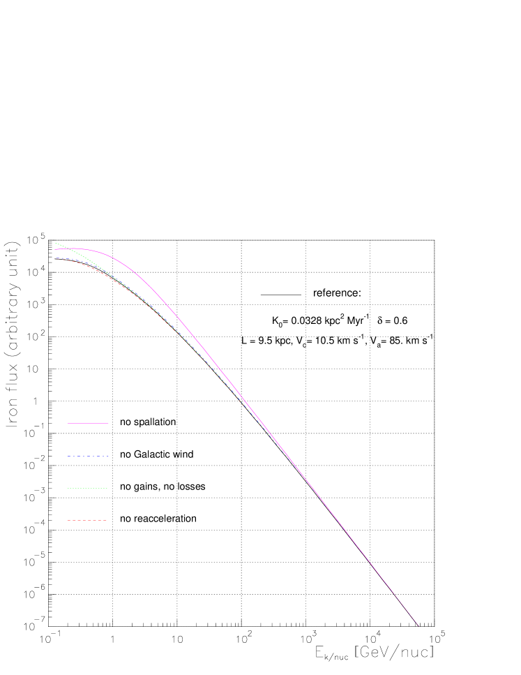
Figure 1: Unnormalized Fe flux for a typical propagation model that reproduces B/C (reference curve); the five parameters (diffusion – normalization $K_{0}$ and slope $\delta$ –, halo size $L$, convection $V_{c}$, reacceleration $V_{a}$) are taken from [14]. Other curves correspond to the same propagation parameters, except one that has been switched off.

Figure  1 displays the iron flux as a function of kinetic energy per nucleon in our diffusion-convection model; this behaviour is standard for all charged nuclei except protons, for which propagation is less sensitive to nuclear reactions. Within realistic propagation models, several parameters affect the primeval power law source spectrum:

• The most spectacular effect is that of inelastic interactions (nuclear destruction). It becomes negligible ($\lesssim$ a few %) between 1 TeV/nuc and 10 TeV/nuc, depending on the species, since the escape time is shorter than the nuclear time.

• The spectrum is also affected by energy losses up to $\sim 100$ GeV/nuc.

• More controversial effects may be present: galactic wind up to 1 TeV/nuc and reacceleration up to some tens of GeV/nuc.

Propagation effects are present up to 10 TeV/nuc. This induces modifications of spectra up of a few hundreds TeV in total energy, at least for heavier nuclei (i.e. Fe) leading in turn to a dependence on energy of the average logarithmic mass till these higher energies, i.e. near the knee ($\sim$ PeV). Since current high energy data are provided in total energy per particle, all results will be given in total energy (denoted $E$) unless stated otherwise.

2 Separation of key ingredients

Solar modulation is ignored because it has almost no effect on fluxes above a few tens of GeV/nuc. Three items (source spectra, propagation and geometrical effects) are pieces of the cosmic ray puzzle. In this section, we introduce simplified models where only two species are considered (e.g. H and Fe) that allow to analyze qualitatively the increase of the mean mass of cosmic rays with energy.

2.1 Source spectrum effect

In the simplest propagation model that one can imagine, pure diffusion is considered and only two ingredients are necessary:

$$Q_{j}(E)=q^{0}_{j}\times\left(\frac{R}{1\mbox{~{}GV}}\right)^{-\alpha_{j}}\mbox{ is the source spectrum,}$$ (1)

$$K(E)=K_{0}\times\left(\frac{R}{1\mbox{~{}GV}}\right)^{\delta}\mbox{ is the diffusion coefficient.}$$ (2)

In the above expressions, $R=p/Z$ is the rigidity, $q^{0}_{j}$ and $\alpha_{j}$ are respectively the source abundance and the spectral index of nucleus $j$, $K_{0}$ is the normalization coefficient of the diffusion coefficient and $\delta$ its slope (both are assumed independent of the species considered). The detected local flux (in arbitrary units) is thus expressed merely as the ratio of sources over the diffusion coefficient (up to a coefficient $v/4\pi\simeq c/4\pi$ for all nuclei):

$$\Phi_{j}(E)=Q_{j}(E)/K(E).$$ (3)

This model can be viewed as the high energy limit of all diffusion models. This limit is also that of a locally equivalent leaky box model, where once emitted, the nucleus can escape from the confinement box with a probability which is related very simply to $K(E)$ – see for example [14] and references therein.

2.1.1 $\langle\ln A\rangle$ for the two nuclear component model

In a two nuclei model, the evaluation of the Fe/p ratio and the average logarithmic mass number – “average mass” for short – is straightforward. At a given energy, the rigidities of two charged nuclei are different. Indeed, the term $K(E)$ can’t be simply factorized, and some residual multiplicative constant depending on $\delta$ appears. Using the approximate relation $R=p/Z\simeq E/Z$ (E is the total energy per particle) which is correct beyond a few tens of A GeV, we have

$${\rm Fe}/{\rm p}(E)=\left(\frac{q^{0}_{\rm Fe}}{q^{0}_{\rm p}}\times\frac{Z_{\rm Fe}^{\alpha_{\rm Fe}+\delta}}{Z_{\rm p}^{\alpha_{\rm p}+\delta}}\right)_{100\rm~{}GeV}\times\left(\frac{E}{100{\rm~{}GeV}}\right)^{-\alpha_{\rm Fe}+\alpha_{\rm p}}\>,$$

where the first term corresponds to the relative source abundance Fe/p taken at the energy 100 GeV, which is $\sim 1/20$ (see Fig. 2 of compilation of [5]). Apart from numerical constant, we roughly see that the steeper ${-\alpha_{\rm Fe}+\alpha_{\rm p}}$ effective slope, the greater will be the average mass. To be more precise,

$$\langle\ln A\rangle(E)=\frac{\ln(A_{\rm Fe})}{\left(1+\left[(q^{0}_{\rm p}/q^{0}_{\rm Fe})(Z_{\rm p}^{\alpha_{\rm p}+\delta}/Z_{\rm Fe}^{\alpha_{\rm Fe}+\delta})\right]_{\rm 100~{}GeV}\times(E/100{\rm~{}GeV})^{-\alpha_{\rm p}+\alpha_{\rm Fe}}\right)}$$ (4)

whereas in terms of the all-particle spectrum, the evolution – up to a normalization – can be written as

$$\Phi^{\rm all}\propto E^{-\alpha_{\rm Fe}-\delta}\times\left(1+\left[\frac{q^{0}_{\rm p}Z_{\rm p}^{\alpha_{\rm p}+\delta}}{q^{0}_{\rm Fe}Z_{\rm Fe}^{\alpha_{\rm Fe}+\delta}}\right]_{\rm 100~{}GeV}\times\left(\frac{E}{100{\rm~{}GeV}}\right)^{-\alpha_{\rm p}+\alpha_{\rm Fe}}\right)\;.$$ (5)

We remark that in our simple two species model, $\Phi^{\rm all}\propto E^{-\alpha_{\rm Fe}-\delta}/\langle\ln A\rangle(E)$; the behaviour of all-particles spectrum will be discussed in Sec. 3.

2.1.2 Application to the“wind/ISM” supernova model

Among the various acceleration models, some of them are able to produce various spectra for different nuclei (see Sec. 4.1). The maximal source effect is obviously obtained when $|-\alpha_{\rm p}+\alpha_{\rm Fe}|$ is maximal. For typical values $-\alpha_{\rm p}+\alpha_{\rm Fe}\sim-0.1$ such as those advocated by the wind/ISM supernovae model of Biermann and collaborators [19], and with the above value $\left[(q^{0}_{\rm p}/q^{0}_{\rm Fe})(Z_{\rm p}^{\alpha_{\rm p}+\delta}/Z_{\rm Fe}^{\alpha_{\rm Fe}+\delta})\right]_{\rm 100GeV}\sim 20$, we obtain

$$\langle\ln A\rangle(E={\rm 100\>GeV/\>10\>TeV/\>1\>PeV/\>\infty)}\sim 0.19\>/\>0.30\>/\>0.50\>/\>4.03\\$$ (6)

Indeed, the evolution is expected to be smoother when all cosmic ray nuclei are considered, because the slopes of nuclei heavier than hydrogen are similar (see Sec. 4.1); but this sole effect leads to an evolution of the average mass. Incidently, if $\alpha_{\rm p}=\alpha_{\rm Fe}$, we are left with a constant $\langle\ln A\rangle$ that merely depends on the relative abundances of nuclei. This conclusion holds again when several nuclei are considered.

2.2 Propagation effect: same spectral index

The process of inelastic collisions – which differs from one nucleus to another – has a major impact on propagation (see Fig. 1). To obtain order of magnitude estimates, a simple leaky box description including just destruction cross sections is sufficient. Thus, the propagated flux for a primary species $j$ is:

$$\Phi_{j}(E)=\frac{Q_{j}(E)}{1/\lambda_{esc}(E)+\sigma^{inel}_{j}/{\bar{A}}}=\frac{1}{\bar{A}}\times\frac{Q_{j}(E)}{\sigma_{esc}(E)+\sigma^{inel}_{j}}$$ (7)

Here $\sigma^{inel}_{j}=\sigma^{tot}_{i}-\sigma^{el}_{i}$ is the total inelastic (or reaction) cross section of species $j$, and $\lambda_{esc}(E)$ is the usual escape length of the leaky box in g cm^-2 and $\bar{A}$ is the mean mass of the atoms in the interstellar medium. This can also be rewritten in terms of an effective escape cross section $\sigma_{esc}$ (in cm²) that is related to the usual grammage by a simple factor.

Under the assumption of the same source spectrum (i.e. universal slope $\alpha_{j}=\alpha$ for all species) and since there is no geometry in the leaky box, assuming an escape dependence $\lambda_{esc}(E)=\lambda_{0}\beta R^{-\delta}\simeq\lambda_{0}R^{-\delta}$, i.e $\sigma_{esc}(E)=\sigma_{0}R^{\delta}$ for all nuclei, we get:

$$\langle\ln A\rangle(E)=\ln(A_{\rm Fe})\times\left[\left(1+(q^{0}_{\rm p}/q^{0}_{\rm Fe})\times\left(\frac{Z_{\rm p}}{Z_{\rm Fe}}\right)^{\alpha}\times\frac{(\sigma_{0}(E/Z_{\rm Fe})^{\delta}+\sigma^{inel}_{\rm Fe})}{(\sigma_{0}(E/Z_{\rm p})^{\delta}+\sigma^{inel}_{\rm p})}\right)\right]^{-1}$$ (8)

Contrary to the previous case, the ratio $q^{0}_{\rm p}/q^{0}_{\rm Fe}$ does not depend on energy.

2.2.1 Leaky box results

The typical diffusion coefficient for leaky box models is given for example by [20]

$$\lambda=35.1\beta\>(R/1{\rm~{}GV})^{-0.61}\mbox{~{}g cm}^{-2}$$

which corresponds in the above expression to $\sigma_{0}\sim 47$ mb. We have in this model $\alpha\sim 2.2$, $\sigma^{inel}_{\rm p}\sim 30$ mb (Particle Data Group), $\sigma^{inel}_{\rm Fe}\sim 710$ mb [21]. In order to compare this effect with the precedent, we set $q^{0}_{\rm p}/q^{0}_{\rm Fe}$ to $\sim 25000$ which gives the same $\langle\ln A\rangle$ at 100 GeV as before. Thus,

$$\langle\ln A\rangle(E={\rm 100\>GeV/\>10\>TeV/\>1\>PeV\>/\>\infty)}\sim 0.19\>/\>0.83\>/\>1.05\>/\>1.08$$ (9)

Even near the knee energies, the average mass slightly evolves due to spallations. It is then clear from formula (8) that the evolution of chemical abundances depends on (i) the destruction cross section, (ii) the diffusion coefficient slope $\delta$, as well as other propagation parameters (see Sec. 1.1).

2.3 Geometrical effects

In homogeneous diffusion models (e.g. leaky box models), this would be the final step. In the context of diffusion models, the nuclei propagate in a two zones/three dimensional space, and we take into account the gradients of the source number and of the metallicity.

2.3.1 Basic description

Let first assume that spectral source indexes are similar for all accelerated species, and that pure diffusion prevails. The quantity

$$\langle\ln A\rangle(E)=\frac{\ln(A_{\rm Fe})}{1+\left(q_{\rm p}/q_{\rm Fe}\right)^{\rm eff}}\;,$$ (10)

depends on energy via the relative abundance $(q_{\rm p}/q_{\rm Fe})^{\rm eff}\equiv(q^{0}_{\rm p}/q^{0}_{\rm Fe})$. Actually, the source term depends on radial coordinate, and the average distance $\langle r_{\rm X}\rangle$ from which a given species $X$ come depends on energy. At a given energy, $\langle r_{\rm X}\rangle$ is generally different for two species, implying an indirect dependence of $(q_{\rm p}/q_{\rm Fe})^{\rm eff}\equiv(q^{0}_{\rm p}/q^{0}_{\rm Fe})$ on energy. Moreover, even if these average distances $\langle r_{\rm p}\rangle(E)$ and $\langle r_{\rm Fe}\rangle(E)$ are equal, the relative abundances may depend on this distance; this is the pure metallicity effect. At sufficiently high energy, i.e. a few tens of TeV/nuc, $\langle r_{\rm X}\rangle$ is a constant number that only depends on the size of the diffusive box: no geometrical effects are expected.

2.3.2 Metallicity effect

We focus on the pure metallicity effect: forgetting for a while the radial source distribution effect, we suppose that relative distribution of species only depends of their location. Namely, we take a gradient $\nabla[{\rm Fe}/{\rm H}]\sim-0.05$ dex kpc^-1, corresponding to an increased metallicity towards the center of the Galaxy (see Sec. 4.4). The sun is located at $r=R_{\odot}$ (8.5 kpc). The metallicity gradient is given by:

$$[{\rm Fe}/{\rm H}]=-0.05\>(r-R_{\odot})\equiv\log\left(q_{\rm Fe}/q_{\rm p}\right)^{\rm eff}-\log({\rm Fe}/{\rm H})_{\odot}$$

leading to

$$\left(\frac{q_{\rm p}}{q_{\rm Fe}}\right)^{\rm eff}=\left(\frac{q_{\rm p}}{q_{\rm Fe}}\right)_{\odot}\times 10^{0.05\>(r-R_{\odot})}\>.$$ (11)

A rough estimation of the $r$ dependent term above can be obtained as follows: at high energy, cosmic ray nuclei cannot come farther than the center, i.e. $r=0$ kpc. At lower energy (say 100 GeV), they all come from $r=R_{\odot}$. It corresponds to

$$\left(\frac{q_{\rm p}}{q_{\rm Fe}}\right)_{\rm 1\>PeV}\sim 0.32\left(\frac{q_{\rm p}}{q_{\rm Fe}}\right)_{\rm 100\>GeV}$$

This crude evaluation that overestimates some effects gives us the evolution of the mean mass for the metallicity gradient effect: using Eq. (10) and assuming once again that at 100 GeV, the ratio $\left(q_{\rm p}/q_{\rm Fe}\right)^{\rm eff}\sim 20$, we obtain

$$\langle\ln A\rangle(E={\rm 100\>GeV/\>\infty)}\sim 0.19\>/\>0.54$$ (12)

This pure metallicity effect is small compared to the others. Moreover, as cosmic ray sources are distributed in the anticenter (lower metallicity) as well as in the center (higher metallicity), we expect a sort of cancelation when both contributions are added. The same balance is likely to occur for the second geometrical effect.

3 First conclusions

Several qualitative remarks can be made about the relative importance of the various effects. The metallicity gradient plays an almost negligible role compared to the two others. Pure propagation effect is dominant (see Fig 2, left panel; right panel shows the two separate effects for the all particle flux), but as well as geometrical effects it ceases to act around 100 TeV – 1 PeV (roughly the knee energy). Then, the pure source effect only, i.e. different $\alpha$ for protons and other species ($\alpha_{\rm p}\neq\alpha_{\rm Z>1}$), is able to produce an evolution of the average mass. This is an important result that validates the approach used in a recent study [2].

Figure 2: Two nuclei model, p and Fe. Left panel: $\langle\ln A\rangle$ for pure spectrum effect – solid line (see Sec. 2.1.2) and pure propagation effects – dashed line (see Sec. 2.2.1). Right panel: same for all-particle flux (arbitrary units).

Including all the primaries, we should expect concerning the first effect – pure source spectrum, see Eq. (6) – a smoother evolution, since other primaries show slopes similar to that of iron and mix their effects. Concerning the second effect, a smoothing is also expected since all nuclei are equally dispatched between proton and iron (from the cross section point of view).

To visualise the changes induced by the knee, we display in Fig. 3 (for the two previous cases) three forms for the break in spectra, namely a break at $10^{15}$ eV either in total energy, or rigidity or energy per nucleus. Concerning $\langle\ln A\rangle$, we see that the evolution from lighter to heavier nuclei at the knee is more important if the slope of hydrogen and other nuclei are the same below the knee. If not the case, we see in particular that the farthest the break occurs, the smoother is the bump in $\langle\ln A\rangle$ (compare dot line – $E_{\rm knee}=10^{14}$ eV – to solid line – $E_{\rm knee}=10^{15}$ eV). For each model, we have after the knee a constant composition related to the fact that all nuclei have now the same slope. Concerning the all-particle spectrum, we see that, except for the situation where the break is energy dependent, there is a smooth evolution on about one decade before reaching the definitive slope. A first break occurs when protons change slope, and the second when Fe does. The situations where $E_{\rm knee}\propto A$ eV or $E_{\rm knee}\propto Z$ eV are quite similar, and the difference will be rather difficult to see in data. Note that a change of diffusive regime (with $\Delta\delta=0.4$) is completely equivalent to the case $\Delta\alpha=0.4$ in source spectra if $E_{\rm knee}\propto Z$ eV. This is because at these energies, subtleties of propagation are irrelevant.

Figure 3: Left panel: $\langle\ln A\rangle$, and right panel: all-particle flux times $E^{2.5}$ (arbitrary units). The various cases correspond to the two effects previously studied (see Fig. 2) with an additional modeling for the knee. For each curve (dashed and solid line) we have from bottom to top a transition $E_{\rm knee}=10^{15}$ eV, $E_{\rm knee}=Z\times 10^{15}$ eV, and $E_{\rm knee}=A\times 10^{15}$ eV. The dot curve in left panel corresponds to the case $E_{\rm knee}=Z\times 10^{14}$ eV.

4 Cosmic ray diffusion model

4.1 Spectral indexes of sources

4.1.1 Acceleration models

The maximal energy reached in shocks associated with supernovae is of about $E\sim Z\times 10^{14}$ eV (see for instance [22]). As the acceleration processes are rigidity dependent, there is a cut–off at Z times the maximum energy gained and these models predict an increase of the average mass of primary cosmic rays with total energy. In fact, the limit $E\sim Z\times 10^{14}$ eV is close to the knee energy so that another acceleration process must be found for higher energies. To bypass this limit and explain slopes near the knee, several mechanisms have been proposed ; for example, acceleration by terminal shock of galactic wind [23, 24], by neutron star quakes [25] or by pulsars [26], contribution from a single recent local supernova explosion [27, 28], and photodisintegration of nuclei by a background of optical and soft UV photons in the sources [29]. Another explanation also has been proposed, based on the extension of supernova acceleration models, but they are contradictory: it is shown in [30] that acceleration by multiple spherical shocks in OB associations (superbubbles) is not sufficient to reach $E\sim 10^{17}-10^{18}$ eV unless extreme values of the turbulence parameters are used. A different conclusion is drawn in [31], where the authors adjust turbulence parameters to reproduce the data. Recently, going back to the problem of the maximal energy gained in SN shocks, [32, 33] showed that non-linear amplifications of the magnetic field by the cosmic rays themselves could push the usual limit to $Z\times 10^{17}$ eV, and even a factor ten more if stellar wind pre-exists. Note that this distinction between standard supernovae and supernova explosions of massive stars in their own wind has been advocated by Biermann and collaborators [34, 35] as the possible explanation of the knee. This a is very important argument because it seems that such models produce below the knee different spectra for p and other species. Note that even in usual acceleration models, collective effects can also produce such an effect [36].

4.1.2 Data: behaviour at the knee

The energy of the break and slopes below and above the knee (denoted $\gamma_{1}$ and $\gamma_{2}$) are in relative agreement between the various experiments (see Tab. 1). Direct measurements of fluxes and extraction from air showers experiments of proton and helium fluxes give a constant slope at least till $Z\times 10^{15}$ eV [1, 12, 37].

Table 1: Central values given by several experiments using several Monte Carlo simulations for hadronic interactions.

Experiment $[$ref$]$	Simulation	$E_{\rm knee}$	$\gamma_{1}$	$\gamma_{2}$
HEGRA [39]	qgsjet	4.0 PeV	2.72	3.22
Tibet array [40]	genas	$\sim$ 2 PeV	2.60	3.00
EAS-TOP [41]	hdpm	3 PeV	2.76	3.19
CASA-BLANCA [42]	qgsjet	$2-3$ PeV	2.72	2.95
KASCADE [8]	qgsjet	5.5 PeV	2.77	3.11
KASCADE [8]	venus	4.5 PeV	2.87	3.25

However, measurements from $\langle\ln A\rangle$ have given contradictory conclusions (see e.g. [38]): SAS [2] gives $\Delta\langle\ln A\rangle=+1.0$ between 2.5 – 6.3 PeV and constant above 6.3 PeV; HEGRA [39] gives a composition consistent with direct measurements at 100 TeV and gradually becomes heavier around $\sim$ PeV; CASA-MIA [38] finds that $\langle\ln A\rangle$ increases in the range 100 TeV – 10 PeV; CASA-BLANCA [42] observes a composition becoming lighter between 1 – 3 PeV then heavier above 3 PeV. As pointed out in [8], these apparent discrepancies could as well be related to the different interaction models used (see Tab. 1 and Fig. 7 of [42] where $\langle\ln A\rangle$ is displayed for four interaction models). At present qgsjet and venus seem to be favored [42], but it is clear that these Monte Carlo simulations are crucial to extract observables [8, 43, 44, 45].

To sum up, from direct experiments and ground arrays, we can confidently present the following results: there is no break in spectra before a few hundreds of TeV [1] where usual cosmic ray acceleration is at work. Above a few PeV, the all-particle spectrum asymptotically reaches the slope $\sim 3.0$ (see Tab. 1) extending up to a second break [46]. Data show a gradual steepening of the spectrum rather than a single kink, but still the steepening happens within about one decade of energy. Focusing on the average logarithmic mass, it is found that $\langle\ln A\rangle$ is about constant near the knee and then gradually increases above the break (a change from a heavy to a light composition is then observed in the energy region $5\times 10^{18}$ eV giving support to a different origin for these cosmic rays, i.e. extragalactic [46]).

Actually, Stronger constraints can be obtained by combining the all-particle spectrum and the average mass: in [6], it is found that a simple model with a universal slope and a break at a given rigidity can match either the all-particle spectrum or the average composition, but not both. Among four models tested, [2] find that only one model (an adaptation of Biermann’s one) is able to fit both observables at the same time.

4.1.3 Tentative model for the knee

At this stage, the best way to explain the data is to generate this break at a given energy or rigidity or energy per nucleon with a change in slope $\Delta\gamma\sim-0.4$. Such a parameterization is sufficient to see what happens in our diffusion model. From what concerns the possibility of a different slope for p and other nuclei below the knee, we will set $\alpha_{\rm p}-\alpha_{\rm Z>1}=0.05$, althought greater values are possible ($\alpha_{j}$ denotes source spectra, whereas $\gamma_{j}$ corresponds to propagated/measured spectra). Of course, the way we generate the break is to some extent unphysical. It should be kept in mind that the propagated all-particle spectrum and average logarithmic mass – which already present fine structures in this idealized case (i.e. sharp source spectral index break, see results in fig7 ) would be even more complicated in a more realistic model. Anyway, the exact form of this break is certainly very model-dependent, even for the particular case of transition between different accelerating sources, because of the variety of source that can be invoked.

4.2 Prescription for the propagation parameters

General solutions and discussions about diffusion models can be found in [47]. The model we use is cylindrically symmetric with two zones – thin disc and diffusive halo – described at length in [14] and also used in subsequent papers for primary [48] and secondary antiprotons [49], and for $\beta$-radioactive nuclei [50]. The five parameters of this diffusion model are diffusive halo scale height $L$, rate of reacceleration related to the alfvénic speed $V_{a}$, galactic wind $V_{c}$, normalization $K_{0}$ and slope $\delta$ of the diffusion coefficient (see Sec. 1.1). A consistent range for the five parameters of our diffusion model has been obtained [14], but there is a strong degeneracy between the various parameters derived. Moreover, these parameters do not reproduce very well primary proton fluxes. A solution for this problem is seeked (Donato et al, in preparation) adding a sixth free parameter to the study, namely the source spectral index $\alpha_{j}$.

In this following, we focus on two specific parameters: the halo scale height $L$ and the slope of the diffusion coefficient $\delta$. The first one is related to geometrical effects since a thin halo (say $\sim$ 3 kpc) would correspond to more “local” sources – in diffusion models, cosmic rays cannot come from regions whose distance is greater than that of the closer edge –. The second one is related to the source spectra $\alpha$, since the measured spectrum slopes at Earth ($\gamma\approx 2.8$) are linked via the approximate relation $\alpha\sim(2.8-\delta)$, $\delta$ being the diffusion coefficient slope. To extend these calculations above the knee, we have two possibilities: (i) keep the same parameters throughout the energy range, and explain the knee by a change in slope spectra (see previous section), or (ii) explain the knee by a change of diffusive regime. We previously noticed that if the transition in diffusion regime is at a fixed rigidity, the situation is thus strictly equivalent to a break in spectra at $E_{\rm knee}=Z$ eV (see Sec. 3). The transition proposed by Ptuskin and collaborators [51] is rather smooth, but as it requires $\delta\sim 0.2$ that is excluded by Maurin et al.’s analysis [14], we will not consider anymore this possibility.

4.3 Radial distribution of sources $q(r)$

Measurements of galactic $\gamma$ rays in the seventies have raised the question of the radial distribution of cosmic rays. This distribution is needed in order to evaluate the resulting gamma emissivity at different galactocentric locations. The first distribution used was that of Kodaira (1974) [52] following the radial distribution of supernovae which is also close to that of pulsars. This is consistent with the present picture of cosmic rays where supernovae provide the energetic power and mechanism to accelerate nuclei. The description of the galactocentric distribution has been improved thanks to new observations of pulsars and supernovae. We take here the distribution of Case & Bhattacharya [53] which is an improvement of their earlier analysis [54]. Their last result provides a flatter distribution than the previous one, closer to the distribution adopted by Strong & Moskalenko [55]. A third form that we finally retain is a constant radial distribution: this will serve as a reference to estimate the pure radial distribution effect on the average logarithmic mass. These three distributions are reproduced in Tab. 4 and are presented in the left panel of Fig. 4 with the effects of metallicity gradient (see next section).

4.4 Observed metallicity gradient

The existence of radial metallicity gradients is now well established in spiral galaxies. Early studies showed a gradient for O/H from observations of ionized nebulae in galaxies like M33, M51, and M101, but later work observed this trend in our Galaxy for many other abundances (see [56] for a review and Sec. 2 of [57]). Several recent observations (see Tab. 1 of [58] for a compilation of results) lead to very similar conclusions for the metallicity gradient (see Table 2).

Table 2: Example of observed radial gradients (various elements) for several methods using samples distributed over the galactocentric distances $r_{GC}$.

Gradient	Element	Range	Tool	Ref.
(dex kpc-1)		($r_{GC}$ in kpc)
-0.02 / -0.05	C, O,… Gd	6-11	Cepheids	[59]
-0.07 ($\pm$ 0.01)	C, O, Mg, Si	6-18	Early B-type stars	[60]
-0.055 ($\pm 0.015$)	O, Ne, S, Ar	4-10	Planetary nebulae	[61]
-0.09	Fe	8-16	Open clusters	[62]
-0.07	N, O, S	0-12	HII regions	[63]

We choose the most recent study [59] which takes into account more than 25 gradients corresponding to species from carbon to gadolinium (see in particular their Fig. 6-9 and Fig. 10). For all ions X (except He), the gradient is about $d[{\rm X}/{\rm H}]/dr=-0.05$ dex kpc^-1.

4.5 Recapitulation of the model tested

Let sum up the different models studied :

1. Source spectral index $\alpha$ – see Sec. 4.1: following our previous study [14], we set $\alpha=2.8-\delta$.

   Table 3: Models I and II used in this paper to describe the slopes of cosmic ray sources, plus III and IV for the description of the knee.

   Model I	All species with the same $\alpha$
   Model II	H with $\alpha_{\rm p}$, all others with $\alpha$
   Model III	$\alpha$ below the knee and $\alpha_{2}=\alpha-0.4$ above the knee
   Model IV	II below the knee, and $\alpha_{2}=\alpha-0.4$ for all species above the knee

2. Propagation parameters – see Sec. 4.2: three models with $\delta$ (slope of the diffusion coefficient) equals to 0.46, 0.6 and 0.75 at a fixed diffusive halo size $L=10$ kpc; one more with $L=3$ ($\delta=0.6$). Exact numbers for other parameters are unimportant, however we emphasize that for each value of $L$ and $\delta$, the parameters $V_{a}$, $V_{c}$ and $K_{0}$ are set such as to fit B/C data [14].

3. Geometrical effects:

   • Radial distribution $q(r)$ – see Sec. 4.3: three models.

     Table 4: Models a,b and c used in this paper corresponding to three possible radial distribution of sources.

     Model a	$q(r)$= 1.
     Model b	$\displaystyle q(r)=\left(\frac{r}{8.5}\right)^{2.0}\exp\left(-3.53\times\frac{(r-8.5)}{8.5}\right)$	Case & Bhattacharya [53]
     Model c	$\displaystyle q(r)=\left(\frac{r}{8.5}\right)^{0.5}\exp\left(-1.\times\frac{(r-8.5)}{8.5}\right)$	Strong & Moskalenko [55]

   • Metallicity gradient – see Sec. 4.4: as one can see in formula (11), there should be in the above formula an additional multiplicative factor $(q_{\rm X}/q_{\rm p})_{\odot}$ for all

     Table 5: Two models – one with and one without gradient – used in this paper.

     Model 0	No gradient
     Model 1	Substitution $q(r)\rightarrow 10^{-0.05(r-8.)}\times q(r)$, except for H and He

     species $X$. It is implicitly taken into account since all fluxes are normalized to HEAO-3 data [64] at 10.6 GeV/nuc, except for p and He that are respectively normalized to ams proton data at 79.6 GeV [65] and helium data at 49.2 GeV/nuc [66].

Model Ia-0 will denote a model where all the sources have a fixed spectral index, the radial distribution is constant, and where there is no gradient. Model IIb-1 will denote a model where source spectrum index of H is different from all others, where $q(r)$ is Case & Bhattacharya’s one (see above), and where we choose a composition gradient of -0.05 dex kpc^-1 for all species. We use this convention for all the figures proposed below. The reference model from where other will be compared is Model Ia-0 with $\delta=0.6$, $L=10$ kpc and no break.

5 Results and concluding remarks

All outputs come from the diffusion model of [14] with slight modifications of the inputs according to the above-prescriptions.

5.1 Geometrical effects

Curve Ia-0 (Fig. 4) corresponds to a model where all the species have the same spectral index, and where no geometrical effect is allowed. The first strong conclusion is that the pure propagation effect affects dramatically the composition of cosmic rays. It is consistent with the conclusion of Sec. 2.2, namely that the evolution of the average mass is closely connected to propagation properties. Furthermore, at sufficiently high energy, as expected, we reach the asymptotic regime where propagation ceases to affect $\langle\ln A\rangle$.

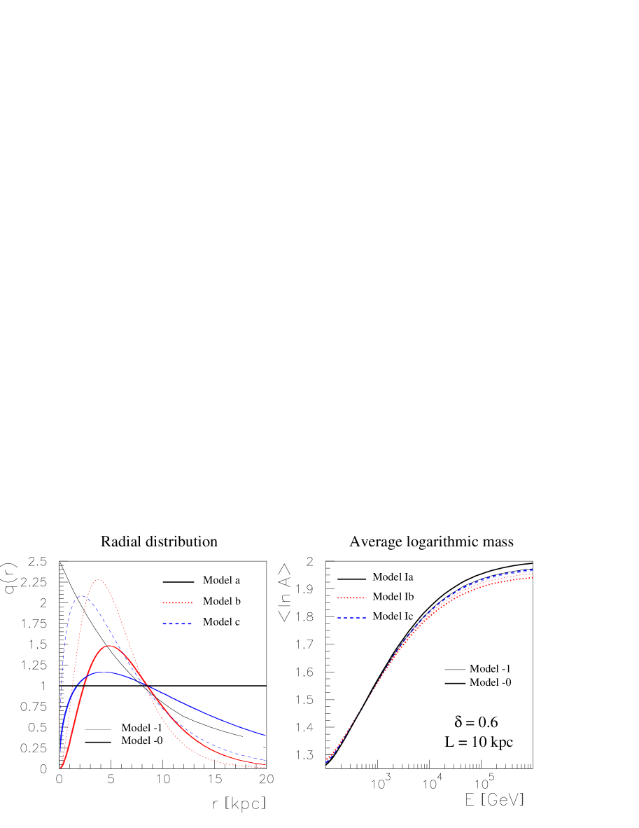
Figure 4: Left panel: representation of the three radial distribution of sources: solid lines are for constant distribution (models a), dotted lines are for Case & Batthacharia (models b) and dashed lines are for Strong & Moskalenko (models c); $q(r)$ is evaluated (see Tab. 5) with (models -1, thin line) or without (models -0, thick line) metallicity gradient. Right panel: average logarithmic mass (model I, $\delta=0.6$, $L=10$ kpc) for the six cases presented on left panel.

Other curves correspond to the evaluation of the pure geometrical effects. Both radial distribution (model a,b,c) and metallicity gradient (model 0,1) are separatly presented. In fact, comparing curve Ia-0 and Ia-1, we could conclude prematuraly that metallicity effect plays a role in the evolution of $\langle\ln A\rangle$. However, when the radial distribution of sources is correctly taken into account, metallicity only has a little additional effect (compare curves Ib-0 and Ib-1). Finally, the impact of metallicity is more or less pronounced depending of the distribution $q(r)$ chosen. Nevertheless, as was correctly guessed in Sec. 2.3, (i) metallicity effect is of little importance and (ii) total geometrical effects correspond to an additional change of at most 5% compare to a non geometrical model. Furthermore, Fig. 4 corresponds to a halo scale height $L=10$ kpc, for which the effects are maximized. For $L=3$ kpc, these geometrical effects are completely negligible.

5.2 Effects of propagation and source spectra

Fig. 5 (left panel) shows that the cosmic ray composition is very sensitive to the diffusion parameters, the strongest dependence being that of the diffusion power spectrum $\delta$ (the fixed point around 500 GeV is just an artifact due to the normalization adopted). Note that the asymptotic diffusive regime is reached faster for larger values of $\delta$. We checked that the influence of the parameter $L$ is minor compared to $\delta$’s.

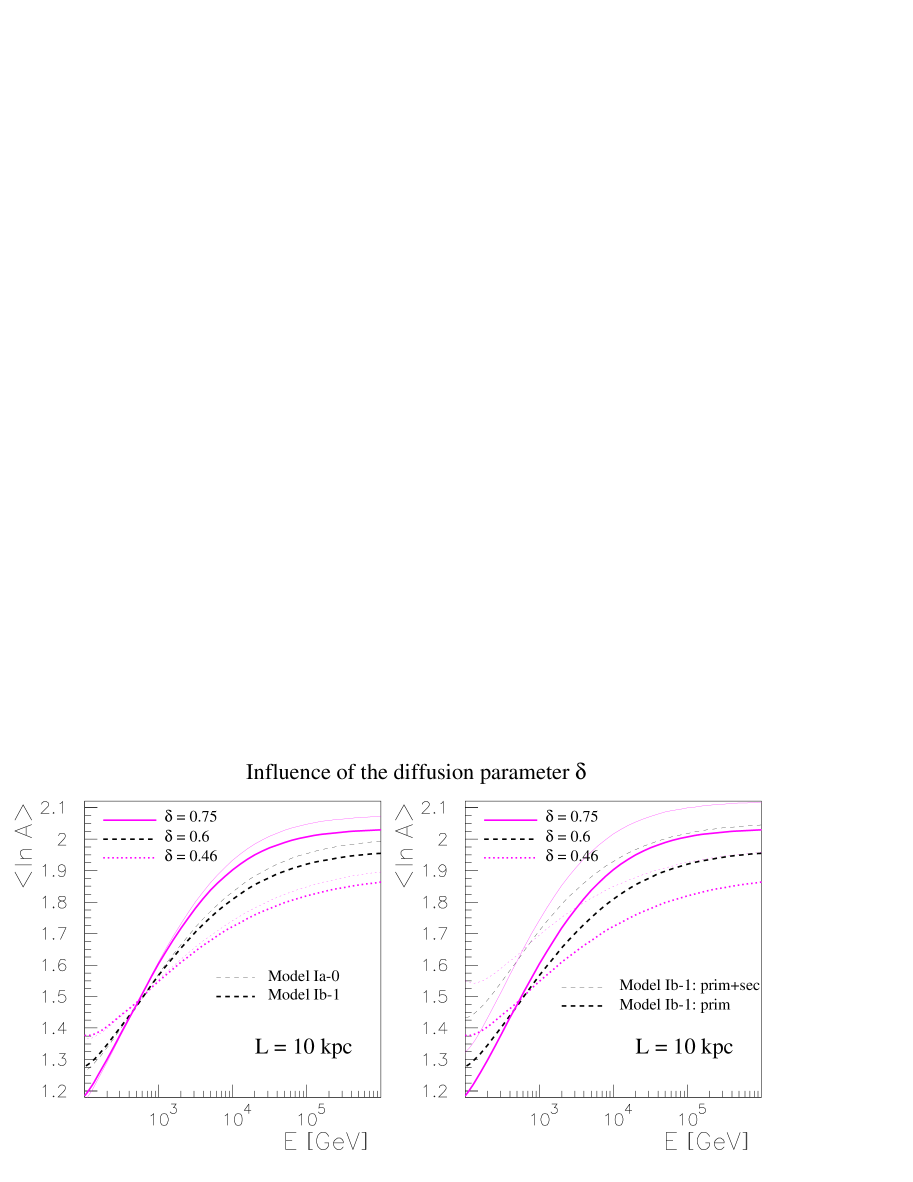
Figure 5: Average logarithmic mass (model I, $L=10$ kpc) for three values of the diffusion coefficient slope $\delta$. Left panel displays these three values for two cases, (i) model Ia-0 (no geometrical effects, thin line) and (ii) model Ib-1 (Case & Bhattacharia’s q(r) with $\nabla[{\rm Fe}/{\rm H}]=-0.05$ dex kpc^-1, thick line). Right panel shows for Model Ib-1 the same three $\delta$ values but introducing the distinction between $\langle\ln A\rangle$ evaluated (i) with primary species only (thick line), (ii) with all primary and secondary nuclei (thin line).

We note that secondary contribution (nuclei produced by spallation of the main primary species) is important (right panel). In particular, when making the junction between direct measurements and ground arrays, these secondaries are almost never taken into account in the calculation of the average logarithmic mass, whereas they are implicitly counted in air showers data (their presence in the reconstructed quantity $\langle\ln A\rangle$ is more questionable [8]). This question is related to the ability of obtaining a confident normalization of $\langle\ln A\rangle$ with data from nuclear interaction models, e.g. [42].

The impact of the spectral difference between protons (slope $\alpha_{\rm p}$) and other species (slope $\alpha_{\rm Z>1}\equiv\alpha$) is illustrated in Fig. 6 (left panel) showing an increase of the mass composition with $\alpha_{\rm p}-\alpha$.

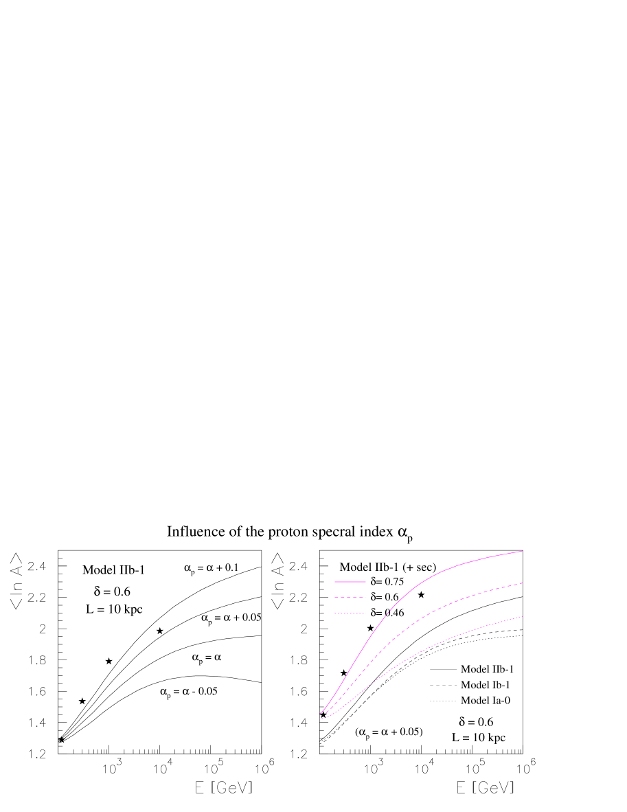
Figure 6: Left panel: average logarithmic mass (model IIb-1, $\delta=0.6$, $L=10$ kpc) for various values of cosmic ray proton spectral index $\alpha_{\rm p}$ (see Tab. 3). Right panel: summary of the various effects investigated in this paper for primary species, i.e pure propagation effect (Ia-0) + geometrical effect (Ib-1) + spectrum effect (IIb-1). The three upper curves correspond to three $\delta$ where secondary contributions are taken into account in Model IIb-1 ($\alpha_{\rm p}=\alpha+0.05$). Stars are values of $\langle\ln A\rangle$ measured in direct experiments (taken from Fig. 29 of [1]) interpolated from their original normalization to our 100 GeV normalization value.

The right panel summarizes the astrophysical effects studied here in the framework of a diffusion model: conclusions are similar to what was drawn in Sec. 2: pure propagation effects (Ia-0, dotted line) are mostly responsible for the increase of $\langle\ln A\rangle$ vs energy, geometrical effects (Ib-1, dashed line) are less significant, and source effects (IIb-1, solid line) turn from an almost asymptotically constant $\langle\ln A\rangle$ into a constant enhancement of the same quantity. The three upper curves demonstrate importance of the diffusion power spectrum $\delta$ and emphasize the role of the secondaries in the normalization of the average logarithmic mass. We also display the average logarithmic mass as measured by experiments (stars). We renormalize to the observations at 100 GeV. We see that a difference $\alpha_{\rm p}-\alpha>0$ or/and large values of $\delta$ are preferred.

5.3 Combination of all previous effects with a model for the knee

In Fig. 7, we generate the knee either with a break at a fixed rigidity, i.e $E_{\rm knee}=Z\times 4$ PeV, or at a fixed total energy per nucleus i.e $E_{\rm knee}=A\times 4$ PeV. The possibility of a break at a single energy is not considered because it exhibits a very sharp break in all-particle spectrum not present in data.

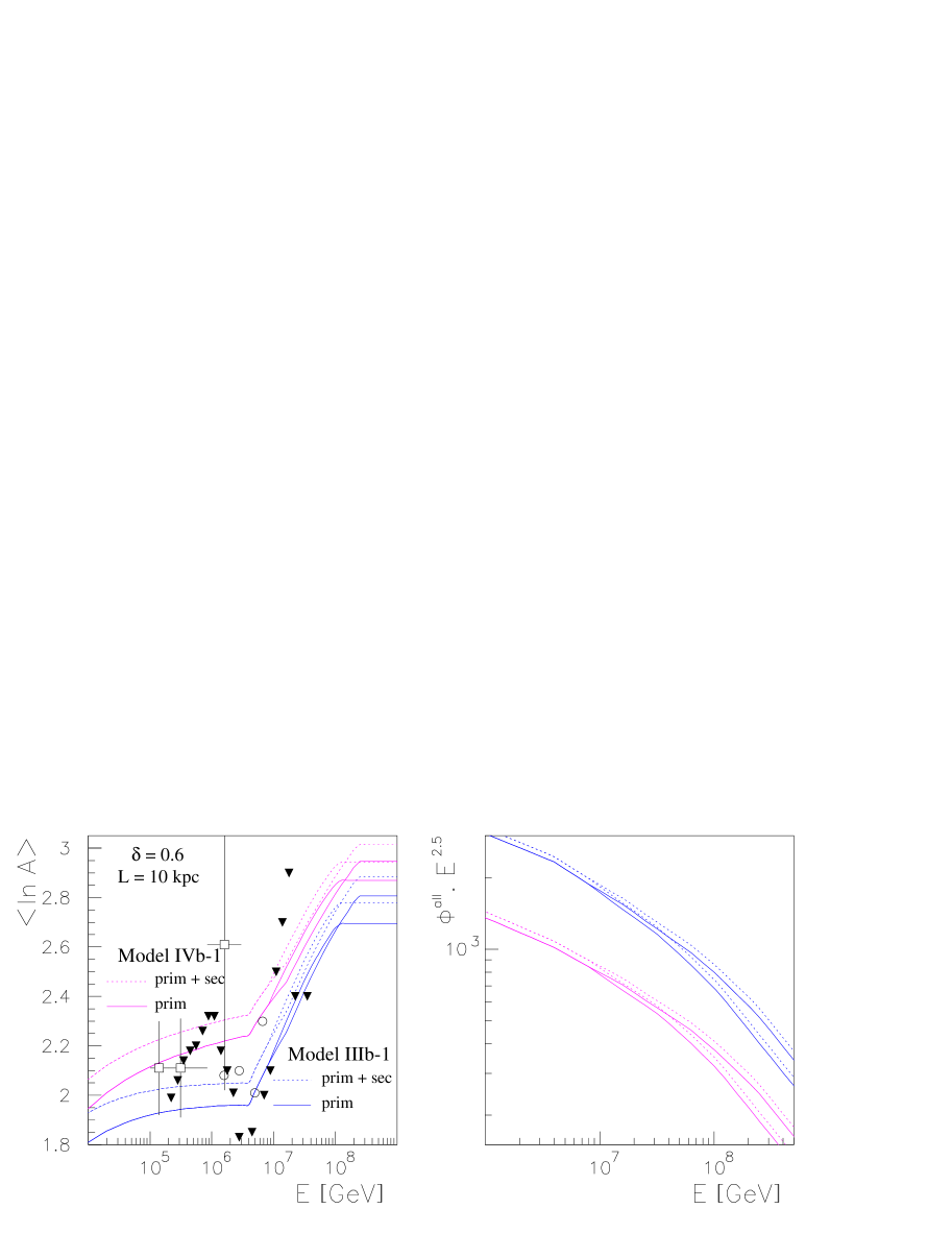
Figure 7: Average logarithmic mass (left panel) and all-particle spectrum (right panel) for Model IIIb-1 and IVb-1 with a break either in rigidity ($R=4$ PeV) or in total energy per nucleus (E/nuc $=4$ PeV). Solid lines correspond to primaries only, whereas dotted lines correspond to primaries plus secondaries. In the right panel, fluxes for Model IVb-1 have been divided by two in order to avoid the overlap with Model IIIb-1. For illustrative purpose, some data from ground arrays have been displayed: triangles are CASABLANCA’s data with Monte-Carlo hdpm [42], empty circles are from KASCADE collaboration with qgsjet simulation [8] (empty squares are from JACEE direct experiment; RUNJOB data plus some JACEE data are lower than 1.8 and do not appear on the graph, see [1]).

Fig. 7 displays the resulting curves for the two models IIIb-1 and IVb-1 that only differ in their spectral indexes below the knee ($\alpha_{\rm p}-\alpha=0.05$ for model IVb-1 and $\alpha_{\rm p}-\alpha=0.$ for IIIb-1). Compared to the results of the two components model (see Sec. 3), we remark both in $\langle\ln A\rangle$ and $\Phi^{\rm all}$ some additionnal bifurcations generated by the helium component with a second even smoother transition provided by the CNO group. If these effects are not very relevant for the average mass composition, they hamper the interpretation of the transition from one regime to the other in the all-particle spectrum data. Secondaries smooth even more these transitions. They are also important for normalization of $\langle\ln A\rangle$. The two cases $E_{\rm knee}=Z\times 4$ PeV and $E_{\rm knee}=A\times 4$ PeV could be differentiated mostly through the all-particle spectrum. Finally, the bigger the difference between proton slope and other species before the knee, the smoother the bump in $\langle\ln A\rangle$.

Before concluding, we would like to make a brief comment on Swordy’s model [67]: in the latter, an enhancement of light nuclei is predicted before the usual enrichment in heavier nuclei at the knee (some data can support this upturn, e.g. CASABLANCA’s data, see Fig. 7). However, this requires a change in diffusion (i.e $\Delta\delta<0$ because $\Phi\propto R^{-(\gamma=\alpha+\delta)}$) at an energy smaller than the knee’s, so that it should produce a bump visible in all-particle spectrum: the larger $\Delta\delta$, the sharper the bump, and moreover a larger value of $\Delta\alpha$ is then necessary to reproduce the all-particle spectrum at the knee. Thus, if position and sharpness of this change in diffusive regime (quite constrained by all-particle spectra) is not theoritically excluded, it requires to be extremely fine tuned. Anyway, this model along with our theoretical predictions cannot be tested due to the large data scattering (see Fig. 7).

The best clues up to now about the knee puzzle come from spectral analysis: for example the KASCADE collaboration [68] find that the all-particle spectrum exhibits a knee ($\Delta\gamma\sim 0.2-03$) around 4 PeV, but that this knee is seen only in their light ion subsample for which $\Delta\gamma\sim 0.5$. As regards the heavy ions, they find no changes in the region 1 – 10 PeV but the slope below the knee is smaller than that of light component. If this observation is confirmed, the average logarithmic mass is likely to evolve as depicted in our Model IVb-1.

5.4 Concluding remarks

We have presented an analysis of the phenomena that affect the chemical cosmic ray composition up to highest “Galactic” energies. Several astrophysical effects have been considered and geometrical effects have been found to play a minor role, while propagation effects (mostly selective destruction in flight of heavy nuclei) drive this evolution up to the knee where they cease to be effective. A difference between the source spectrum of protons and other ions lead to a constant enhancement of $\langle\ln A\rangle$ up to the knee and ceases if the slopes above the knee are similar for all species. In the framework of a simple break in rigidity (or total energy per nucleon), a bump in the chemical composition occurs at the knee, but the larger the spectral difference between protons and other species, the smoother the bump. The secondary species induce an enhancement in $\langle\ln A\rangle$ of about 15%. As a by-product, our study validates the approach recently used in [2], i.e we demonstrated that above PeV energy, a propagation model including only sources and diffusion is relevant. Finally, the main problem of the diffusive problem is the normalization of the fluxes. It could be improved thanks to a better determination of the propagation parameters with more precise low energy data.

References

- [1] A.V. Apanasenko et al., Astropart. Phys. 16 (2001) 13.
- [2] Y. Shirasaki et al., Astropart. Phys. 15 (2001) 357.
- [3] W.I. Axford, Astrophys. J. Suppl. S. 90 (1994) 937.
- [4] G. Schatz, Astropart. Phys. 17 (2002) 13.
- [5] B. Wiebel–Sooth and P.L. Biermann, in: invited chapter for Landolt-Börnstein (Springer Publ. Comp., 1999), vol VI/3c, p. 37-90.
- [6] K. Bernlöhr, W. Hofmann, G. Leffers, V. Matheis, M. Panter and R. Zink, Astropart. Phys. 8 (1998) 253.
- [7] S.P. Swordy and D.B. Kieda, Astropart. Phys. 13 (2000) 137.
- [8] T. Antoni et al., Astropart. Phys. 16 (2002) 245.
- [9] D.B. Kieda, S.P. Swordy and S.P. Wakely, Astropart. Phys. 15 (2001) 287.
- [10] M.D. Roberts, Astropart. Phys. 12 (2000) 239.
- [11] A. Linder, Astropart. Phys. 8 (1998) 235.
- [12] M. Amenomori et al., Phys. Rev. D 62 (2000) 112002.
- [13] S.P. Swordy et al., astro-ph/0202159 (2002).
- [14] D. Maurin, F. Donato, R. Taillet and P. Salati, Astrophys. J. 555 (2001) 585.
- [15] J.A. Simpson, Ann. Rev. Nucl. Part. Science 33 (1983) 323.
- [16] W.R. Webber, Space Sci. Rev. 81 (1997) 107.
- [17] A.W. Strong, I.V. Moskalenko and O. Reimer, Astrophys. J. 537 (2000) 763.
- [18] F.C. Jones, A. Lukasiak, V.S. Ptuskin and W.R. Webber, Astrophys. J. 547 (2001) 264.
- [19] B. Wiebel–Sooth, P.L. Biermann and H. Meyer, Astron. & Astrophys. 330 (1998) 389.
- [20] W.R. Webber, J.C. Kish, J.M. Rockstroh, Y. Cassagnou, R. Legrain, A. Soutoul, O. Testard and C. Tull, Astrophys. J. 508 (1998) 940.
- [21] R.F. Carlson, Atom. Data & Nuc. Data Tab. 63 (1996) 93.
- [22] P.O. Lagage and C.J. Cesarsky, Astron. & Astrophys. 125 (1983) 249.
- [23] J.R. Jokipii and G.E. Morfill, Astrophys. J. 290 (1985) L1.
- [24] J.R. Jokipii and G.E. Morfill, Astrophys. J. 312 (1987) 170.
- [25] K.S. Cheng and X. Chi, Astron. & Astrophys. 306 (1996) 326.
- [26] W. Bednarek and R.J. Protheroe, Astropart. Phys. 16 (2002) 397.
- [27] A.D. Erlykin and A.W. Wolfendale, Astron. & Astrophys. 356 (2000) L63.
- [28] A.D. Erlykin, M. Lipski and A.W. Wolfendale, Astropart. Phys. 8 (1998) 283.
- [29] J. Candia, L.N. Epele and E. Roulet, Astropart. Phys. 17 (2002) 23.
- [30] E.G. Klepach, V.S. Ptuskin and V.N. Zirakashvili, Astropart. Phys. 13 (2000) 161.
- [31] A.M. Bykov and I.N Toptygin, Astron. Lett. 27 (2001) 625.
- [32] A.R. Bell and S.G. Lucek, MNRAS 321 (2001) 433.
- [33] S.G Lucek and A.R. Bell, MNRAS 314 (2000) 65.
- [34] P.L. Biermann, Astron. & Astrophys. 271 (1993) 649.
- [35] P.L. Biermann, T.K. Gaisser and T. Stanev, Phys. Rev. D 51 (1995) 3450.
- [36] D.E. Ellison, Proc. 23rd Int. Cosmic Ray Conf., Calgary, Canada, vol. 2 (1993) p. 219.
- [37] J. Clem, W. Droege, P.A. Evenson, H. Fischer, G. Green, D. Huber, H. Kunow and D. Seckel, Astropart. Phys. 16 (2002) 387.
- [38] M.A.K. Glasmacher et al., Astropart. Phys. 12 (1999) 1.
- [39] F. Arqueros et al., Astron. & Astrophys. 359 (2000) 682.
- [40] M. Amenomori et al., Astrophys. J. 461 (1996) 408.
- [41] M. Aglietta et al., Astropart. Phys. 10 (1999) 1.
- [42] J.W. Fowler, L.F. Fortson, C.C.H Jui, D.B. Kieda, R.A. Ong, C.L. Pryke, and P. Sommers, Astropart. Phys. 15 (2001) 49.
- [43] Y. Shirasaki and F. Kakimoto, Astropart. Phys., 15 (2001) 241.
- [44] V. Topor Pop, M. Gyulassy and H. Rebel, Astropart. Phys. 10 (1999) 211.
- [45] V.N. Bakatanov, Yu.F. Novosel’tsev and R.V. Novosel’tseva, Astropart. Phys. 12 (1999) 19.
- [46] T. Abu-Zayyad et al., Astropart. J. 557 (2001) 686.
- [47] V.S. Berezinskii, S.V. Bulanov, V.A. Dogiel, V.L. Ginzburg and V.S Ptuskin, Astrophysics of Cosmic Rays (Amsterdam, North–Holland, 1990)
- [48] A. Barrau, G. Boudoul, F. Donato, D. Maurin, P. Salati and R. Taillet, Astron. & Astrophys. 388 (2002) 676.
- [49] F. Donato, D. Maurin, P. Salati, A. Barrau, G. Boudoul and R. Taillet, Astrophys. J., 563 (2001) 172.
- [50] F. Donato, D. Maurin and R. Taillet, Astron. & Astrophys. 381 (2002) 539.
- [51] V.S. Ptuskin, S.I. Rogovaya, V.N. Zirakashvili, L.G. Chuvilgin, G.B. Khristiansen, E.G. Klepach and G.V. Kulikov, Astron. & Astrophys. 268 (1993) 726.
- [52] K. Kodaira, PASJ 26 (1974) 255.
- [53] G.L. Case and D. Bhattacharya, Astrophys. J. 504 (1998) 761.
- [54] G.L. Case and D. Bhattacharya, Astron. & Astrophys. Suppl. 120 (1996) 437.
- [55] A.W. Strong and I.V. Moskalenko, Astrophys. J. 509 (1998) 212.
- [56] W.J. Maciel, in: IAU Symp. 180, Planetary Nebulae, eds. H.J. Habing and H.J.G.L.M Lamers (Kluver, Dordrecht, 1997) p. 397.
- [57] C.A. Gummersbach, A. Kaufer, D.R. Scäfer, T. Szeifert and B. Wolf, Astron. & Astrophys. 338 (1998) 881.
- [58] C. Chiappini, F. Matteucci and D. Romano, Astrophys. J. 554 (2001) 1044.
- [59] S.M. Andrievsky et al., Astron. & Astrophys. 381 (2002) 32.
- [60] W.R.J. Rolleston, S.J. Smartt, P.L. Dufton and R.S.I. Ryans, Astron. & Astrophys. 363 (2000) 537.
- [61] W.J. Maciel and C. Quireza, Astron. & Astrophys. 345 (1999) 629.
- [62] G. Carraro, Y.K. Ng and L. Portinari, MNRAS 296 (1998) 1045.
- [63] A. Afflerbach, E. Churchwell and M.W. Werner, Astrophys. J. 478 (1997) 190.
- [64] J.J. Engelmann et al. Astron. & Astrophys. 233 (1990) 96.
- [65] ams Collaboration: J. Alcaraz et al., Phys. Lett. B 490 (2000) 27.
- [66] ams Collaboration: J. Alcaraz et al., Phys. Lett. B 494 (2000) 193.
- [67] S.P. Swordy, Proc. 24th Int. Cosmic Ray Conf., Roma, Italy, vol. 3 (1995) p. 697.
- [68] T. Antoni et al., Astropart. Phys. 16 (2002) 373.