Atomic Polarization and the Hanle Effect

Abstract

This article presents an introduction to optical pumping, atomic polarization and the Hanle effect in weakly magnetized stellar atmospheres. Although the physical processes and the theoretical framework described here are of interest for applications in a variety of astrophysical contexts (e.g. scattering polarization in circumstellar envelopes and polarization in astronomical masers), the article focuses mainly on the quest for understanding the physical origin of the linearly polarized solar limb spectrum. It considers also the development of the Hanle effect as a reliable diagnostic tool for making feasible new advances in solar photospheric and chromospheric magnetism. Particular emphasis is given to a rigorous modeling of polarization phenomena as the essential link between theory and observations. Some of the most recent advances in this field are presented after carefully explaining how the various radiation pumping mechanisms lead to atomic polarization in the absence and in the presence of weak magnetic fields.

Instituto de Astrofísica de Canarias, 38200 La Laguna, Tenerife, Spain. (e-mail: jtb@iac.es)

1. Introduction

Probably the first thing I should point out is that the “second solar spectrum” is nothing but the observational signature of the “order” that exists in the atomic system. This “atomic organization” is what we call atomic polarization (i.e. the existence of population imbalances among the sublevels of any given degenerate atomic or molecular level and/or the presence of quantum interferences or coherences between any given pair of sublevels, even among those pertaining to different levels). But, what is forcing the ions, atoms and molecules of the stellar atmospheric plasma to behave this way? As we shall see below, the atomic polarization is the result of a transfer process of “order” from the radiation field to the atomic system. It is thus natural that the logical structure of this review article is as follows: quantification of the “order” of the radiation field (Section 3), quantification of the “order” of the atomic system (Section 4) and transfer of “order” from the radiation field to the atomic system (Section 5).

The interesting point for solar surface magnetism is that weak magnetic fields (from 1 milligauss to 100 gauss, approximately) modify the atomic polarization via the Hanle effect. However, in order to develop the Hanle effect as a reliable diagnostic tool of weak magnetic fields it is extremely important to fully understand the reference case of non-magnetic scattering polarization. With this motivation in mind Section 6 presents, for the first time, results of multilevel scattering polarization calculations taking fully into account all the relevant pumping mechanisms and the transfer of atomic polarization among all the levels involved. After considering in some detail the unmagnetized reference case a few examples in Section 7 will show how weak magnetic fields (from a few milligauss to a few gauss) modify the atomic polarization of multilevel atomic systems. Finally, Section 8 gives our concluding remarks. Section 2 is mainly dedicated to introducing the subject to those readers approaching the Hanle effect for the first time.

2. Introduction to the Hanle effect

This section is of introductory nature. Similar and additional information may be found in Hanle’s (1924) paper on “Magnetic Effects on the Polarization of Resonance Fluorescence”, in the classical monograph of Mitchell and Zemansky (1934), in Landi Degl’Innocenti’s (1992) contribution to the first IAC Winter School, in the book edited by Moruzzi and Strumia (1991), and in the papers by Landolfi & Landi Degl’Innocenti (1986) and by Manso Sainz & Trujillo Bueno (1999). Other reviews and keynote articles related to this topic (including the determination of magnetic fields in solar prominences) can be found in Landi Degl’Innocenti (1990), Stenflo (1994), Faurobert-Scholl (1996) and Trujillo Bueno (1999). For a discussion concerning the possibilities of the Hanle effect for the detection of magnetic fields in stellar winds see Ignace et al. (1997).

2.1. Hanle’s “Doktorarbeit”

The story began in 1923 when Wilhelm Hanle of Göttingen University published the first correct interpretation of a previously observed phenomenon related to the effect of a weak magnetic field on the linear polarization of the spectral-line radiation scattered by mercury vapor illuminated anisotropically (see Hanle 1923; 1924). With respect to the linear polarization corresponding to the zero magnetic field case, the observed influence of a weak magnetic field (of the order of 1 gauss) was a rotation of the plane of linear polarization (observed experimentally by Hanle himself) and a depolarization (clearly pointed out previously by Wood and Ellett in 1923). This so-called Hanle effect played a fundamental role in the development of quantum mechanics, since it led to the introduction and clarification of the concept of coherent superposition of pure states (see Bohr 1924; Hanle 1924, 1925; Heisenberg 1925). The Hanle effect is directly related to the generation of coherent superposition of degenerate Zeeman sublevels of an atom (or molecule) by a light beam. As the Zeeman sublevels are split by the magnetic field, the degeneracy is lifted and the coherence (and, in general, also the population imbalances among the sublevels) are modified. As we shall illustrate below in the context of the solar polarized spectrum, this gives rise to a characteristic magnetic-field dependence of the linear polarization of the scattered light that is finding increasing application as a diagnostic tool for magnetic fields in astrophysics (see Astrophysical Spectropolarimetry, edited by Trujillo Bueno, Moreno Insertis and Sánchez 2001).

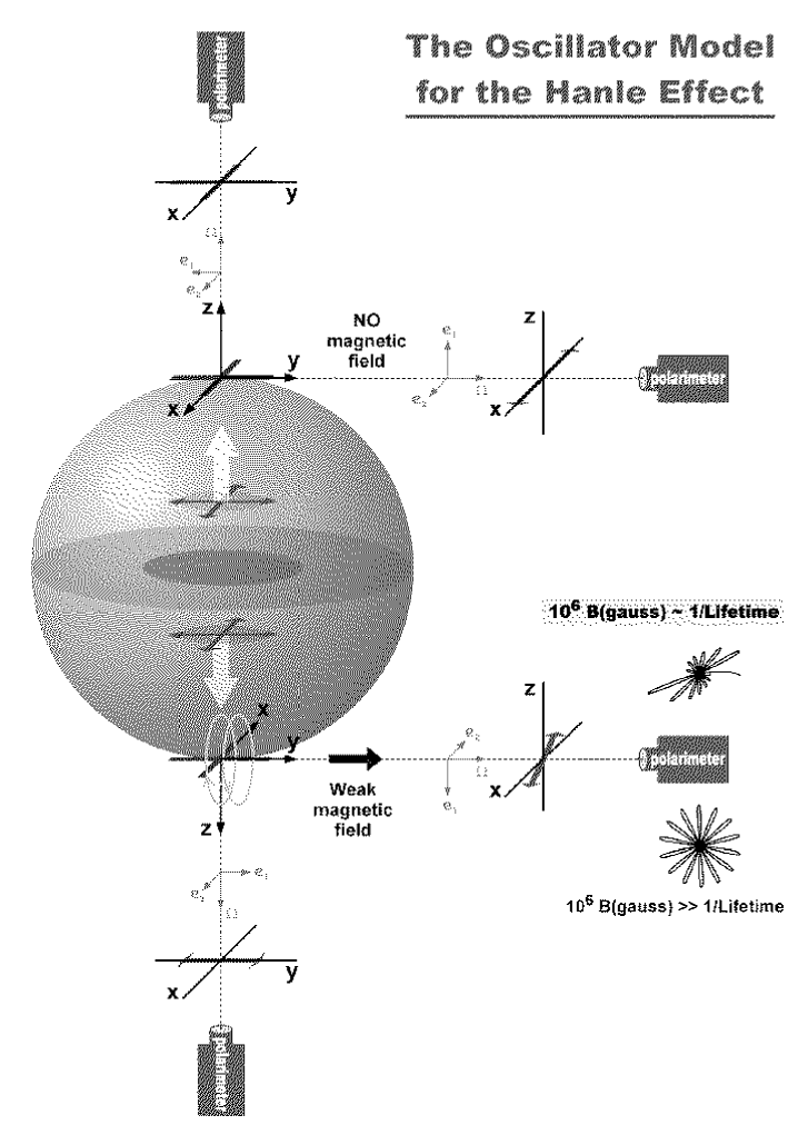
Figure 1.: The oscillator model for the Hanle effect.

2.2. The oscillator model for the Hanle effect

Figure 1 is aimed at introducing the most basic ideas behind scattering polarization and the Hanle effect (see also Landi Degl’Innocenti, 1992). It is based on the classical interpretation of the Hanle effect for a triplet-type transition originating between a ground level with total angular momentum $J_{l}=0$ and an excited level with $J_{u}=1$. The atom is treated as a negative charge oscillating with angular frequency $\omega_{0}$ and with a damping constant $\gamma$ given by the inverse of the lifetime of the excited atomic level (e.g. the upper level of a resonance line transition has a lifetime $t_{\rm life}{\approx}1/A_{ul}$, $A_{ul}$ being the Einstein coefficient for spontaneous emission). In solar-like atmospheres $1/t_{\rm life}\ll{\Delta\omega}_{\rm line}$, with ${\Delta\omega}_{\rm line}$ the width of the spectral line under consideration.

As seen in Fig. 1, we are assuming that the atoms in the outer layers of the solar atmosphere are being illuminated by an unpolarized radiation field, which we are approximating by a unidirectional beam propagating in the radial direction. The unpolarized character of this radiation beam is indicated in Fig. 1 by two perpendicular uncorrelated components of the electric field of the wave. Single-scattering events take place and the light polarization is measured for both forward scattering and $90$ degree scattering as shown in Figure 1.

Consider first the observation of the “north solar pole”, where we have assumed in Fig. 1 that there is no magnetic field (i.e. there is no Lorentz force influencing the motion of the oscillating electron). Under these circumstances the atom can be represented by three independent linear oscillators vibrating at angular frequency $\omega_{0}$ along the axes of the reference system. As indicated in Fig. 1, only the $x$ and $y$ oscillators are excited by the incident beam. The two excited oscillators radiate independently and decay radiatively with a damping constant $\gamma=1/t_{\rm life}$. If we observe along the direction of the incident beam (forward scattering case) we find that the radiation is obviously unpolarized. However, observing at 90^∘ one finds that the radiation is linearly polarized along the $x$-axis, simply because the $y$-oscillator is seen pole-on. If we choose the positive reference direction for the Stokes $Q$ parameter along the $x$-axis, we find $Q=I$ and $U=0$. Note that the same conclusion is obviously reached if the vibration of the $x$-oscillator is considered as that resulting from the coherent superposition of two counter-rotating circular oscillators, which are oscillating in phase with respect to each other at frequency $\omega_{0}$ in the $x$$-$$z$ plane.

Consider now the observations of the “south solar pole”, where we have assumed in Fig. 1 the presence of a weak magnetic field parallel to the solar surface and orientated along the $y$-axis. We have now to take into account the influence of the Lorentz force on the motion of the bound electron. The result is that the atom cannot be interpreted as three independent linear oscillators, but as a linear oscillator parallel to the magnetic field and two counter-rotating circular oscillators in the $x$$-$$z$ plane oscillating at angular frequencies $\omega_{0}+\omega_{\rm L}$ and $\omega_{0}-\omega_{\rm L}$, where $\omega_{\rm L}\,=\,8.79\,\times 10^{6}\,B({\rm gauss})$ is the Larmor angular frequency (with $B({\rm gauss})$ indicating that the magnetic field is to be given in gauss). The resulting trajectory of the electron in the $x$$-$$z$ plane is given by

$$x(t)=A\,e^{-{\gamma}t/2}{\rm cos}(\omega_{\rm L}t){\rm cos}(\omega_{0}t),$$ (1)

$$z(t)=A\,e^{-{\gamma}t/2}{\rm sin}(\omega_{\rm L}t){\rm cos}(\omega_{0}t).$$ (2)

The trajectory described by these equations is an oscillation at frequency $\omega_{0}$, with an amplitude that decays exponentially with a characteristic damping time given by $t_{\rm life}=1/\gamma$, and such that its oscillation axis is rotating at frequency $\omega_{\rm L}$. If the Zeeman splitting is sufficiently large so as to have $\omega_{\rm L}\gg 1/t_{\rm life}$ (which can occur having still $\omega_{\rm L}\,{\ll}\,{\Delta\omega}_{\rm line}$) the oscillation axis can rotate several times before the oscillation amplitude is affected by the damping. The bound electron describes in the $x$$-$$z$ plane the “daffodil” pattern shown in the lower part to the r.h.s. of Figure 1. Under these circumstances we will see totally unpolarized radiation for the 90 degree scattering case (i.e. for observation at the limb), but the maximum possible amount of linear polarization along the $y$-axis for forward scattering (i.e. for disc-centre observation).

However, when the Zeeman splitting is similar to the natural width of the atomic level (i.e. when $\omega_{\rm L}{\approx}1/t_{\rm life}$) the oscillation axis rotates through an angle $\alpha$ within the characteristic damping time. The bound electron describes in the $x$$-$$z$ plane the “rosette” shown in Figure 1. For the 90 degrees scattering case (i.e. for observation at the limb) the $y$-oscillator is seen pole-on and, therefore, the observed polarization simply reflects the weighted average of the above-mentioned “rosette” pattern. With respect to the previous unmagnetized “north-pole case”, we now get (for observation at the limb) a depolarization and a rotation of the polarization plane (i.e. we now have a smaller Stokes $Q$ value and a non-zero Stokes $U$ signal). This rotation is counterclockwise for a magnetic field pointing toward the observer, as in Fig. 1, but clockwise if the magnetic field points in the opposite direction. Accordingly, for a mixed-polarity magnetic field topology within the spatio-temporal resolution element of the observations, the measured Stokes $U$ parameter would be zero, while we would still be able to detect the depolarization effect by measuring Stokes $Q$. For a disc-centre observation (forward scattering case) we would get (for the magnetic field orientation of Fig. 1) a net linear polarization signal along the $y$-axis, but of smaller amplitude than that corresponding to the previous $\omega_{\rm L}\gg 1/t_{\rm life}$ forward-scattering case.

Finally, it is also of interest to consider the “south pole” magnetized case, but assuming that the weak magnetic field is now orientated along the $x$-axis. It is easy to understand that all remains unchanged with regard to the forward scattering case (with the exception that now the observed linear polarization is along the $x$-axis, i.e. again along the magnetic field direction). However, for the limb observation we would only see the depolarization effect (i.e. a Stokes $Q$ signal decreasing with the magnetic field, but $U=0$ always). Moreover, the Stokes $Q$ signal does not vanish completely once the magnetic field becomes sufficiently large so as to have $\omega_{\rm L}\gg 1/t_{\rm life}$. Figure 2 corresponds to the situation of a magnetic field which is always orientated along the $x$-axis. Note that a magnetic field parallel to the solar surface and with an intensity in the saturated regime (i.e. $\omega_{\rm L}\gg 1/t_{\rm life}$ or $\Gamma\gg 1$) leads to a linear polarization amplitude for disc-centre observations that is an order of magnitude smaller than that corresponding to the unmagnetized reference case ($\Gamma=0$) for an observation close to the solar limb ($\mu=0.1$). Given the weakness of the “predicted” disc-centre polarization signals, two spectral lines of possible interest for a disc-centre Hanle-effect observational search of horizontal chromospheric fields would be the Ca I 4227 Å  line and the D₂ line of Ba II at 4554 Å .

Figure 2.: Hanle-effect radiative transfer simulation for limb and disc-centre observations. The figure shows the emergent fractional linear polarization versus the line frequency in units of the Doppler width. The positive reference-direction for the Stokes $Q$ parameter is along the unit vector ${\bf e_{2}}$ of Figure 1. Assumptions: triplet-type transition of a two-level model atom with inelastic collisional destruction probability $\epsilon=10^{-4}$ in an isothermal model atmosphere and neglecting depolarizing elastic collisions. The magnetic field is parallel to the stellar surface and orientated along the $x$-axis of Figure 1. The simulated observations are as in Fig. 1 (for $\mu=1$, but for $\mu=0.1$ instead of $\mu=0$). The intensity of the magnetic field is quantified by $\Gamma=8.79{\times}10^{6}\,B{\rm(gauss)}\,g_{J}/A_{ul}$, with $g_{J}=1$.

2.3. The basic Hanle-effect formula

As we have seen, the Hanle effect produces a modification of the linear polarization signals (quantified by the Stokes $Q$ and $U$ parameters) with respect to the reference case of non-magnetic scattering polarization. This occurs in a parameter domain in which the transverse Zeeman effect is practically ineffective. The Hanle effect is sensitive to magnetic fields such that the corresponding Zeeman splitting is comparable to the inverse lifetime of the lower or the upper atomic levels involved in the line transition under consideration. The basic approximate formula to estimate the maximum magnetic field intensity $B$ (measured in gauss) to which the Hanle effect can be sensitive is

$$10^{6}\,\,{B}\,\,g_{J}\,\,\approx\,\,1/t_{\rm life}\,\,,$$ (3)

where $g_{J}$ and $t_{\rm life}$ are, respectively, the Landé factor and the lifetime of the atomic level under consideration (which can be either the upper or the lower level of the chosen spectral line transition). Depending on the astrophysical plasma under consideration, on the intensity and orientation of its magnetic field and on the spectral line chosen, we may find different Hanle-effect regimes. The most familiar one to astrophysicists in general is the “upper-level Hanle effect”, in which only the upper-level coherences are modified by the action of the magnetic field. However, we may also have a “lower-level Hanle effect” regime in which only the lower-level coherences are sensitive to the field. The most general Hanle-effect takes place when the magnetic field affects the coherences of both levels simultaneously. Obviously, this dichotomy between an upper-level and a lower-level Hanle effect is only a suitable one if there exists a sizeable difference in the lifetimes of the lower and upper levels of the particular radiative transition. It certainly holds for solar spectral lines whose lower level is either the ground or a metastable level, as happens, for example, with the D-lines of Na I (Landi Degl’Innocenti 1998) or with the Mg I $b$ lines (Trujillo Bueno 1999). It is important to note that in the solar atmosphere (whose $T_{\rm eff}{\approx}5800$ K) the lifetime of a ground or metastable level is typically two orders of magnitude larger than the lifetime of the upper level. Therefore, for typical solar spectral lines the upper-level Hanle effect would be sensitive to magnetic fields of between 1 and 100 gauss, while the lower-level Hanle effect could in principle be used for diagnosing much weaker fields, i.e. fields between $10^{-3}$ and 1 gauss. Whether or not sub-gauss magnetic fields can actually exist in the highly conductive solar plasma is a question that most solar plasma physicists are inclined to answer negatively. The main result I aim at demonstrating in this article is that the “enigmatic” linear polarization signals observed by Stenflo et al. (2000) close to the solar limb in a number of chromospheric lines are undoubtedly due to the presence of atomic polarization in their metastable-level lower-levels. These observations of scattering polarization on the Sun have been confirmed recently (and extended to the Stokes $U$ and $V$ parameters) by Dittmann et al. (2001), Martínez Pillet et al. (2001) and by Trujillo Bueno et al. (2001) using different polarimeters attached to the Canary Islands solar telescopes. How such metastable-level atomic polarization can survive in the solar chromosphere is certainly a challenging question that I will also address in this paper. In particular, I will discuss briefly how a rigorous theoretical interpretation of this type of spectropolarimetric observations is giving us decisive new clues about the topology and intensity of the magnetic field of the “quiet” solar chromosphere.

Figure 3.: The Hanle effect versus the Zeeman effect. The figure shows the maximum polarization degree of a $J_{l}=0\,{\rightarrow}\,J_{u}=1$ resonance line (with $A_{ul}=10^{7}\ {\rm s}^{-1}$ and Doppler width ${\Delta{\nu}}_{\rm D}=10^{10}\ {\rm s}^{-1}$) versus the magnetic field intensity. The simulated observation is close to the limb ($\mu=0.1$) of the model atmosphere of Figure 2. The polarization signals are due either to the Zeeman effect (Z) or to the Hanle effect (H). The dashed–dotted line gives the sensitivity of the Hanle effect to a microturbulent and isotropic magnetic field. Note that for this kind of mixed-polarity scenario there is no Zeeman signal. The two other cases are for a magnetic field parallel to the stellar surface, and orientated either along the $x$-axis of Fig. 1 (curves with the symbol $\perp$) or along the $y$-axis (curves with the symbol $\parallel$). The polarimetric signals corresponding to the transverse Zeeman effect (see the solid line labelled Z($\perp$)) have been multiplied by a factor 10 to make them visible in the figure. Note that for magnetic field intensities greater than 10 gauss (i.e. for the saturated Hanle-effect regime where $\Gamma{\gg}1$) the “Hanle-effect signal” is only sensitive to the orientation of the magnetic field vector, but not to its intensity. This can occur for a Zeeman splitting which is still a very small fraction of the width of the spectral line. (From Manso Sainz & Trujillo Bueno 2001b).

2.4. The utility of the Zeeman effect

Before entering into details it is convenient to recall that the Zeeman effect is most sensitive in circular polarization (quantified by the Stokes $V$ parameter), with a magnitude that scales with the ratio between the Zeeman splitting and the width of the spectral line, and in a way such that the $V$ profile changes its sign for opposite orientations of the magnetic field vector. The longitudinal Zeeman effect in typical solar Fraunhofer lines is of course rather insensitive to sub-gauss magnetic fields. However, we should keep in mind that today’s state-of-the-art polarimeters are perfectly able to detect Stokes $V$ signals corresponding to a flux density of only a few gauss (see, e.g., Sánchez Almeida and Lites, 2000). Thus, unless this flux density is well below 1 gauss in the spatio-temporal resolution element of the observations, the longitudinal Zeeman effect itself should be considered of complementary diagnostic value to the Hanle effect. In any case, it is important to emphasize that the Hanle effect, contrary to the Zeeman effect, does indeed work in any topologically complex weak-field scenario (i.e. even if the net magnetic flux turns out to be exactly zero) by producing a modification of the linear polarization signals (with respect to the zero magnetic field reference case) that we can really “measure” if we succeed in rigorously modeling polarization signals due to multiple-scattering processes in the presence of weak magnetic fields. In conclusion, besides being useful for “measuring” magnetic fields in solar prominences, the Hanle effect offers a promising diagnostic tool for the investigation of weak photospheric fields with mixed polarities over small spatial scales and for the exploration of chromospheric magnetic fields (because chromospheric lines are generally broad and the magnetic fields of the solar chromosphere relatively weak). Figure 3 illustrates what has just been pointed out in relation to the diagnostic interest of the Hanle and Zeeman effects. A suitable illustration of the fact that the Hanle effect only operates in the Doppler core has been provided by Stenflo (1998) for the case of a $J_{l}=0\,{\rightarrow}\,J_{u}=1$ line transition.

3. How to quantify the order of the radiation field?

In the standard multilevel radiative transfer problem (see Mihalas, 1978) the only quantity related to the radiative line transitions that plays a role in the statistical equilibrium equations is:

$${\bar{J}^{0}_{0}}=\int{\rm d}x\oint\phi_{x}\frac{{\rm d}\vec{\Omega}}{4\pi}\,{{I_{x\vec{\Omega}}}},$$ (4)

where $x$ is the frequency measured from line centre in units of the Doppler width, $\phi_{x}$ the absorption line shape, $\vec{\Omega}$ the direction of propagation of the ray, and $I_{x\vec{\Omega}}$ the specific intensity of the radiation field, i.e. the Stokes $I$ parameter. Regardless of the dependence of the radiation field on frequency and direction this quantity (${\bar{J}^{0}_{0}}$) is always positive. Note also that $B_{lu}{\bar{J}^{0}_{0}}$ gives the contribution of the absorption process (between a lower level $l$ and an upper level $u$) to the natural width of the lower level “$l$” ($B_{lu}$ is the Einstein coefficient for such an absorption process). If this lower level is either the ground or a metastable level, its lifetime is $t_{\rm life}\,{\approx}\,1/B_{lu}{\bar{J}^{0}_{0}}$ if and only if the line transition $l\,{\rightarrow}\,u$ is among the strongest ones. This applies, for instance, to the lower-levels of the Mg $b$ lines, to the lower levels of the Ca ii IR-triplet, and to many other spectral lines in the solar spectrum. All such lower levels are metastable. As a result, their lifetimes are about two orders of magnitude larger than the lifetime of the upper levels of the above-mentioned spectral lines.

However, in the most general polarization transfer case, there are eight additional radiation field quantities that play a critical role in the statistical equilibrium equations (see Landi Degl’Innocenti, 1983). They are the spherical tensors ($\bar{J}^{K}_{Q}$) of the radiation field (with $K=1,2$ and $-K\,{\leq}\,Q\,{\leq}\,K$) and they are the quantities we choose to quantify the “order” of the radiation field:

$${{\bar{J}^{2}_{0}}}=\int{\rm d}x\oint\phi_{x}\frac{{\rm d}\vec{\Omega}}{4\pi}\frac{1}{2\sqrt{2}}\left[(3\mu^{2}-1){{I_{x\vec{\Omega}}}}+3(\mu^{2}-1){Q_{x\vec{\Omega}}}\right]\,,$$ (5)

$${{\bar{J}^{2}_{1}}}=\int{\rm d}x\oint\phi_{x}\frac{{\rm d}\vec{\Omega}}{4\pi}\frac{\sqrt{3}}{2}{{e^{i\chi}}}\sqrt{1-\mu^{2}}\,\left[-\mu\left({{I_{x\vec{\Omega}}}}+{{Q_{x\vec{\Omega}}}}\right)-i{{U_{x\vec{\Omega}}}}\right]\,,$$ (6)

$${{\bar{J}^{2}_{2}}}=\int{\rm d}x\oint\phi_{x}\frac{{\rm d}\vec{\Omega}}{4\pi}\frac{\sqrt{3}}{2}{{e^{2i\chi}}}\,\left[\frac{1}{2}(1-\mu^{2}){{I_{x\vec{\Omega}}}}-\frac{1}{2}(1+\mu^{2}){{Q_{x\vec{\Omega}}}}-i\mu{{U_{x\vec{\Omega}}}}\right]\,,$$ (7)

$${{\bar{J}^{1}_{0}}}=\int{\rm d}x\oint\phi_{x}\frac{{\rm d}\vec{\Omega}}{4\pi}\,\sqrt{\frac{3}{2}}\mu\,{{V_{x\vec{\Omega}}}}\,,$$ (8)

$${{\bar{J}^{1}_{1}}}=-\int{\rm d}x\oint\phi_{x}\frac{{\rm d}\vec{\Omega}}{4\pi}\,{{e^{i\chi}}}\,\sqrt{\frac{3}{2}}\sqrt{1-\mu^{2}}\,{{V_{x\vec{\Omega}}}}\,,$$ (9)

where the azimuthal angle $\chi$ and $\mu={\rm cos}\theta$ specify the orientation of each ray of direction $\vec{\Omega}$. The reference direction for the Stokes $Q$ and $U$ parameters is situated in the plane perpendicular to $\vec{\Omega}\,$ and lies in the plane containing $\vec{\Omega}$ and the $z$-axis. The ${{\bar{J}^{K}_{-Q}}}$ components can be obtained easily from ${{\bar{J}^{K}_{-Q}}}=(-1)^{Q}[{{\bar{J}^{K}_{Q}}}]^{*}$ (with $Q>0$, and where the symbol “*” means complex conjugation.).

In a weakly polarizing medium like the “quiet” solar atmosphere (cf. Sánchez Almeida and Trujillo Bueno 1999) these radiation field tensors are essentially related with the degree of “order” of Stokes $I$, with the degree of “order” of Stokes $Q$ and $U$, and with the degree of “order” of Stokes $V$. By degree of “order” I mean, essentially, degree of anisotropy, degree of breaking of the axial symmetry, and degree of “lack of antisymmetry” of the Stokes $V$ parameter. An example of a completely “disordered” radiation field is that of a black body. It is isotropic, unpolarized and it has axial symmetry around any chosen direction in space. It is straightforward to show that its only non-zero radiation field tensor is the mean radiation intensity: $\bar{J}^{0}_{0}(\nu)=B_{\nu}$. However, the radiation field of a stellar atmosphere definitely has a degree of “order”, which can be suitably quantified by the above-mentioned radiation field tensors.

Figure 4.: The anisotropy factor in Milne–Eddington atmospheres.

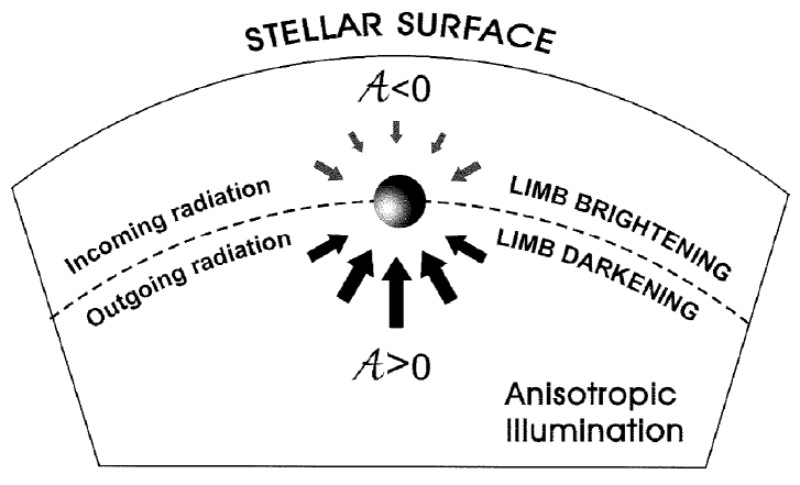
Figure 5.: The anisotropic illumination in a stellar atmosphere.

As an illustrative example, let us calculate the degree of anisotropy in an unmagnetized Milne–Eddington atmosphere (i.e. a medium in which the source function is $S\,=\,a\,+\,b\,\tau$, with $\tau$ the optical depth). Figure 4 shows, for various values of $b/a$, the variation with $\tau$ of the anisotropy factor

$${\cal{A}}\,=\,{{{\bar{J}}^{2}_{0}}\over{{\bar{J}}^{0}_{0}}},$$ (10)

where $\bar{J}^{0}_{0}$ and $\bar{J}^{2}_{0}$ are given by Eqs. (4) and (5), respectively. To obtain the results of Fig. 4 one has to solve the transfer equation in order to calculate the variation with $\mu={\rm cos}{\theta}$ of the Stokes $I$ parameter ($\theta$ is the angle between the ray direction and the $z$-axis of the reference system, which we choose here along the normal to the stellar surface). Note that ${\cal{A}}\,{\leq}\,0$ for the case of an atmosphere with no gradient in the source function (i.e. the curve with $b/a=0$ corresponding to $S=a$). The anisotropy factor (${\cal{A}}$) is essentially negative in atmospheres with very small $b/a$ values (see, for example, the curve with $b/a=0.1$), while ${\cal{A}}\,{\geq}\,0$ in atmospheres with sufficiently large $b/a$ ratios (see, for example, the curves with $b/a{\geq}1$). Note also that the larger $b/a$ the larger the anisotropy factor.

These results can be understood intuitively as follows. First, note that the tensor ${\bar{J}}^{2}_{0}$ (cf. Eq. 5) is dominated by the first term having the Stokes $I$ contribution. Therefore, predominantly vertical rays (i.e. those with $\mu>1/\sqrt{3}$) make positive contributions to $\bar{J}^{2}_{0}$, while predominantly horizontal rays (i.e. those with $\mu<1/\sqrt{3}$) make negative contributions. Second, as illustrated in Fig. 5, in a stellar atmosphere the outgoing intensities diminish with decreasing $\mu$ (i.e. they show limb darkening), while the incoming intensities augment with decreasing $\mu$ (i.e. they show limb brightening). In other words, in a stellar atmosphere the outgoing radiation is predominantly vertical, while the incoming radiation is predominantly horizontal. Thus, the outgoing intensities tend to produce positive contributions to $\bar{J}^{2}_{0}$, while the incoming intensities tend to produce negative contributions. Therefore, there is competition. It wins the subset of intensities (outgoing or incoming) having the largest variation with $\mu$. If $b/a=0$ the source function is constant ($S=a$) and the outgoing intensities have no $\mu$ dependence. This implies that ${\cal{A}}{\leq}0$ because the incoming intensities always show a dependence with $\mu$, even for a constant-property atmosphere. This is simply due to the presence of the stellar surface. However, as soon as $b/a$ becomes “large enough” the limb darkening of the outgoing intensities becomes more important than the limb brightening of the incoming intensities and the anisotropy factor ($\cal{A}$) becomes positive. It is straightforward to show that, for a given temperature gradient of the model atmosphere, the corresponding source function gradient is larger the bluer we go in the spectrum. This is the main reason why the anisotropy factor generally increases as we move in the spectrum from the IR toward the UV.

The anisotropy factor (cf. Eq. 10) is a fundamental quantity in scattering polarization. It is also of interest to note that its possible values are bounded as dictated by the following expression:

$$-{1\over{2\sqrt{2}}}\,\,{\leq}\,\,{\cal A}\,\,{\leq}\,\,{1\over{\sqrt{2}}}.$$ (11)

In the chosen reference frame (with the $z$-axis along the radial stellar direction), the largest $\cal{A}$ value corresponds to an illumination coming from purely vertical (radial) radiation beams and the lowest one to a purely horizontal radiation field.

The remaining radiation field tensors are more subtle, but their physical meaning can also be understood intuitively. The tensors $\bar{J}^{2}_{Q}$ (with $Q=1$ and $Q=2$) are complex quantities. They quantify the breaking of the axial symmetry of the Stokes $I$, $Q$ and $U$ parameters. If the physical properties of the stellar atmosphere model depend only on the radial direction, the ensuing $\bar{J}^{2}_{Q}$ tensors (with $Q=1$ and $Q=2$) are zero unless the magnetic field is inclined with respect to the radial direction. Figure 6 shows the variation with depth in a stellar model atmosphere of the real and imaginary parts of the $\bar{J}^{2}_{Q}$ tensors normalized to $\bar{J}^{0}_{0}$. Note that $\bar{J}^{K}_{Q}/\bar{J}^{0}_{0}\ll 1$, i.e. that the degree of “order” of the radiation field which interacts with the atoms of the stellar atmospheric model is weak. This must imply that the degree of “order” of the atomic system (i.e. the atomic polarization) has also to be weak. These considerations can suitably be taken into account in order to facilitate some analytical insight into and the numerical solution of the general equations.

Figure 6.: The tensors $\bar{J}^{2}_{Q}/\bar{J}^{0}_{0}$ corresponding to the self-consistent solution in the same stellar atmospheric model of Figure 2. The assumed horizontal magnetic field has $\Gamma=1$ and is orientated at $30^{\circ}$ with respect to the $x$-axis of Figure 1. The solid lines give the exact result. The dashed line of the panel for $\bar{J}^{2}_{0}/\bar{J}^{0}_{0}$ neglects the Stokes $Q$ contribution of Eq. (5). The dashed lines of the remaining panels neglect the contribution of the Stokes $I$ parameter to Eqs. (6) and (7). Therefore, the Stokes $I$ parameter is essential for calculating $\bar{J}^{2}_{0}$, while the Stokes $Q$ and $U$ parameters cannot be neglected (in general) when calculating $\bar{J}^{2}_{1}$ and $\bar{J}^{2}_{2}$.

The tensors $\bar{J}^{1}_{Q}$ are related to the circular polarization. Note that $\bar{J}^{1}_{Q}=0$ if the Stokes $V$ profile is perfectly antisymmetric, and that $\bar{J}^{1}_{1}=0$ if there is no azimuthal $\chi$ dependence in the Stokes $V$ parameter. We thus need to have net circular polarization in order to permit non-zero values for the $\bar{J}^{1}_{Q}$ tensors.

The most general situation in which all the above-mentioned radiation field tensors are non-zero is the case of a magnetized stellar atmosphere with macroscopic velocity gradients. In this article I will consider static stellar atmospheres for which the $\bar{J}^{1}_{Q}$ tensors can be assumed to be zero. As shown in Section 5, I will focus mainly on the generation of atomic alignment, which is directly related to the $\bar{J}^{2}_{Q}$ tensors and with the Hanle effect (i.e. with the modification of the linear polarization signals due to weak magnetic fields). In a future occasion I will address the issue of the generation of atomic orientation, which is intimately related to the $\bar{J}^{1}_{Q}$ tensors and with the modification of the circular polarization signals.

4. How to quantify the “order” of the atomic system?

The “order” of the atomic system (i.e. the atomic polarization) can be suitably quantified via the atomic density operator ($\rho^{\rm A}$) of quantum mechanics. This operator is represented in the basis $\{|{n}\rangle\}$ of energy eigenvectors via a matrix called the atomic density matrix whose elements are:

$$\rho^{A}_{ij}\,=\,\langle{i}|{\rho^{\rm A}}|{j}\rangle.$$ (12)

As clarified below, the diagonal elements (${{\rho}}^{A}_{ii}$) quantify the population of the state $|{i}\rangle$, while the non-diagonal elements (${{\rho}}^{A}_{ij}$, with $i\neq j$) quantify the degree of quantum interference (or coherence) between the states $|{i}\rangle$ and $|{j}\rangle$.

Let us give some information regarding the exact meaning of the atomic density matrix. First, note that the physical system under consideration is a volume element of a stellar atmosphere, which can be considered as being composed of three subsystems: the atoms (A) which emit, absorb, or scatter the radiation, the material perturbers (P) capable of influencing the excitation state of the atoms through inelastic and elastic collisions, and the radiation field (R) itself. The quantum-mechanical Hamiltonian operator ${\rm{\bf H}}$ of the whole system can be written, in the Schrödinger representation, in the form ${\rm{\bf H}={\bf H}_{0}+{\bf V}}$, where ${\rm{\bf H}_{0}}={\rm{\bf H}_{\rm A}}+{\rm{\bf H}_{\rm R}}+{\rm{\bf H}_{\rm P}}$ is the unperturbed Hamiltonian made up of the sum of the energies of the atoms, radiation and perturbers, while ${\rm{\bf V}}$ accounts for the various possible interactions among atoms, perturbers and radiation. Second, recall that there are two reasons which lead to the introduction of probabilities in the description of the state of a physical system such as that just defined. One is the quantum-mechanical uncertainty related to the measurement process. The other is due (as in classical statistical mechanics) to our lack of complete information on the initial state of the system. This means that its description cannot be given in terms of a pure state $|{\Psi}\rangle$, but through a statistical mixture of states (with the probability $p_{k}$ of finding the system in the state vector $|{\Psi}_{k}\rangle$). To incorporate into the quantum mechanical formalism the incomplete information we posses about the state of the system, the mixed state density operator (i.e. ${{\rho}}=\sum_{k}{p}_{k}|{\Psi}_{k}\rangle\langle\Psi_{k}|$) was introduced (von Neumann, 1927; but see Fano, 1957). The essential point is that the microscopic interactions of our atomic subsystem with the perturbers and the radiation field drive the atomic subsystem into a mixed state which can be described by the density operator but not by a pure state.

To grasp the usefulness of the atomic density operator, consider a complete set $\{|{n}\rangle\}$ of eigenvectors of the atomic Hamiltonian (i.e. ${\bf H}_{A}|{n}\rangle=E_{n}|{n}\rangle$, with $E_{{}_{n}}$ the energy eigenvalue corresponding to $|{n}\rangle$). To be able to make physical predictions about measurements bearing only on the atomic subsystem (A), the density operator ${{\rho}}^{A}$ of this subsystem is introduced (i.e. ${{\rho}}^{A}$ = Tr_P (Tr${}_{\rm R}{{\rho}})$, where the symbols Tr_P and Tr_R mean the traces over the perturbers (P) and the radiation field (R) coordinates respectively; note that the trace of a matrix is the sum of its diagonal elements). Calculating the matrix elements ${{\rho}}_{ij}^{A}$ of ${{\rho}}^{A}$ in the set $\{|{n}\rangle\}$ one finds:

• ${{\rho}}^{A}_{ii}$ represents the average probability of finding the system in the state $|{i}\rangle$ (which implies that ${{\rho}}^{A}_{ii}$ quantifies the population of the state $|{i}\rangle$).

• ${{\rho}}^{A}_{ij}$ (with $i\neq j$) gives account of the interference effects between the states $|{i}\rangle$ and $|{j}\rangle$, which can appear simply because each state $|{\Psi}_{k}>$ of the statistical mixture is (in general) given by a coherent linear superposition of the states $\{|{n}\rangle\}$. As mentioned above, the non-diagonal elements of ${\rho}^{A}$ are called coherences.

The density operator ${{\rho}}$ of the total system (atoms, perturbers and radiation) contains all physically significant information on the system. In fact, the expectation value of any observable, described in the Schrödinger picture by a Hermitian operator $\bf O$, is given by (cf. Fano, 1957):

$$\langle{\bf O}\rangle(t)={\rm Tr}({\rho}{\bf O})={\rm Tr}({\rho}_{I}{\bf O}_{I}),$$ (13)

where ${\bf O}_{I}$ and ${\rho}_{I}$ are the corresponding operators in the interaction (or Heisenberg) picture of quantum mechanics (see any suitable advanced textbook). As indicated by this expression, the expectation value of an observable has the same structural form in the two quantum mechanical approaches (i.e. in the Schrödinger and in the Heisenberg representations). However, the Heisenberg picture has the advantage of forcing the time dependence of wave functions to arise solely from the effect of the perturbing Hamiltonian ${\rm{\bf V}}$, thus facilitating a perturbation approach.

Equation (13) is one of the two basic equations on which the density-matrix polarization transfer theory is based. The other fundamental equation is the equation of motion for the density operator ${\rho}_{I}$, which reads

$$i{h\over{2\pi}}{{\partial{{\rho}_{I}}}\over{{\partial{t}}}}=[{\rm{\bf V}_{I}},{\rho}_{I}].$$ (14)

The combination of Eqs. (13) and (14) leads to an exact equation for $d\langle{\bf O}\rangle/dt$, which can be used to derive the time evolution of physical quantities (e.g. the time evolution of the diagonal and non-diagonal elements of the atomic density matrix ${{\rho}}^{A}$ due to the coupling of the atomic system A with the radiation field R considered as a reservoir; cf. Cohen-Tannoudji, 1977). As reviewed in more detail by Trujillo Bueno (1990), the above-mentioned exact equation for the time evolution of the observables is the starting point in Landi Degl’Innocenti’s (1983) QED derivation of the statistical equilibrium and Stokes-vector transfer equations.

Finally, we should mention that there are two relevant representations of the atomic density operator: the standard (already introduced above) and the spherical statistical tensor representation (Omont, 1977; Blum, 1981). Let us introduce them in terms of the basis of eigenvectors of the angular momentum ($|{\alpha}JM>$, with $\alpha$ indicating the quantum numbers of a given term—e.g. $\alpha=nLS$ if the atom is described by the $L-S$ coupling scheme).

In the standard representation the coherences between magnetic sublevels pertaining to the same $J$-level are given by:

$$\rho^{\rm A}_{\alpha{J}}(M,M^{{}^{\prime}})\,=\,\langle{\alpha}JM|{\rho^{\rm A}}|{\alpha}JM^{{}^{\prime}}\rangle,$$ (15)

while the total population of the $J$-level is

$$n_{J}=\sum_{M}\,{\rho^{\rm A}_{\alpha{J}}}(M,M),$$ (16)

where $\rho^{\rm A}_{\alpha{J}}(M,M)$ is the population of the sublevel with magnetic quantum number $M$.

In the spherical statistical tensor representation the density-matrix elements are denoted by the symbol $\rho^{K}_{Q}$ (with $K=0,...,2J$ and $-K{\leq}Q{\leq}K$). The $\rho^{K}_{Q}$ elements are given by the following linear combinations of the density-matrix elements of the standard representation (cf. Omont, 1977):

$${\rho^{K}_{Q}}({\alpha}J)=\sum_{MM^{\prime}}(-1)^{J-M}{\sqrt{2K+1}}\left(\begin{array}[]{ccc}J&J&K\\ M&-M^{{}^{\prime}}&-Q\end{array}\right){\rho^{\rm A}_{{\alpha}J}}(M,M^{{}^{\prime}}),$$ (17)

where the 3-j symbol is defined as indicated by any suitable textbook on quantum mechanics.

For instance, for a level with total angular momentum $J=1$

$$\rho^{0}_{0}={1\over{\sqrt{3}}}[\rho^{\rm A}_{1}(1,1)+\rho^{\rm A}_{1}(0,0)+\rho^{\rm A}_{1}(-1,-1)]={1\over{\sqrt{3}}}\,n_{J=1},$$ (18)

$$\rho^{1}_{0}={1\over{\sqrt{2}}}[\rho^{\rm A}_{1}(1,1)-\rho^{\rm A}_{1}(-1,-1)],$$ (19)

$$\rho^{1}_{1}=-{1\over{\sqrt{2}}}[\rho^{\rm A}_{1}(1,0)+\rho^{\rm A}_{1}(0,-1)],$$ (20)

$$\rho^{2}_{0}={1\over{\sqrt{6}}}[\rho^{\rm A}_{1}(1,1)-2\rho^{\rm A}_{1}(0,0)+\rho^{\rm A}_{1}(-1,-1)],$$ (21)

$$\rho^{2}_{1}=-{1\over{\sqrt{2}}}[\rho^{\rm A}_{1}(1,0)-\rho^{\rm A}_{1}(0,-1)],$$ (22)

$$\rho^{2}_{2}=\rho^{\rm A}_{1}(1,-1).$$ (23)

Note that the $\rho^{K}_{Q}$ elements with $Q=0$ are real numbers given by linear combinations of the populations of the various Zeeman sublevels corresponding to the level of total angular momentum $J$. The total population of the atomic level is quantified by ${\sqrt{2J+1}}{\rho^{0}_{0}}$, while the population imbalances among such Zeeman sublevels are quantified by $\rho^{1}_{0}$ (i.e. by the $Q=0$ orientation coefficient) and by $\rho^{2}_{0}$ (i.e. by the $Q=0$ alignment coefficient). However, the $\rho^{K}_{Q}$ elements with $Q{\neq}0$ are complex numbers given by linear combinations of the coherences between Zeeman sublevels whose magnetic quantum numbers differ by $Q$. In fact, since the density operator is Hermitian, we have that for each spherical statistical tensor component $\rho^{K}_{Q}$ with $Q>0$, there exists another component with $Q<0$ given by $\rho^{K}_{-Q}=(-1)^{Q}[\rho^{K}_{Q}]^{*}$. We thus have $(2J+1)^{2}$ density-matrix elements corresponding to each level of total angular momentum $J$ (both in the standard and spherical tensor representations).

Both formalisms are totally equivalent. However, in the context of scattering polarization and the Hanle effect, it is more convenient to work within the framework of the spherical statistical tensor representation due to the following reasons (cf. Landi Degl’Innocenti 1982). The first advantage is directly related to the fact that the density matrix elements on the basis of the eigenvectors of the angular momentum depend on the reference system chosen to define such eigenvectors. It turns out that the spherical statistical tensors defined by Eq. (17) have simpler transformation laws with respect to rotations of the coordinate system: their transformation law involves just one rotation matrix instead of the product of two rotation matrices. The second advantage is that the $\rho^{K}_{Q}$ elements themselves provide the most suitable way of quantifying, at the atomic level, the information that we need to be able to calculate all the “sources” and “sinks” of linear and circular polarization within the medium under consideration (i.e. they have a clear physical interpretation). For instance, if $\rho^{2}_{0}(J_{u}){\neq}0$ and $\rho^{1}_{0}(J_{u}){\neq}0$ we have local sources of linear and circular polarization, respectively, even in the absence of magnetic fields. In the Hanle effect regimes considered in this article the width of the spectral line is much larger than the Zeeman splitting and the Stokes $Q$ and $U$ components of the line emission vector are given by:

$${\epsilon}_{Q}={\epsilon_{0}}\,w^{(2)}_{J_{u}J_{l}}\Big{\{}\frac{3}{2\sqrt{2}}(\mu^{2}-1){\rho}^{2}_{0}-\sqrt{3}\mu\sqrt{1-\mu^{2}}(\cos\chi{\rm Re}[{{\rho}}^{2}_{1}]-\sin\chi{\rm Im}[{{\rho}}^{2}_{1}])$$

$$\hskip 137.31255pt-\frac{\sqrt{3}}{2}(1+\mu^{2})(\cos 2\chi\,{\rm Re}[{{\rho}}^{2}_{2}]-\sin 2\chi\,{\rm Im}[{{\rho}}^{2}_{2}])\Big{\}},$$ (24)

$$\epsilon_{U}={\epsilon_{0}}\,w^{(2)}_{J_{u}J_{l}}\sqrt{3}\,\Big{\{}\sqrt{1-\mu^{2}}(\sin\chi{\rm Re}[{{\rho}}^{2}_{1}]+\cos\chi{\rm Im}[{{\rho}}^{2}_{1}])$$

$$\hskip 93.95122pt+\mu(\sin 2\chi\,{\rm Re}[{{\rho}}^{2}_{2}]+\cos 2\chi\,{\rm Im}[{{\rho}}^{2}_{2}])\Big{\}},$$ (25)

where the $\rho^{K}_{Q}$ values are those of the upper level of the line transition under consideration, $\epsilon_{0}=(h\nu/4\pi)A_{ul}{\phi_{x}}{\cal N}\sqrt{2J_{u}+1}$ (with $\cal N$ the total number of atoms per unit volume), $w^{(2)}_{J_{u}J_{l}}$ is the symbol introduced by Landi Degl’Innocenti (1984) (which depends only on $J_{u}$ and $J_{l}$), and where the orientation of the ray is specified by $\mu={\rm cos}\theta$ (with $\theta$ the polar angle) and by the azimuthal angle $\chi$. The elements $\eta_{Q}$ and $\eta_{U}$ of the absorption matrix are given by identical expressions (i.e. by $\eta_{Q}=\epsilon_{Q}$ and by $\eta_{U}=\epsilon_{U}$), but with $\eta_{0}=(h\nu/4\pi)B_{lu}{\phi_{x}}{\cal N}\sqrt{2J_{l}+1}$ instead of $\epsilon_{0}$, $w^{(2)}_{J_{l}J_{u}}$ instead of $w^{(2)}_{J_{u}J_{l}}$ and with the $\rho^{K}_{Q}$ values of the lower level of the line transition (instead of those of the upper level). Note that $\epsilon_{Q}$ and $\eta_{Q}$ depend on both the population imbalances ($\rho^{2}_{0}$) and on the coherences ($\rho^{2}_{Q}$, with $Q=1,2$), while $\epsilon_{U}$ and $\eta_{U}$ depend only on the coherences. Recall also that the emission vector and the absorption matrix are the two fundamental quantities which appear in the Stokes-vector transfer equation.

Finally, an additional reason for the suitability of the spherical tensor representation is that the limiting case in which polarization phenomena are neglected (cf. Mihalas, 1978) can be obtained simply by retaining only the terms with $K=Q=0$.

5. Transfer of “order” from the radiation field to the atomic system

There are two mechanisms which can lead to transfer of “order” from the radiation field to the atomic system: upper-level selective population pumping and lower-level selective depopulation pumping. The requirements are that the pumping light must be necessarily anisotropic, and/or polarized and/or to have spectral structure over a frequency interval $\Delta\nu$ smaller than the frequency separation between the Zeeman sublevels.

Upper-level population pumping occurs when some upper-state sublevels have more chances of being populated than others. For instance, if an unpolarized light beam propagating along the direction chosen as the quantization axis illuminates a gas of two level atoms with $J_{l}=0$ and $J_{u}=1$, only the transitions corresponding to ${\Delta}M={\pm}1$ are effective, so that no transitions occur to the $M=0$ sublevel of the upper level. Thus, in the absence of any relaxation mechanisms, the upper-level sublevels with $M=1$ and $M=-1$ would be more populated than the $M=0$ sublevel and the fractional upper-level alignment coefficient $\sigma^{2}_{0}(u)={\rho}^{2}_{0}(u)/{\rho}^{0}_{0}(u)=1/{\sqrt{2}}$.

Lower-level depopulation pumping occurs when some lower-state sublevels absorb light more strongly than others. As a result an excess population tends to build up in the weakly absorbing sublevels. For instance, if an unpolarized light beam propagating along the direction chosen as the quantization axis illuminates a gas of two level atoms with $J_{l}=1$ and $J_{u}=0$, only the transitions corresponding to ${\Delta}M={\pm}1$ are effective, so that no transitions can occur out of the $M=0$ sublevel of the lower level. On the other hand, the spontaneous de-excitation from the upper level populates with equal probability the three sublevels ($M=-1,0,+1$) of the lower level. In the absence of any relaxation mechanisms, the final result of this optical-pumping cycle is that all atoms will eventually be pumped into the $M=0$ sublevel of the lower level, and the medium will become transparent (Happer, 1972). Under such ideal laboratory conditions (illumination by a unidirectional light beam and absence of depolarizing mechanisms) the fractional lower-level alignment coefficient is $\sigma^{2}_{0}(l)={\rho}^{2}_{0}(l)/{\rho}^{0}_{0}(l)=-{\sqrt{2}}$, i.e. a factor 2 larger (in absolute value) than the fractional upper-level alignment corresponding to the previous triplet-line case.

The Nobel laureate Alfred Kastler (1950) was actually the first scientist to propose that optical pumping under laboratory conditions can be used as a method to change the relative populations of Zeeman sublevels and of hyperfine levels of the ground state of atoms. What we have been emphasizing over the last few years is that the very same mechanism (lower-level depopulation pumping) is operating in the atmospheres of the stars, and that it constitutes an essential physical ingredient for understanding the second solar spectrum.

Lower-level depopulation pumping in solar-like atmospheres was investigated in detail by Trujillo Bueno and Landi Degl’Innocenti (1997) including depolarizing collisions and radiative transfer effects. We chose that particular type of line transition (i.e. $1\,\rightarrow\,0\,\rightarrow\,1$) to point out clearly that lower-level depopulation pumping due to the anisotropy of the solar radiation field can lead to sizeable amounts of ground-level atomic polarization and to emergent linear polarization signals with amplitudes in the observable range. Soon afterwards, Landi Degl’Innocenti (1998) succeeded in deriving analytical expressions for the Stokes-$Q$ component of the emission vector and of the absorption matrix corresponding to the D₁ and D₂ lines of Na I, and could show by adjusting free parameters that a certain amount of atomic polarization in the hyperfine components of the ground level of sodium leads to a remarkably good fit of the complex fractional linear polarization pattern observed by Stenflo and Keller (1997), including the “enigmatic” line-centre peaks. A subsequent theoretical investigation (Trujillo Bueno 1999) was aimed at demonstrating that depopulation pumping in the solar atmosphere (and the induced lower-level atomic polarization) can actually produce similar amounts of linear polarization for some groups of line transitions (having different $J_{l}$ and $J_{u}$ values) for which the simplified resonance line polarization theory (which neglects the influence of lower-level depopulation pumping) predicts drastically different emergent polarizations. Based on this result, I suggested a possible explanation of the “enigmatic” linear polarization amplitudes observed by Stenflo et al. (1983, 2000) in the Mg I $b$ lines (see Trujillo Bueno 1999; Sections 6 and 7). That theoretical investigation demonstrated that the presence of a sizeable amount of atomic polarization in the metastable lower-levels of the Mg $b_{1}$ and $b_{2}$ lines would explain in a natural way the similar polarization amplitudes observed in the Mg $b$ lines (and also those observed in the three lines of multiplet No. 3 of Ca I, which is also a ${}^{3}{\rm P}^{0}\,-\,^{3}{\rm S}$ multiplet). This result for the Mg $b$ lines was particularly encouraging because, contrary to the case of the sodium D-lines, it is totally impossible to argue that there might perhaps exist an alternative explanation of the observed polarization peaks based on a multilevel scenario characterized by the absence of lower-level polarization (see Trujillo Bueno 1999; Sections 5 and 6).

In addition to the two previous pumping mechanisms, which allow the direct transfer of “order” from the radiation field to the atomic system, there is an additional pumping process which also comes into play: repopulation pumping. This pumping occurs either when the lower-level is repopulated as a result of spontaneous decay of a polarized upper level or when the upper-level is repopulated as a result of absorptions of a polarized lower level. As can be intuitively expected, the repopulation pumping rates are proportional to the atomic polarization of the atomic levels.

5.1. The two-level atom in the absence of magnetic fields

The best thing we can do to facilitate understanding of all these pumping mechanisms is to show them in action for a particularly illuminating example: the scattering line polarization problem in a one-dimensional unmagnetized stellar atmosphere formed by a gas of two level atoms with $J_{l}=J_{u}=1$ (cf. Trujillo Bueno 1999). For this case, the only non-zero radiation field tensors are $\bar{J}^{0}_{0}$ and $\bar{J}^{2}_{0}$ and the unknowns of the problem at each spatial point are simply $\rho^{0}_{0}(l)$, $\rho^{2}_{0}(l)$, $\rho^{0}_{0}(u)$ and $\rho^{2}_{0}(u)$. The rate equations which govern the temporal evolution of the alignment coefficients ($\rho^{2}_{0}$) of the upper and lower levels can be deduced applying the density matrix polarization transfer theory of Landi Degl’Innocenti (1983). We obtain:

$${{d}\over{d\,t}}\,{{\rho}^{2}_{0}(u)}\,=\,-\left[{B_{lu}\over 2}{{{\bar{J}}^{2}_{0}}}{{{\rho}^{0}_{0}}(l)}+{{B_{lu}}\over{{2}}}{{{\bar{J}}^{0}_{0}}}{{{\rho}^{2}_{0}}(l)}+{B_{lu}\over{\sqrt{2}}}{{{\bar{J}}^{2}_{0}}}{{{\rho}^{2}_{0}}(l)}\right]-A_{ul}\,{{{\rho}^{2}_{0}}(u)}$$ (26)

$$+C^{(2)}_{lu}{{{\rho}^{2}_{0}}(l)}-(C_{ul}+D_{u}){{{\rho}^{2}_{0}}(u)},$$

$${{d}\over{d\,t}}\,{{\rho}^{2}_{0}(l)}\,=\,-A_{ul}{{{\rho}^{2}_{0}}(u)}+\left[{B_{lu}}{{{\bar{J}}^{2}_{0}}}{{{\rho}^{0}_{0}}(l)}-2{{B_{lu}}}{{{\bar{J}}^{0}_{0}}}{{{\rho}^{2}_{0}}(l)}-{B_{lu}\over{\sqrt{2}}}{{{\bar{J}}^{2}_{0}}}{{{\rho}^{2}_{0}}(l)}\right]$$ (27)

$$+2C_{ul}{{{\rho}^{2}_{0}}(u)}-2(C_{lu}+D_{l}){{{\rho}^{2}_{0}}(l)}.$$

These equations have contributions coming from transfer and relaxation rates due to radiative and collisional terms. I have neglected the stimulated emission terms. Assuming statistical equilibrium (i.e. ${\rm d}{\rho^{K}_{Q}}/{\rm d}t=0$), neglecting also inelastic collisions (i.e. the $C_{lu}$ and $C_{ul}$ terms) and the terms containing the products ${{{\bar{J}}^{2}_{0}}}{{{\rho}^{2}_{0}}}$ (because in a weakly polarizing medium like the solar atmosphere ${\bar{J}}^{2}_{0}/{\bar{J}}^{0}_{0}\ll 1$ and ${\rho}^{2}_{0}/{\rho}^{0}_{0}\ll 1$) we find:

$${{{\rho^{2}_{0}}({\rm up})}}\,{\approx}\,{{-1}\over{2\,(1+{{\delta}_{u}})}}\,\left[{{B_{lu}{\bar{J}^{2}_{0}}}\over{A_{ul}}}\,{{{\rho^{0}_{0}}({\rm low})}}+{{B_{lu}{\bar{J}^{0}_{0}}}\over{A_{ul}}}\,{{{\rho^{2}_{0}}({\rm low})}}\right],$$ (28)

$${{{\rho^{2}_{0}}({\rm low})}}\,{\approx}\,\,{1\over{2\,(1+{{\delta}_{l}})}}\,\left[{{B_{lu}{\bar{J}^{2}_{0}}}\over{B_{lu}{\bar{J}^{0}_{0}}}}\,{{{\rho^{0}_{0}}({\rm low})}}-{{A_{ul}}\over{B_{lu}{\bar{J}^{0}_{0}}}}\,{{{\rho^{2}_{0}}({\rm up})}}\right],$$ (29)

where ${\delta}_{u}=D_{u}/A_{ul}$ and ${\delta}_{l}=D_{l}/{B_{lu}{\bar{J}^{0}_{0}}}$, with $D_{u}$ and $D_{l}$ the depolarizing rates due to elastic collisions.

The first term within the brackets of Eq. (28) is due to the upper-level population pumping mechanism, while the first term within the brackets of Eq. (29) is due to the lower-level depopulation pumping mechanism. Both are given by the rate $B_{lu}{\bar{J}^{2}_{0}}{\rho^{0}_{0}}({\rm low})$; the only difference is that the upper-level pumping contribution is multiplied by the lifetime of the upper level (i.e. by $1/A_{ul}$), while the lower-level pumping contribution is multiplied by the lifetime of the ground level (i.e. by $1/B_{lu}{\bar{J}^{0}_{0}}$, which for optical line transitions in solar-like atmospheres is about two orders of magnitude larger than the upper-level lifetime).

The second term within the brackets of Eq. (29) is due to the repopulation pumping resulting from the spontaneous decay of the polarized upper level, while the second term within the brackets of Eq. (28) is due to the repopulation pumping resulting from the absorption process from the polarized lower level.

The previous two equations have been useful in identifying the contributions corresponding to the various pumping mechanisms. However, the relevant quantities of interest to understanding the observed polarization amplitudes are the fractional atomic polarization ($\sigma^{2}_{0}=\rho^{2}_{0}/\rho^{0}_{0}$) of each level. In fact, the emergent fractional linear polarization close to the solar limb is approximately given by:

$${Q\over{I}}\,\approx\,{\cal W}\,\sigma^{2}_{0}({\rm up})\,-\,{\cal Z}\,\sigma^{2}_{0}({\rm low}),$$ (30)

where ${\cal W}$ and ${\cal Z}$ are simply numbers given by the total angular momentum values of the lower and upper atomic levels of the line transition under consideration. In this formula the $\sigma^{2}_{0}$ values have to be calculated at the spatial point (situated along the line of sight) where the optical depth is unity. This formula (see Trujillo Bueno 1999) may be considered as the generalization of the Eddington–Barbier relation to the non-magnetic scattering polarization case. (Note that I have rewritten it here in a way such that the positive reference-direction for the Stokes $Q$ parameter is now chosen along the line perpendicular to the radial direction through the observed point, and not along the radial direction as it was chosen in the above-mentioned paper and in Eqs. 24 and 25.)

The equations for $\sigma^{2}_{0}({\rm up})$ and $\sigma^{2}_{0}({\rm low})$ can be obtained easily after dividing Eqs. (28) and (29) by $\rho^{0}_{0}(l)$ and taking into account that $\rho^{0}_{0}(u)/\rho^{0}_{0}(l)\,\approx\,B_{lu}{\bar{J}^{0}_{0}}/A_{ul}$. (Note that this is a good approximation for a weakly anisotropic medium in which the inelastic collisional rates have been assumed to be much smaller than the radiative rates.) The result reads:

$${{\sigma^{2}_{0}({\rm up})}}\,{\approx}\,{{-1}\over{2\,(1+{\delta_{u}})}}\,\left[{{{\bar{J}^{2}_{0}}}\over{{\bar{J}^{0}_{0}}}}+{{\sigma^{2}_{0}({\rm low})}}\right],$$ (31)

$${{\sigma^{2}_{0}({\rm low})}}\,{\approx}\,{1\over{2\,(1+{\delta_{l}})}}\,\left[{{{\bar{J}^{2}_{0}}}\over{{\bar{J}^{0}_{0}}}}-{{\sigma^{2}_{0}({\rm up})}}\right].$$ (32)

We thus see that there exists a fascinating closed loop connecting the lower-level and upper-level polarizations. The atomic polarization of the upper level produced by the anisotropic illumination of the atoms is modified (typically enhanced!) because of the atomic polarization of the lower level, and vice versa. The only way to frustrate this remarkable communication between the two levels is by forcing one of the two levels to be totally unpolarized, which can only occur in practice if either $\delta_{u}$ or $\delta_{l}$ turns out to be very much larger than unity. In fact, if we assume that the atomic polarization of the lower level is totally destroyed by elastic collisions (i.e. $\delta_{l}\,\rightarrow\,\infty$) and that the upper level is insensitive to such collisions (i.e. $\delta_{u}=0$) we find ${\sigma^{2}_{0}({\rm up})}\,\approx\,-0.5\,({\bar{J}^{2}_{0}}/{\bar{J}^{0}_{0}})$, in agreement with the self-consistent numerical results given by the dashed lines of Fig. 1 of Trujillo Bueno (1999). However, if we assume that both atomic levels are insensitive to elastic collisions (i.e. that $\delta_{l}=\delta_{u}=0$), we then find ${\sigma^{2}_{0}({\rm up})}\,\approx\,-{\sigma^{2}_{0}({\rm low})}\,\approx\,-\,{\bar{J}^{2}_{0}}/{\bar{J}^{0}_{0}}$, in agreement with the self-consistent numerical result given in Fig. 3 of Trujillo Bueno (1999).

5.2. The two-level atom in the presence of weak magnetic fields

What do we obtain for the atomic polarization of the ground and excited levels of a $1{\rightarrow}1$ transition if we include the effect of a weak magnetic field? Obviously, the situation becomes more complicated. First, the number of unknowns at each spatial point is 12 instead of just four. The density matrix elements whose values are sought are: $\rho^{0}_{0}(l)$, $\rho^{2}_{0}(l)$, the real and imaginary parts of $\rho^{2}_{1}(l)$ and of $\rho^{2}_{2}(l)$, $\rho^{0}_{0}(u)$, $\rho^{2}_{0}(u)$ and the real and imaginary parts of $\rho^{2}_{1}(u)$ and of $\rho^{2}_{2}(u)$. Second, there are two “natural” choices for the direction of the $z$-axis of the reference system used to formulate the rate equations: ($a$) the magnetic field reference frame in which the $z$-axis is aligned with the local magnetic field direction and ($b$) the stellar radial direction itself. For developing a general multilevel scattering polarization and Hanle-effect code we prefer option $b$ (which is in fact the choice in Sections 6 and 7). However, as done in the remaining part of this section, it is convenient to formulate the rate equations in the magnetic field reference frame if the interest lies in achieving some analytical insight.

The two following expressions are a particular case of the equations derived by Landi Degl’Innocenti (1985). They are valid for a $1{\rightarrow}1$ transition of a two-level atom in a weakly anisotropic and magnetized stellar atmosphere in which the effect of collisions is assumed to be negligible:

$${\sigma^{K}_{Q}}({u})={\rho^{K}_{Q}}(u)/{\rho^{0}_{0}}(u)=-{{{1\over{2}}(1+i{\Gamma_{l}}Q)\,+\,{1\over{4}}}\over{(1+i{\Gamma_{u}}Q)(1+i{\Gamma_{l}}Q)\,-\,{1\over{4}}}}\,\,(-1)^{Q}\,{{\bar{J}^{K}_{-Q}}\over{\bar{J}^{0}_{0}}},$$ (33)

$${\sigma^{K}_{Q}}({l})={\rho^{K}_{Q}}(l)/{\rho^{0}_{0}}(l)=(-1)^{K}{{{1\over{2}}(1+i{\Gamma_{u}}Q)\,+\,{1\over{4}}}\over{(1+i{\Gamma_{u}}Q)(1+i{\Gamma_{l}}Q)\,-\,{1\over{4}}}}\,\,(-1)^{Q}\,{{\bar{J}^{K}_{-Q}}\over{\bar{J}^{0}_{0}}}.$$ (34)

These formulae are valid for $K=1$ and $K=2$. They show that, once the fractional radiation field tensors (i.e. ${{\bar{J}^{K}_{-Q}}/{\bar{J}^{0}_{0}}}$) are known in the magnetic field reference frame, the fractional atomic polarization of each level depend only on the dimensionless quantities $\Gamma_{u}$ and $\Gamma_{l}$, which are given by:

$$\Gamma_{u}=8.79\times 10^{6}{\rm B}g_{J_{u}}/A_{ul},$$ (35)

$$\Gamma_{l}=8.79\times 10^{6}{\rm B}g_{J_{l}}/B_{lu}\bar{J}^{0}_{0}.$$ (36)

The previous equations for ${\sigma^{K}_{Q}}({u})$ and ${\sigma^{K}_{Q}}({l})$ show that in the magnetic field reference frame the population imbalances (i.e. ${\sigma^{K}_{0}}$) are insensitive to the magnetic field, while the coherences (i.e. ${\sigma^{K}_{Q}}$ with $Q{\neq}0$) are reduced and dephased as the magnetic field is increased. Finally, note that magnetic fields such that $\Gamma_{l}\,\approx\,1$ are very efficient in depolarizing the ground level, which has a significant feedback on the upper-level coherences, while fields such that $\Gamma_{u}\,\approx\,1$ are very efficient in depolarizing the excited level.

Some polarization diagrams illustrating the lower-level and upper-level Hanle effects for single scattering events in two-level atomic models have been presented by Landolfi & Landi Degl’Innocenti (1986). Similar type of Hanle-effect diagrams, but taking into account radiative transfer effects in isothermal stellar atmospheres, will be published by Manso Sainz & Trujillo Bueno (2001b).

6. Multilevel scattering polarization

The theoretical interpretation of scattering polarization signals requires a calculation of the the atomic polarization considering complex atomic and molecular systems. This is a very involved non-linear and non-local problem which has been solved with sufficient generality only recently (see below). It consists in calculating, at each spatial grid-point of the assumed astrophysical plasma, the density-matrix elements which are consistent with the properties of the polarized radiation field generated within the medium.

From multilevel radiative transfer simulations without polarization physics we know that the two-level atom model is, with few exceptions, an unsuitable approximation for modeling the Fraunhofer spectrum. Obviously, the same statement should be applied (but with much more emphasis) to the realm of the second solar spectrum, which is due to coherence transfer effects. In order to exploit its rich diagnostic potential (e.g. with the aim of exploring magnetoturbulence and/or to improve our understanding of chromospheric magnetism) it is crucial to investigate the generation and transfer of atomic polarization considering realistic multilevel models and taking fully into account all the above-mentioned pumping mechanisms in the presence (and absence) of the Hanle effect induced by weak magnetic fields (e.g. from 1 milligauss to 100 gauss). During the last year Rafael Manso Sainz and I have successfully developed a general multilevel scattering polarization radiative transfer code, which is currently allowing us to carry out this type of investigations via realistic numerical simulations. Our multilevel scattering polarization code solves the following set of equations:

(a) The rate equations giving the time evolution of the atomic density matrix elements. In these equations the radiative rates are given in terms of the radiation field tensors introduced in Section 3. For the moment we assume statistical equilibrium (SE) (i.e. $d{\rho^{K}_{Q}}/dt=0$).

(b) The Stokes-vector transfer equations where the components of the emission vector and those of the absorption matrix depend on the density-matrix elements themselves. For the moment, we assume one-dimensional (1D) plane-parallel geometry, but we have also developed suitable formal solution methods for considering spherical circumstellar envelopes and realistic 3D model atmospheres with horizontal inhomogeneities.

These SE and RT equations were derived from the principles of quantum electrodynamics by Landi Degl’Innocenti (1983). This density-matrix polarization transfer theory is based on the Markovian assumption of complete frequency redistribution (see a critical review of this CRD polarization transfer theory in Trujillo Bueno 1990). For problems where the only significant coherences are those between the sublevels of degenerate levels, this CRD theory should provide a physically consistent description of scattering phenomena if the spectrum of the pumping radiation is flat across a frequency range wider than the inverse lifetime of the levels (Landi Degl’Innocenti et al. 1997). As we shall see below, this seems to be a sufficiently good approximation for modeling the observed polarization in a number of spectral lines of diagnostic interest (e.g. the Ca ii IR triplet and the Mg $b$ lines).

Other scientists (e.g. Bommier and Sahal-Bréchot 1978) had previously formulated the statistical equilibrium equations for the Hanle effect regime applying also the theory of the master equation of a “small system” (the atom) interacting with a “big reservoir” (the radiation field) (cf. Cohen-Tannoudji 1977; Cohen-Tannoudji et al. 1992). The interest of Landi’s theoretical work stems from the fact that he was able to achieve a general unified theoretical derivation of both, the statistical equilibrium equations and the radiative transfer equations. From the point of view of numerical radiative transfer our coherency transfer code is based on the fast iterative methods which the author of this article developed for multilevel scattering polarization and Hanle effect applications (see Trujillo Bueno 1999; and note that the two-level atom scattering polarization problem with lower-level depopulation pumping solved in that paper is also a non-linear and non-local problem of the same nature as the general multilevel case considered here).

6.1. Three-level systems and the “enigmatic” Ca ii 8662 Å  line

The quest to understand the physical origin of the second solar spectrum will be facilitated if we first gain some physical insight on how the various pumping mechanisms leads to atomic polarization in three-level atomic systems under stellar atmospheric conditions.

There are a number of schematic three-state configurations which our laser physics colleagues like to include in their textbooks: cascade, vee (${\bf{V}}$) and lambda (${\bf{\Lambda}}$). The linkage pattern is $1\,\leftrightarrow\,2\leftrightarrow\,3$ for any ranking of the relative energy values. Thus, the cascade configuration is the one in which the energies increase with index $i$, $E_{1}\,<\,E_{2}\,<\,E_{3}$. The vee configuration occurs when the central state (i.e. level 2) lies lowest in energy. A third possibility, the lambda configuration, occurs when the central state lies highest in energy.

Unfortunately, I do not have enough space here to present and discuss the results of our coherency transfer calculations in stellar atmospheric models for all these three-level systems. I have to make a choice: the lambda configuration with $J_{1}=1/2$, $J_{2}=1/2$, and $J_{3}=3/2$. My motivation behind this choice is two-fold. First, it is precisely the configuration of the Raman scattering process, in which a photon of one frequency is absorbed and a second frequency may be re-emitted. Second, this particular three-level atomic system will help to understand physically our successful modeling of the “enigmatic” fractional linear polarization observed by Stenflo et al. (2000) in the Ca ii IR triplet (see Manso Sainz and Trujillo Bueno 2001a). To this end, the atomic parameters of the $1\,\leftrightarrow\,2$ transition have been chosen to be identical to that of the H line of Ca ii, while those of the $2\,\leftrightarrow\,3$ transition correspond to that of the 8662 Å  line of the Ca ii IR triplet. The observations were considered “enigmatic” especially because this 8662 Å  line should be, according to Stenflo et al. (2000), intrinsically unpolarizable. However, their observations show a polarized peak (see also Dittmann et al. 2001). They considered this line “intrinsically unpolarizable” because its upper level (and also the lower level of the H-line) cannot harbour any atomic alignment (because $J_{2}=1/2$ and calcium has no hyperfine structure).

Figure 7.: Left: The fractional atomic polarization of the lower level of the 8662 Å  line versus its optical depth (see the thin solid line yielding a surface value of $-3\%$). The thick solid line yielding a surface value of $-7\%$ shows $-{\bar{J}^{2}_{0}}/{\bar{J}^{0}_{0}}$. Right: The corresponding emergent fractional linear polarization of the 8662 Å  line at $\mu=0.1$.

Figure 7 shows the self-consistent results for the unmagnetized case. The thin line of the left panel gives the variation with line optical depth of the fractional atomic polarization of the lower level of the 8662 Å  line (whose $J_{3}=3/2$). The thick line shows the variation of the anisotropy factor at this wavelength (it actually shows the variation of $-{\bar{J}^{2}_{0}}/{\bar{J}^{0}_{0}}$). We see that depopulation pumping due to the $2\,\leftrightarrow\,3$ transition at 8662 Å  is able to generate sizeable unequal populations among their lower-level sublevels. If one now uses our Eddington–Barbier relation (i.e. Eq. 30) and takes into account that for a $J_{l}=3/2\,\rightarrow\,J_{u}=1/2$ transition ${\cal W}=0$ and ${\cal Z}{\approx}0.7$, one ends up understanding the computed emergent fractional linear polarization shown in the rhs figure. This emergent polarization at $\mu=0.1$ is totally due to dichroism in the non-magnetized solar model atmosphere (see Trujillo Bueno 1999; page 82). In other words, the generation of the observed linear polarization in the Ca ii 8662 Å  line necessarily requires a transfer process along the line of sight. This is needed in order to allow the Q-component of the absorption matrix (i.e. $\eta_{Q}$, which is non-zero because the lower level ${}^{2}{\rm D}_{3/2}$ is polarized) to make its influence on the emergent linear polarization . This is precisely the physical origin of the linear polarization of the chromospheric Ca ii 8662 Å  line observed close to the “quiet” solar limb.

It is important to point out that the calculated line-core fractional polarization amplitude ($Q/I{\approx}1.5\%$ as seen in Fig. 7) is an order of magnitude larger than the observed one. This “discrepancy” is due to two reasons: (1) because the result of Fig. 7 corresponds to a very simple model atom with only three levels and (2) because the magnetic field has been assumed to be zero. As shown in this volume by Manso Sainz and Trujillo Bueno (2001a) the line-core amplitude for the zero magnetic field reference case is reduced by about a factor 4 when a realistic five-level atomic model for Ca ii is considered (which includes the collisional coupling between the two metastable levels ${}^{2}{\rm D}_{3/2}$ and ${}^{2}{\rm D}_{5/2}$). The remaining “discrepancy” is likely due to the Hanle effect of the chromospheric magnetic field, as illustrated in Section 7.

Another interesting example of a group of lines having the same angular momentum values and showing a very similar observed behaviour is given by the three lines of multiplet no. 2 of Ba ii (see the atlas of Gandorfer 2000; and note that $82\%$ of the total barium abundance has no hyperfine structure splitting).

6.2. Three lines with a common upper level: the Mg I $b$ lines

Consider the case of multiplet ${}^{3}{\rm P}^{0}\,-\,^{3}{\rm S}$, which leads to three spectral lines with a common upper level. An interesting example is given by the three lines of multiplet no. 2 of Mg I (i.e. the well-known Mg $b$ lines). The Mg $b_{4}$ line at 5167 Å  is a $J_{l}=0\,\rightarrow\,J_{u}=1$ transition (with ${\cal W}=1$ and ${\cal Z}=0$; see Eq. 30), the Mg $b_{2}$ line at 5173 Å  is a $J_{l}=1\,\rightarrow\,J_{u}=1$ transition (with ${\cal W}={\cal Z}=-0.5$), and the Mg $b_{1}$ line at 5184 Å  is a $J_{l}=2\,\rightarrow\,J_{u}=1$ transition (with ${\cal W}=0.1$ and ${\cal Z}{\approx}0.6$).

Stenflo et al. (2000) considered the Mg $b$ lines “enigmatic” because the observed linear polarization amplitudes are similar (see also Stenflo et al. 1983), which is in total disagreement with the relative polarization amplitude scaling they were expecting from the conventional polarization transfer theory which neglects lower-level atomic polarization.

Which is the true prediction of the conventional polarization transfer theory that neglects lower-level atomic polarization? Let us assume that the exact fractional atomic alignment of the common upper level at line-core optical depth unity along the line of sight is $\sigma^{2}_{0}({u})=X>0$ so as to yield, from Eq. (30), a positive linear polarization amplitude for the Mg $b_{4}$ line (i.e. $(Q/I)_{b4}{\approx}X$), in agreement with the observations (recall that the Mg $b_{4}$ line has $J_{l}=0$ and that $90\%$ of Mg has zero nuclear spin). If we now apply Eq. (30), but neglecting the dichroism contribution coming from the atomic polarization of the lower levels of the Mg $b_{2}$ and $b_{1}$ lines, we find $(Q/I)_{b2}{\approx}-X/2$ (i.e. a negative polarization!) and $(Q/I)_{b1}{\approx}X/10$ (i.e. ten times smaller than that of the $b4$ line). However, as mentioned above, the observations show positive polarization for the three lines, and with similar amplitudes.

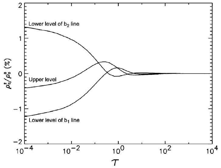
Figure 8.: The variation with the corresponding line optical depth of the fractional atomic polarization of the lower level of the Mg $b_{1}$ line, of the lower level of the Mg $b_{2}$ line and of the upper level of the Mg $b_{4}$ line. Each of the three optical depths $\tau$ is measured along the radial direction. The solar chromospheric model used is the VAL-C model of Vernazza et al. (1981).

What could be the physical origin and explanation of the above-mentioned observations? In a previous keynote article (cf. Trujillo Bueno 1999) I suggested that one could explain such spectropolarimetric observations if we had (at line-core optical depth unity along the line of sight) the following amounts of atomic polarization in the metastable lower levels of the Mg $b_{1}$ and $b_{2}$ lines:

• For the lower level of the $b_{2}$ line $\,\rightarrow\,\,$ $\sigma^{2}_{0}({l})\,{\approx}\,3X$.

• For the lower level of the $b_{1}$ line $\,\rightarrow\,\,$ $\sigma^{2}_{0}({l})\,{\approx}\,-2X$.

This “explanation” is based on the direct mapping that Eq. (30) implies: the observed polarization amplitudes are giving us directly the atomic polarization of the lower and upper levels at optical depth unity along the line of sight !

The crucial question now is: are these the atomic polarization values obtained from self-consistent multilevel scattering polarization calculations in semi-empirical models of the solar chromosphere? The answer is affirmative, as indeed results from a realistic multilevel coherency transfer calculation for a 19-level model atom for Mg I - Mg II (see Fig. 8). The results of this figure show that the metastable lower-levels of the Mg I $b_{1}$ and $b_{2}$ lines are polarized by the anisotropic radiation field of typical semi-empirical solar chromospheric models. The relative amplitudes of the calculated emergent polarizations of the three Mg $b$-lines at $\mu=0.1$ agree fairly well with the observations, with dichroism playing again a critical role.

7. The lower-level Hanle effect

The lower-level ${}^{2}{\rm D}_{3/2}$ of the Ca ii 8662 Å  line is metastable. Therefore, from Eq. (3), its atomic polarization and the emergent linear polarization have to be sensitive to milligauss fields. This is illustrated in Fig. 9, which shows the self-consistent values of the $\rho^{K}_{Q}$-elements for a horizontal field of 10 milligauss. The assumed horizontal field lies in the $xy$-plane of the reference system indicated in the “north solar pole” example of Figure 1. It is orientated at 45 degrees (measured from $x$ towards $y$). Fig. 9 shows the fractional population imbalances ($\rho^{2}_{0}/\rho^{0}_{0}$) and the coherences ($\rho^{2}_{Q}/\rho^{0}_{0}$, with $Q=1$ and $Q=2$) in percentage. Note that the 10 milligauss of the assumed horizontal field are sufficient to reduce the population imbalances of the ${}^{2}{\rm D}_{3/2}$ level by a factor 3 approximately (compare with the thin solid line of Fig. 7). Moreover, we now have non-zero coherences, which are of the same order of magnitude as the population imbalances themselves. The emergent fractional linear polarization ($Q/I$ and $U/I$) close to the stellar limb ($\mu=0.1$) and along the $x$-axis of Fig. 1 (i.e. a direction of observation with azimuth $\chi=0$ and $\mu=0.1$) is shown in Figure 10. Note that the $Q/I$ amplitude is a factor 3 smaller than the one corresponding to the zero magnetic field reference case of Fig. 7, and that $U/I$ is of the same order of magnitude as $Q/I$.

Figure 9.: The $\rho^{K}_{Q}$-elements for a horizontal field of 10 milligauss (solid lines) and of 10 gauss (dashed lines). Note that ${\rm Re}[\rho^{2}_{2}]/{\rho^{0}_{0}}=0$.

Figure 10.: The emergent $Q/I$ and $U/I$ of the 8662 Å  line corresponding to the two cases of Fig. 9. The simulated observation is along the $x$-axis of Fig. 1 (i.e. at $\chi=0$, but at $\mu=0.1$) and for an orientation of the assumed horizontal magnetic field as indicated in the text.

What is the physical origin of this $U/I$ profile? It is exclusively due to the coherences of the metastable lower-level of the Ca ii 8662 Å  line, because $\epsilon_{U}=0$, while $\eta_{U}{\neq}0$ (see the paragraph after Eq. 25). In fact, it is possible to derive Eddington–Barbier relations for the $Q/I$ and $U/I$ emergent polarizations due to the Hanle effect. This can be done along similar lines to those which lead to Eq. (30) for the unmagnetized reference case. Particularizing the Eddington–Barbier relation for $U/I$ to the direction of observation chosen to obtain the exact results of Fig. 10 (i.e. $\chi=0$) one obtains:

$$U/I\,{\approx}\,{\cal Z}\,\sqrt{3}\bigl{[}\sqrt{1-\mu^{2}}{\rm Im}(\sigma^{2}_{1})+\mu{\rm Im}(\sigma^{2}_{2})\bigr{]},$$ (37)

where $\sigma^{2}_{1}=\rho^{2}_{1}(l)/\rho^{0}_{0}(l)$ and $\sigma^{2}_{2}=\rho^{2}_{2}(l)/\rho^{0}_{0}(l)$ are the fractional coherences of the lower level of the 8662 Å  line at the spatial point along the line of sight where the optical depth at the selected frequency is unity. Note that ${\cal Z}{\approx}0.7$, with ${\cal Z}$ the symbol introduced after Eq. (30). Therefore, a positive detection of a $U/I$ signal close to the limb ($\mu=0.1$) would be a clean observational demonstration of the existence of metastable-level coherences.

Let us now consider what happens when the intensity of the same horizontal field is 10 gauss. As indicated by the dashed-lines of Figs. 9 and 10, the $\rho^{K}_{Q}$-elements and the emergent linear polarization are modified. The population imbalances of the ${}^{2}{\rm D}_{3/2}$ level are not destroyed and some of its coherences remain.. Note also that the emergent $Q/I$ in this saturated gauss regime still has a sizeable amplitude ($Q/I{\approx}0.4\%$), which is due to the atomic polarization of the metastable ${}^{2}{\rm D}_{3/2}$ lower-level. In other words, the atomic polarization of long-lived atomic levels in the solar chromosphere may still be sufficiently significant (even after the partial destruction caused by a 10 gauss purely horizontal field with a deterministic or random azimuth!) so as to be able to lead to emergent $Q/I$ signals in the observable range. In a forthcoming publication we will show in detail that a consistent explanation of the observed $Q/I$ in the three lines of the Ca ii IR triplet does not necessarily requires to constrain the magnetic field to be either extremely low (with $B{\leq}10$ milligauss) or vertically orientated (but with an intensity in the gauss regime). Note that I am not saying that the chromospheric magnetic field is predominantly horizontal. I am basically pointing out that some of the “enigmatic” features of the second solar spectrum are due to metastable-level atomic polarization and that the amount of this atomic polarization in topologically complex magnetic field scenarios with intensities in the gauss regime can still be sufficiently significant so as to lead to the observed $Q/I$ polarization amplitudes.

Finally, it may be found useful to distinguish between five Hanle effect regimes in relation with the polarization of a spectral line whose lower level is the ground or a metastable level. These Hanle regimes can be established according to the values of $\Gamma_{l}$ and $\Gamma_{u}$ and by noting that, for a given magnetic field intensity, $\Gamma_{l}\gg\Gamma_{u}$ (because the lower-level lifetime is about two orders of magnitude larger than the upper-level lifetime). As mentioned earlier, in this section we are using the reference system whose $z$-axis is directed along the radial direction of the star:

• Regime 1: $\Gamma_{l}\,\ll\,1\,\,\,$ and $\,\,\,\Gamma_{u}\,\ll\,1$

  In this regime the atomic alignment of the lower level of the line transition of interest is typically of the same order of magnitude as the upper-level alignment (i.e. $|\sigma^{2}_{0}(l)|\sim|\sigma^{2}_{0}(u)|$). We find here the maximum possible $Q/I$ amplitude.

• Regime 2: $\Gamma_{l}\,{\approx}\,1\,\,\,$ and $\,\,\,\Gamma_{u}\,\ll\,1$

  In this regime the emergent polarization is sensitive to milligauss fields.

• Regime 3: $\Gamma_{l}\,\gg\,1\,\,\,$ and $\,\,\,\Gamma_{u}\,\ll\,1$

  In this regime we have $|\sigma^{2}_{0}(l)|\ll|\sigma^{2}_{0}(u)|$.

• Regime 4: $\Gamma_{l}\,\gg\,1\,\,\,$ and $\,\,\,\Gamma_{u}\,{\sim}\,1$

  In this regime the emergent polarization is sensitive to magnetic fields in the gauss regime.

• Regime 5: $\Gamma_{l}\,\gg\,1\,\,\,$ and $\,\,\,\Gamma_{u}\,\gg 1\,$

  We again find that $|\sigma^{2}_{0}(l)|\sim|\sigma^{2}_{0}(u)|$, but with lower individual values for $|\sigma^{2}_{0}(l)|$ and $|\sigma^{2}_{0}(u)|$ than for the unmagnetized reference case. The emergent polarization is sensitive only to the field orientation. In this regime, one should find relative amplitudes of the linear polarizations observed in multiplets (e.g. in the Mg I $b$ lines) similar to those found for the unmagnetized reference case. This emphasizes the importance of an accurate quantification of the observed polarization amplitudes in order to infer correctly the intensity and inclination of the magnetic field.

8. Concluding remarks

This review article, besides providing an introduction to optical pumping, atomic polarization and the Hanle effect, has advanced some new results which we will publish in suitable journals during the following months. Of particular interest for the reader who looks at the Sun as a unique physics laboratory is the conclusion that the quiet solar chromosphere is a polarized vapor with optical properties similar to those of an anisotropic crystal.

On the other hand, the reader interested mainly in the remote sensing of solar and stellar magnetic fields should feel optimistic because the quest for understanding the physical origin of the “second solar spectrum” is now becoming one of the success stories of astrophysics. We had the theory (cf. Landi Degl’Innocenti 1983). We had the observations (cf. Stenflo and Keller 1997; Stenflo et al. 2000). And now we have the self-consistent radiative transfer modeling, which is the essential link between theory and observations. In the following years rigorous confrontations of observations of weak polarization signals with numerical simulations of scattering polarization and of the Hanle and Zeeman effects should lead to fundamental new insights in our understanding of solar photospheric and chromospheric magnetism.

Acknowledgments.

The author wishes to express his gratitude to Egidio Landi Degl’Innocenti and Rafael Manso Sainz for their collaboration and for valuable inputs and discussions, and to Michael Sigwarth for his invitation to participate in a highly interesting workshop. This work is part of the EC-TMR European Solar Magnetometry Network.

References

Blum, K. 1981, Density Matrix Theory and Applications, Plenum Press

Bohr, N. 1924, Naturwissenschaften, 12, 1115

Bommier, V. 1997 a, A&A, 328, 706

Bommier, V. 1997 b, A&A, 328, 726

Bommier, V., & Sahal-Bréchot, S. 1978, A&A, 69, 57

Brückner, G. 1963, Z. Astrophys., 58, 73

Cohen-Tannoudji, C. 1977, in Frontiers in Laser Spectroscopy, Ecole d’Eté des Houches 1975, North-Holland, Amsterdam

Cohen-Tannoudji, C., Dupont-Roc, J., & Grynberg, G. 1992, Atom-Photon Interactions: Basic Processes and Applications, John Wiley & Sons (p. 257)

Dittmann, O., Trujillo Bueno, J., Semel, M., & López Ariste, A. 2001, (this volume)

Fano, U. 1957, Rev. Mod. Phys., 29, 74

Faurobert-Scholl, M. 1996, in Solar Polarization, J.O. Stenflo & K.N. Nagendra (eds.), Kluwer Academic Publishers, p. 79

Gandorfer, A. 2000, The Second Solar Spectrum: a high spectral resolution polarimetric survey of scattering polarization at the solar limb in graphical representation, vdf Hochschulverlag AG an der ETH Zürich

Hanle, W. 1923, Naturwissenschaften, 11, 690

Hanle, W. 1924, Z. Phys., 30, 93

Hanle, W. 1925, Ergebnisse der Exakten Naturwissenschaften, 4, 214

Happer, W. 1972, Rev. Mod. Phys., 44, 169

Heisenberg, W. 1925, Z. Phys., 31, 617

House, L.L. 1970a, JQRST, 10, 909

House, L.L. 1970b, JQRST, 10, 1171

House, L.L. 1971, JQRST, 11, 367

Hyder, C.L. 1965, ApJ, 141, 1374

Ignace, R., Nordsieck, K.H. & Cassinelli, J.P. 1997, ApJ, 486, 550

Kastler, A. 1950, J. de Physique, 11, 255

Landi Degl’Innocenti, E. 1982, Sol. Phys., 79, 291

Landi Degl’Innocenti, E. 1983, Sol. Phys., 85, 3

Landi Degl’Innocenti, E. 1984, Sol. Phys., 91, 1

Landi Degl’Innocenti, E. 1985, Sol. Phys., 102, 1

Landi Degl’Innocenti, E. 1990, in Dynamics of Quiescent Prominences, V. Ruzdjak and E. Tandberg-Hanssen (eds.), Springer Verlag, Lecture Notes in Physics 363, 206

Landi Degl’Innocenti, E. 1992, in Solar Observations: Techniques and Interpretation, F. Sánchez, M. Collados and M. Vázquez (eds.), Cambridge University Press, p. 73

Landi Degl’Innocenti, E. 1998, Nature, 392, 256

Landi Degl’Innocenti, E., Landi Degl’Innocenti, M., & Landolfi, M. 1997, in Science with THEMIS, N. Mein and Sahal-Bréchot, S. (eds.), Paris Obs. Publ., p. 59

Landolfi, M. & Landi Degl’Innocenti, E. 1986, A&A, 167, 200

Leroy, J.L., 1989, in Dynamics and Structure of Quiescent Solar Prominences, E.R. Priest (ed.), Kluwer Academic Publishers, p. 77

Litvak, M.M. 1975, ApJ, 202, 58

Lyot, B. 1934, Compt. Rend. Acad. Sci., 198, 249

Manso Sainz, R., & Trujillo Bueno, J. 1999, in Solar Polarization, K. N. Nagendra and J. O. Stenflo (eds.), Kluwer, p. 143-156

Manso Sainz, R., & Trujillo Bueno, J. 2001a, (this volume)

Manso Sainz, R., & Trujillo Bueno, J. 2001b, ApJ, (in preparation)

Martínez Pillet, V., Trujillo Bueno, J., & Collados, M. 2001, (this volume)

Mihalas, D. 1978, Stellar Atmospheres, Freeman

Mitchell, A.C.G., & Zemansky, M.W. 1934, Resonance Radiation and Excited Atoms, Cambridge University Press

Moruzzi, G., & Strumia, F. 1991, (eds.), The Hanle Effect and Level-Crossing Spectroscopy, Plenum Press, New York

Omont, A. 1977, Prog. Quantum Electron., 5, 69

Redman, R.O. 1941, MNRAS, 101, 266

Sánchez Almeida, J., & Trujillo Bueno, J. 1999, ApJ, 526, 1013

Sánchez Almeida, J., & Lites, B. 2000, ApJ, 532, 1215

Stenflo, J.O. 1980, A&A, 84, 68

Stenflo, J.O. 1994, Solar Magnetic Fields: Polarized Radiation Diagnostics, Kluwer Academic Publishers

Stenflo, J.O. 1998, A&A, 338, 301

Stenflo, J.O., Twerenbold, D., Harvey, J.W., & Brault, J.W. 1983, A&A Suppl. Ser., 54, 505

Stenflo, J.O., & Keller, C. 1997, A&A, 321, 927

Stenflo, J.O., Keller, C., & Gandorfer, A. 2000, A&A, 355, 789

Trujillo Bueno, J. 1990, in New Windows to the Universe, Vol. 1, F. Sánchez & Vázquez (eds.), Cambridge University Press, p. 119

Trujillo Bueno, J. 1999, in Solar Polarization, K. N. Nagendra and J. O. Stenflo (eds.), Kluwer, p. 73-96

Trujillo Bueno, J. & Landi Degl’Innocenti, E. 1997, ApJ Letters, 482, 183

Trujillo Bueno, J. & Manso Sainz, R. 1999, ApJ, 516, 436

Trujillo Bueno, J., Collados, M., Paletou, F., & Molodij, G. 2001, (this volume)

Trujillo Bueno, J., Moreno Insertis, F., & Sánchez, F. (eds.) 2001, Astrophysical Spectropolarimetry, Cambridge University Press

Vernazza, J., Avrett, E., & Loeser, R. 1981, ApJ Suppl. Series, 45, 635

von Neumann, J. 1927, Göttingen Nachrichten, 245

Wiehr, E. 1978, A&A, 67, 257

Wood, R. W., & Ellett, A. 1923, Proc. R. Soc., 103, 396