Gamma-Rays from Intergalactic Shocks

Abstract

Structure formation in the intergalactic medium (IGM) produces large-scale, collisionless shock waves, where electrons can be accelerated to highly relativistic energies. Such electrons can Compton scatter cosmic microwave background photons up to $\gamma$-ray energies. We study the radiation emitted in this process using a hydrodynamic cosmological simulation of a $\Lambda\mbox{CDM}$ universe. The resulting radiation, extending beyond TeV energies, has roughly constant energy flux per decade in photon energy, in agreement with the predictions of Loeb & Waxman (2000). Assuming that a fraction $\xi_{e}=0.05$ of the shock thermal energy is transferred to the population of accelerated relativistic electrons, as inferred from collisionless non-relativistic shocks in the interstellar medium, we find that the energy flux of this radiation, $\epsilon^{2}(dJ/d\epsilon)\simeq 50-160\mbox{ eV cm}^{-2}\mbox{ s}^{-1}\mbox{ sr}^{-1}$, constitutes $\sim 10\%$ of the extragalactic $\gamma$-ray background flux. The associated $\gamma$-ray point-sources are too faint to account for the $\sim 60$ unidentified EGRET $\gamma$-ray sources, but GLAST should detect and resolve several $\gamma$-ray sources associated with large-scale IGM structures for $\xi_{e}\simeq 0.03$, and many more sources for larger $\xi_{e}$. The intergalactic origin of the shock-induced radiation can be verified through a cross-correlation with, e.g., the galaxy distribution that traces the same structure. Its shock-origin may be tested by cross-correlating its properties with radio synchrotron radiation, emitted as the same accelerated electrons gyrate in post-shock magnetic fields. We predict that GLAST and Čherenkov telescopes such as MAGIC, VERITAS and HESS should resolve $\gamma$-rays from nearby (redshifts $z\lesssim 0.01$) rich galaxy clusters, perhaps in the form of a $\sim 5-10\mbox{ Mpc}$ diameter ring-like emission tracing the cluster accretion shock, with luminous peaks at its intersections with galaxy filaments detectable even at $z\simeq 0.025$.

1 Introduction

In the past three decades, clear evidence has emerged indicating the existence of an extragalactic $\gamma$-ray background (EGRB). The origin of this radiation, however, has remained highly speculative. The first unambiguous detection of isotropic extragalactic $\gamma$-ray emission was obtained by the SAS-2 satellite at 1977. Subsequent experiments, especially the EGRET instrument aboard the Compton Gamma Ray Observatory (CGRO), have confirmed the existence of this radiation. These measurements indicate a generally isotropic (fluctuation amplitude $\lesssim 20\%$ on $\gtrsim 20^{\circ}$ scales) spectrum in the energy range 30 MeV-120 GeV, well fitted by a single power law, with photon number density per energy interval $dJ/d\epsilon\sim\epsilon^{-\left(2.10\pm 0.03\right)}$ Sreekumar et al. (1998). Known extragalactic sources, such as blazars, account for less than 7% of the EGRB, and unidentified blazars probably contribute no more than 25% of the radiation (Mukherjee & Chiang 2000; but for a different model see Stecker & Salamon 2001). Thus, most of the EGRB flux originates from a source yet to be identified.

Recently, Loeb & Waxman (2000) have proposed a model which attributes most of the EGRB flux to emission from large-scale structure-forming regions in the universe. Strong collisionless, non-relativistic shock waves characteristic of these regions accelerate particles to highly relativistic energies by the Fermi-acceleration mechanism, first discussed as sources of ultra-high energy cosmic rays by Norman, Melrose & Achterberg (1995) and by Kang, Ryu & Jones (1996). Electrons, accelerated in such shocks to highly relativistic energies with Lorentz factors up to $\gamma_{\mbox{\tiny max}}\sim 10^{7}$, scatter a small fraction of the cosmic microwave background (CMB) photons up to $\gamma$-ray energies, as inverse-Compton radiation. The estimated energy flux from this process per decade in photon energy, $\epsilon^{2}(dJ/d\epsilon)\approx 1.5\mbox{ keV}\mbox{ cm}^{-2}\mbox{ s}^{-1}\mbox{ sr}^{-1}$, is in good agreement with the detected EGRB, for typical cosmological parameters, provided that the shocked matter accumulated a present-day mass-average temperature $T\sim 10^{7}\mbox{ K}$, and that a fraction $\xi_{e}\approx 0.05$ of the associated thermal energy was transferred to the relativistic electrons. In this model, nearby rich galaxy clusters are expected to be bright $\gamma$-ray sources, as they host strong, dense shocks Loeb & Waxman (2000); Totani & Kitayama (2000).

Kawasaki & Totani (2001) report a correlation between a sample of high-latitude steady unidentified EGRET sources and pairs or groups of galaxy clusters, where strong accretion and merger shocks are expected. However, this sample is too small and the correlation too weak for it to be statistically significant. Enßlin et al. (2001) suggest that various features of the asymmetric radio plasma ejected from the giant radio galaxy NGC 315 can provide the first indication of a structure-formation shock in a filament of galaxies. According to the above model, such a shock should be accompanied by $\gamma$-ray emission, yet to be detected.

The model presented above has several interesting implications, other than an identification of the origin of the EGRB: $\gamma$-ray emission could be the first tracer of the undetected warm-hot intergalactic medium (WHIM), gas at temperatures $10^{5}\mbox{ K}\lesssim T\lesssim 10^{7}\mbox{ K}$ which is believed to contain a large fraction of the baryons in the low redshift universe (e.g. Davé et al. 2001a). The angular fluctuations in the EGRB should, according to the model, reflect the underlying forming structure, and thus serve as a diagnostic of intergalactic shocks. The relativistic electrons emit synchrotron radiation, as they gyrate in intergalactic magnetic fields. The resulting radio radiation, although weaker than the CMB, could have a fluctuating component dominating the CMB fluctuations at low ($\nu\lesssim 10\mbox{ GHz}$) frequencies Waxman & Loeb (2000). Inverse-Compton emission from shock-accelerated electrons in the hard X-ray (HXR) and extreme ultra-violet (EUV) bands was recently studied by Miniati et al. (2001). They find that such emission could account for a small fraction of the measured EUV excess, and for the entire HXR excess in a few reported galaxy clusters, provided that the latter contain relatively strong merger or accretion shocks.

In order to test this model, calibrate its free parameters and extract useful predictions, one must follow the evolution of structure in the intergalactic medium (IGM) in detail. The complex, non-linear processes and many scales involved, make this a difficult problem, rendering numerical simulations a powerful and indispensable tool. In this paper, we apply cosmological simulations to the problem of non-thermal emission from shock–accelerated electrons, and demonstrate how various EGRB predictions can be efficiently extracted from them. For this purpose, we have developed the necessary tools to localize intergalactic shocks in the simulations, inject the corresponding shock-accelerated electrons into the gas, and calculate the resulting radiation. We consider a hydrodynamic simulation of a $\Lambda\mbox{CDM}$ universe, currently considered the most successful theory of structure formation, which describes a flat universe containing dark matter and presently dominated by vacuum energy. The relativistic electrons are assumed to carry a fraction $\xi_{e}$ of the shock thermal energy. We adopt the value $\xi_{e}=0.05$, which we show is inferred from collisionless non-relativistic shocks in the interstellar medium.

Overall, we find an emitted inverse-Compton spectrum well-described by a mildly broken power law, $dJ/d\epsilon\sim\epsilon^{-2.04}$ in the energy range $10\mbox{ keV}-1\mbox{ GeV}$ and $dJ/d\epsilon\sim\epsilon^{-2.13}$ in the energy range $10\mbox{ GeV}-5\mbox{ TeV}$, in good agreement with the prediction of Loeb & Waxman (2000). The calculated energy flux (per decade in photon energy), $\epsilon^{2}(dJ/d\epsilon)=50-160\mbox{ eV}\mbox{ cm}^{-2}\mbox{ s}^{-1}\mbox{ sr}^{-1}$, constitutes $\sim 10\%$ of the EGRB flux and is smaller by a factor of $\sim 10$ than estimated above, mainly due to the lower present-day temperature reached by the simulation, $T_{0}\sim 4\times 10^{6}\mbox{ K}$, and its slower heating rate. We predict the existence of $\gamma$-ray halos, associated with large-scale structure. Although too faint to account for the EGRET unidentified $\gamma$-ray sources, several of these halos should be detectable by future experiments, such as the Gamma-Ray Large-Area Space Telescope (GLAST, planned to be launched in 2006), provided that $\xi_{e}\gtrsim 0.03$. The number of detectable sources is sensitive to the fraction of shock-energy transferred to the relativistic electrons, with $\sim 15$ well-resolved GLAST sources predicted for $\xi_{e}=0.05$. Detection of intergalactic shock-induced $\gamma$-ray sources may be used to calibrate the free parameter $\xi_{e}$. We examine images of such an object, as predicted to be produced by GLAST and by the Major Atmospheric Gamma-ray Imaging Čherenkov (MAGIC) telescope (expected to become operational during 2002). These images reveal an elliptic ring-like feature, of diameter corresponding to $5-10\mbox{ Mpc}$, surrounding a nearby ($z\simeq 0.012$) rich galaxy cluster. This ring, tracing the cluster accretion shock, has luminous peaks along its circumference, probably indicating the locations of intersections with galaxy filaments, channeling gas into the cluster.

We describe the Loeb-Waxman model in §2. We first consider the gross characteristics of intergalactic shocks based on order of magnitude estimates. In this context, we parameterize the distribution of accelerated electrons, and discuss the inverse-Compton and synchrotron radiation they emit. The simulation we chose to study and its basic predictions are described in §3. We discuss the underlying theory and cosmological model, present some characteristics of the simulated universe and examine its structure. Section 4 describes how EGRB predictions can be extracted from cosmological simulations in general and then focuses on the method applied to the simulation discussed in §3. In §5, we present our results regarding the radiation predicted from the simulation. We describe the resulting inverse-Compton spectrum, analyze the corresponding $\gamma$-ray sky maps and study the features and distribution of the simulated $\gamma$-ray sources. In §6 we discuss the implications of our results for future experiments and models. Appendix A contains some formulae used to calculate and integrate the radiation emitted by the accelerated electrons. Appendix B presents an algorithm devised to identify point sources in our simulated maps of the $\gamma$-ray sky.

2 Theory

This section describes the model for non-thermal emission from structure formation shocks proposed by Loeb and Waxman (2000), using simple order-of-magnitude estimates. First, we estimate the parameters of the large-scale shock waves involved in structure formation. Next, we discuss the high-energy electrons accelerated by such shocks. We evaluate the power index and cutoff of their distribution, and evaluate its normalization by estimating the efficiency of electron acceleration in intergalactic shocks. We conclude by calculating the radiation emitted by these electrons, mainly through inverse-Compton scattering off CMB photons. The estimates presented in this section needed for our numerical simulation are discussed in more detail in §4.

2.1 Intergalactic Shock Waves

Large-scale structure in the universe is believed to have evolved by the gravitational collapse of initially over-dense regions. As such an initial seed accreted increasing amounts of mass, large converging flows of matter were accelerated towards it, inevitably brought to a violent halt. This process resulted in large-scale shock waves, forming as massive gas flows collided with opposite flows or with the newly formed object. In the following, we concentrate our attention on the ’recent’ stages of structure formation, taking place at moderate to low redshifts ($z\lesssim 3$), and deduce some order of magnitude estimates of the resulting shock wave properties, following Cen & Ostriker (1999).

Linear theory of structure formation predicts that the length and mass scales of an object, forming (becoming non-linear) at these low redshifts, are roughly given by:

$$\lambda_{NL}(z)=\lambda_{0}\mbox{ }\frac{f(z)}{1+z}\quad\mbox{and}\quad M_{NL}(z)=M_{0}\mbox{ }f(z)^{3}\mbox{ ,}$$ (1)

where $\lambda_{0}$ and $M_{0}$ are the length and mass scales of structures forming at the present time and $f(z)$ is a slowly varying function of the redshift $z$, satisfying $f(z=0)=1$, such that smaller scales become non-linear first. These parameters are sensitive to the cosmological model. We use a ’concordance’ $\Lambda\mbox{CDM}$ model of Ostriker & Steinhardt (1995) - a flat universe with normalized vacuum energy density $\Omega_{\Lambda}=0.7$, matter energy density $\Omega_{M}=0.3$, baryon energy density $\Omega_{B}=0.04$, Hubble parameter $h=0.67$, and initial perturbation spectrum of slope $n=1$ and normalization $\sigma_{8}=0.9$ - to find:

$$\lambda_{0}\simeq 10h_{67}^{-1}\mbox{ Mpc}\quad\mbox{and}\quad M_{0}\simeq 1.5\times 10^{14}h_{67}^{-1}\left(\frac{\Omega_{M}}{0.3}\right)M_{\odot}\mbox{ ,}$$ (2)

where $h_{67}\equiv h/0.67$. The order of magnitude estimates obtained from linear theory in this subsection should be regarded with caution, as non-linear effects become important in the forming objects, and the phases of the perturbations can no longer be ignored. The distribution of the forming objects according to linear theory may be better estimated using the approach of Press & Schechter (1974).

Geometric considerations dictate that the gas in an object of size $\lambda$, collapsing over a time period $t_{\mbox{\tiny coll}}$, will achieve velocities of order $v\sim\lambda/t_{\mbox{\tiny coll}}$. Since a structure that became non-linear at redshift $z$ will collapse over a time period of order $t_{\mbox{\tiny coll}}\sim H(z)^{-1}$, where $H(z)$ is the Hubble parameter, the formation of such an object is expected to involve shocks with velocity:

$$v_{\mbox{\tiny sh}}(z)\simeq\mbox{ }k\mbox{ }\lambda_{NL}(z)\mbox{ }H(z)=v_{0}\mbox{ }\frac{f(z)h(z)}{1+z}\mbox{ ,}$$ (3)

where $k$ is a dimensionless number of order unity, $v_{0}\equiv k\lambda_{0}H_{0}$ is the typical shock velocity at $z=0$ and $h(z)\equiv H(z)/H(z=0)$. For the $\Lambda\mbox{CDM}$ model described above we find:

$$v_{0}\simeq 700\mbox{ km s}^{-1}\quad\mbox{and}\quad h(z)=\sqrt{\Omega_{\Lambda}+\Omega_{M}(1+z)^{3}}\mbox{ .}$$ (4)

Hence, the shock waves resulting from converging flows during structure formation in the IGM have a non-relativistic velocity similar to those of shocks surrounding supernova remnants (where accelerated particles are observed) and they are steadily growing in both scale and velocity.

The baryonic component may be treated as an ideal gas with an adiabatic index $\Gamma=5/3$, and is sufficiently rarefied such that the shocks concerned are collisionless. Using the Rankine-Hugoniot shock adiabat Landau & Lifshitz (1959), we can relate the shocked gas temperature to the shock velocity,

$$T(z)\simeq T_{0}\left[\frac{f(z)h(z)}{1+z}\right]^{2},$$ (5)

where $T_{0}\equiv[m_{p}/(\Gamma k_{B})](\alpha v_{0})^{2}$ is the temperature of gas, shocked at $z=0$, $k_{B}$ is the Boltzmann constant, and $\alpha\equiv c_{s,d}/v_{\mbox{\tiny sh}}$ is the ratio between the post-shock (downstream) sound velocity and the shock velocity (relative to the unshocked gas), approaching $\sim 0.56$ for a strong shock. For the $\Lambda\mbox{CDM}$ model above we find:

$$T_{0}\simeq 10^{7}\mbox{ K}\mbox{ .}$$ (6)

As we show in §3.2, this estimate of $T_{0}$ is indeed valid only to order of magnitude and appears to exceed the true value by a factor $\sim 3$.

2.2 Shock-Accelerated Electron Population

2.2.1 Acceleration Mechanism

Collisionless, non-relativistic shock waves are generally known to accelerate a power-law energy distribution of high-energy particles. This phenomenon has been observed in astrophysical shock waves on various scales, such as in shocks forming when the supersonic solar wind collides with planetary magnetospheres, in shocks surrounding supernovae (SNe) remnants in the interstellar medium, and probably also in shocks in many of the most active extragalactic sources: quasars and radio galaxies Drury (1983); Blandford & Eichler (1987). These power law distributions extend up to energies $\sim 100\mbox{ keV}$ in the Earth’s bow shock, to $\sim 100\mbox{ TeV}$ in SNe remnants Tanimori et al. (1998) where shock velocities are similar to those of intergalactic shocks, and over $10^{6}\mbox{ TeV}$ in Galactic cosmic rays.

Magnetic fields of amplitude $B\simeq 0.1-1\;\mu\mbox{G}$ are measured in halos of galaxy clusters Kronberg (1994) and in the Coma super-cluster Fusco-Femiano et al. (1999), suggesting that the IGM in which the shocks propagate is significantly magnetized. The measured magnetic field energy constitutes a fraction $\xi_{B}\simeq 0.01$ of the typical post-shock thermal energy in cluster environments Waxman & Loeb (2000).

Electrons are expected to be accelerated in intergalactic shocks by the Fermi acceleration mechanism. The velocity difference between the two sides of a shock front acts as a first-order acceleration mechanism ($dE/dt\sim E$), provided that slow-moving elastic scattering centers are embedded in the gas. Alfvén waves or magnetic inhomogeneities can function as such centers, scattering electrons through small angles and causing them to repeatedly diffuse through a shock front. Diffusion of the energetic electrons downstream, away from the shock front, provides a Poissonian escape route. These effects lead to a characteristic power-law distribution of the high-energy electrons steady-state number density:

$$\frac{dn_{e}}{dE_{e}}(E)\simeq AE^{-s}\mbox{ ,}$$ (7)

where $A$ is a normalization constant. The vast size and perpetual duration of these shocks enable them to dissipate significant fractions of their energies in this process.

The resulting distribution of high energy electrons can be calculated using the test-particle approximation Drury (1983); Blandford & Eichler (1987), where the test particles, accelerated by the shock, are assumed to have no effect on its structure. This approximation, valid for the acceleration of a small population of high energy electrons, predicts that the power-law index of the resulting population depends only on the kinematic structure of the shock front, and is given by:

$$s=\frac{r+2}{r-1}\mbox{ ,}$$ (8)

where $r$ is the compression factor of the shock. For a shock in an ideal gas, $r$ is given by:

$$\frac{1}{r}=\frac{\Gamma-1}{\Gamma+1}+\frac{2}{(\Gamma+1)M^{2}}\mbox{ ,}$$ (9)

where $M\equiv v_{\mbox{\tiny sh}}/c_{s,u}$ is the Mach number, and $v_{\mbox{\tiny sh}}$ and $c_{s,u}$ denote the shock velocity and the pre-shock (upstream) sound velocity, respectively. The shock waves of interest are generally strong, i.e. involve high ($M\gg 1$) Mach numbers. Hence, we find $r\approx(\Gamma+1)/(\Gamma-1)=4$, and thus $s\approx 2$.

In order to completely define the power-law distribution discussed, we must specify its normalization and the energy range over which it extends. The Fermi acceleration mechanism per-se does not impose stringent limits on the electron energies achieved, as long as the total energy carried by the accelerated electrons is small compared to the shock energy and the shock structure remains intact. The e-folding time for electron acceleration is given Loeb & Waxman (2000) by:

$$\tau_{\mbox{\tiny acc}}\sim\frac{r_{\mbox{\tiny L}}c}{v_{\mbox{\tiny sh}}^{2}}\approx 2\times 10^{4}\gamma_{7}(B_{-7}T_{d,7})^{-1}\mbox{ yr}\mbox{ ,}$$ (10)

where $r_{\mbox{\tiny L}}$ is the electron Larmor radius, $\gamma_{7}$ is the electron Lorentz factor - $\gamma_{e}$ - in units of $10^{7}$, $B_{-7}$ is the magnetic field in units of $0.1\;\mu\mbox{G}$, and $T_{d,7}$ is the downstream temperature of the gas, in $10^{7}\mbox{ K}$. This time-scale is much shorter than the shock lifetime. The limit on electron energy is therefore not determined by the acceleration process, but rather by cooling processes: electrons will stop accelerating once their cooling rate overcomes their acceleration rate. The dominant cooling process for the relevant parameters is inverse-Compton scattering of the electrons off CMB photons, with a characteristic cooling time:

$$\tau_{\mbox{\tiny IC}}=\frac{3m_{e}c}{4\sigma_{T}\gamma_{e}u_{\mbox{\tiny CMB}}}\simeq 2\times 10^{5}\gamma_{7}^{-1}(1+z)^{-4}\mbox{ yr}\mbox{ ,}$$ (11)

where $u_{\mbox{\tiny CMB}}$ is the CMB energy density. Synchrotron cooling of the electrons is less efficient, with a characteristic cooling time $\tau_{\mbox{\tiny syn}}=(u_{\mbox{\tiny CMB}}/u_{\mbox{\tiny B}})\tau_{\mbox{\tiny IC}}\simeq 10^{3}(B_{-7})^{-2}(1+z)^{4}\tau_{\mbox{\tiny IC}}$, where $u_{\mbox{\tiny B}}$ is the magnetic field energy density. Thus, inverse-Compton cooling is faster, as long as the downstream magnetic field satisfies $B<3(1+z)^{2}\;\mu\mbox{G}$. Equating $\tau_{\mbox{\tiny acc}}$ and $\tau_{\mbox{\tiny IC}}$ leads to the maximal Lorentz factor:

$$\gamma_{\mbox{\tiny max}}=3.3\times 10^{7}\left(B_{-7}T_{d,7}\right)^{1/2}(1+z)^{-2}\mbox{ .}$$ (12)

Since the electron energy loss is dominated by scattering of CMB photons, the flux of high energy photons produced by shock accelerated electrons depends only weakly on the magnetic field strength. The magnetic field determines, nevertheless, the highest energy of accelerated electrons, and hence the energy to which the inverse-Compton spectrum extends. For $B\simeq 0.1\mbox{ }\mu\mbox{G}$, as observed in cluster halos and which corresponds to a fraction $\xi_{B}\simeq 0.01$ of the post-shock thermal energy, the highest energy electrons up-scatter CMB photons to energy $\epsilon\simeq 1\mbox{ TeV}$. It should be pointed out here, that the observed sub-$\mu\mbox{G}$ fields may be representative of only the downstream (post shock) magnetic field strength, and that the upstream field may be significantly lower. In this case, the electron acceleration time will be longer, and the highest energy of accelerated electrons and of inverse-Compton photons may be significantly lower than estimated from equation (12). The strength of the upstream magnetic field depends on the processes leading to IGM magnetization, which are not yet known. Magnetic fields may be produced by turbulence induced by the large scale structure shocks themselves Kulsrud et al. (1997), by “contamination” by the first generation of stars Rees (1987) or radio sources Daly & Loeb (1990); Furlanetto & Loeb (2001), or by galactic winds (Kronberg, Lesch, & Hopp 1999). Under all these scenarios, the upstream magnetic field strength is not expected to be much smaller than the downstream field strength. Moreover, near equipartition fields are expected to be produced in collisionless shocks through the growth of electromagnetic instabilities, as indicated, for example, by observed supernovae remnants Helfand & Becker (1987); Cargill & Papadopoulos (1988) and $\gamma$-ray bursts Gruzinov & Waxman (1999); Medvedev & Loeb (1999), and there is evidence from supernovae remnant observations for an enhanced level of magnetic waves ahead of the shock front (Achterberg, Blandford, & Reynolds 1994) We therefore adopt for our estimates of the maximum electron energy magnetic field strengths corresponding to fixed $\xi_{B}\approx 0.01$, which reproduce the observed large scale field strengths.

We can now parameterize the normalization of the relativistic electron distribution, by assuming that a fraction $\xi_{e}$ of the thermal energy density induced by the shock, $\Delta u_{\mbox{\tiny th}}$, is transferred to these electrons:

$$u_{e}=\xi_{e}\Delta u_{\mbox{\tiny th}}=\frac{3}{2}\xi_{e}k_{B}\left(n_{d}T_{d}-n_{u}T_{u}\right)\mbox{ ,}$$ (13)

where $u_{e}\equiv m_{e}c^{2}\int_{1}^{\gamma_{\mbox{\tiny max}}}\gamma(dn_{e}/d\gamma)\,d\gamma$ is the total energy density of relativistic electrons and $u$ and $d$ subscripts indicate upstream (pre-shock) and downstream (post-shock) values, correspondingly. The gas number density, $n$, is related to the baryon number density, $n_{\mbox{\tiny bar}}$, by $n\langle m\rangle=n_{\mbox{\tiny bar}}m_{p}$, where $\langle m\rangle\approx 0.59m_{p}$ is the average particle mass in an ionized gas with a hydrogen mass fraction $\chi=0.76$. For strong shocks $s\simeq 2$ and $n_{u}T_{u}\ll n_{d}T_{d}$, thus $u_{e}\simeq A\ln{\gamma_{\mbox{\tiny max}}}$, and we find:

$$A\simeq\frac{3\xi_{e}n_{d}k_{B}T_{d}}{2\ln{\gamma_{\mbox{\tiny max}}}}\mbox{ .}$$ (14)

2.2.2 Acceleration Efficiency

The efficiency of particle acceleration in structure formation shocks, parameterized above by $\xi_{e}$, is an important parameter bearing linearly on our results, and thus deserves a special discussion. Although no existing model credibly calculates the acceleration efficiency, we can evaluate $\xi_{e}$ in intergalactic shocks by estimating the acceleration efficiency of other astrophysical shock waves.

The best analogy to intergalactic shocks may be found in supernova remnant (hereafter SNR) shocks, drawing on the similarity between the velocities of intergalactic shocks and SNR shocks, both of the order of $\sim 10^{3}\mbox{ km s}^{-1}$. The physics of shock waves is essentially determined by three parameters: the shock velocity $v_{\mbox{\tiny sh}}$, the pre-shock density $n_{u}$ and the pre-shock magnetic field $B_{u}$. Although the plasma density is very different in intergalactic shocks and in SNR shocks, the density may be extracted from the problem by measuring time in units of $\nu_{p,i}^{-1}$, where $\nu_{p,i}$ is the plasma frequency of the ions. The pre-shock magnetic field, parameterized by the cyclotron frequency of the ions, $\nu_{c,i}$, may not be scaled out of the problem as well. However, by comparing $\nu_{c,i}$ to the growth rate of electromagnetic instabilities in the shocked plasma, $\nu_{\mbox{\tiny e.m.}}\equiv\nu_{p,i}v_{\mbox{\tiny sh}}/c$, we find that for strong shocks $(\nu_{c,i}/\nu{\mbox{\tiny e.m.}})^{2}=\frac{B_{u}^{2}/8\pi}{(1/2)m_{p}n_{u}v_{\mbox{\tiny sh}}^{2}}\ll 1$. We thus assume there is a well behaved limit when this ratio approaches zero, suggesting that the pre-shock magnetic field has little effect on the characteristics of strong shocks. With this assumption, we expect to find much similarity between strong shocks in different environments, as long as their shock velocities are comparable.

The energy of the relativistic electrons accelerated in SNR shocks was calculated by several authors, using the multi-frequency emission from SNR’s, preferably remnants with TeV detection such as SN1006 (G$327.6-1.4$; Tanimori et al. 1998). Dyer et al. (2001) have modeled the multi-frequency emission from SN1006, finding a shock efficiency of $\xi_{e}=5.3\%$. The total energy they find in relativistic electrons constitutes a fraction $\eta_{e}\simeq 1.4\%$ out of the total supernova explosion energy ($W\simeq 5\times 10^{50}\mbox{ erg}$, as often quoted in the literature). Other authors Mastichiadis & de Jager (1996); Aharonian & Atoyan (1999) have estimated $\eta_{e}\simeq 1\%-2\%$ in SN1006, which corresponds to $\xi_{e}$ values in the range of $3.8\%-7.6\%$. Ellison, Slane and Gaensler (2001) have modeled the emission from supernova remnant $\mbox{G}347.3-0.5$, estimating the energy of relativistic electrons to constitute at least $1.2\%$ - and more likely $2.5\%$ - of the shock kinetic energy flux, corresponding to $2.5\%\lesssim\xi_{e}\simeq 5\%$.

An independent, less reliable method for estimating the electron acceleration efficiency relies on the observation, that relativistic ions accelerated in SNR shocks are dynamically significant Reynolds & Ellison (1992); Baring et al. (1999), and thus carry a large fraction (tens of percents, e.g. $\sim 50\%$ according to Ellison et al. 2001) of the post shock thermal energy. The efficiency of electron acceleration may then be found by estimating the ratio $\eta$ between the relativistic electron energy and the energy of relativistic ions. One may easily estimate the value of $\eta$ in interstellar medium cosmic rays: using the electron-to-proton ratio in a given energy, e.g. $1\%$ at GeV energies Barwick et al. (1998), correcting for electron cooling and integrating over energies, we find $\eta\simeq 3\%-4\%$, i.e. $\xi_{e}\simeq 1\%-2\%$. However, since there is no clear relation between $\eta$ in the interstellar medium and its value immediately behind the $\sim 10^{3}\mbox{ km s}^{-1}$ shocks found in SNR’s and in the intergalactic medium, this estimate of $\xi_{e}$ is controversial.

To summarize, a shock efficiency of $\xi_{e}\simeq 0.05$ is found from studies of supernovae remnants, characterized by shock velocities similar to those of intergalactic shocks and thus expected to exhibit similar behavior. Since there is some uncertainty in this parameter, values of $\xi_{e}$ in the range $0.02-0.10$ are considered plausible.

2.3 Resulting Radiation

In this subsection we calculate the radiation emitted by the relativistic electron population described above. As mentioned earlier, most of the energy is produced when the electrons inverse-Compton scatter CMB photons, resulting in a spectrum that extends up to TeV energies. A secondary radiation process is synchrotron emission from the electrons, gyrating in the magnetic field, resulting in a similarly sloped spectrum extending up to the infrared. Other radiative processes experienced by the electrons, such as Bremsstrahlung and Čherenkov radiation, are less important.

We begin by calculating the diffuse radiation, resulting from the various intergalactic shocks at recent epochs (moderate to low redshifts). We then focus our attention on a single forming structure and the angular distribution of relevant sources.

2.3.1 Diffuse Radiation

Inverse-Compton scattering describes the interaction of a free electron with radiation, when the electron kinetic energy exceeds the photon energy. In the ultra-relativistic limit, $\gamma_{e}\gg 1$, the average relative increase in photon energy is given by $\Delta\epsilon_{\gamma}/\epsilon_{\gamma}\simeq(4/3)\gamma_{e}^{2}$. Hence, an electron with energy $E_{e}=\gamma_{e}m_{e}c^{2}\gg m_{e}c^{2}$ will scatter a CMB photon to an average energy:

$$\langle\epsilon_{\gamma}\rangle\simeq\frac{4}{3}\gamma_{e}^{2}\epsilon_{\mbox{\tiny CMB}}=\zeta E_{e}^{2}\mbox{ ,}$$ (15)

where we have defined $\zeta\equiv(4/3)(m_{e}c^{2})^{-2}\epsilon_{\mbox{\tiny CMB}}$, and $\epsilon_{\mbox{\tiny CMB}}\simeq 3.83k_{B}T_{\mbox{\tiny CMB}}$ is the average energy of a CMB photon. The extent of the spectrum is determined by the electron range of energies: The maximal electron Lorentz factor, $\gamma_{\mbox{\tiny max}}\simeq 3.3\times 10^{7}$, is given by equation (12), and equation (11) imposes a minimal energy threshold, as electrons with Lorentz factors smaller than $\gamma_{\mbox{\tiny min}}\simeq 200$ hardly radiate during a Hubble time $\sim 10^{10}\mbox{ yr}$. Plugging this range of Lorentz factors into equation (15) shows that the emitted photon spectrum extends from $\sim 50\mbox{ eV}$ up to $\sim\mbox{TeV}$ energies.

The emitted spectrum may be found by assuming that each relativistic electron scatters a photon only once. This approximation, discussed in §4.3, gives qualitatively correct results and is exact for strong shocks. With this simplification, we find that the emitted energy density per unit photon energy is given by:

$$\frac{du_{\gamma}}{d\epsilon_{\gamma}}(\epsilon)=\frac{1}{2\zeta}\frac{dn_{e}}{dE_{e}}\left(\sqrt{\epsilon/\zeta}\right)=\frac{A}{2}\zeta^{s/2-1}\epsilon^{-s/2}\mbox{ .}$$ (16)

For a strong shock, where the electron number density satisfies $dn_{e}(E)/dE_{e}\simeq AE^{-2}$, this reduces to:

$$\epsilon\frac{du_{\gamma}}{d\epsilon_{\gamma}}(\epsilon)=A/2\mbox{ .}$$ (17)

For weak shocks, the approximation in equation (16) introduces a small numerical error ($\sim 2$), because the temporal evolution of the electron distribution affects the normalization of the resulting spectrum.

Determining the present-day photon spectrum requires integration over different shocks at various times. This, in turn, is determined by the redshift-dependence of the IGM parameters, and requires the use of non-linear structure formation theory. We note that the contribution of a shock that developed at redshift $z$ to the observed value of $\epsilon[du_{\gamma}(\epsilon)/d\epsilon_{\gamma}]$, is roughly proportional to $(1+z)^{-4}$. Thus, the main contribution to the spectrum observed today, especially at high photon energies, is expected to originate from recent shocks at $z\lesssim 0.5$. Assuming that a fraction $f_{\mbox{\tiny sh}}$ of the baryons in the universe were recently shocked to a temperature $T\simeq 10^{7}\mbox{ K}$, when $\gamma_{\mbox{\tiny max}}$ already approached $10^{7}$, we find from equation (14) and equation (17):

$$\epsilon\frac{du_{\gamma}^{\mbox{\tiny IC}}}{d\epsilon_{\gamma}}(\epsilon)\simeq 6.4\times 10^{-7}\mbox{ }T_{7}\left(\frac{\xi_{e}f_{\mbox{\tiny sh}}}{0.05}\right)\left(\frac{\Omega_{B}h_{67}^{2}}{0.04}\right)\mbox{ eV cm}^{-3}\mbox{ .}$$ (18)

The inverse-Compton flux per decade in photon energy thus becomes:

$$\epsilon^{2}\frac{dJ_{\gamma}^{\mbox{\tiny IC}}}{d\epsilon_{\gamma}}(\epsilon)\simeq 1.5\mbox{ }T_{7}\left(\frac{\xi_{e}f_{\mbox{\tiny sh}}}{0.05}\right)\left(\frac{\Omega_{B}h_{67}^{2}}{0.04}\right)\mbox{ keV cm}^{-2}\mbox{ s}^{-1}\mbox{ sr}^{-1}\mbox{ .}$$ (19)

This result is in excellent agreement with observational data, when supplemented by the contribution from unresolved point sources Loeb & Waxman (2000). One can employ the Press-Schechter mass function in order to carry out the time-integration over the radiation resulting from intergalactic shocks at various epochs. This approach gives, for slightly different cosmological parameters ($\Omega_{\Lambda}=0.65$, $\Omega_{B}=0.05$, $h=0.7$), a similar result Loeb & Waxman (2000):

$$\epsilon^{2}\frac{dJ_{\gamma}^{\mbox{\tiny IC,PS}}}{d\epsilon_{\gamma}}(\epsilon)\simeq 1.5\left(\frac{\xi_{e}}{0.05}\right)\mbox{ keV cm}^{-2}\mbox{ s}^{-1}\mbox{ sr}^{-1}\mbox{ .}$$ (20)

The synchrotron radiation emitted by the accelerated electrons may now be estimated. A relativistic electron with a Lorentz factor $\gamma_{e}$, gyrating in a magnetic field of amplitude $B$, emits photons with characteristic energy $\epsilon_{\gamma}\sim[(\hbar eB)/(m_{e}c)]\gamma_{e}^{2}$. Synchrotron radiation is thus expected in photon energies ranging from $10^{-12}\mbox{ eV}$ and up to $1\mbox{ eV}$. The emitted flux can be crudely estimated as:

$$\epsilon^{2}\frac{dJ_{\gamma}^{\mbox{\tiny syn}}}{d\epsilon_{\gamma}}(\epsilon) \simeq \epsilon^{2}\frac{dJ_{\gamma}^{\mbox{\tiny IC}}}{d\epsilon_{\gamma}}(\epsilon)\cdot\frac{u_{B}}{u_{\mbox{\tiny CMB}}}$$ (21)

$$\simeq 1.5\mbox{ }T_{7}B_{-7}^{2}\left(\frac{\xi_{e}f_{\mbox{\tiny sh}}}{0.05}\right)\left(\frac{\Omega_{B}h_{67}^{2}}{0.04}\right)\mbox{ eV cm}^{-2}\mbox{ s}^{-1}\mbox{ sr}^{-1}\mbox{ ,}$$

whereas a more careful approach is to assume that the energy density of the post-shock magnetic field constitutes a fraction $\xi_{B}$ of the shock-induced thermal energy. This assumption, combined with the Press-Schechter mass function, leads to a similar (somewhat higher) flux:

$$\epsilon^{2}\frac{dJ_{\gamma}^{\mbox{\tiny syn,PS}}}{d\epsilon_{\gamma}}(\epsilon)\simeq 3\left(\frac{\xi_{e}}{0.05}\right)\left(\frac{\xi_{B}}{0.01}\right)\mbox{ eV cm}^{-2}\mbox{ s}^{-1}\mbox{ sr}^{-1}\mbox{ ,}$$ (22)

where a typical value $\xi_{B}=0.01$ produces magnetic fields consistent with observations of the outer halos of X-ray clusters Waxman & Loeb (2000).

2.3.2 Radiation From Forming Objects, Angular Statistics

We start with the general case of an astrophysical object formed recently, and calculate its inverse-Compton luminosity. We assume that the object accretes mass at a rate $\dot{M}$, heating it up to a temperature $T$ by strong shocks. The baryon number accretion rate is thus given by $\dot{M}(\Omega_{B}/\Omega_{M})\langle m\rangle^{-1}$. We assume, as previously, that a fraction $\xi_{e}$ of the post-shock thermal energy is converted into relativistic electrons. The maximal electron Lorentz factor $\gamma_{\mbox{\tiny max}}$ is determined from equation (12), and depends on the assumed magnetic field. Electrons with cooling time longer than the virialization time of the object, $t_{\mbox{\tiny vir}}$, will not have sufficient time to radiate a significant fraction of their energy. This introduces a low-energy cutoff in the emitted spectrum, at photon energy $\epsilon_{\mbox{\tiny min}}=(4/3)\gamma_{\mbox{\tiny min}}^{2}\epsilon_{\mbox{\tiny CMB}}$, where $\gamma_{\mbox{\tiny min}}\simeq 2\times 10^{12}\mbox{ yr}/t_{\mbox{\tiny vir}}$. This effect reduces the total luminosity by a factor $\ln{\left(\gamma_{\mbox{\tiny max}}/\gamma_{\mbox{\tiny min}}\right)}/\ln{\gamma_{\mbox{\tiny max}}}$. Combining these considerations, we find that the total and specific luminosities of the object are given by:

$$L^{\mbox{\tiny IC}}=\dot{M}\frac{\Omega_{B}}{\Omega_{M}}\langle m\rangle^{-1}\mbox{ }\xi_{e}\frac{3}{2}k_{B}T\mbox{ }\frac{\ln{\left(\gamma_{\mbox{\tiny max}}/\gamma_{\mbox{\tiny min}}\right)}}{\ln{\gamma_{\mbox{\tiny max}}}}\mbox{ ,}$$ (23)

and:

$$\epsilon_{\gamma}\frac{dL^{\mbox{\tiny IC}}}{d\epsilon_{\gamma}}=\frac{L^{\mbox{\tiny IC}}}{2\ln{\left(\gamma_{\mbox{\tiny max}}/\gamma_{\mbox{\tiny min}}\right)}}\quad\mbox{for energies}\quad 1\left(\frac{\gamma_{\mbox{\tiny min}}}{10^{3}}\right)^{2}\mbox{ keV}\lesssim\epsilon_{\gamma}\lesssim 0.1\left(\frac{\gamma_{\mbox{\tiny max}}}{10^{7}}\right)^{2}\mbox{ TeV}\mbox{ .}$$ (24)

Structure formation at the current epoch produces dense, large-scale sheets and filaments, entangled in space. The densest regions appear at the intersections of these features, around the locations of galaxy clusters. As an example, we consider such a galaxy cluster. The typical gas mass involved in the formation of a cluster is $M_{\mbox{\tiny gas}}\simeq 10^{14}M_{\odot}$, accreting over a virialization time $t_{\mbox{\tiny vir}}\sim 10^{9}\mbox{ yr}$ and shocked to a temperature $T_{\mbox{\tiny gas}}\gtrsim 10^{7}\mbox{ K}$. A magnetic field of amplitude $B\simeq 0.1\;\mu\mbox{G}$, as suggested by observations, gives $\gamma_{\mbox{\tiny min}}\simeq 2000$ and $\gamma_{\mbox{\tiny max}}\simeq 3.3\times 10^{7}$. Whence,

$$L_{\mbox{\tiny cluster}}^{\mbox{\tiny IC}}\simeq 2.2\times 10^{45}\left(\frac{\xi_{e}}{0.05}\right)\left(\frac{k_{B}T_{\mbox{\tiny gas}}}{5\mbox{ keV}}\right)\left(\frac{M_{\mbox{\tiny gas}}}{10^{14}M_{\odot}}\right)\left(\frac{t_{\mbox{\tiny vir}}}{10^{9}\mbox{ yr}}\right)^{-1}\mbox{ erg s}^{-1}\mbox{ ,}$$ (25)

and:

$$\epsilon_{\gamma}\frac{dL_{\mbox{\tiny cluster}}^{\mbox{\tiny IC}}}{d\epsilon_{\gamma}}\simeq 0.05L_{\mbox{\tiny cluster}}^{\mbox{\tiny IC}}\quad\mbox{for energies}\quad 5\mbox{ keV}\lesssim\epsilon_{\gamma}\lesssim 1\mbox{ TeV}\mbox{ .}$$ (26)

A comprehensive discussion of particle acceleration in galaxy clusters and the resulting inverse-Compton radiation up to hard X-rays, may be found in Sarazin (1999).

The angular statistics of the radiation predicted by the model can be investigated by simplifying assumptions regarding the mass distribution. Waxman and Loeb (2000) calculated the angular correlation of the spectrum using the Press-Schechter mass function. On sub-degree angles they find fluctuations $\gtrsim 40\%$ in the inverse-Compton spectrum and fluctuations $>100\%$ in the synchrotron spectrum.

3 Simulation

The previous section presented some order of magnitude estimates, leading from linear or non-linear structure formation theories to an EGRB spectrum, that roughly matches present-day observations. However, further progress along this route is severely compromised by the complexity and non-linearity of structure formation. This situation naturally calls for the use of cosmological simulations that incorporate hydrodynamical effects. For this project, we analyze a simulation of a $\Lambda\mbox{CDM}$ cosmology. In the following, we describe the cosmological model and background theory of this simulation, and discuss some characteristics of the simulated universe and the predicted underlying structure.

3.1 Model and Theory

The cosmological model adopted in the simulation is the ’concordance’ $\Lambda\mbox{CDM}$ model of Ostriker & Steinhardt (1995), presented in §2.1. An initial Harrison-Zel’dovich spectrum of fluctuations was assumed, and linear structure formation theory Eisenstein & Hu (1998) employed to predict the resulting spectrum at a certain redshift $z_{\mbox{\tiny start}}$, providing initial conditions for the simulation. The various parameters of the cosmological model are summarized in Table 1 (see e.g. Springel, White & Hernquist 2001b).

The simulation was performed using the TreeSPH code GADGET (Springel, Yoshida, & White 2001a). This code, designed for both serial and parallel computers, is intended for collisionless and gas-dynamical cosmological simulations.

Dark matter is modeled by the code as a self-gravitating collisionless fluid, represented by a large number $N_{\mbox{\tiny DM}}$ of particles. Newton’s gravitational potential is modified by introducing a spline softening at small separations, equivalent to treating each particle as a normalized spline mass distribution, instead of as a point mass (see, e.g. Hernquist & Katz 1989). This modification is necessary in order to suppress large angle scattering in two-body collisions. Poisson’s equation is solved using a hierarchical tree algorithm Barnes & Hut (1986).

The baryonic component of the universe is modeled by the simulation as an ideal gas, with an adiabatic index $\Gamma=5/3$, and is represented by a large number of particles, similar to the dark matter. The gas is governed by the continuity equation:

$$\frac{d\rho}{dt}+\rho\mathbf{\nabla}\cdot\mathbf{v}=0\mbox{ ,}$$ (27)

the Euler (momentum) equation:

$$\rho\frac{d\mathbf{v}}{dt}=-\mathbf{\nabla}P-\rho\mathbf{\nabla}\Phi+\mathbf{\nabla}\cdot\overline{\Sigma}\mbox{ ,}$$ (28)

and the thermal energy equation (the first law of thermodynamics):

$$\frac{du}{dt}=-\frac{P}{\rho}\mathbf{\nabla}\cdot\mathbf{v}-\frac{1}{\rho}\overline{\Sigma}_{ij}\partial_{i}\mathbf{v}_{j}-\frac{\Lambda(u,\rho)}{\rho}\mbox{ ,}$$ (29)

where $P$, $\rho$, $u$ and $\mathbf{v}$ are the pressure, mass density, thermal energy per unit mass and velocity of a gas element; $\Phi$ is the gravitational potential, found from Poisson’s equation:

$$\nabla^{2}\Phi(r,t)=4\pi G\rho(r,t)\mbox{ ;}$$ (30)

and we have used Lagrangian derivatives:

$$\frac{d}{dt}=\frac{\partial}{\partial t}+\mathbf{v}\mathbf{\cdot}\mathbf{\nabla}\mbox{ .}$$ (31)

An artificial viscosity Steinmetz (1996) term $\overline{\Sigma}$ was added to the above equations, in order to capture shocks. A cooling function $\Lambda(u,\rho)$ may be included in the energy equation, to incorporate radiative cooling processes.

These hydrodynamical equations are solved using the SPH - Smoothed Particle Hydrodynamics - technique (Lucy 1977; Gingold & Monaghan 1977; Monaghan 1992), well suited for non-axisymmetric three-dimensional astrophysical problems. The version of the code used for the simulation employs adaptive SPH smoothing lengths, such that each particle has a constant number $N_{s}$ of neighbors lying within its kernel. The hydrodynamical equations and their solutions in the formalism of this version of SPH appear in Springel et al. (2001a). We note that the simulation analyzed in this paper employed a formulation of SPH which does not rigorously conserve entropy in adiabatic parts of the flow (for a discussion, see Hernquist 1993, Springel & Hernquist 2002a).

The code simulates the evolution of dark matter and gas (hereafter: SPH) particles within a finite simulation box of comoving size $L_{\mbox{\tiny com}}^{3}$, using periodic boundary conditions. Due to technical reasons, to be discussed in the next section, we have chosen to employ a simulation that did not include radiative cooling processes. Radiative cooling, dominated by Bremsstrahlung and line emission at the epoch of interest, is sub-dominant relative to inverse-Compton emission from relativistic electrons in all but the densest regions within the cores of clusters where the baryon number density exceeds $\sim 10^{-3}\mbox{ cm}^{-3}$, and in cold ($T\lesssim 10^{4}\mbox{ K}$), dilute regions. We discuss the significance of radiative cooling towards the end of this section. The simulation neglected feedback from star formation and supernovae. The code parameters used in the simulation are presented in Table 2.

3.2 Resulting Structure

The simulation chosen for the project, as most cosmological simulations, predicts a highly structured IGM in the present-day universe, as illustrated in Figure 1. Several hot and dense objects are spread throughout space, separated by large empty voids. The largest of these structures are sheet-like objects (pancakes) and filaments, entangled in space, some as long as $\sim 100\mbox{ Mpc}$. At the intersection of the filaments appear denser, spheroidal objects, with typical size $\sim 1\mbox{ Mpc}$, where galaxy clusters are formed. Simulations predict that the pancake-resembling objects are the first large structures to appear. At the intersections of these pancakes, filaments emerge, which in turn intersect and drain mass into spheroidal objects. At the large scales discussed, dark matter and baryons essentially trace the same structure.

The objects described above are significantly denser than their surroundings. Thus, the last stages of their evolution are dominated by non-linear processes. These processes are mainly gravitational, though other physical processes, such as non-linear gas dynamics and radiative cooling (when included), influence these stages of structure evolution as well.

It is instructive to examine the thermodynamic evolution of the universe, by applying some averaging schemes to the temperature and density at different epochs, as shown in Figure 2. The mass averaged temperature is notably higher than the volume averaged temperature, because hot regions are typically much denser, leaving most of the volume with a dilute, cooler gas (e.g. Davé et al. 1999). The present-day averaged temperature reached by the simulation, $T(z=0)=3.9\times 10^{6}\mbox{ K}$ (see Figure 2), is significantly lower than the order-of-magnitude estimate presented earlier. (Note that the approximation of eq. [5] is in rough agreement with the mass averaged temperature, although deviating towards higher temperatures at recent times.) Furthermore, the simulation result for the present-day mass averaged temperature is lower than that predicted by Cen & Ostriker (1999) by a factor $\sim 2.5$, but in good agreement with the results of e.g. Refregier et al. (2000), Croft et al. (2001), and Refregier & Teyssier (2000). R. Cen (private communication) informs us that revised estimates for the temperature evolution of the Cen & Ostriker (1999) simulation, correcting for an error in the integration of the thermal energy equation, now actually lie below the other simulation results.

The volume averaged density is proportional to $(1+z)^{3}$, due to the expansion of the universe, whereas the approximately constant mass averaged density indicates that much of the mass has virialized. The temperature averaged density is higher than the volume averaged density, due to the above mentioned correlation between hot and dense regions. This (temperature averaged) density decreases in time, growing closer to the volume averaged density, as the dilute gas surrounding virialized structures heats up.

We examine the effect of radiative cooling by super-imposing cooling-time contours on the distribution of mass in the temperature-density phase-space (Figure 3, left). The figure suggests that radiative cooling has important effects on the present-day gas, residing in the most dense, hot regions and in the most cold, dilute regions. The cooling time in these volumes due to Bremsstrahlung and line emission, $t_{\mbox{\tiny cool}}$, is comparable to or smaller than the dynamical time, $t_{\mbox{\tiny H}}\sim H^{-1}$. Such regions, where $t_{\mbox{\tiny cool}}<t_{\mbox{\tiny H}}$, presently contain approximately $25\%$ of the gas mass, and a progressively larger mass fraction at higher redshifts (Figure 3, right). The dense and hot regions, where radiative cooling is significant, are associated with the cores of clusters, well beyond the accretion shock fronts of interest and should thus have little effect on our results, although the weaker merger and flow shocks may be affected. Radiative effects in the cold, dilute regions cools the collapsing gas and may result in slightly stronger accretion shocks. However, as these regions are cold to begin with, this effect should be unimportant.

4 Method

Next we discuss how cosmological simulations can be exploited to yield various predictions regarding the EGRB, according to the Loeb-Waxman model. Parts of the discussion are specific to the cosmological simulation chosen for the project, introduced in the previous section, and to the EGRB extraction schemes used. Predictions of shock-induced radiation are obtained from the simulation in three basic steps: First, the simulation is used to keep track of the forming structures and locate the shocks involved in their virialization. Second, relativistic electron populations are injected into the shocked gas, according to the predictions of the Fermi acceleration mechanism. And third, the radiation emitted by the relativistic electrons is calculated and integrated to give measurable EGRB features. The organization of this section corresponds to these three steps.

4.1 Extracting Shocks

Since shock waves are discontinuities in the thermodynamic quantities, locating shocks involves identifying large gradients in the properties of the gas. Gradients of quantities such as pressure, temperature or velocity, can be calculated directly from a simulation. In our case, this requires SPH kernel interpolation, as described in the previous section. Next, one can search for gradients larger than some imposed thresholds. These would imply the presence of shocks, stronger than a corresponding shock strength. The shock front could then be traced out, yielding the shock topology and the jump conditions across the shock, which can in turn be checked to see if they satisfy the Rankine-Hugoniot adiabat.

Such an approach was adopted by Miniati et al. (2000), using simulations based on a version of the total variation diminishing scheme (TVD), designed to capture strong shocks Ryu et al. (1993). They identified very strong accretion shocks with Mach numbers $M$ of up to $10^{3}$ around the filaments and halos of their simulations. These halos exhibit, in addition, weaker shocks ($M\sim 3-10$), originating from the merger of structures or from accretion shocks into old structures, already embedded within newly formed halos. Combined, these shocks lead to a complicated pattern of inter-winding shocks. Miniati et al. find that the jump conditions, imposed by a shock, are altered by adiabatic gravitational compression, especially when the shock is close to the core of a cluster. Since the limited simulation resolution renders these two effects inseparable, shock parameters were extracted under the assumption that gravitational effects are isothermal.

4.1.1 Shock-Extraction Scheme

Since we are interested more in the shocked gas than in the topology of shocks, we find SPH simulations sufficient for our needs, although they do provide limited shock front resolution. This enables us to adopt a simpler approach for locating shocks, appropriate for Lagrangian simulations such as SPH. This method involves following a gas element throughout the simulation, searching for rapid increases in its entropy. In cosmological simulations, entropy changes of the gas should result only from shock waves or from cooling processes. This is the reason we have chosen, for simplicity, to work with a simulation in which radiative cooling is neglected, shown in the previous section to yield reliable shocks. In such a simulation, the entropy of the gas should only increase, and do so in discrete steps, decisively indicating the presence of shocks. Ideally, one could then identify all entropy ’jumps’ as shock waves, determining their space-time coordinates. The thermodynamic jump conditions across a shock could then be found, by comparing the thermodynamic parameters of the gas element before ($T_{i}$, $\rho_{i}$) and after ($T_{f}$, $\rho_{f}$) passing through the shock, directly, or using the entropy-change, $\Delta S=C_{V}\ln{\left[(T_{f}/T_{i})(\rho_{f}/\rho_{i})^{(1-\Gamma)}\right]}$, induced by the shock. Using the Rankine-Hugoniot adiabat, we find that the compression factor $r$ of a shock - related to its Mach number by equation (9) - can be determined from $\Delta S$ according to:

$$\Delta S_{*}\equiv C_{V}^{-1}\Delta S=\ln{\left[\frac{r(\Gamma+1)-(\Gamma-1)}{(\Gamma+1)-r(\Gamma-1)}r^{-\Gamma}\right]}\mbox{ .}$$ (32)

In SPH simulations, one can choose the SPH particles themselves as the gas elements to be followed, since they are of constant mass and the simulation is Lagrangian. This technically simplifies our shock-locating scheme, as kernel interpolation becomes unnecessary. It is instructive to study the distribution of mass - i.e. SPH particles - that accumulated various entropy-changes during recent epochs. Figure 4 (left) gives this distribution in terms of the mass fraction $f(\Delta S_{*}^{\prime})=m_{\mbox{\tiny tot}}^{-1}dm(\Delta S_{*}^{\prime})/d\Delta S_{*}$ of SPH particles that accumulated a normalized entropy change $\Delta S_{*}^{\prime}$ between $z=2$ and $z=0$, where $m_{\mbox{\tiny tot}}$ is the total mass of SPH particles. First, note that a small fraction of the gas experienced negative entropy changes, most probably as a result of lack of strict entropy conservation in the absence of shocks, owing to the particular formulation of SPH used for this simulation (see, e.g. Springel & Hernquist 2002a). The entropy-difference distribution among such particles resembles a normal distribution, consistent with accumulating noise. The shape of the remaining distribution has an interesting structure, suggesting a pronounced population of ’weak’ shocks, with $M\sim 3-10$, and a large population of stronger shocks, with Mach numbers up to a few $10^{3}$, in agreement with Miniati et al. (2000).

In order to determine the location and temporal duration of shock waves, one must examine the simulated gas in sufficiently short time intervals. This is also necessary in order to identify multiple shocks suffered by an SPH particle, as the effect of consecutive shocks is not additive, although the entropy change they induce is. We chose to examine snapshots of the simulated gas, separated by the simulation-box light-crossing time, as illustrated in Appendix A. For the mass resolution of the simulation, the entropy-increase experienced by most shocked particles is spread over several of these snapshots, indicating that shorter time intervals are not required. With the time intervals that were chosen, the entropy-difference distribution between any two snapshots (Figure 4, right) is fairly constant throughout the period of interest. Based on this distribution, we impose a minimal threshold $\Delta S_{*}^{\mbox{\tiny min}}$, such that only particles experiencing a larger entropy-increase between two consecutive snapshots are considered shocked. A threshold value $\Delta S_{*}^{\mbox{\tiny min}}=0.4$ was found to be reasonable, considering numerical noise, although it entails the danger of eliminating some of the mildly weak shocks ($M\lesssim 10$), if an SPH particle requires many snapshots to cross such a shock. The fact that only $\sim 10\%$ of the gas suffers entropy-changes larger than $\Delta S_{*}^{\mbox{\tiny min}}$ simplifies the computational work considerably. Demanding that the entropy increases at least by $n_{s}\Delta S_{*}^{\mbox{\tiny min}}$ during $n_{s}=2$ consecutive snapshots, and dismissing shocked particles that did not reach a temperature $T_{\mbox{\tiny min}}\equiv 10^{5}\mbox{ K}$ by the present time, further simplifies the analysis. Our final results do not strongly depend upon the choice of these threshold values near those specified above. Note that with finite resolution, SPH particles may pass through a shock in a period longer than the snapshot temporal resolution. The simulation must thus be traced down to $z<0$ values in order to capture all recent shocks.

The temperature jump across a shock determines the thermal energy (per particle) it adds to the gas, $\Delta U_{\mbox{\tiny th}}/N=(\Gamma-1)^{-1}k_{B}(T_{d}-T_{u})$, and is thus vital for the calculation of shock-induced radiation. In principle, this jump could be found directly, by comparing the temperature of the shocked SPH particle before and after a shock takes place. However, with finite simulation resolution, this approach leads to errors, due to significant adiabatic heating or cooling of the particle in parallel to the shock. In some extreme cases, we even found the shocked particle cooler than it was prior to the shock. (A similar problem when radiative cooling is active has been identified by e.g. Hutchings & Thomas [2000] and Martel & Shapiro [2001].) A partial remedy for this problem is to assume that the entropy induced by the shock - and thus the compression factor - was correctly determined so that the state of the shocked particle can be deduced from its state prior to the shock, or vice versa. Indeed, neither the pre-shock state of the particle nor its post-shock state are accurately known, due to the inaccurate shock timing and ongoing adiabatic processes, leading to some inevitable error. We chose to regard the temperature of the gas, before the shock was detected, as the true pre-shock temperature: $T_{u}\equiv T_{i}$. Hence, we take:

$$T_{d}=T_{i}r^{(\Gamma-1)}e^{\Delta S_{*}}\mbox{ }$$ (33)

as the post-shock temperature, where $r$ and $\Delta S_{*}$ are related by equation (32). This choice yields more realistic results than the alternative, $T_{d}=T_{f}$, as discussed in §4.1.2.

4.1.2 Shock-Extraction Results

The shock-extraction scheme, described above, identifies shocks in $\sim 40\%$ of the simulated gas mass during recent epochs ($z<2$), where about $30\%$ of the baryons were shocked at least once (Figure 5, left). Most identified shocks are concentrated around the halos in the simulation, although filaments and sheets are traced out as well. In some cases, but not always, shock fronts can be identified (Figure 6).

The distribution of entropy-differences, accumulated by identified shocks (Figure 5, right), suggests that most of the strong shocks with Mach numbers in the range $M>10^{2}$ were located. It confirms, however, our suspicion of loosing most of the ’weak’ shock population ($M\sim 3-10$). In such shocks, the entropy-change suffered by a single particle is spread over many snapshots, and is thus eliminated by the imposed entropy-change threshold. Figure 5 (right) suggests that some of the very large accumulating entropy-increases, suffered by an SPH particle, result from multiple shocks. Separating the shocks in such cases results in a population of weaker shocks, artificially concentrated at the threshold shock strength ($M\sim 4$).

As a ’sanity check’ of the proposed shock-location and energy-evaluation schemes, we compare the thermal energy gain of the simulation to the evaluated energy, induced by the identified shocks. We find that the energy, injected by our shocks, constitutes a fraction $f_{\mbox{\tiny sh}}\sim 2/3$ of the total thermal energy gained by the simulated gas (see Table 3 and Figure 5, left). For comparison, in the estimates of §2.1 we took $f_{\mbox{\tiny sh}}=1$. Miniati et al. (2000) find, for a slightly different $\Lambda\mbox{CDM}$ model ($\Lambda=0.55$, $h=0.6$), that the energy passing through shocks with Mach numbers $M>10^{2}$ between redshift $z=1.5$ and today, approximately equals the present-day thermal energy of their simulation.

The above results were obtained by estimating the energy of an SPH particle, gained when passing through a shock, based on its temperature before passing through the shock (i.e. taking $T_{u}=T_{i}$). Estimating this energy gain based on the temperature after passing through the shock (i.e. taking $T_{d}=T_{f}$) results in shock energies lower, on average, by a factor $\sim 4.5$. This result is a combined effect of the low resolution of the simulation and adiabatic cooling, taking place in parallel to the shock.

We find the shock-extraction results described above reassuring, as they indicate that the proposed shock location-and-evaluation recipe captures most of the strong shocks, and measures their energy reasonably well. Better performance of this algorithm may be achieved by using simulations with a higher mass resolution and with a more accurate handling of adiabatic flows (e.g. Springel & Hernquist 2002a). It should be stressed that the elimination of weak shocks by imposing an entropy threshold for shock identification has only a small effect on the predicted diffuse $\gamma$-ray radiation, especially at high energies. First, the consistency check described above verifies that the energy injected by weak shocks is small compared to the energy injected by strong shocks: accounting for all weak shocks may increase the integrated flux at most by a factor of $\sim 1.5$. Second, the contribution of weak shocks to the $\gamma$-ray emission, especially at high photon energies, is small due to the steep distribution of the electrons accelerated by such shocks, reducing their $\gamma$-ray efficiency. At $10\mbox{ GeV}$, for example, shocks with $M=10$ have $66\%$ efficiency (compared to strong shocks), dropping below $50\%$ for $M\lesssim 8$. Weak shocks could, nonetheless, increase the $\gamma$-ray brightness of individual nearby structures such as galaxy clusters experiencing merger events, mainly in low photon energies, thereby slightly altering the appearance of their inner regions, and as a result may somewhat enhance the predicted source number counts.

4.2 Accelerated Electron Population

Here we rely on the arguments of §2.2, deriving expressions more general and more precise than the order of magnitude estimates presented earlier. These results are used to calculate the relativistic electron distributions produced by shocks, and their temporal evolution. Appropriate electron populations can thus be ’injected’ into the shocked SPH particles to simulate radiative processes.

4.2.1 Production

We postulate that a fraction $\xi_{e}$ of the post-shock density of the thermal energy induced by a shock, $\Delta u_{\mbox{\tiny th}}=[1/(\Gamma-1)]n_{d}k_{B}(T_{d}-T_{u})$, is converted into a power law distribution of relativistic electrons, $dn_{e}(E)/dE_{e}=AE^{-s}$. The power law index is related to the compression factor by $s=(r+2)/(r-1)$, where $\Gamma=5/3$ was used here and is assumed henceforth. Imposing a distribution cutoff at the maximal energy attainable by the electrons, $E_{\mbox{\tiny max}}\equiv\gamma_{\mbox{\tiny max}}m_{e}c^{2}$, fixes the normalization:

$$A=\xi_{e}\Delta u_{\mbox{\tiny th}}\times\cases{1/\ln{\gamma_{\mbox{\tiny max}}}&for $s=2$ ;\cr(s-2)(m_{e}c^{2})^{s-2}/\left[1-\gamma_{\mbox{\tiny max}}^{-(s-2)}\right]&for $s>2$ .\cr}$$ (34)

We estimate the maximal Lorentz factor of the electrons by equating their acceleration e-folding time to the cooling time due to inverse-Compton scattering, yielding:

$$\gamma_{\mbox{\tiny max}}^{2}=\frac{3(\Gamma-1)}{8}\frac{eB_{d}}{\langle m\rangle c^{2}\sigma_{T}u_{\mbox{\tiny CMB}}}\left(k_{B}T_{u}+r\frac{\Gamma+1}{\Gamma-1}k_{B}T_{d}\right)\mbox{ .}$$ (35)

The average mass per particle is given by

$$\langle m\rangle=\frac{4m_{p}}{3\chi+1+4\chi_{e}}\simeq 0.59m_{p}\mbox{ ,}$$ (36)

where $\chi$ is the hydrogen mass fraction, $\chi_{e}$ is the ionization ratio (per nucleon) and the second equality holds for a fully ionized gas, where $\chi_{e}=(1+\chi)/2$, with the hydrogen mass fraction of the simulation, $\chi=0.76$, assumed henceforth.

We parameterize the post-shock magnetic field, $B_{d}$, by assuming that a fraction $\xi_{B}$ of the post-shock thermal energy is transferred into the energy of this field, giving:

$$B_{d}=4.3\times 10^{-8}\mbox{ }\left[T_{d,7}\left(\frac{\xi_{B}}{0.01}\right)\left(\frac{n}{10n_{\mbox{\tiny av}}(z)}\right)\right]^{1/2}(1+z)^{3/2}\mbox{ Gauss ,}$$ (37)

where $n_{\mbox{\tiny av}}(z)$ is the average particle number density at redshift $z$. Hence,

$$\gamma_{\mbox{\tiny max}}=1.1\times 10^{7}\mbox{ }(rT_{d,7}+T_{u,7}/4)^{1/2}\left[T_{d,7}\left(\frac{\xi_{B}}{0.01}\right)\left(\frac{n}{10n_{\mbox{\tiny av}}(z)}\right)\right]^{1/4}(1+z)^{-5/4}\mbox{ ,}$$ (38)

which for strong shocks, where $r\rightarrow 4$ and $T_{u}\ll T_{d}$, reduces to:

$$\gamma_{\mbox{\tiny max}}^{(\mbox{\tiny strong})}=2.2\times 10^{7}\mbox{ }T_{d,7}^{3/4}\left[\left(\frac{\xi_{B}}{0.01}\right)\left(\frac{n}{10n_{\mbox{\tiny av}}(z)}\right)\right]^{1/4}(1+z)^{-5/4}\mbox{ .}$$ (39)

4.2.2 Evolution

After the relativistic electrons diffuse away from the shock, they cool, mainly by inverse-Compton scattering off CMB photons. The electron distribution - initially a power law - may thus evolve into a different form, as energetic electrons cool faster:

$$P_{\mbox{\tiny IC}}\equiv\frac{dE}{dt}=-CE^{2}\mbox{ ,}$$ (40)

where we have defined $C\equiv 4u_{\mbox{\tiny CMB}}\sigma_{T}/3m_{e}^{2}c^{3}$. This leads to a partial differential equation for the electron distribution:

$$\frac{\partial}{\partial t}n_{\mbox{\tiny E}}(E,t)=CE^{2}\frac{\partial}{\partial E}n_{\mbox{\tiny E}}(E,t)+2CEn_{\mbox{\tiny E}}(E,t)\mbox{ ,}$$ (41)

where the notation $n_{\mbox{\tiny E}}\equiv\partial n_{e}/\partial E_{e}$ is introduced. We ignore adiabatic cooling due to the Hubble expansion since the cooling timescales relevant for our calculated $\gamma$–ray spectrum are all much shorter than the Hubble time. For the initial (power-law) condition we find the solution:

$$n_{\mbox{\tiny E}}(E,t)=\cases{AE^{-s}(1-CEt)^{(s-2)}&for $E<$ min $\{E_{\mbox{\tiny max}},E_{\mbox{\tiny cool}}(t)\}$ ;\cr 0&for $E>$ min$\{E_{\mbox{\tiny max}},E_{\mbox{\tiny cool}}(t)\}$ ,\cr}$$ (42)

where we have defined $E_{\mbox{\tiny cool}}(t)\equiv 1/Ct$. This solution implies that the electron distribution steepens (if $s>2$) towards $E_{\mbox{\tiny cool}}(t)$, beyond which all electrons have already cooled off. For strong shocks, where $s\rightarrow 2$, the electron distribution is stationary for $E<E_{\mbox{\tiny cool}}(t)$, as equal numbers of electrons enter and leave each energy bin at any given time.

The inverse-Compton cooling time of a relativistic electron is a function of its Lorentz factor $\gamma$, approximately given by $t_{\mbox{\tiny cool}}(\gamma)\simeq 2.3\times 10^{12}\gamma^{-1}(1+z)^{-4}\mbox{ yr}$. This implies that electrons with $\gamma<\gamma_{\mbox{\tiny min}}(z)$, where $\gamma_{\mbox{\tiny min}}$ is calculated in equation (A7), do not have sufficient time to cool between redshift $z$ and today, and will not significantly contribute to the emitted radiation.

4.3 Emitted Spectrum

4.3.1 Inverse Compton Emission

In the previous subsection we have demonstrated how the electron distribution, carried by each simulated SPH particle, can be calculated at any given time. Thus, it is straightforward, if somewhat lengthy, to calculate the inverse-Compton spectrum, emitted by each SPH particle. The emitted energy density per unit photon energy is obtained by integrating the single particle emission function, over both electron and photon distributions Rybicki & Lightman (1979):

$$\frac{dP_{\gamma}^{\mbox{\tiny IC}}}{d\epsilon_{\gamma}}(\epsilon,t)=\frac{3}{4}\sigma_{T}c\int\frac{\epsilon}{\epsilon_{0}}\nu(\epsilon_{0})\,d\epsilon_{0}\int\gamma^{-2}\frac{dn_{e}}{d\gamma_{e}}(\gamma,t)f\left(\frac{\epsilon}{4\gamma^{2}\epsilon_{0}}\right)\,d\gamma\mbox{ ,}$$ (43)

where $\nu(\epsilon_{0})$ is the specific number density of the incident photon field, assumed constant (in the time period of interest) and isotropic, $f(x)$ is the emission function, given by:

$$f(x)=2x\ln{x}+x+1-2x^{2}\mbox{ ,}$$ (44)

and we have assumed Thomson scattering in the electron rest frame: $\gamma\epsilon_{0}\ll m_{e}c^{2}$. The incident CMB photon field is approximately blackbody radiation, whence:

$$\nu(\epsilon_{0})=\frac{8\pi\epsilon_{0}^{2}/h^{3}c^{3}}{\exp{\left(\epsilon_{0}/k_{B}T_{\mbox{\tiny CMB}}\right)-1}}\quad\mbox{and}\quad T_{\mbox{\tiny CMB}}\simeq 2.73(1+z)\mbox{ K .}$$ (45)

The assumptions made above are all satisfied for the ultra-relativistic electrons ($\gamma\gg 100$) of interest: The CMB photon field is isotropic and varies slowly in time, thus it can be treated as constant for the fast emission of such electrons. The Thomson condition is satisfied for $\gamma_{7}\ll 57(1+z)^{-1}$, rendering Klein-Nishina corrections unnecessary.

A straightforward integration of equation (43) may be replaced by a simpler approach. The typical lifetime of a shock, comparable to the Hubble time $t_{\mbox{\tiny sh}}\simeq t_{\mbox{\tiny H}}\equiv H^{-1}=1.5\times 10^{10}h(z)^{-1}\mbox{ yr}$, is much longer than the cooling time of ultra-relativistic electrons. Hence, a population of such electrons, constantly produced by a well resolved shock, will resemble a steady source of radiation. This enables us to approximate the emission from these electrons as instantaneous, i.e. we assume that all ultra-relativistic electrons with $\gamma>\gamma_{\mbox{\tiny min}}(z)$ loose all their energy to radiation, immediately after passing through the shock front. The error thus introduced is small, for electrons satisfying $t_{\mbox{\tiny cool}}(\gamma)\ll t_{\mbox{\tiny sh}}\Leftrightarrow\gamma\gg 155h(z)/(1+z)^{4}$. Further justification for this approximation may be found in the temporal resolution of the snapshots used. The time between consecutive snapshots examined is determined by the simulation-box light-crossing time, of order $t_{\mbox{\tiny res}}\simeq 6.5\times 10^{8}(1+z)^{-1}\mbox{ yr}$. Thus, it is obviously pointless to follow the temporal evolution of electrons, satisfying $t_{\mbox{\tiny cool}}(\gamma)<t_{\mbox{\tiny res}}\Leftrightarrow\gamma>3.5\times 10^{3}(1+z)^{-3}$.

In the ’instantaneous emission’ approximation described above, we are interested only in the time-integrated specific power, emitted by the accelerated electrons:

$$\frac{du_{\gamma}^{\mbox{\tiny IC}}}{d\epsilon_{\gamma}}(\epsilon)=\int_{0}^{t_{\mbox{\tiny sh}}}\frac{dP_{\gamma}^{\mbox{\tiny IC}}}{d\epsilon_{\gamma}}(\epsilon,t)\,dt\mbox{ .}$$ (46)

Since the only time-dependence in the emitted power of equation (43) appears in the distribution of electrons, $dn_{e}(\gamma,t)/d\gamma_{e}$, we may change the order of integration and first calculate the time-integrated electron distribution:

$$\frac{dn_{e}^{\mbox{\tiny int}}}{dE_{e}}(E)=\int_{0}^{t_{\mbox{\tiny sh}}}n_{\mbox{\tiny E}}(E,t)\,dt\simeq\frac{A}{C(s-1)}E^{-(s+1)}\mbox{ ,}$$ (47)

where the second equality is obtained by taking the upper integration limit to infinity or to $\mbox{max}\{t_{\mbox{\tiny sh}},t_{\mbox{\tiny cool}}(E)\}$, which is well justified for ultra-relativistic electrons. Integrating the power emitted by the evolving electron distribution, as in equation (43), may thus be replaced by calculating the instantaneous emission from the integrated electron distribution of equation (47).

Since the integrated electron distribution is a simple power law, we may use the well known result for inverse-Compton emission of a power-law electron distribution, scattering a blackbody photon field Rybicki & Lightman (1979). This leads to:

$$\frac{du_{\gamma}^{\mbox{\tiny IC}}}{d\epsilon_{\gamma}}(\epsilon) = Q(s)A\left[k_{B}T_{\mbox{\tiny CMB}}/\left(m_{e}c^{2}\right)^{2}\right]^{s/2-1}\epsilon^{-s/2}$$ (48)

$$= Q(s)A\epsilon_{\mbox{\tiny IC}}^{-(s/2-1)}(1+z)^{s/2-1}\epsilon^{-s/2}\mbox{ ,}$$

where $Q(s)$ is a numerical coefficient, defined by:

$$Q(s)\equiv\frac{135}{2\pi^{4}}2^{s}\frac{s^{2}+6s+16}{(s+4)^{2}(s+6)(s+2)}\Gamma\left(3+\frac{s}{2}\right)\zeta\left(3+\frac{s}{2}\right)\mbox{ ,}$$ (49)

$\zeta(s)$ is the Riemann zeta function, and we defined $\epsilon_{\mbox{\tiny IC}}\equiv\left(m_{e}c^{2}\right)^{2}/\left[k_{B}T_{\mbox{\tiny CMB}}(z=0)\right]=1.1\mbox{ PeV}$. This approximate result holds for emitted photon energies $\epsilon$ in the range $4\gamma_{\mbox{\tiny min}}^{2}\epsilon_{0}\ll\epsilon\ll 4\gamma_{\mbox{\tiny max}}^{2}\epsilon_{0}$. Writing this as:

$$3.6\left(\frac{\gamma_{\mbox{\tiny min}}}{10^{3}}\right)^{2}\mbox{ keV}\ll\epsilon\ll 3.2\left(\frac{\gamma_{\mbox{\tiny max}}}{3\times 10^{7}}\right)^{2}\mbox{ TeV}\mbox{ ,}$$ (50)

indicates that the approximation holds for the entire relevant $\gamma$-ray regime.

It is interesting to compare the above results to the approximation used in §2.3.1, where only the first photon emitted by each electron was treated, thus neglecting the evolution of the electron distribution. The approximate result of equation (16) agrees with the last equality in equation (48), up to a function of the power index $s$. The two would become identical, if one was to replace $Q(s)$ in the latter by $1/2$, and take $\epsilon_{\mbox{\tiny IC}}=0.22\mbox{ PeV}$. For a strong shock, we indeed find that $Q(s=2)=1/2$, and precisely recover equation (17) - the early estimate for a strong shock. This is not surprising, recalling that the electron distribution for $s=2$ is mostly stationary, rendering evolutionary effects insignificant. The numerical mismatch between equation (16) and equation (48) varies as function of $s$, but remains of order $2$ for relevant values of $s$ ($s\lesssim 8$).

4.3.2 Space-Time Integration

Two different space-time integration schemes were used. The first, line of sight integration, calculates the specific intensity $I(\epsilon)$ at a given direction $(\theta,\phi)$ on the sky, where $\theta$ is its angle with the $z$-axis and $\phi$ is the angle of its projection on the $x$-$y$ plane with the $x$-axis. Such a scheme may be used to study the statistics of the predicted radiation, by calculating moments of the specific intensity: the mean intensity $J(\epsilon)=\langle I(\epsilon)\rangle$, the correlation of intensities at various angular separations, etc. The second scheme provides direction bin integration, calculating the flux predicted within a small region $\sigma=(\theta_{1},\theta_{2};\phi_{1},\phi_{2})$ on the sky, defined by $\theta_{1}\leq\theta<\theta_{2}$ and $\phi_{1}\leq\phi<\phi_{2}$. The flux, related to the specific intensity by $F(\epsilon)=\int_{\sigma}I(\epsilon)\cos{\theta}\,d\Omega$, is required for sky maps and for source identification and number counts.

Both integration schemes involve simulating an integration volume (IV, for short), backtracking the propagation of radiation towards an imaginary observer. The IV starts at an arbitrarily chosen observer location today, and is moved away from the observer and back in time, at the speed of light. The radiation from sources (i.e. shocked SPH particles) within the IV is calculated and summed up, to yield the total radiation detected by the observer today. Since the simulation-box light-crossing time is much shorter than the Hubble time, periodic boundary conditions must be used to simulate the motion of the IV.

We treat the crossing of a shock front by an SPH particle as a single source of radiation for our integration scheme and call it, for short, a shock. Let such a shock, with specific luminosity $L_{\mbox{\tiny sh}}(\epsilon)$ and redshift $z$, lie at coordinates $(r,\theta_{0},\phi_{0})$ of a comoving coordinate system centered upon the observer. The contribution of this shock to the specific flux $F_{\mbox{\tiny sh}}(\epsilon)$, detected by the observer today, satisfies:

$$\epsilon F_{\mbox{\tiny sh}}(\epsilon)=\frac{\epsilon^{\prime}L_{\mbox{\tiny sh}}(\epsilon^{\prime})}{4\pi d_{L}(z)^{2}}\mbox{ ,}$$ (51)

where $d_{L}(z)=rR_{0}(1+z)$ is the luminosity distance between source and observer, $R_{0}$ is the present-day value of the cosmological scale factor, and we have defined $\epsilon^{\prime}\equiv(1+z)\epsilon$. With the spatial and temporal resolution used, many ($\gg 10$) shocks fall within the IV in each time step. This enables us to approximate the shocks as point sources, such that the contribution of a shock with space-time coordinates $(\mathbf{r},t)$ to the detected flux is determined by:

$$\Delta\left[F(\epsilon,\sigma)\right]=\cases{F_{\mbox{\tiny sh}}(\epsilon)&if $(\mathbf{r},t)\in\mbox{ IV}(\sigma)$ ;\cr 0&otherwise.\cr}$$ (52)

The specific intensity contributed by the shock is calculated by approximating the latter as a sphere of uniform specific brightness $B_{\mbox{\tiny sh}}(\epsilon)$. The proper radius of this sphere is determined by the mass density $\rho(z)$ of the SPH particle, according to $d_{\mbox{\tiny pr}}(z)=\left[3M_{\mbox{\tiny SPH}}/4\pi\rho(z)\right]^{1/3}$, where $M_{\mbox{\tiny SPH}}$ is the mass of an SPH particle. The brightness of the sphere is related to its detected flux by:

$$F_{\mbox{\tiny sh}}(\epsilon)=\pi B_{\mbox{\tiny sh}}(\epsilon)\left[\frac{d_{\mbox{\tiny pr}}(z)}{d_{A}(z)}\right]^{2}\mbox{ ,}$$ (53)

where $d_{A}(z)=rR_{0}/(1+z)$ is the angular diameter distance between the source and the observer. Equating this result and equation (51) gives:

$$\epsilon B_{\mbox{\tiny sh}}(\epsilon)=\frac{\epsilon^{\prime}L_{\mbox{\tiny sh}}(\epsilon^{\prime})}{4\pi^{2}d_{\mbox{\tiny pr}}(z)^{2}(1+z)^{4}}\mbox{ ,}$$ (54)

and the contribution of the source to the specific intensity at direction $(\theta,\phi)$ is given by:

$$\Delta\left[I(\epsilon,\theta,\phi)\right]=\cases{B_{\mbox{\tiny sh}}(\epsilon)&if the ray $(\theta,\phi)$ intersects the sphere;\cr 0&otherwise.\cr}$$ (55)

We approximate the specific luminosity of a shock by:

$$L_{\mbox{\tiny sh}}(\epsilon)\simeq\frac{1}{\Delta t_{\mbox{\tiny sh}}}\left[\frac{M_{\mbox{\tiny SPH}}}{\rho(z)}\right]\frac{du_{\gamma}}{d\epsilon_{\gamma}}(\epsilon)\mbox{ ,}$$ (56)

where $\Delta t_{\mbox{\tiny sh}}\equiv t_{f}-t_{i}$ is the period of time during which the shock was detected. Since our shock locating-and-timing scheme is limited by the temporal resolution of the snapshots, $\Delta t_{\mbox{\tiny sh}}$ tends to overshoot the true duration of the shock. This error is partially compensated by the integration schemes, as they are limited by the same snapshot resolution: although the approximate luminosity will tend to undershoot its true value, the probability of including the shocked particle in the IV is enhanced proportionally.

5 Results

Next we present various features of the radiation, inverse-Compton emitted by the shock-accelerated electrons, according to the cosmological simulation studied. We begin by presenting the predicted spectrum and discussing its implications. Next, we present some maps of the simulated $\gamma$-ray sky and discuss the sources they are composed of. We conclude with source number-counts extracted from such maps.

5.1 Predicted Spectrum

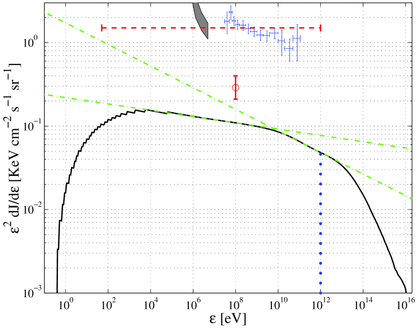
Figure 7: Inverse-Compton spectrum (solid line), contributing $\sim 10\%$ of the EGRET-measured flux (error bars, Sreekumar et al. 1998) and the estimates made in §2.3.1 (dashed line). Below $10\mbox{ MeV}$ the observed flux increases significantly: the shaded region represents results of the Solar Maximum Mission (SMM, Watanabe et al. 1997). The expected contribution from unresolved point sources, based on empirical modeling of the luminosity function of blazars Mukherjee & Chiang (1999), is shown (circle with error bar). Pair production cascade effectively cuts off the spectrum at photon energy $\epsilon\simeq 1\mbox{ TeV}$ (dotted line), slightly enhancing the spectrum below this energy. The approximated spectra, equation (57) and equation (58), are also shown (dash-dotted lines). The step-like feature at low energies is a consequence of the temporal resolution of selected snapshots (and corresponding $\gamma_{\mbox{\tiny min}}$ values).

The inverse-Compton spectrum, predicted by the simulation, extends from the optical band into the far $\gamma$-ray regime, with photon energies in the range $1\mbox{ eV}<\epsilon<10^{4}\mbox{ TeV}$ (Figure 7). However, the high energy tail of this spectrum is modified by photon-photon pair-production interactions, rendering the universe non-transparent for $\epsilon\gtrsim 1\mbox{ TeV}$ photons. Photons of $\epsilon\gtrsim 100\mbox{ TeV}$ thus interact with CMB photons or, at much higher energies, with radio background photons. Lower energy ($1\mbox{ TeV}<\epsilon<100\mbox{ TeV}$) photons interact mainly with the intergalactic infrared (IR) background. The $e^{+}e^{-}$ pairs, produced in such interactions, may inverse-Compton scatter CMB or IR photons, thus initiating a cascade process Nikishov (1962); Gould & Schreder (1967); Protheroe & Stanev (1993). As a result, the $\gtrsim 1\mbox{ TeV}$ spectrum is significantly attenuated, whereas at lower photon energies, piling-up of the cascading photons slightly enhances (flattens) the spectrum.

The resulting spectrum provides roughly equal energy flux per decade in photon energy, in the photon energy range $10\mbox{ keV}\lesssim\epsilon\lesssim 1\mbox{ TeV}$. This flux ranges from $\epsilon^{2}dJ_{\gamma}(\epsilon)/d\epsilon_{\gamma}\simeq 160\mbox{ eV cm}^{-2}\mbox{ s}^{-1}\mbox{ sr}^{-1}$ at $\epsilon=10\mbox{ keV}$, through $100\mbox{ eV cm}^{-2}\mbox{ s}^{-1}\mbox{ sr}^{-1}$ at $\epsilon=1\mbox{ GeV}$, and down to $50\mbox{ eV cm}^{-2}\mbox{ s}^{-1}\mbox{ sr}^{-1}$ at $\epsilon=1\mbox{ TeV}$. The number flux of photons in the energy range $10\mbox{ keV}\lesssim\epsilon\lesssim 1\mbox{ GeV}$ is well approximated by:

$$\frac{dJ_{\gamma}}{d\epsilon_{\gamma}}(\epsilon)\simeq 1.1\times 10^{-14}\left(\frac{\epsilon}{100\mbox{ MeV}}\right)^{-2.04}\left(\mbox{eV cm}^{2}\mbox{ s sr}\right)^{-1}\mbox{ ,}$$ (57)

whereas in the energy range $10\mbox{ GeV}\lesssim\epsilon\lesssim 5\mbox{ TeV}$ the spectrum is slightly steeper and may be approximated, before including the cascade process, by:

$$\frac{dJ_{\gamma}}{d\epsilon_{\gamma}}(\epsilon)\simeq 8.8\times 10^{-19}\left(\frac{\epsilon}{10\mbox{ GeV}}\right)^{-2.13}\left(\mbox{eV cm}^{2}\mbox{ s sr}\right)^{-1}\mbox{ .}$$ (58)

The slope of the resulting spectrum and the energy range over which it extends are in good agreement with the order of magnitude estimates, carried out in §2.3.1. The resulting flux, on the other hand, falls short of the early estimates of equation (19) and equation (20), by a factor $\sim 10$ (Figure 7).

The discrepancy between the above flux, calculated from the simulation, and the flux predicted in §2.3.1, is due to a combination of several factors. First, the temperature reached by the simulation is a factor of $\sim 2.6$ lower than the order-of-magnitude temperature $10^{7}\mbox{ K}$ assumed previously. The thermal energy gain in the epoch examined ($0<z<2$) is thus smaller than the thermal energy used in §2.3.1 by a factor of $\sim 3$. Second, the energy induced by the identified shocks constitutes a fraction $f_{\mbox{\tiny sh}}\sim 2/3$ of the thermal energy gain in the simulation, as opposed to the previous assumption $f_{\mbox{\tiny sh}}=1$. Third, the simulation identifies only approximately half of the shock-induced electron-energy in electrons, that had sufficient time to cool ($\gamma>\gamma_{\mbox{\tiny min}}$), in contrast to the factor $1-\ln{(\gamma_{\mbox{\tiny min}})}/\ln{(\gamma_{\mbox{\tiny max}})}\simeq 2/3$ of §2.3.1, indicating the presence of weak shocks and very recent shocks. Finally, in §2.3.1 we neglected the redshift of the emitted energy, caused by the expansion of the universe, assuming that most the detected radiation was emitted recently ($z<0.5$). However, the energy accumulated by the detected shocks increases almost steadily for $z<2$ (Figure 5, left), such that a significant fraction of the predicted flux originates at high redshifts: only $\sim 40\%$ of this flux was emitted at $z<0.5$. This effect reduces the predicted flux by a factor $\sim 5/3$. Summing up the effects listed above, found from Table 3, yields the discrepancy factor: $3\cdot(3/2)\cdot(4/3)\cdot(5/3)=10$.

5.2 Sky Maps, $\gamma$-ray Sources and Source Number-Counts

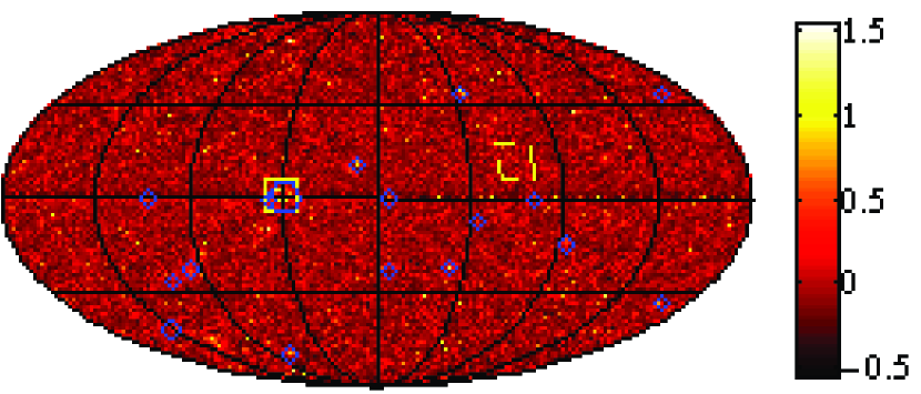
Figure 8: Full $\gamma$-ray sky map at photon energies above $100\mbox{ MeV}$. Color scale represents $\log_{10}\left(J/\bar{J}\right)$, where $\bar{J}=1.1\times 10^{-6}\mbox{ cm}^{-2}\mbox{ s}^{-1}\mbox{ sr}^{-1}$ is the average photon number flux at these energies. Longitudes and latitudes (dark lines) are plotted $45^{\circ}$ apart. Bright contours enclose regions magnified in Figure 9. Blue circles show simulated sources that will be well-resolved by GLAST in photon energies above $1\mbox{ GeV}$ (for $\xi_{e}=0.05$). Angular resolution is $\sim 42^{\prime}$.

By integrating the predicted flux, arriving from different directions, one can construct maps of the simulated $\gamma$-ray sky. Maps of the entire sky (Figure 8) and of two selected regions (Figure 9) are presented in the following. They reveal a globally isotropic picture, with strong local fluctuations, e.g. flux variation over $2$ orders of magnitude at $\sim 1^{\circ}$ resolution and over more than $3$ orders of magnitude at $\sim 5^{\prime}$ resolution. Such maps of the predicted $\gamma$-ray sky can be directly compared to the maps produced by detectors such as EGRET Sreekumar et al. (1998) aboard the CGRO satellite, detectors on board GLAST, planned for launch in 2006, and Čherenkov telescopes such as MAGIC, VERITAS and HESS . Since such devices have finite angular resolution, the simulated maps must be convolved with appropriate filter functions, as demonstrated in Figure 9. The relevant parameters of EGRET, GLAST and MAGIC are summarized in Table 4.

Various $\gamma$-ray sources, of different shapes and sizes, are observed in the simulated maps of the $\gamma$-ray sky. Some of these sources exhibit irregular shapes, revealing the underlying structure of their emitter. Two typical examples, depicted in Figure 9, are strong emission from a semi-spherical source, and weak emission from a filamentary object. Some interesting features of the semi-spherical $\gamma$-ray source are shown in Figure 10. This source is the signature of a nearby rich galaxy cluster, lying $\sim 53\mbox{ Mpc}$ from the simulated observer, at a redshift of $z\simeq 0.012$. The $\gamma$-ray emission from the cluster appears approximately as an elliptic ring, corresponding to a diameter $5-10\mbox{ Mpc}$, surrounding the location of the cluster and indicating the position of its accretion shock. The luminosity has two evident peaks along the circumference of the ring, approximately at the locations of its intersections with two large galaxy filaments. This suggests that the strong emission from these two regions is due to shocked gas, channeled by the filaments into the cluster region. Other galaxy filaments may be responsible for less luminous peaks of emission along the circumference of the ring, on the right hand side of Figure 10 images.

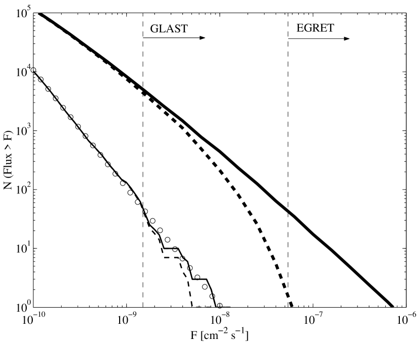
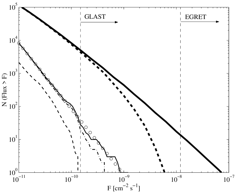
Figure 11: Cumulative all-sky number of $\gamma$-ray sources with observed photon number flux exceeding $F$, for photon energies above $100\mbox{ MeV}$ (left panel) and above $1\mbox{ GeV}$ (right panel). Plotted are the number of all sources (thin solid line) and the number of sources with angular size smaller than the $1\sigma$ photon-arrival spread of EGRET (dash-dotted line) and of GLAST (thin dashed line). Estimates based on the Press-Schechter mass function Waxman & Loeb (2000) predict a higher number of bright sources (thick solid line) and bright sources with angular size $<1^{\circ}$ (thick dashed line). In both energy ranges, the number of the brightest sources as a function of flux is well-approximated by a power law $N(>F)\sim F^{-2}$ (open circles), steeper than the Press-Schechter based estimates $N(>F)\sim F^{-1.38}$. Also plotted are the detection flux thresholds of EGRET and GLAST (vertical dashed lines).

The simulated sky maps produced may be decomposed into discrete $\gamma$-ray sources, yielding number counts of sources above given photon energies (Figure 11). This is performed using a greedy source-identification algorithm devised for the purpose, discussed in Appendix B. The resulting number counts of sources above $100\mbox{ MeV}$ and above $1\mbox{ GeV}$ fall short of the EGRET detection threshold. Our simulation thus predicts that none of the $\sim 60$ unidentified extragalactic EGRET sources Özel & Thompson (1996) can be attributed to intergalactic shock-induced emission. The number-counts are especially sensitive to the fraction of shock-energy transferred to the relativistic electrons. For $\xi_{e}=0.05$ our simulation predicts a few dozen sources detectable by GLAST at both photon energy ranges, among them $16$ well-resolved sources above $1\mbox{ GeV}$ associated with different objects in the sky (see Figure 8). For $\xi_{e}=0.02$, the simulation predicts only one source detectable by GLAST, whereas $\xi_{e}=0.10$ yields more than a hundred GLAST sources, well resolved above $1\mbox{ GeV}$, yet too faint for EGRET detection.

Since our source-identification algorithm was devised for spherical sources, very large, nearby objects tend to be broken down and identified as several separate, weaker ones. This implies that when comparing our source number counts with analytical predictions Waxman & Loeb (2000); Totani & Kitayama (2000), one should impose a threshold on the angular size of the sources. As evident from Figure 11, Our number counts fall short of those of Waxman & Loeb (2000) by a factor of $\sim 6$. This may be explained, at least partially, by the same factors listed above that reduce the simulated diffuse $\gamma$-ray flux compared to the analytic calculation: the lower average temperature of the simulation suggests less hot, massive clusters, and combined with the thermal efficiency of the shocks and the fraction of electrons that had sufficient time to cool, both lower than assumed in the analytical predictions, may account for the discrepancy factor.

6 Discussion

We have studied the $\gamma$–ray emission from intergalactic shock waves, using a hydrodynamic $\Lambda\mbox{CDM}$ cosmological simulation, according to the model proposed by Loeb & Waxman (2000). A simple approach for extracting large-scale shocks from a Lagrangian simulation, based on following entropy changes of single simulated particles, was employed. This method was shown to identify most of the strong (Mach number $M\gtrsim 100$) accretion shocks in the simulation containing a large fraction ($f_{\mbox{\tiny sh}}\sim 2/3$) of the gas thermal-energy gain, although some of the weaker ($M\lesssim 10$) flow or merger shocks might be missed. Relativistic electron populations, Fermi-accelerated by the shocks, were injected into the shocked gas, assuming that a fraction $\xi_{e}=0.05$ of the shock thermal energy was transferred into relativistic electrons. The inverse-Compton radiation, emitted as these electrons scatter CMB photons, was then calculated and integrated over space and time, to yield the radiation detected by an imaginary observer.

This radiation was found to extend from the optical band and into the far $\gamma$-ray regime, containing roughly equal energy flux per decade in photon energy, $\epsilon^{2}[dJ_{\gamma}(\epsilon)/d\epsilon_{\gamma}]\simeq 50-160\mbox{ eV cm}^{-2}\mbox{ s}^{-1}\mbox{ sr}^{-1}$, in the photon energy range $10\mbox{ keV}\lesssim\epsilon\lesssim 1\mbox{ TeV}$. The calculated spectral slope, $dJ/d\epsilon\sim\epsilon^{-2.04}$ for $10\mbox{ keV}\lesssim\epsilon\lesssim 1\mbox{ GeV}$ and $dJ/d\epsilon\sim\epsilon^{-2.13}$ for $10\mbox{ GeV}\lesssim\epsilon\lesssim 5\mbox{ TeV}$ (before accounting for photon-photon pair-production cascade), is consistent with the predictions of Loeb & Waxman (2000) and with the EGRET observations. The energy flux constitutes $\sim 10\%$ of the EGRB flux, or up to $\sim 15\%$ of the EGRB flux after subtracting the expected contribution from unresolved point sources based on empirical modeling of the luminosity function of blazars Mukherjee & Chiang (1999).

The simulated $\gamma$-ray sources, mostly spheroidal halos associated with large-scale structure, fall short of the EGRET detection threshold, thus producing a diffuse background. Hence, the simulation predicts that none of the $\sim 60$ unidentified EGRET extragalactic $\gamma$-ray sources can be attributed to intergalactic shock-induced radiation. Several sources do fall within the detection range of GLAST, planned for launch in 2006, provided that $\xi_{e}\gtrsim 0.03$. The number of detectable sources is sensitive to the fraction of shock-energy transferred to the relativistic electrons: For $\xi_{e}=0.05$ we find several dozen sources detectable by GLAST, among them $16$ well-resolved sources (see Figures 8, 11), whereas $\xi_{e}=0.10$ is still insufficient for EGRET detection, but leads to more than a hundred well-resolved GLAST $\gamma$-ray sources. Such sources could be identified as emission from intergalactic shock-accelerated electrons, by association with large-scale structure, a characteristic $dJ/d\epsilon\sim\epsilon^{-2}$ spectrum, extending up to the far $\gamma$-ray regime, and a low cutoff at photon energy $\epsilon_{\mbox{\tiny min}}\simeq 5\left(t/10^{9}\mbox{ yr}\right)^{-2}\mbox{ keV}$, caused by low-energy electrons not having sufficient time to cool during the lifetime $t$ of the source. Detection of intergalactic shock-induced $\gamma$-ray sources may be used to calibrate $\xi_{e}$, once their temperature has been determined. The shock-induced $\gamma$-ray emission, a first direct tracer of the warm-hot IGM ($10^{5}\mbox{ K}\lesssim T\lesssim 10^{7}\mbox{ K}$), may thus be used to determine the baryon density in the present-day universe.

We have examined the $\gamma$-ray signature of a nearby simulated rich galaxy cluster, lying at a redshift $z\simeq 0.012$. An elliptic emission ring of a diameter corresponding to $5-10\mbox{ Mpc}$ surrounds the cluster, tracing the location of its accretion shock (see Figures 9, 10). The luminosity peaks along the circumference of this ring, probably at the locations of intersections with galaxy filaments, channeling gas into the cluster region. Similar features should be detected by GLAST or by the MAGIC telescope in nearby rich galaxy clusters, at photon energies above $10\mbox{ GeV}$, and by VERITAS and HESS above $200\mbox{ GeV}$, if the background signal is assumed flat. A ring-like feature resembling the simulated emission should thus be detected in such galaxy clusters lying at redshifts $z\lesssim 0.01$, whereas the brightest regions of emission along the circumference of the ring could be detected in clusters with redshifts up to $z\simeq 0.025$. These bright regions of emission lie above the background signal and should be detected at redshifts $z\lesssim 0.015$ even for $\xi_{e}=0.02$, whereas $\xi_{e}=0.10$ will enable the detection of the emission ring itself at similar redshifts. Detection of such a ring will enable a direct study of the cluster accretion shock, as well as establish the validity of our model. Detected bright regions along the circumference of such a ring may be tested to comply with data regarding a nearby galaxy filament and be used to measure the density and velocity of the untraced gas in such a filament.

As mentioned above, our algorithm for extracting shocks succeeded in capturing strong shocks, but missed some of the weaker ($M\lesssim 10$) ones. Accounting for these weak shocks could only have a minute effect on the predicted diffuse $\gamma$-ray radiation, since most ($\sim 2/3$) of the thermal energy has been identified in strong shocks and because the steep spectrum of electrons accelerated by weak shocks reduces their $\gamma$-ray efficiency. Weak shocks could, however, increase the $\gamma$-ray brightness of nearby structures such as galaxy clusters encompassing ongoing merger processes, mainly in low photon energies, slightly altering the appearance of their inner regions and enhancing the predicted source number counts.

In our work we have neglected the radiation resulting from the protons accelerated in the intergalactic shocks. These protons lead to $\gamma$-ray emission as they scatter off thermal protons to produce pions, most of the $\gamma$-ray flux originating from $\pi^{0}$ decay. Even with a large proton-to-electron energy ratio $\eta$, the radiation resulting from the relativistic protons is, on average, negligible compared to the emission from electrons. Only in the densest ($n>10^{-3}\mbox{ cm}^{-3}$) regions in the cores of clusters, the relativistic protons may alter the $\gamma$-ray spectrum. This effect may make the cores of clusters even brighter $\gamma$-ray sources, provided that is not eliminated by diffusion of the relativistic protons out of the over-dense regions. For the values of $\xi_{e}$ and $\eta$ discussed above, the relativistic protons are dynamically significant and play an important role in shock dynamics and in particle acceleration. These effects, possibly detected in the radio spectra of some supernovae remnants, are small Reynolds & Ellison (1992), suggesting that the linear approach adopted in this paper is sufficiently adequate.

One can confirm that at least part of the EGRB is associated with the large-scale structure of the universe, by cross-correlating $\gamma$-ray maps with other sources that trace the same structure, such as galaxies, X-ray gas and the Sunyaev-Zel’dovich effect. The intergalactic shock-origin of $\gamma$-ray radiation may be verified by cross-correlating the EGRB with radio maps, partly attributed to synchrotron emission from the same shock-accelerated electrons. The synchrotron radio radiation is sub-dominant to the CMB, although its strong fluctuations on sub-degree scales were shown to contaminate CMB fluctuations at low ($\nu\lesssim 10\mbox{ GHz}$) frequencies Waxman & Loeb (2000). Detection of a radio – $\gamma$-ray cross-correlation signal from nearby clusters may be used to measure the intergalactic magnetic field. The auto-correlation of inverse-Compton or synchrotron radiation, as well as their cross-correlation, may be calculated directly from our simulation.

A study of the shock-induced component of the extragalactic radiation, combined with a calculation of shock-induced emission according to cosmological simulations as described in this paper, may provide an important test of structure-formation models. Angular statistics of the $\gamma$-ray radiation, both on its own and cross-correlated with other sources, may be measured and compared to the predictions of such simulations. This will enable a study of the large-scale structure of the universe, and provide insight to the structure-formation process itself. We plan to apply the tools, developed in this research, to other cosmological simulations, including high-resolution simulations incorporating radiative cooling processes and supernovae feedback (e.g. Springel & Hernquist 2002b). Such research will permit an extensive study of shock-induced radiation, in the framework of various cosmological structure-formation models. Other physical phenomena, such as the acceleration of cosmic-rays by intergalactic shocks, may thus be investigated as well.

Order-of-magnitude estimates, presented in §2.3.1, predict an inverse-Compton flux higher by a factor of $\sim 10$ than obtained from the simulation we have studied. This is primarily attributable to the lower present-day temperature reached by the simulation, $T_{0}\simeq 4\times 10^{6}\mbox{ K}$, and to its slower heating-rate, which seem to comply with other recent simulations. Our simulation neglected radiative cooling, suffered from relatively low mass resolution ($\sim 10^{11}M_{\odot}$), and did not include feedback from supernovae explosions, photo-heating the surrounding matter. The effect of radiative cooling on the accretion shocks is expected to be small, as cooling is efficient in hot, dense regions, beyond these shocks, and in cold, dilute regions, where the temperatures are low to begin with. Cooling should have a non-negligible effect on merger and flow shocks, but since these are much weaker than the accretion shocks, this should not significantly alter our results. In order to examine the sensitivity of our results to the low resolution of the simulation, a preliminary check of a similar adiabatic $\Lambda$CDM simulation, with identical cosmological parameters but with eight times the mass resolution, was carried out, exhibiting no substantial difference from the results presented above. Outflows from galaxies (due to starburst or quasar activities) could also result in shock acceleration of relativistic electrons as they impact on the surrounding IGM. At the same time, preheating of the collapsing matter by, for example, supernovae, may lead to weaker, cooler shocks, as recently pointed out by Totani & Inoue (2001), and thus result in softer, weaker photon emission. However, Davé et al. (2001b) find that the luminosity-temperature relation for galaxy clusters, which originally motivated the addition of preheating to structure formation models, may in fact be attributed to radiative cooling. Therefore, preheating may not have played an important role in structure formation after all, and thus have little effect on our results.

Note added in proof: Recently, Scharf & Mukherjee (2002) have pointed out a possible association of $\gamma$-ray emission with the locations of galaxy clusters, by cross-correlating high Galactic latitude EGRET data with Abell clusters. The correlation signal, identified at a confidence level of $3\sigma$, is broadly consistent with the extended emission and with the source number counts discussed above, suggesting good prospects for the detection of extended $\gamma$-ray emission from clusters by future observations.

Appendix A Integration Parameters

In order to perform the space-time integration schemes described in section 4.3.2, one must find the redshift dependence of several parameters: the time that elapsed between redshift $z$ and the present, the coordinate distance, traversed by a photon in that time, and the minimal Lorentz factor of electrons that lost a significant fraction of their energy since redshift $z$. Formulae for these parameters are provided below.

Using the FRW equations, we find that the time that elapsed between redshift $z$ and the present is given by:

$$\Delta t=t_{0}-t(z)=\int_{R(z)}^{R(z=0)}\frac{1}{\dot{R}}\,dR=H_{0}^{-1}\int_{0}^{z}\frac{1}{(1+z)h(z)}\,dz\mbox{ ,}$$ (A1)

where $h(z)\equiv H(z)/H_{0}$. The coordinate distance traversed by a photon in that period is given by:

$$r=g\left[\int_{R(z)}^{R(z=0)}\frac{c}{\dot{R}R}\,dR\right]=g\left[\frac{c}{R_{0}H_{0}}\int_{0}^{z}h(z)^{-1}\,dz\right]\mbox{ ,}$$ (A2)

where $g(x)$ is a function of the curvature $k$, defined by:

$$g(x)\equiv\cases{\sin{(x)}&for $k=1$ ;\cr x&for $k=0$ ;\cr\sinh{(x)}&for $k=-1$ .\cr}$$ (A3)

For our $\Lambda\mbox{CDM}$ model, where $\Omega_{\Lambda}+\Omega_{M}=1$ and $h(z)=\sqrt{\Omega_{\Lambda}+(1+z)^{3}\Omega_{M}}$, the above equations are solved to give:

$$\Delta t=\frac{2}{3H_{0}\sqrt{\Omega_{\Lambda}}}\ln\left[{\frac{(1+\sqrt{\Omega_{\Lambda}})(1+z)^{3/2}}{\sqrt{\Omega_{\Lambda}}+\sqrt{\Omega_{M}(1+z)^{3}+\Omega_{\Lambda}}}}\right]\mbox{ ,}$$ (A4)

and:

$$r=\frac{c}{3R_{0}H_{0}}\frac{{(-1)}^{2/3}}{\Omega_{M}^{1/3}\Omega_{\Lambda}^{1/6}}\mbox{ }\beta\left[\frac{1}{\Omega_{\Lambda}},1+\frac{\Omega_{M}}{\Omega_{\Lambda}}\left(1+z\right)^{3},\frac{1}{2},\frac{1}{3}\right]\mbox{ ,}$$ (A5)

where $\beta$ is the incomplete beta function, defined by:

$$\beta\left[t_{1},t_{2},a,b\right]\equiv\int_{t_{1}}^{t_{2}}t^{a-1}\left(1-t\right)^{b-1}\,dt\mbox{ .}$$ (A6)

In a similar fashion, we find the redshift dependence of $\gamma_{\mbox{\tiny min}}(z,p)$, the minimal Lorentz factor of an electron, that looses a fraction $p$ of its energy between redshift $z$ and today by inverse-Compton scattering. This parameter, which determines the low cutoff of the resulting spectrum, is given by:

$$\gamma_{\mbox{\tiny min}}(z,p)=\frac{p}{(1-p)}\frac{3m_{e}cH_{0}}{4\sigma_{T}u_{\mbox{\tiny CMB}}(z=0)}\left[\int_{0}^{z}\frac{(1+z)^{3}}{h(z)}\,dz\right]^{-1}\mbox{ ,}$$ (A7)

which for our $\Lambda\mbox{CDM}$ model can be solved to give:

$$\gamma_{\mbox{\tiny min}}(z,p) = 400h_{67}\frac{p}{(1-p)}\Omega_{M}/\left\{(1+z)h(z)-1+\sqrt{\Omega_{\Lambda}}F\left(\frac{\Omega_{M}}{\Omega_{\Lambda}}\right)\right.$$ (A8)

$$- \left.(1+z)\Omega_{\Lambda}F\left[(1+z)^{3}\frac{\Omega_{M}}{\Omega_{\Lambda}}\right]\right\}\mbox{ ,}$$

where $F(x)$ is the hyper-geometric function ${}_{2}F_{1}\left(\frac{1}{3},\frac{1}{2},\frac{4}{3},-x\right)$, defined by ${}_{2}F_{1}\left(\frac{1}{3},\frac{1}{2},\frac{4}{3},-x\right)\equiv\sum_{k=0}^{\infty}\left(\frac{1}{3}\right)_{k}\left(\frac{1}{2}\right)_{k}(-x)^{k}/\left(\frac{4}{3}\right)_{k}k!$.

The redshift dependence of the parameters calculated above, also demonstrating the criteria for snapshot selection (simulation-box light-crossing time), is depicted in Figure 12.

Appendix B Source Identification Algorithm

In order to count discrete $\gamma$-ray sources, predicted by the simulation, we have devised a greedy algorithm for extracting point sources from a sky map. This algorithm is used to isolate such sources, determine their location and flux, and measure their angular size. The algorithm operates iteratively, identifying sources and removing them from the map, until the contrast of the remaining map is smaller than some imposed threshold (of order $2$). At each iteration, the algorithm searches for the brightest point in the sky, and attempts to identify the brightest source associated with it. Our candidate for the source is assumed to have its kernel positioned about this bright point. We determine the area around the kernel, associated with the source by examining concentric rings about the kernel and adding them to the ’growing’ source. This accumulation process lasts as long as the flux within such a ring is sufficiently higher than the background, throughout its circumference, and yet monotonically decreasing, at least at one point along the circumference. Once the entire source has been identified, the flux associated with it is carefully removed from the map. The flux subtracted from each ring is determined according to the faintest point along its circumference, in order to prevent upsetting adjacent sources.

The source number counts produced by the algorithm were analyzed in section 5.2, with respect to the experimental devices EGRET and GLAST. In order to do so, algorithm parameters were tuned to mimic the source identification process, used to analyze the experimental data. Hence, the angular resolution of the analyzed sky maps was set to match the point-source resolution of the experimental devices, and the angular size of each source was compared to the photon-position error of each experiment, as illustrated in Figure 11.

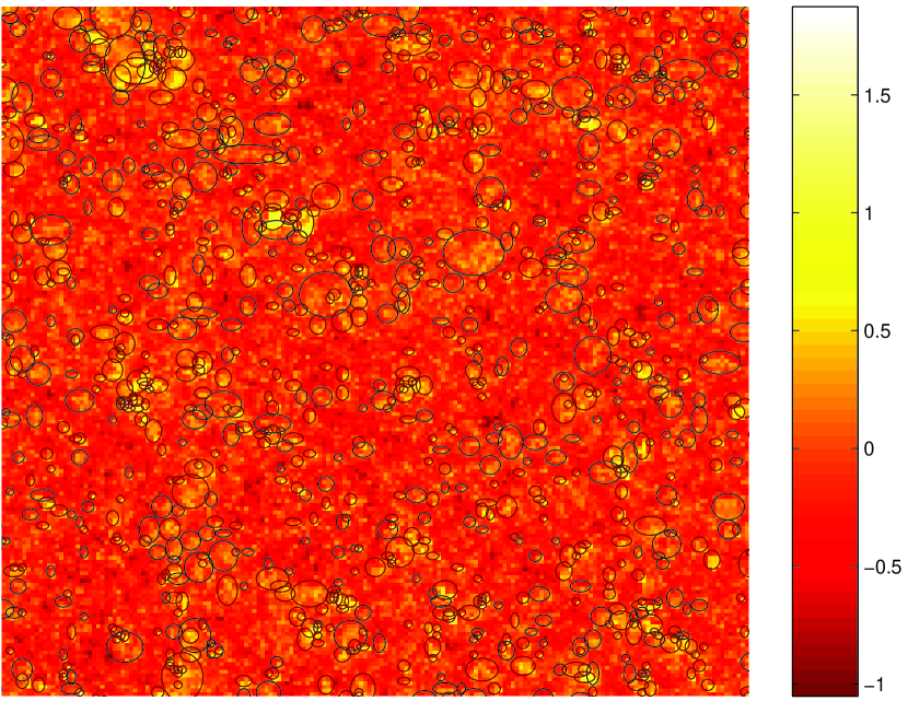
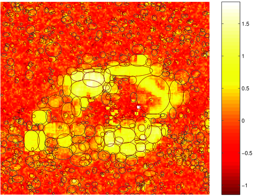
Figure 13: Results of the source-identification algorithm, when applied to two regions in the $\gamma$-ray sky. Both images are of angular size $16^{\circ}\times 16^{\circ}$, and are similar (but not identical) to those presented in Figure 9. Color scale is identical to the one shown in Figure 9.

Figure 13 demonstrates the results of the algorithm, when applied to two regions in the simulated $\gamma$-ray sky. The sky maps displayed in this paper were produced by approximating the source, associated with each SPH particle, as a rectangle in $\theta-\phi$ space. The resulting image of a source, produced by a single SPH particle, thus assumes a trapezoidal-like shape when mapped to a surface, centered at the source. Similarly, The concentric ’rings’ discussed above are in fact rectangles in $\theta-\phi$ space. The identified sources are thus depicted in Figure 13 as ellipses instead of rectangles for illustrative purposes only.

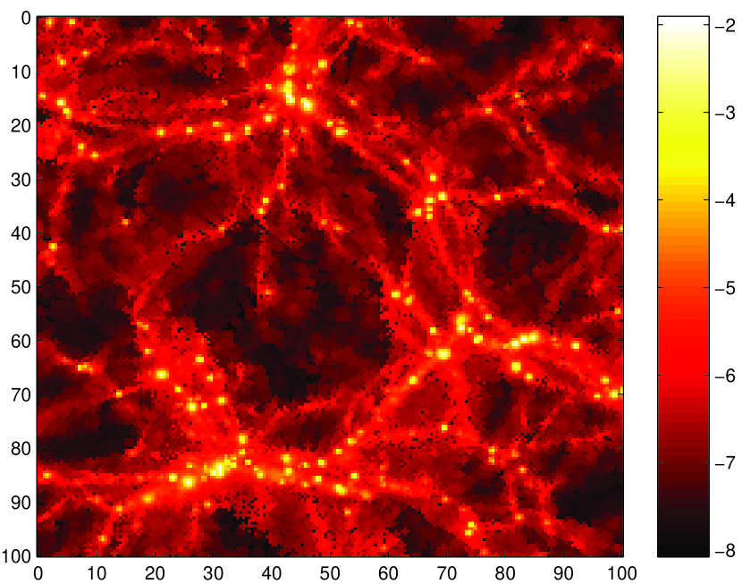
Figure 1: Imaging a partial slice of the simulation box at $z=0$. Width and height are $100\mbox{ Mpc}$, depth is $10\mbox{ Mpc}$.
left: Maximal baryon number density through the slice. Color scale: $\log_{10}{\left(n\left[\mbox{cm}^{-3}\right]\right)}$.
right: Maximal temperature through the slice. Color scale: $\log_{10}{\left(T\left[\mbox{K}\right]\right)}$.

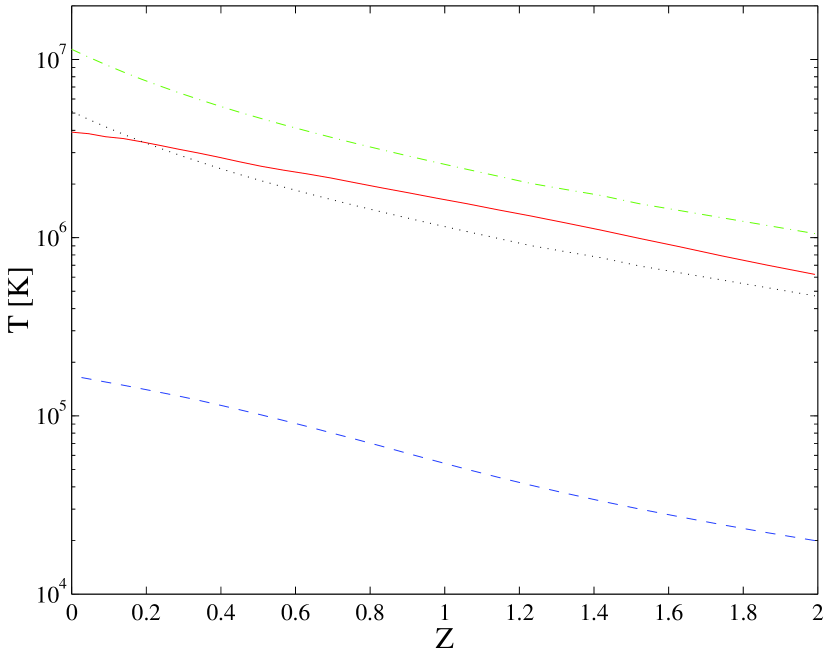
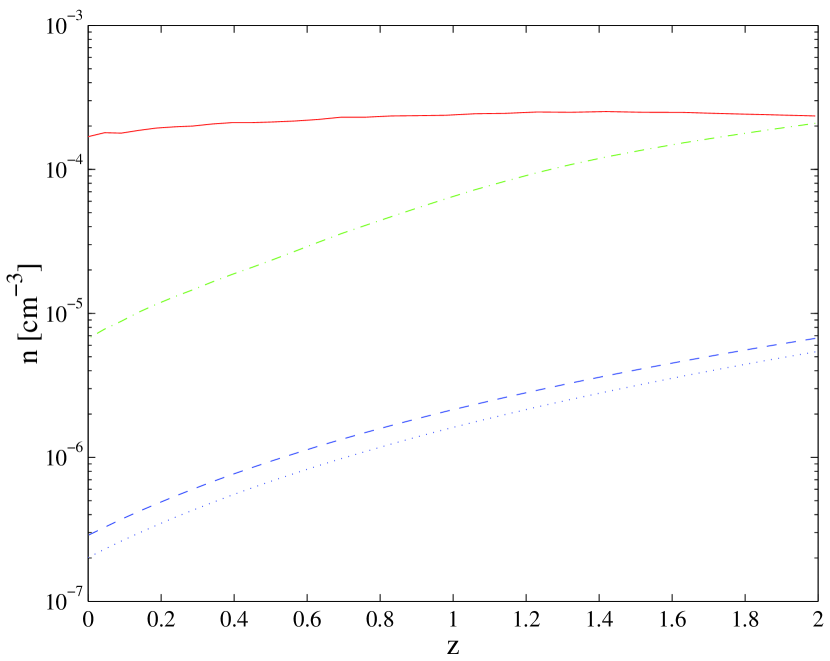
Figure 2: Thermodynamic evolution of the simulated universe at recent epochs.
left: The temperature averaged over mass ($\rho^{1}$ averaging, solid line) and over volume ($\rho^{0}$ averaging, dashed line). The mass averaged temperature according to the approximation of equation (5) is plotted as well, for $k=1$ (as assumed in §2.1, dash-dotted line) and for $k=0.67$ (best fit to data, dotted line).
right: Baryon number density averaged over mass (solid line), over volume (dashed line) and over temperature (dash-dotted line). The volume-averaged density overshoots its predicted value ($\sim\left[1+z\right]^{3}$, dotted line), probably due to limited simulation resolution in dilute regions.

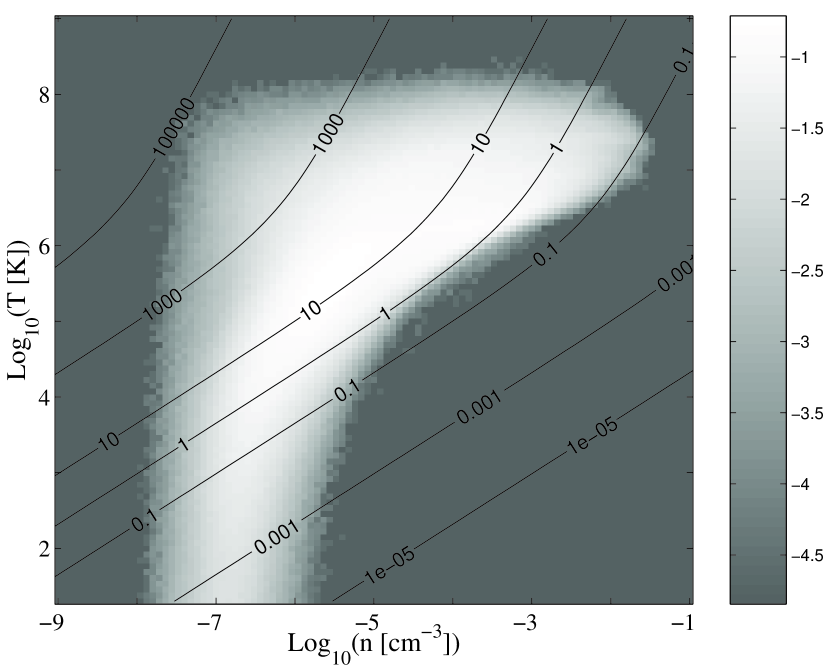
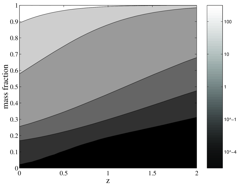
Figure 3: Radiative cooling of the simulated gas.
left: Mass distribution at $z=0$ in the phase space of temperature and baryon number density. Gray-scale: the logarithm (base $10$) of the mass fraction $m_{\mbox{\tiny tot}}^{-1}\Delta m/\left[\Delta\log_{10}(T)\cdot\Delta\log_{10}(n)\right]$. Superimposed black contours denote the cooling time $t_{\mbox{\tiny cool}}$ due to Bremsstrahlung and line emission Peacock & Heavens (1990), normalized to the Hubble time $t_{\mbox{\tiny H}}$.
right: Mass fraction of particles with various normalized cooling times in different epochs. Gray scale: $t_{\mbox{\tiny cool}}/t_{\mbox{\tiny H}}(z)$.

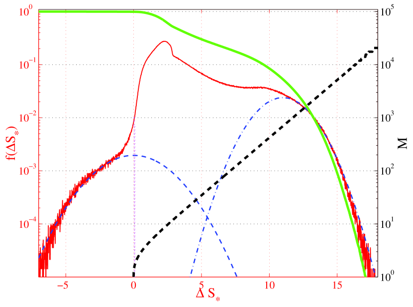
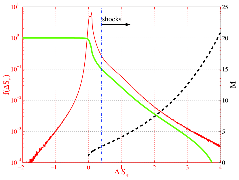
Figure 4: Statistics of normalized entropy-change, $\Delta S_{*}$, accumulated by simulated particles.
Plotted are the mass fraction $f(\Delta S_{*}^{\prime})=m_{\mbox{\tiny tot}}^{-1}dm(\Delta S_{*}^{\prime})/d\Delta S_{*}$ (thin solid line), integrated mass fraction $m_{\mbox{\tiny tot}}^{-1}m(\Delta S_{*}>\Delta S_{*}^{\prime})=\int_{\Delta S_{*}^{\prime}}^{\infty}f(\Delta S_{*})\,d\Delta S_{*}$ (thick solid line) and the shock Mach number, $M$, corresponding to positive $\Delta S_{*}$ values (thick dashed line, right axes).
left: Total entropy accumulated in the recent epoch, $\Delta S_{*}=S_{*}(z=0)-S_{*}(z=2)$. The distribution of negative $\Delta S_{*}$ values, approximated by a normal distribution (thin dashed line), is likely due to numerical errors, leaving behind a narrower distribution (well-deconvolved up to $\Delta S_{*}\sim 1$, dotted line). High positive $\Delta S_{*}$ values are also well-fitted by a normal distribution (dash-dotted line).
right: Average $\Delta S_{*}$ between two consecutive snapshots. A minimal threshold for shock detection (dash-dotted line) was imposed at $\Delta S_{*}=0.4$, where estimated mass fraction due to numerical noise is $f(\Delta S_{*})\sim 1\%$ (according to negative $\Delta S_{*}$ distribution). On average, $10\%$ of the gas experiences higher entropy increases between consecutive snapshots.

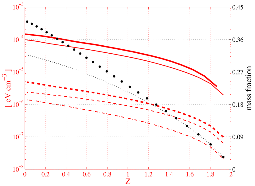
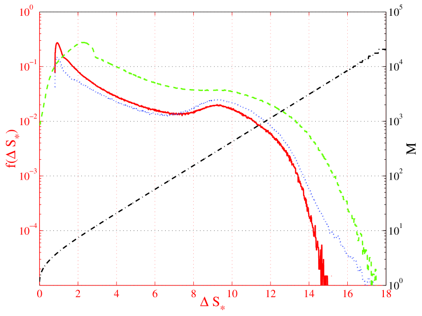
Figure 5: Results of shock extraction between $z=2$ and $z=0$.
left: Redshift dependence of the comoving energy densities (left axes), accumulated since $z=2$, of: the simulated gas (thick solid line), the identified shocks (thin solid line), shock–accelerated electron population assuming $\xi_{e}=0.05$ (thick dashed line), electrons within the relevant energy range $\gamma_{\mbox{\tiny min}}<\gamma<\gamma_{\mbox{\tiny max}}$ (thin dashed line) and the redshifted inverse-Compton radiation reaching an observer today (dash-dotted line). Also shown (right axes) are the fraction of the mass that was shocked at least once since $z=2$ (thin dotted line), and the fraction of the mass processed by shocks ($n$ shocks experienced by the same particle counted as $n$ times its mass, thick dotted line).
right: Mass fraction $f(\Delta S_{*})$ with entropy change $\Delta S_{*}$ accumulated between $z=2$ and $z=0$, for all SPH particles before shock extraction (dashed line), among the particles identified as shocked (solid line), and among these particles before multiple shocks experienced by the particles were separated (dotted line). Also shown (right axes) is the Mach number $M$ corresponding to $\Delta S_{*}$ (dash-dotted line).

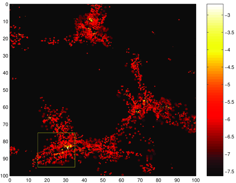
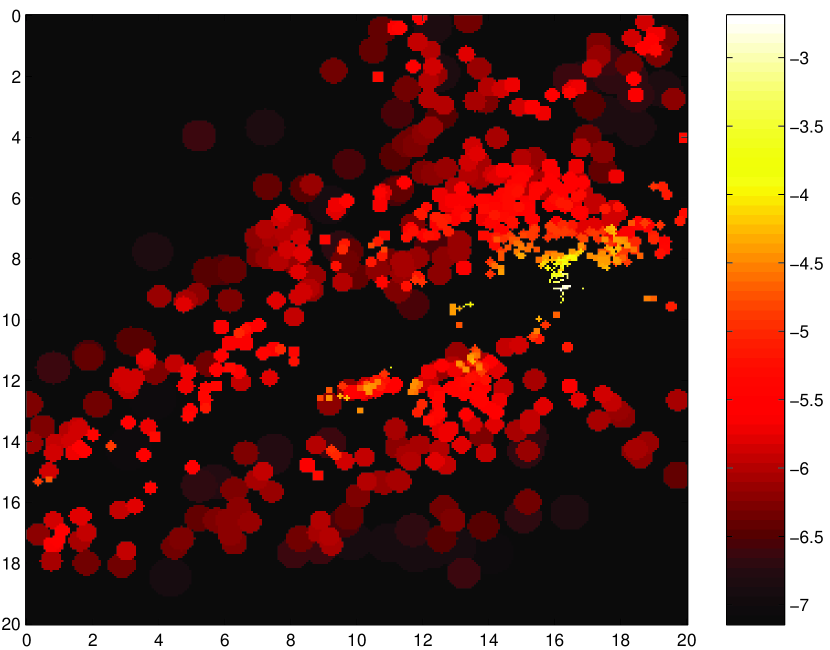
Figure 6: The gas shocked between two consecutive snapshots, taken at $z=0.14$ and at $z=0.09$. Color scale shows the maximal baryon number density through a slice of the simulation box, in $log_{10}(n\left[\mbox{cm}^{-3}\right])$.
left: The same slice as shown in Figure 1, with dimensions $100\mbox{ Mpc}\times 100\mbox{ Mpc}\times 10\mbox{ Mpc}$.
right: Enlarged region in the left image, marked there by a bright square, with dimensions $20\mbox{ Mpc}\times 20\mbox{ Mpc}\times 5\mbox{ Mpc}$.

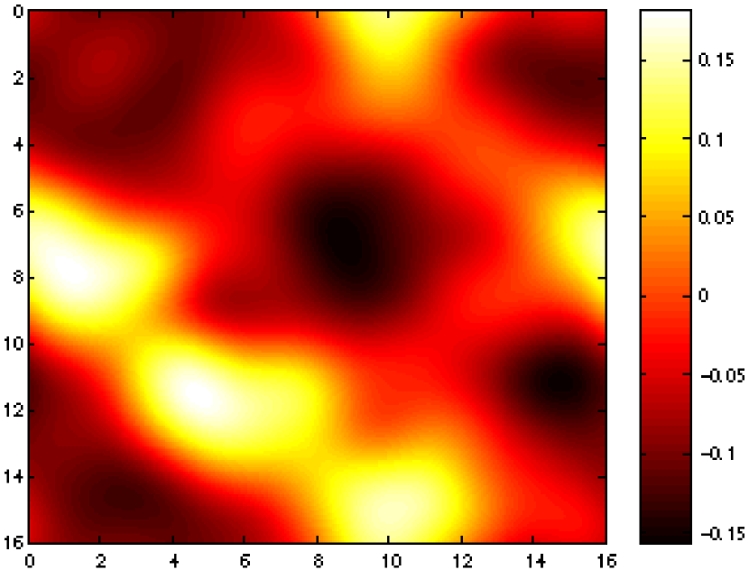
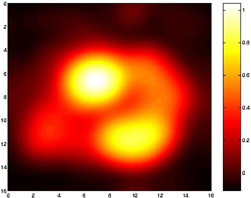
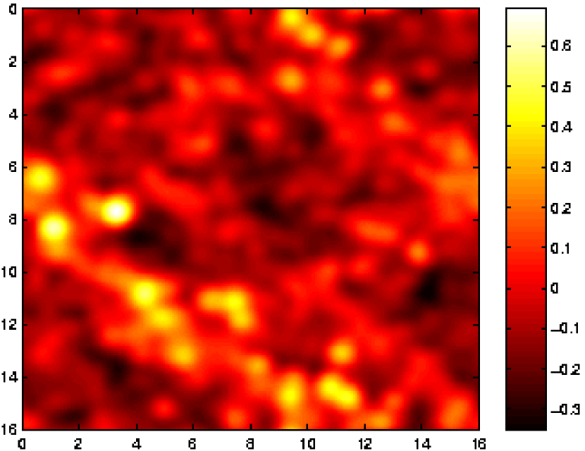
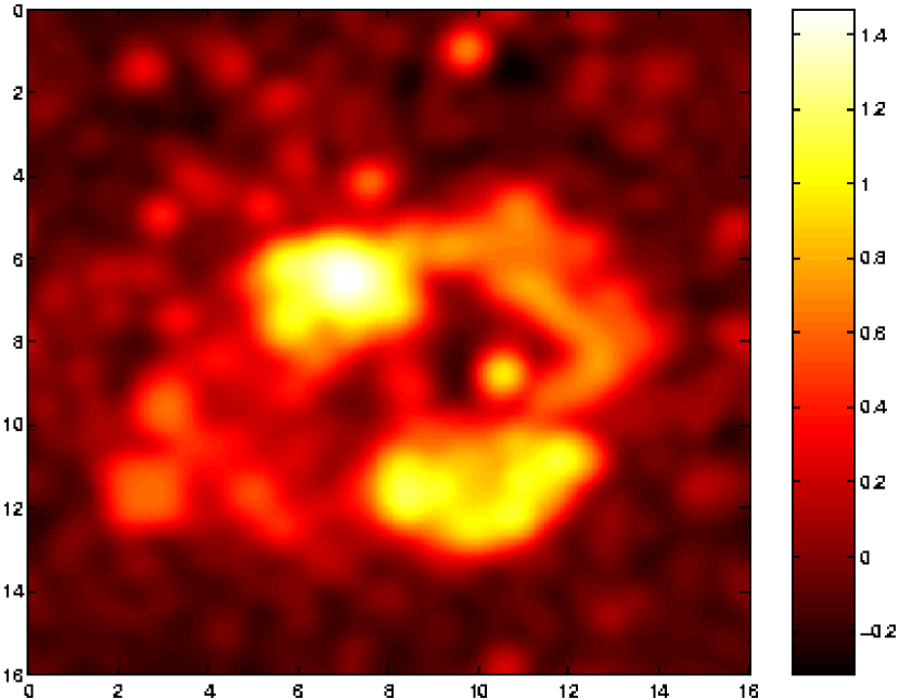
Figure 9: Photon number flux above $1\mbox{ GeV}$ from two $16^{\circ}\times 16^{\circ}$ regions in the sky, marked in Figure 8 by dashed (left images) and solid (right images) bright contours. Images are convolved with Gaussian filter functions, simulating photon angular spread of standard deviation $1.5^{\circ}$ (for EGRET, upper images) and $0.42^{\circ}$ (for GLAST, bottom images). Color scale represents $\log_{10}\left(J/\bar{J}\right)$, where $\bar{J}=9.9\times 10^{-8}\mbox{ cm}^{-2}\mbox{ s}^{-1}\mbox{ sr}^{-1}$ is the average photon number flux above $1\mbox{ GeV}$.

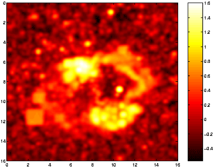
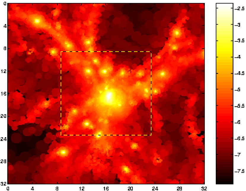
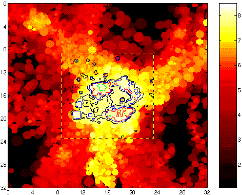
Figure 10: Emission from a nearby rich galaxy cluster.
upper, left: Photon number flux above $10\mbox{ GeV}$ from the $16^{\circ}\times 16^{\circ}$ region shown in Figure 9 (right images). The image is convolved with a Gaussian filter function of standard deviation $0.2^{\circ}$, the expected angular resolution of MAGIC in these energies. Color scale: $\log_{10}\left(J/\bar{J}\right)$, where $\bar{J}=8.2\times 10^{-9}\mbox{ cm}^{-2}\mbox{ s}^{-1}\mbox{ sr}^{-1}$ is the average photon number flux above $10\mbox{ GeV}$.
upper, right: Maximal baryon number density through a thick slice of the simulation box at $z=0$, showing a rich galaxy cluster and connected galaxy filaments. The dashed frame marks the central $\sim 15\mbox{ Mpc}\times 15\mbox{ Mpc}$ region, the emission from which is shown in the upper left image. The slice, of dimensions $32\mbox{ Mpc}\times 32\mbox{ Mpc}\times 8\mbox{ Mpc}$, is oriented perpendicular to the line of sight, with its center located $53\mbox{ Mpc}$ ($z\simeq 0.012$) from the observer. Color scale: $\log_{10}(n\left[\mbox{cm}^{-3}\right])$.
bottom: Maximal temperature through the slice. Color scale: $\log_{10}(T\left[\mbox{K}\right])$. Contours trace lines of constant number flux above $10\mbox{ GeV}$, higher than the average flux in this energy range by a factor ranging from 1.7 (black lines) to 22 (green lines).

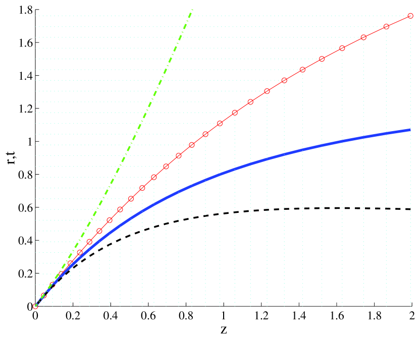
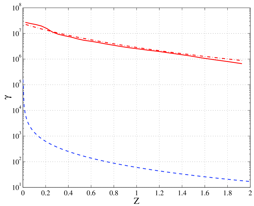
Figure 12: Redshift dependence of the parameters, required for EGRB integration.
left: Coordinate distance ($rR_{0}$, thin solid line) between a source emitting a photon at redshift $z$ and an observer detecting the photon today (in $10^{10}\mbox{ ly}$ units), the angular diameter distance ($rR_{0}/\left[1+z\right]$, dashed line) and the luminosity distance ($rR_{0}\left[1+z\right]$, dash-dotted line) between them. The time that elapsed between emission and detection is given in $10^{10}\mbox{ yr}$ units (thick solid line). Circles and dotted lines illustrate the choice of simulation snapshots examined, separated by the comoving simulation-box light-crossing time.
right: Minimal Lorentz factor of electrons, emitting at least half their energy between redshift $z$ and the present (dashed line), and maximal Lorentz factor reached by the shocked gas according to the simulation (solid line) and according to equation (12) (dash-dotted line), where a post-shock magnetic field of magnitude $B=0.1\mbox{ }\mu\mbox{G}$ was assumed.

Table 1: Parameters of the cosmological model and linear structure formation theory.

Parameter	Meaning	Value
$h$	Hubble parameter	0.67
$k$	Curvature	0
$\Omega_{M}$	Matter energy density	0.3
$\Omega_{DM}$	Dark matter energy density	0.26
$\Omega_{B}$	Baryon energy density	0.04
$\Omega_{\Lambda}$	Vacuum energy density	0.7
$\chi$	Hydrogen mass fraction	0.76
$n$	Fluctuation spectrum slope	1
$\sigma_{8}$	Spectrum normalization	0.9
$z_{\mbox{\tiny start}}$	Starting redshift for the simulation	50

Table 2: Code parameters of the simulation.

Parameter	Meaning	Value
$L_{\mbox{\tiny com}}R(t_{0})$	Simulation box comoving length	$134h^{-1}\mbox{ Mpc}\simeq 200\mbox{ Mpc}$
$N_{\mbox{\tiny DM}}$	Number of dark matter particles	$224^{3}\simeq 11\times 10^{6}$
$M_{\mbox{\tiny DM}}$	Mass of a dark matter particle	$2.3\times 10^{10}\mbox{ M}_{\odot}$
$N_{\mbox{\tiny SPH}}$	Number of gas (SPH) particles	$224^{3}\simeq 11\times 10^{6}$
$M_{\mbox{\tiny SPH}}$	Mass of an SPH particle	$3.55\times 10^{9}\mbox{ M}_{\odot}$
$h_{\mbox{\tiny min}}$	Minimal SPH softening	$6h^{-1}\mbox{ kpc}\simeq 9\mbox{ kpc}$
$N_{s}$	Number of SPH neighbors in kernel	$32$
$M_{\mbox{\tiny res}}$	Minimal Mass Resolution	$\sim 10^{11}\mbox{ M}_{\odot}$
$S_{G}R(t_{0})$	Gravitational softening	$25h^{-1}\mbox{ kpc}\simeq 37\mbox{ kpc}$

Table 3: Comoving energy density $u_{\mbox{\tiny com}}$ of various simulated components.

Parameter	Component	$u_{\mbox{\tiny com}}\left[\mbox{eV cm}^{-3}\right]$
$u_{i}$	gas, at $z=2$	$2.77\times 10^{-5}$
$u_{f}$	gas, at $z=0$	$1.72\times 10^{-4}$
$\Delta u=u_{f}-u_{i}$	gain of gas during $0<z<2$	$1.44\times 10^{-4}$
$u_{\mbox{\tiny sh}}$	detected shocks	$9.62\times 10^{-5}$
$u_{e}$	accelerated electrons ($\xi_{e}=0.05$)	$4.81\times 10^{-6}$
$u_{e}(\gamma_{\mbox{\tiny min}}<\gamma_{e}<\gamma_{\mbox{\tiny max}})$	electrons with $\gamma_{\mbox{\tiny min}}<\gamma_{e}<\gamma_{\mbox{\tiny max}}$	$2.34\times 10^{-6}$
$u_{\gamma}$	radiation, redshifted	$1.40\times 10^{-6}$

Table 4: Parameters of EGRET and of the conceptual designs of GLAST and of MAGIC.

Parameter	Photon Energy	EGRET	GLAST	MAGIC
		(one year all-sky)	(one year all-sky)	($50$ hours)
Point source	$E>100\mbox{ MeV}$	$5.4\times 10^{-8}$	$1.5\times 10^{-9}$	—
– sensitivity	$E>1\mbox{ GeV}$	$1.2\times 10^{-8}$	$1.5\times 10^{-10}$	—
$\left[\mbox{cm}^{-2}\mbox{ s}^{-1}\right]$	$E>10\mbox{ GeV}$	—	$1.0\times 10^{-10}$	$1.0\times 10^{-10}$
Photon –	$E>100\mbox{ MeV}$	$5.6^{\circ}$	$2.5^{\circ}$	—
position –	$E>1\mbox{ GeV}$	$1.5^{\circ}$	$0.42^{\circ}$	—
error ($1\mbox{ }\sigma$)	$E>10\mbox{ GeV}$	—	$0.1^{\circ}$	$0.2^{\circ}$

References

- Achterberg et al. (1994) Achterberg, A., Blandford, R. D., & Reynolds, S. P. 1994, A&A, 351, 330
- Aharonian & Atoyan (1999) Aharonian, F. A. & Atoyan, A. M. 1999, A&A, 281, 220
- Baring et al. (1999) Baring, M. G., Ellison, D. C., Reynolds, S. P., Grenier, I. A., & Goret, P. 1999, ApJ, 513, 311
- Barnes & Hut (1986) Barnes, J. & Hut, P. 1986, Nature, 324, 446
- Barwick et al. (1998) Barwick, S. W. et al. 1998, ApJ, 498, 779
- Blandford & Eichler (1987) Blandford, R. & Eichler, D. 1987, Phys. Rep., 154, 1
- Cargill & Papadopoulos (1988) Cargill, P. J. & Papadopoulos, K. 1988, ApJ, 329, L29
- Cen & Ostriker (1999) Cen, R. & Ostriker, P. 1999, ApJ, 514, 1
- Croft et al. (2001) Croft, R. A. C., Di Matteo, T., Davé, R., Hernquist, L., Katz, N., Fardal, M. A., & Weinberg, D. H. 2001, ApJ, 557, 67
- Daly & Loeb (1990) Daly, R. A. & Loeb, A. 1990, ApJ, 364, 451
- Davé et al. (1999) Davé, R., Hernquist, L., Katz, N., & Weinberg, D. 1999, ApJ, 511, 521
- (12) Davé, R., Katz, N., Hernquist, L., & Weinberg, D. 2001b, in Sesto 2001-Tracing Cosmic Evolution with Galaxy Clusters [astro-ph/0109394]
- (13) Davé, R., Cen, R., Ostriker, J.P., Bryan, G.L., Hernquist, L., Katz, N., Weinberg, D.H., Norman, M.L., & O’Shea, B. 2001a, ApJ, 552, 473
- Drury (1983) Drury, L. Oc. 1983, Rep. Prog. Phys. 46, 973
- Dyer et al. (2001) Dyer, K. K., Reynolds, S. P., Borkowski, K. J., Allen, G. E., & Petre, R. 2001, ApJ, 551, 439
- Eisenstein & Hu (1998) Eisenstein, D. J. & Hu, W. 1998, ApJ, 496, 605
- Ellison et al. (2001) Ellison, D. C., Slane, P., & Gaensler, B. M. 2001, ApJ, 563, 191
- Enßlin et al. (2001) Enßlin, T. A., Simon, P., Biermann, P. L., Klein, U., Kohle, S., Kronberg, P. P., & Mack, K. H. 2001, ApJ, 549, L39
- Furlanetto & Loeb (2001) Furlanetto, S. R. & Loeb, A., ApJ, 556, 619
- Fusco-Femiano et al. (1999) Fusco-Femiano, R. et al. 1999, ApJ, 513, L21
- Gingold & Monaghan (1977) Gingold, R.A. & Monaghan, J.J. 1977, MNRAS, 181, 375
- González et al. (1997) González, J. C., Mirzoyan, R., Fonseca, V., Lorenz, E., in Proceedings of “Towards a Major Atmospheric Cherenkov Detector-V” Int. Workshop, eds. O. De Jager
- Gould & Schreder (1967) Gould, J. & Schreder, G. 1967, Phys. Rev. 155, 1404
- Gruzinov & Waxman (1999) Gruzinov, A. & Waxman, E. 1999, ApJ, 511, 852
- Helfand & Becker (1987) Helfand, D. J. & Becker, R. H. 1987, ApJ, 314, 203
- Hernquist (1993) Hernquist, L. 1993, ApJ, 404, 717
- Hernquist & Katz (1989) Hernquist, L. & Katz, N. 1989, ApJS, 70, 419
- Hutchings & Thomas (2000) Hutchings, R. M. & Thomas, P. A. 2000, MNRAS, 319, 721
- Kang et al. (1996) Kang, H., Ryu, D., & Jones, T. W. 1996, ApJ, 456, 422
- Kawasaki & Totani (2001) Kawasaki, W. & Totani, T. 2001, ApJ, 576, 679
- Kulsrud et al. (1997) Kulsrud, R. M., Cen, R., Ostriker, J. P., & Ryu, D. 1997, ApJ, 454, 60
- Kronberg (1994) Kronberg, P. P. 1994, Rep. Prog. Phys., 57, 325
- Kronberg et al. (1999) Kronberg, P. P., Lesch, H., & Hopp, U. 1999, ApJ, 511, 56
- Landau & Lifshitz (1959) Landau, L. D. & Lifshitz, E. M. 1959, Fluid Mechanics (Pergamon Press)
- Loeb & Waxman (2000) Loeb, A. & Waxman, E. 2000, Nature, 405, 156
- Lucy (1977) Lucy, L.B. 1977, AJ, 82, 1013
- Mastichiadis & de Jager (1996) Mastichiadis, A. & de Jager, O. C. 1996, A&A, 311, L5
- Martel & Shapiro (2001) Martel, H. & Shapiro, P. 2001, in Proceedings of IAU Symposium 208, eds. J. Makino & P. Hut
- Medvedev & Loeb (1999) Medvedev, M. V. & Loeb, A. 1999, ApJ, 526, 697
- Miniati et al. (2000) Miniati, F., Ryu, D., Kang, H., Jones, T. W., Cen, R., & Ostriker, J. P. 2000, ApJ, 542, 608
- Miniati et al. (2001) Miniati, F., Jones, T. W., Kang, H. & Ryu, D. 2001, ApJ, 562, 1
- Monaghan (1992) Monaghan, J. J. 1992, ARA&A, 30, 543
- Mukherjee & Chiang (1999) Mukherjee, R. & Chiang, J. 1999, Astroparticle Physics, 11, 213
- Muraishi et al. (2000) Muraishi, H. et al. 2000, A&A, 354, L57
- Nikishov (1962) Nikishov, A. I. 1962, Sov. Phys. JETP 14, 2
- Norman et al. (1995) Norman, C. A., Melrose, D. B., & Achterberg, A. 1995, ApJ, 454, 60
- Ostriker & Steinhardt (1995) Ostriker, J. & Steinhardt, P. J. 1995, Nature, 377, 600
- Özel & Thompson (1996) Özel, M. E. & Thompson, D. J. 1996, ApJ, 463, 105
- Peacock & Heavens (1990) Peacock, J. A. & Heavens, A. F. 1990, MNRAS, 243, 133
- Press & Schechter (1974) Press, W. H. & Schechter, P. 1974, ApJ, 187, 425
- Protheroe & Stanev (1993) Protheroe, R. J. & Stanev, T. 1993, MNRAS, 264, 191
- Rees (1987) Rees, M. J. 1987, QJRAS 28, 197
- Refregier & Teyssier (2000) Refregier, A. & Teyssier, R. 2000, Phys. Rev. D, submitted [astro-ph/0012086]
- Reynolds & Ellison (1992) Reynolds, S. P. & Ellison, D. C. 1992, ApJ, 399, L75
- Refregier et al. (2000) Refregier, A., Komatsu, E., Spergel, D. N., & Pen, U.-L. 2000, Phys. Rev. D, 61, 123001
- Rybicki & Lightman (1979) Rybicki, G. B. & Lightman, A. P. 1979, Radiative Processes in Astrophysics (John Wiley and Sons)
- Ryu et al. (1993) Ryu, D., Ostriker, J. P., Kang, H., & Cen, R. 1993, ApJ, 414, 1
- Sarazin (1999) Sarazin, C. 1999, ApJ, 520, 529
- Scharf & Mukherjee (2002) Scharf, C. A. & Mukherjee, R. 2002, ApJ, accepted [astro-ph/0207411]
- (60) Springel, V. & Hernquist, L. 2002a, MNRAS, 333, 649
- (61) Springel, V. & Hernquist, L. 2002b, MNRAS, submitted, [astro-ph/0206393]
- (62) Springel, V., Yoshida, N., & White, D. M. 2001a, NewA, 6, 79
- (63) Springel, V., White, M., & Hernquist, L. 2001b, ApJ, 549, 681
- Sreekumar et al. (1998) Sreekumar, P. et al. 1998, ApJ, 494, 523
- (65) Stecker, F. W. & Salamon, M. H. 2001, in ”Gamma 2001” ed. S. Ritz, N. Gehrels and C. Schrader (New York: Amer. Inst. Phys.), 432
- Steinmetz (1996) Steinmetz, M. 1996, MNRAS, 278, 1005
- Tanimori et al. (1998) Tanimori, T. et al. 1998, ApJ, 497, L25
- Totani & Kitayama (2000) Totani, T. & Kitayama, T. 2000, ApJ, 545, 572
- Totani & Inoue (2001) Totani, T. & Inoue, S. 2001, Astroparticle Physics, in press [astro-ph/0104072]
- Watanabe et al. (1997) Watanabe, K. et al. 1997, in AIP Conf. Proc. 410, Fourth Compton Symposium, ed. C. D. Dermer, M. S. Strickman, & J. D. Kurfess (New York: AIP)
- Waxman & Loeb (2000) Waxman, E. & Loeb, A. 2000, ApJ, 545, L11