CMB Observations: improvements of the performance of correlation radiometers by signal modulation and synchronous detection

Abstract

Observation of the fine structures (anisotropies, polarization, spectral distortions) of the Cosmic Microwave Background (CMB) is hampered by instabilities, $1/f$ noise and asymmetries of the radiometers used to carry on the measurements. Addition of modulation and synchronous detection allows to increase the overall stability and the noise rejection of the radiometers used for CMB studies. In this paper we discuss the advantages this technique has when we try to detect CMB polarization. The behaviour of a two channel correlation receiver to which phase modulation and synchronous detection have been added is examined. Practical formulae for evaluating the improvements are presented.

, , , , ,

1 Introduction

The fine structures (spatial anisotropies, spectral distortions, residual polarization) of the Cosmic Microwave Background (CMB), relic of the Big Bang, are among the most powerfull tools available for probing the evolution of the Universe (for a general discussion see for instance [Partridge 1995] and [Staggs et al. 2001]). Their detection can in fact be used to go back at least up to redshisft $Z\simeq 10^{6}~{}-~{}10^{7}$, when the Universe was extremely young and the matter condensations and objects we observe today not yet formed. So far however only spatial anisotropies have been discovered ([Smoot 1992]) and are currently studied (e.g. [De Bernardis 2000], [Hanany 2000]). Spectral distortions and polarization escaped so far detection and only upper limits to their amplitude have been obtained (see for instance [Sironi 2000], [Sironi et al. 2001], [Staggs et al. 1999]). In fact the expected signals are extremely faint when compared with spurious effects produced by small instabilities of the receiver, $1/f$ noise, pick up of tiny fractions of undesired signals, deviations of the system components from their ideal behaviour etc. Therefore many radiometers succesfully used for standard radioastronomical observations become useless when applied to search for the CMB fine structures: ad hoc systems are necessary. For polarization studies correlation receivers are usually preferred (e.g. [Sironi et al. 1998],  [MAP 2001],  [SPOrt 2001],  [Torbet et al. 1999],  [Hedman et al. 2001],  [Keating et al. 2001]) because they make possible simultaneous measurements of pair of Stokes parameteres, (U and Q or U and V), and in principle allow to detect signals of few $\mu K$. Unfortunately such a sensitivity is barely sufficient because the expected amplitude of the CMB polarized component is probably below the $\mu K$ level. Therefore the receivers so far used for studies of the CMB polarization have to be improved. In the following we discuss the limits of a standard two channel correlation receiver and the improvements in noise rejection and offset cancellation one obtains adding phase modulation (at the system front end) and synchronous detection (at the back end).

2 Radiometers and noise

A radiometer (see figure 1) is a chain of linear devices plus a square law detector which amplify and convert the signal $s(t)$, collected by the antenna, and the noise $n(t)$, produced by the system components, into DC signals $V_{s}(t)$ and $V_{n}(t)$ proportional to the power content of $s$ and $n$

$$V(t)=[|s(t)|^{2}~{}+~{}|n(t)|^{2}]~{}G=[v_{s}(t)+v_{n}(t)]~{}G=V_{s}(t)~{}+~{}V_{n}(t)$$ (1)

Here the power gain G includes the detector responsivity, (conversion factor between power and output voltage (current)), $s$ and $n$ are electric (magnetic) fields with zero mean values, while $V_{i}$ and $v_{i}$ are voltages, proportional to the power content of the signals, whose mean value is greater than zero: all of them fluctuate and behave as noise [Van der Ziel 1954].

Let’s call $x(t)$,  $E\{x(t)\}$ and $\mu_{x}=E\{x(t)\}$ one of these signals, its expectation value and its mean value respectively. The signal variance is (e.g. [Van der Ziel 1954], [Rohlfs 86]):

$$\sigma_{x}^{2}=E\{x^{2}\}~{}-~{}E^{2}\{x\}=\int^{\infty}_{0}w_{x}(\nu)\,d\nu-\mu_{x}^{2}$$ (2)

where $w_{x}(\nu)=|a(\nu)|^{2}$ is the signal power spectrum and

$$a(\nu)=\int^{+\infty}_{-\infty}x(t)e^{-2\pi\nu t}dt$$ (3)

the Fourier transform of $x(t)$. In practice we can write

$$\sigma_{x}^{2}~{}+~{}\mu_{x}^{2}=\int^{\infty}_{0}w_{x}(\nu)\,d\nu~{}\simeq~{}\int^{\nu_{max}}_{\nu_{min}}w_{x}(\nu)\,d\nu=\int^{1/\tau}_{1/T}w_{x}(\nu)\,d\nu$$ (4)

where $\nu_{min}\simeq 1/T$ and $\nu_{max}\simeq 1/\tau$ are the minimum and maximum frequencies of the signal fluctuations accepted by the system, $\tau$ the sample collecting time, $N$ the number of samples and $T=N\tau$ the total observing time. To guarantee that the samples are statistically independent $\tau$ must be longer than the system time constant $\tau^{\prime}$ ($\tau\geq 3~{}\tau^{\prime}$).

Figure 1: Block diagram of a radiometer - H = radiation collector, HFA = predetection amplifier, SWD = Power detector, LFA = postdetection amplifier, $\tau$ = integration time, s = signal, n = noise, $s^{2}$ = signal power, $n^{2}$ = noise power, G = power gain

Two classes of noise $n$ are considered here:

a) white noise (also called random, or gaussian, or steady state). The power spectrum is frequency independent:

$$w_{wn}(\nu)~{}d\nu=A_{wn}~{}d\nu$$ (5)

therefore

$$\sigma_{wn}^{2}~{}+~{}\mu_{x}^{2}=\left[A_{wn}(\nu_{max}-\nu_{min})\right]~{}=~{}A_{wn}~{}(\frac{1}{\tau}-\frac{1}{T})\rightarrow_{N\rightarrow\infty}~{}\frac{A_{wn}}{\tau}$$ (6)

No matter which value $\mu_{x}$ assumes (in many situations $\mu_{x}=0$), in case of reasonable statistics the noise variance approaches quickly a constant value. In this case the rms fluctuations of the mean value decrease as $N$ and $T$ increase.Therefore when white noise is dominant one can improve the quality of the data collected by a radiometer extending the observing time or increasing the number of independent data samples collected.

b) $1/f~{}noise$. The power spectrum is a power law

$$w_{1/f}(\nu)d\nu={\frac{A_{1/f}}{\nu^{\alpha}}}~{}d\nu$$ (7)

with spectral index $\alpha\sim 1$.

$$\sigma_{1/f}^{2}~{}+~{}\mu^{2}_{x}=\frac{A_{1/f}}{1~{}-~{}\alpha}~{}[\nu_{max}^{(1-\alpha)}~{}-~{}\nu_{min}^{(1-\alpha)}]=\frac{A_{1/f}}{1~{}-~{}\alpha}~{}[\tau^{(\alpha-1)}~{}-~{}T^{(\alpha-1)}]$$

$$~{}~{}~{}~{}~{}~{}~{}~{}~{}\rightarrow_{\alpha\rightarrow 1}~{}A_{1/f}~{}\ln\frac{\nu_{max}}{\nu_{min}}~{}=~{}A_{1/f}~{}\ln\frac{T}{\tau}~{}=~{}A_{1/f}~{}\ln N$$ (8)

It follows that, when $1/f$ noise is important $(\alpha\geq 1)$, increasing the observing time or the number of samples collected does not help. In fact as T increases a growing fraction of low frequency noise is added to the system output whose level starts to fluctuates at very low frequencies. This effect cannot be cured improving the stability of the system temperature or the performance of the power supply.

3 Application to polarimetry

3.1 General layout of a correlation polarimeter

A common configuration used in radioastronomy for polarimetry is the two channel correlation receiver shown in figure 2.

Figure 2: Two channel Correlation Receiver - H = Horn, IP = Iris Polarizer, OMT = Orthomode transducer, LNA = predetection amplifiers, PD = Phase Discriminator, DA = Differential amplifiers, $\tau$ = post detection amplifiers and integrators, $E,E_{1},E_{2},A,B$ predetection signals, $U_{1},U_{2},U_{3},U_{4},S_{1},S_{2},O_{1},O_{2}$ postdetection signals (see text)

Fed by a corrugated horn, an orthomode transducer (OMT) splits the high frequency signal collected by the antenna into orthogonally polarized components with a well defined phase difference: $\phi=0$ if the components are linearly polarized and $\phi=\pi/2$ if the components are circularly polarized. Inserting or removing an iris polarizer between horn and OMT we can set $\phi=\pi/2$ or $\phi=0$. The signals available at the OMT outputs are then amplified by separate receivers and finally injected into the Phase Discriminator (PD), a network of four Hybrid circuits and square law detectors which combines phases and amplitudes of the incoming signals ([Sironi et al. 1998], [Peverini et al. 2001]).

To outline the behaviour of the two channel correlation polarimeter we go to the frequency domain. If $A(\nu)$ and $B(\nu)$ are the monochromatic signals which arrive at the inputs of the Phase Discriminator (PD), and $\gamma(t)=\phi(t)+\theta$ their phase difference, ($\theta$ is a constant phase difference which accounts for differences between the electrical lengths of the receivers), the PD outputs are:

$$\left[\matrix{U_{1}\cr U_{2}\cr U_{3}\cr U_{4}\cr}\right]=\left[\matrix{h_{1}[A^{2}~{}+~{}B^{2}~{}+~{}2AB~{}\cos(\gamma)]\cr h_{2}[A^{2}~{}+~{}B^{2}~{}-~{}2AB~{}\cos(\gamma)]\cr h_{3}[A^{2}~{}+~{}B^{2}~{}+~{}2AB~{}\sin(\gamma)]\cr h_{4}[A^{2}~{}+~{}B^{2}~{}-~{}2AB~{}\sin(\gamma)]\cr}\right]$$ (9)

where $h_{i}$ describes the overall gain of receivers and PD components. Differential amplification then gives:

$$\left[\matrix{S_{1}\cr S_{2}\cr}\right]=\left[\matrix{U_{1}-U_{2}\cr U_{3}-U_{4}\cr}\right]=\left[\matrix{\delta_{1}[A^{2}+B^{2}]+\eta_{1}[~{}AB\cos(\gamma)~{}]\cr\delta_{2}[A^{2}+B^{2}]+\eta_{2}[~{}AB\sin(\gamma)~{}]\cr}\right]$$ (10)

where

$$\left[\matrix{\delta_{1}\cr\delta_{2}\cr}\right]=\left[\matrix{(h_{1}-h_{2})\cr(h_{3}-h_{4})\cr}\right]~{}~{}~{}~{}~{}~{}~{}~{}~{}~{}\left[\matrix{\eta_{1}\cr\eta_{2}\cr}\right]=\left[\matrix{2(h_{1}+h_{2})\cr 2(h_{3}+h_{4})\cr}\right]$$ (11)

Finally integration of $S_{1}$ and $S_{2}$ over a time length $\tau$ gives the outputs $O_{1}$ and $O_{2}$.

For symmetry reasons an ideal receiver should have $h_{1}=h_{2},h_{3}=h_{4}$ consequently $\delta_{i}$ should be zero, the constant ($\gamma$ independent) terms should vanish and $S_{1}$ and $S_{2}$ should be sinusoidal functions of $\gamma$ with zero average value. Because it is well known (see for instance [Kraus 1966]) that $<AB\cos(\gamma)>$ and $<AB\sin(\gamma)>$ are linear combinations of the Stokes Parameters, we can write:

$$\left[\matrix{O_{1}\cr O_{2}\cr}\right]=\left[\matrix{<S_{1}>\cr<S_{2}>\cr}\right]=\left[\matrix{K(Q\cos(\theta)-U\sin(\theta))\cr K(Q\sin(\theta)+U\cos(\theta))\cr}\right]~{}~{}~{}(\phi=\pi/2)$$ (12)

or

$$\left[\matrix{O_{1}\cr O_{2}\cr}\right]=\left[\matrix{<S_{1}>\cr<S_{2}>\cr}\right]=\left[\matrix{K(Q\cos(\theta)-V\sin(\theta))\cr K(Q\sin(\theta)+V\cos(\theta))\cr}\right]~{}~{}~{}(\phi=0)$$ (13)

The Milano Polarimeter ([Sironi et al. 1998]) is an example of two channel correlation polarimeter similar to the one we described above. Observations made with two prototypes (Mk-1 used in 1994 at Baia Terra Nova (Antarctica) and Mk-2 used in 1998 at Dome C (Antarctica)) showed however that in spite of the stability and sensitivity provided by the correlation technique, both prototypes suffered gain variations and the system outputs had offsets ([Sironi et al. 1997], [Sironi et al. 1998], [Zannoni 2000]). In fact small differences between the receiver components give $h_{1}\simeq h_{2}$, $h_{3}\simeq h_{4}$ instead of $h_{1}=h_{2}$ and $h_{3}=h_{4}$ therefore the constant terms do not vanish completely and offsets of the system outputs appear. Easily these offsets are large compared to the amplitude of the sinusoidal terms to be measured. Even worse $1/f$ noise and variations of the offset level caused by gain instabilities, mimic signals produced by polarized sources.

To cure these effects receivers can be enclosed in a (modulation - synchronous detection) loop,a technique widely used by radioastronomers (see for instance the classical Dicke Receiver ([Kraus 1966])). We can modulate the power signal or the wave signal, in amplitude or, when applicable, in phase. Modulation is used to mark the signals we want to detect and produces a shift of the average receiver output. The synchronous detector (also called demodulator) picks out only the components of the signals and noise marked by modulation and exclude all the remaining components, above all the noise components, improving the signal to noise ratio. The demodulator type and the modulation technique must be matched.

For polarimetry, where it is essential to preserve phase and amplitude of the wave signal, phase modulation of the wave signal $E(t)$ is a natural choice, therefore the synchronous detector is a Phase Sensitive Detector (PSD). Figure 3 is the block diagram of a Two Channel Correlation Receiver to which Phase Modulation and Phase Sensitive Detection have been added. Modulator and detector are driven by a periodic signal whose frequency $\nu_{mod}$ is usually between tens and thousands of Hz.

In the following we analyze the benefits this technique has on the system performance.

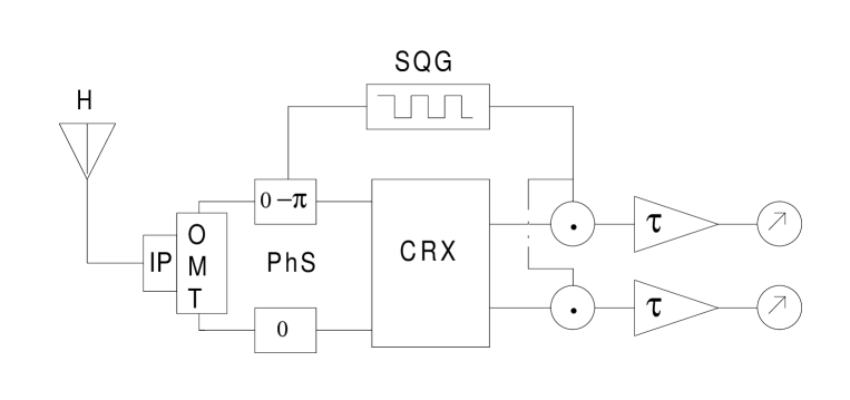
Figure 3: Modulated Correlation Polarimeter - H = Horn, IP = Iris Polarizer, OMT = Orthomode transducer, PhS = Phase shifter, CRX = Correlator, SQG = Square Wave Generator, . synchronous detector, $\tau$ = time integrator

3.2 Modulation and Offset Elimination

Phase modulation of the electric wave $E(t)$ is achieved including into arm 1 of the correlation receiver a ($0-\pi$), just after the OMT, a phase shifter, driven by a square wave signal of period $T_{mod}=1/\nu_{mod}$ (short compared to $\tau$),

$$r(t)=\left\{\begin{array}[]{cc}+1&~{}~{}~{}nT_{mod}<t<(n+\frac{1}{2})T_{mod}\\ -1&~{}~{}~{}~{}~{}~{}~{}(n+\frac{1}{2})T_{mod}<t<(n+1)T_{mod}\end{array}\right.$$ (14)

It multiplies $E_{1}$ by $\pm 1$. An identical phase shifter in channel 2, locked in a stable position, equalizes the attenuations in channel 1 and channel 2.

If $E_{1}(t)=E_{o1}(t)e^{i\omega t}$ and $E_{2}(t)=E_{o2}(t)e^{i(\omega t+\phi)}$, are the signals available at the OMT outputs, the inputs of the Phase Discriminator are

$$\left[\matrix{A\cr B\cr}\right]=\left[\matrix{k_{1}E_{1}(t)r(t)\cr k_{2}E_{2}(t)\cr}\right]=\left[\matrix{k_{1}E_{o1}e^{i\omega t}~{}r(t)\cr k_{2}E_{02}e^{i(\omega t+\phi+\theta)}\cr}\right]$$ (15)

where $k_{1}$ and $k_{2}$ account for the system gain between OMT and PD, and

$$\left[\matrix{S_{1}\cr S_{2}\cr}\right]=\left[\matrix{\delta_{1}[|k_{1}E_{1}|^{2}+|k_{2}E_{2}|^{2}]+\eta_{1}k_{1}k_{2}[E_{1}E_{2}\cos(\theta+\phi)]r(t)\cr\delta_{2}[|k_{1}E_{1}|^{2}+|k_{2}E_{2}|^{2}]+\eta_{2}k_{1}k_{2}[E_{1}E_{2}\sin(\theta+\phi)]r(t)\cr}\right]$$ (16)

are the outputs of the differential amplifiers.

The Phase Sensitive Detector multiplies $S_{1}$ and $S_{2}$ by $r^{\prime}(t)$, a function similar to $r(t)$, and integrates the product for a time $\tau$, giving:

$$\left[\matrix{O_{1}\cr O_{2}\cr}\right]=\left[\matrix{<S_{1}\times r^{\prime}(t)>\cr<S_{2}\times r^{\prime}(t)>\cr}\right]~{}=~{}$$

$$~{}~{}~{}~{}~{}~{}~{}~{}~{}=~{}\left[\matrix{\delta_{1}[~{}|k_{1}E_{1}|^{2}+|k_{2}E_{2}|^{2}]<r^{\prime}(t)>\cr\delta_{2}[~{}|k_{1}E_{1}|^{2}+|k_{2}E_{2}|^{2}]<r^{\prime}(t)>\cr}\right]~{}+~{}$$

$$~{}~{}~{}~{}~{}~{}~{}~{}~{}~{}~{}~{}~{}~{}~{}~{}~{}~{}~{}~{}~{}+~{}\left[\matrix{\eta_{1}k_{1}k_{2}[E_{1}E_{2}\cos(\theta+\phi)]<r(t)\times r^{\prime}(t)>\cr\eta_{2}k_{1}k_{2}[E_{1}E_{2}\sin(\theta+\phi)]<r(t)\times r^{\prime}(t)>\cr}\right]$$ (17)

Because $<r(t)>=0$ and $<r^{\prime}(t)>=0$ now the offset terms vanish even when $\delta_{i}\neq 0~{}(h_{i}\neq h_{i+1})$.

Three configurations are possible:

i) system unlocked: $r(t)$ and $r^{\prime}(t)$ are generated   independently   therefore  $<r(t)\times r^{\prime}(t)>=0$

In this condition (marked by apex $ul$)

$$\left[\matrix{O_{1}^{ul}\cr O_{2}^{ul}\cr}\right]=\left[\matrix{0\cr 0\cr}\right]$$ (18)

always.

ii) system locked: PSD and modulator are driven, in phase, by the same function $r^{\prime}(t)\equiv r(t)$ (condition marked by apex $l$).

Now $<r(t)\times r^{\prime}(t)>=<r^{2}(t)>=$ 1 therefore

$$\left[\matrix{O_{1}^{l}\cr O_{2}^{l}\cr}\right]=\left[\matrix{\eta_{1}k_{1}k_{2}<E_{1}E_{2}\cos(\theta+\phi)>\cr\eta_{2}k_{1}k_{2}<E_{1}E_{2}\sin(\theta+\phi)>\cr}\right]$$ (19)

and one gets the Stokes Parameter (see equations.12 and 13)

iii) system locked with a phase difference (time delay $\Delta t$) between the application of $r(t)$ to the modulator and to the PSD ($r^{\prime}(t)=r(t+\Delta t)$, condition marked by apex $\Delta$):

$$\left[\matrix{O_{1}^{\Delta}\cr O_{2}^{\Delta}\cr}\right]=\left[\matrix{\eta_{1}k_{1}k_{2}<E_{1}E_{2}\cos(\theta+\phi)r(t)r(t+\Delta t)>\cr\eta_{2}k_{1}k_{2}<E_{1}E_{2}\sin(\theta+\phi)r(t)r(t+\Delta t)>\cr}\right]$$ (20)

Because $T_{mod}$ is small compared to $\tau$ and the time during which the amplitude $E_{01}$ and $E_{02}$ of $E_{1}$ and $E_{2}$ are expected to vary, we can write

$$\left[\matrix{O_{1}^{\Delta}\cr O_{2}^{\Delta}\cr}\right]\simeq\left[\matrix{\eta_{1}k_{1}k_{2}<E_{1}E_{2}\cos(\theta+\phi)><r(t)r(t+\Delta t)>\cr\eta_{2}k_{1}k_{2}<E_{1}E_{2}\sin(\theta+\phi)><r(t)r(t+\Delta t)>\cr}\right]~{}=~{}$$

$$~{}~{}~{}~{}~{}~{}~{}~{}~{}~{}=F~{}\left[\matrix{\eta_{1}k_{1}k_{2}<E_{1}E_{2}\cos(\theta+\phi)>\cr\eta_{2}k_{1}k_{2}<E_{1}E_{2}\sin(\theta+\phi)>\cr}\right]$$ (21)

where

$$F~{}=~{}<r(t)r(t+\Delta t)>~{}=~{}\frac{~{}1}{~{}T}\int_{0}^{T}{r(t)r(t+\Delta t)dt}~{}=~{}$$

$$~{}~{}~{}~{}~{}~{}~{}~{}=~{}~{}1~{}-~{}4~{}\frac{~{}|\Delta t|}{T}~{}~{}~{}~{}~{}~{}(-\frac{~{}T}{~{}2}\leq\Delta t\leq+\frac{~{}T}{~{}2}~{})$$ (22)

When $\Delta t\neq 0$ and $\Delta t\neq\pm T/2$,  $~{}|F|<1$ and a reduction of the system sensitivity occurs.

3.3 Synchronous Detection and Noise reduction

So far we neglected the system noise. Let‘s now call ${\varepsilon}_{i}$ the noise produced in channel $i$ and $\psi_{ri}(t)$ a random phase. When we add it to the signal $E_{i}$ equations 15 and 17 become:

$$\left[\matrix{A\cr B\cr}\right]=\left[\matrix{k_{1}[E_{1}r(t)+{\varepsilon}_{1}e^{i\psi_{r1}(t)}]\cr k_{2}[E_{2}e^{i(\phi+\theta)}+{\varepsilon}_{2}e^{i\psi_{r2}(t)}]\cr}\right]$$ (23)

and

$$\left[\matrix{O_{1}\cr O_{2}\cr}\right]~{}=~{}\left[\matrix{\delta_{1}[~{}|k_{1}E_{1}|^{2}+|k_{2}E_{2}|^{2}+|k_{1}\varepsilon_{1}|^{2}+|k_{2}\varepsilon_{2}|^{2})]<r^{\prime}(t)>\cr\delta_{2}[~{}|k_{1}E_{1}|^{2}+|k_{2}E_{2}|^{2}+|k_{1}\varepsilon_{1}|^{2}+|k_{2}\varepsilon_{2}|^{2})]<r^{\prime}(t)>\cr}\right]~{}+~{}$$

$$~{}~{}~{}~{}~{}~{}~{}~{}~{}~{}~{}~{}~{}+~{}\left[\matrix{\eta_{1}k_{1}k_{2}[E_{1}E_{2}\cos(\theta+\phi)]<r(t)\times r^{\prime}(t)>\cr\eta_{2}k_{1}k_{2}[E_{1}E_{2}\sin(\theta+\phi)]<r(t)\times r^{\prime}(t)>\cr}\right]$$

$$~{}~{}~{}~{}~{}~{}~{}~{}~{}~{}~{}~{}~{}~{}~{}~{}~{}~{}~{}~{}~{}~{}~{}~{}~{}~{}+~{}\left[\matrix{<{\it N}_{1}\times r^{\prime}+{\it N}^{*}_{1}>\cr<{\it N}_{2}\times r^{\prime}+{\it N}^{*}_{2}>\cr}\right]$$ (24)

where

$$\left[\matrix{{\it N}_{1}\cr{\it N}_{2}\cr}\right]=2~{}\left[\matrix{\delta_{1}\cr\delta_{2}\cr}\right]~{}k_{2}^{2}{\varepsilon}_{2}E_{2}~{}+~{}\left[\matrix{\eta_{1}\cr\eta_{2}\cr}\right]~{}k_{1}k_{2}\varepsilon_{1}(E_{2}~{}+~{}{\varepsilon}_{2})$$ (25)

and

$$\left[\matrix{{\it N}_{1}^{*}\cr{\it N}_{2}^{*}\cr}\right]=2~{}\left[\matrix{\delta_{1}\cr\delta_{2}\cr}\right]~{}k_{1}^{2}\varepsilon_{1}E_{1}~{}+~{}\left[\matrix{\eta_{1}\cr\eta_{2}\cr}\right]k_{1}k_{2}~{}\varepsilon_{2}~{}E_{1}$$ (26)

are noise terms (${\varepsilon}_{1}$ and ${\varepsilon}_{2}$ have random phases). As in equation 17 the offset terms, (which now include $\varepsilon_{1}^{2}$ and $\varepsilon_{2}^{2}$) vanish.

To appraise the filter action of the synchronous detector we have to evaluate the noise variance going back to the time domain, (see equations 2, 3 and 4). By integration of equations 24, 25 and 26 over the frequency bandwith of the receiver we get the total power measured at the system output:

$$\left[\matrix{<V_{1}(t)>\cr<V_{2}(t)>\cr}\right]~{}=~{}\left[\matrix{<S_{1}(t)+V_{n,1}(t)\times r(t)+V_{n,1}^{*}>\cr<S_{2}(t)+V_{n,2}(t)\times r(t)+V_{n,2}^{*}>\cr}\right]$$ (27)

where $S_{i}(t)$ is the power of the signal, $V_{n,i}(t)$ and $V_{n,i}^{*}(t)$ are the power of the noise associated to $N_{i}$ and $N_{i}^{*}$ respectively.

We then compute the ratio between the standard deviations of the noise calculated when the system is locked and unlocked:

$$R~{}=~{}\frac{\sigma_{l}}{\sigma_{ul}}~{}=~{}\sqrt{\frac{\sigma^{2}_{V_{n,i}\times r}~{}+~{}\sigma^{2}_{V^{*}_{n,i}}}{\sigma^{2}_{V_{n,i}}~{}+~{}\sigma^{2}_{V^{*}_{n,i}}}}$$ (28)

Assuming the worst conditions ($1/f$ noise dominant everywhere) for the power spectra of $V_{n,i}$ and $V_{n,i}^{*}$ we set $w_{V_{n,i}}=A_{i}/\nu$ and $w_{V_{n,i}^{*}}=A_{i}^{*}/\nu$. Moreover $k_{1}\simeq k_{2}$,  ${\varepsilon}_{1}\simeq{\varepsilon}_{2}\simeq{\varepsilon}$,  $E_{1}\simeq E_{2}\simeq E$,  $N_{1}\simeq N_{2}\simeq N$,  $N_{1}^{*}\simeq N_{2}^{*}\simeq N^{*}$,  $A_{1}\simeq A_{2}\simeq A$,  $A_{1}^{*}\simeq A_{2}^{*}\simeq A^{*}$,  $V_{n,1}\simeq V_{n,2}\simeq V_{n}$,  $V_{n,1}^{*}\simeq V_{n,2}^{*}\simeq V_{n}^{*}$ and $\delta_{1}\simeq\delta_{2}\simeq\delta<<\eta\simeq\eta_{1}\simeq\eta_{2}$. It follows  $({\it N}^{*}/{{\it N}})~{}\simeq~{}{E}/(E+\varepsilon)<1$ and, when $E$ is small compared to the system noise, (as usual when we look for the fine structures of the CMB), $N^{*}<<N$,  $A>>A^{*}$ and $\sigma^{2}_{V_{n}}=A\ln{(T/\tau)}>>\sigma^{2}_{V_{n}^{*}}=A^{*}\ln{(T/\tau)}$.

To get $\sigma_{V_{n,i}\times r}$ first of all we compute the power spectrum $w_{V_{n,i}\times r}(\nu)$ of $V_{n,i}\times r$. Calculations (see Appendix A and [Spiga 2000]) give (here an in the following we omit all $i$ indexes)

$$w_{V_{n}\times r}(\nu)=\frac{4}{\pi^{2}}\sum_{0}^{\infty}\frac{1}{(2k+1)^{2}}\frac{A}{|\nu-\nu_{k}|}+\frac{4}{\pi^{2}}\sum_{0}^{\infty}\frac{1}{(2k+1)^{2}}\frac{A}{|\nu+\nu_{k}|}$$ (29)

Because $<V_{n}\times r>=0$ from  equation 4 follows:

$$\sigma_{V_{n}\times r}^{2}=\int_{\nu_{min}}^{\nu_{max}}w_{V_{n}\times r}(\nu)\,d\nu=\int_{1/T}^{1/\tau}w_{V_{n}\times r}(\nu)\,d\nu=$$

$$=\frac{4}{\pi^{2}}\sum_{0}^{\infty}\frac{A}{(2k+1)^{2}}\int_{1/T}^{1/\tau}\frac{1}{\nu_{k}-\nu}\,d\nu+\frac{4}{\pi^{2}}\sum_{0}^{\infty}\frac{A}{(2k+1)^{2}}\int_{1/T}^{1/\tau}\frac{1}{\nu_{k}+\nu}\,d\nu$$

$$=\frac{4A_{i}}{\pi^{2}}\sum_{0}^{\infty}\frac{1}{(2k+1)^{2}}\left[\ln\left(\frac{\nu_{k}-1/T}{\nu_{k}-1/\tau}\right)+\ln\left(\frac{\nu_{k}+1/\tau}{\nu_{k}+1/T}\right)\right]$$ (30)

($1/T\ll 1/\tau\ll\nu_{k}$ for each $k$).

Finally neglecting $k>O^{3}$ terms, we get

$$R~{}=~{}\frac{\sigma_{l}}{\sigma_{ul}}=\sqrt{\frac{\ln\left(\frac{\displaystyle\nu_{mod}-1/T}{\displaystyle\nu_{mod}-1/\tau}\right)+\ln\left(\frac{\displaystyle\nu_{mod}+1/\tau}{\displaystyle\nu_{mod}+1/T}\right)}{2\ln\frac{\displaystyle T}{\displaystyle\tau}}}~{}\simeq$$

$$~{}~{}~{}~{}~{}~{}~{}~{}~{}~{}~{}~{}~{}~{}~{}~{}~{}~{}~{}~{}~{}~{}~{}\simeq~{}\sqrt{\frac{(\nu_{max}~{}-~{}\nu_{min})/\nu_{mod}}{\ln(\nu_{max}/\nu_{min})}}$$ (31)

Discussion

Above we got formulae which can be used to evaluate the noise reduction $R$ or, equivalently, the improvement of the system sensitivity $1/R$ one obtains adding phase modulation and synchronous detection to a correlation receiver. Assuming for instance $\nu_{mod}=1kHz$, $\tau=5\>sec~{}(\nu_{max}=0.2Hz)$ and $T=60\>min~{}(\nu_{min}=2.8~{}10^{-4}Hz)$, as common in CMB observations, we get $R\simeq 5.5~{}10^{-3}$ and $1/R\simeq 180$. In practice the effective reduction can be smaller. In fact:

i)We assumed square wave modulation. It gives maximum efficiency, because the modulator reaches almost immediately a well defined status, and keep it for almost $50\%$ of the modulation cycle. However the circuits which carries out this operation must be carefully studied because spurious signals are easily triggered by sharp transitions. For that reason sine wave modulation is sometimes preferred. It gives smooth transitions therefore the generation of spurious signals can be more easily controlled. However the signal which drives the modulator varies sinusoidally therefore the modulator response can vary and during an important fraction the modulation cycle be poorly defined.

ii)No matter which shape is preferred, practical modulating functions, modulators and detectors are only approximations of the mathematical functions we assumed. Deviations of the real components from their model as well as phase dependence of the attenuation and impedance of the modulator and detector may produce spurious modulations and/or cycle asymmetries. Because when present, they give rise to $<r>\neq 0$ and/or $<V\times r>\neq 0$ these effects must be carefully removed once again through proper design of circuits and devices. Residuals which should survive can be cancelled by fine shaping the function which drives the synchronous detector (e.g. [Sironi et al. 1990])

iii)For technical reasons sometimes the modulator - demodulator loop does not include the system front end. For instance in the most recent model (Mk-3) of the Milano Polarimeter the front end has been set outside the loop because no reliable cryogenic phase shifter was available ([Sironi et al. 2001]). In this case to analyze the system we have to split gain and noise in channel 1 in two components: $k_{01}$ and $\varepsilon_{01}$, gain and noise of the section which precedes the loop, $k_{11}$ and $\varepsilon_{11}$, gain and noise of the section inside the loop. Now  $k_{1}=k_{01}k_{11}$, $\varepsilon_{1}=\varepsilon_{01}+(k_{11}/k_{1})\varepsilon_{11}~{}=~{}(\alpha+\beta)\varepsilon_{1}$   ($\alpha=\varepsilon_{01}/\varepsilon_{1}$,   $\beta=(k_{11}/k_{1})\varepsilon_{11}/\varepsilon_{1}$),    and equation 23 becomes

$$\left[\matrix{A\cr B\cr}\right]=\left[\matrix{k_{1}[(E_{1}+\varepsilon_{01}e^{i\psi_{r01}})r(t)+k_{11}{\varepsilon}_{11}e^{i\psi_{r1}(t)}]\cr k_{2}[E_{2}e^{i(\phi+\delta)}+{\varepsilon}_{2}e^{i\psi_{r2}(t)}]\cr}\right]$$ (32)

By an analysis similar to the one we made before, for the noise terms we get now:

$$\left[\matrix{{\it N^{\prime}}_{1}\cr{\it N^{\prime}}_{2}\cr}\right]=2~{}\left[\matrix{\delta_{1}\cr\delta_{2}\cr}\right]~{}[k_{1}^{2}{\varepsilon}_{01}E_{1}~{}+~{}k_{2}^{2}{\varepsilon}_{2}E_{2}]~{}+~{}\left[\matrix{\eta_{1}\cr\eta_{2}\cr}\right]~{}k_{11}k_{2}\varepsilon_{11}(E_{2}~{}+~{}{\varepsilon}_{2})$$

$$~{}~{}~{}~{}~{}~{}~{}~{}~{}~{}~{}~{}~{}~{}~{}~{}~{}~{}~{}\simeq~{}\beta~{}\left[\matrix{{\it N}_{1}\cr{\it N}_{2}\cr}\right]~{}<~{}\left[\matrix{{\it N}_{1}\cr{\it N}_{2}\cr}\right]$$ (33)

and

$$\left[\matrix{{\it N^{\prime}}_{1}^{*}\cr{\it N^{\prime}}_{2}^{*}\cr}\right]=2~{}\left[\matrix{\delta_{1}\cr\delta_{2}\cr}\right]~{}k_{1}k_{11}\varepsilon_{11}(E_{1}~{}+~{}{\varepsilon}_{01})~{}+$$

$$~{}~{}~{}~{}~{}~{}~{}~{}~{}~{}+~{}\left[\matrix{\eta_{1}\cr\eta_{2}\cr}\right]~{}k_{1}k_{2}[E_{1}\varepsilon_{2}~{}+~{}{\varepsilon}_{01}(E_{2}~{}+~{}\varepsilon_{2})]$$

$$~{}~{}~{}~{}~{}~{}~{}~{}~{}~{}~{}~{}~{}~{}~{}~{}~{}~{}\simeq~{}\left[\matrix{{\it N}_{1}^{*}\cr{\it N}_{2}^{*}\cr}\right]~{}(1~{}+~{}\alpha(1~{}+~{}\varepsilon/E)~{}>~{}\left[\matrix{{\it N}_{1}^{*}\cr{\it N}_{2}^{*}\cr})\right]$$ (34)

where, to evaluate the approximated expression, we set $\varepsilon_{1}\simeq\varepsilon_{2}\simeq\varepsilon$ and $E_{1}\simeq E_{2}\simeq E$. The noise component ${\it N^{\prime}}^{*}$ unaffected by modulation/demodulation, is now larger by a factor $\simeq 1~{}+~{}(\varepsilon_{01}/\varepsilon_{1})~{}+~{}(\varepsilon_{01}/E_{1})$.   To keep it small and preserve the efficiency of the modulation/demodulation process, $\varepsilon_{01}$ and $k_{01}$ must be small compared to $\varepsilon_{1}$ and $k_{1}$ and, even more important, possibly free from $1/f$ contribution. Viceversa the component of the total noise one can control through modulation, $\it{N^{\prime}}$, decreases by $\beta$.

iv)Last but not least $\nu_{mod}$ must be far from harmonics of all periodic signal signals used into the receiver. Among them the frequency $\nu_{ac}$ of the AC power supply is particularly dangerous: it can in fact induce, through residuals ripples on the DC outputs of the power supply which feed amplifiers and active components, modulated signals which are picked up by the synchronous detector if $\nu_{mod}$ is close to harmonics of $\nu_{ac}$.

All the effects we listed above reduce the efficiency of the modulation / synchronous detection techniques in improving the stability and in rejecting the noise of a radiometer. By carefull design of the circuitry which realizes the system the degradation of R can however be contained sufficiently to make it a second order effect.

The above results have been obtained assuming a phase modulated correlation receiver. They can be extended to other radiometer configurations, like the classical Dicke Receiver ([Kraus 1966]) or bolometric systems which use amplitude modulation. In doing it we must remember that modulation and synchronous detection have different effects on the performance of a receiver. An important effect of modulation is a shift of the average output of the receiver. This shift can be used to bring to zero the average value of the receiver output, making the system insensitive to gain fluctuations and allowing large amplifications without saturation. Synchronous detection improve the signal to noise ratio, creating a filter which excludes signals not marked by modulation and cutting the components of the noise at frequency different from and below $\nu_{mod}$.

Used in the past for classical radioastronomical observations and in many physical experiments (the so called lock in technique) modulation and synchronous detection are today essential to reach the sensitivities necessary to study the fine structures of the CMB.

Appendix A Appendix A : Power spectrum of the modulated noise $(V\times r)$

By proper choice of $t$, the square wave $r(t)$ of period $T_{mod}=1/\nu_{mod}$ can be represented by a Fourier serie containing only $\cos$ terms and $\nu_{mod}$ odd multiples $\nu_{k}=(2k+1)\nu_{mod}$:

$$r(t)=\frac{4}{\pi}\sum_{k=0}^{+\infty}\frac{(-1)^{k}}{2k+1}\cos(2\pi\nu_{k}t)$$ (35)

The noise $V$ can be written as a Fourier integral

$$V(t)=\int_{-\infty}^{+\infty}a(\nu)e^{i(2\pi\nu t+\psi_{\nu}(t))}\,d\nu$$ (36)

where $\psi_{\nu}(t)$ is a randomly variable phase (here and in the following we will omit pedix $i$ which marks the system channel). Therefore

$$V(t)\times r(t)=\int_{-\infty}^{+\infty}a(\nu)\cos(2\pi\nu t+\psi_{\nu}(t))\ d\nu\times\ \frac{4}{\pi}\sum_{0}^{\infty}\frac{(-1)^{k}}{2k+1}\cos(2\pi\nu_{k}t)$$

$$+i\int_{-\infty}^{+\infty}a(\nu)\sin(2\pi\nu t+\psi_{\nu}(t))\ d\nu\times\ \frac{4}{\pi}\sum_{0}^{\infty}\frac{(-1)^{k}}{2k+1}\cos(2\pi\nu_{k}t)$$ (37)

Using standard trigonometric formulae we can write

$$V(t)\times r(t)=\frac{2}{\pi}\sum_{k=0}^{+\infty}\frac{(-1)^{k}}{2k+1}\times$$

$$\times\bigl{\{}\int_{-\infty}^{+\infty}a(\nu)[\cos(2\pi(\nu+\nu_{k})t+\psi_{\nu}(t))+\cos(2\pi(\nu-\nu_{k})t+\psi_{\nu}(t))]\ d\nu+$$

$$+i\int_{-\infty}^{+\infty}a(\nu)[\sin(2\pi(\nu+\nu_{k})t+\psi_{\nu}(t))+\sin(2\pi(\nu-\nu_{k})t)+\psi_{\nu}(t)]\ d\nu\bigl{\}}$$ (38)

Rearranging terms and omitting for semplicity the time dependence of $\psi$ we get:

$$\int_{-\infty}^{+\infty}a(\nu)[\cos(2\pi(\nu+\nu_{k})t+\psi_{\nu})+\cos(2\pi(\nu-\nu_{k})t+\psi_{\nu})]d\nu\ =$$

$$=\int_{0}^{+\infty}a(\nu)\cos(2\pi(\nu+\nu_{k})t+\psi_{\nu})d\nu+\int_{0}^{+\infty}a(\nu)\cos(2\pi(\nu-\nu_{k})t+\psi_{\nu})d\nu+$$

$$+\int_{-\infty}^{0}a(\nu)\cos(2\pi(\nu+\nu_{k})t+\psi_{\nu})d\nu+\int_{-\infty}^{0}a(\nu)\cos(2\pi(\nu-\nu_{k})t+\psi_{\nu})d\nu=$$

$$=\int_{+\nu_{k}}^{+\infty}a(\nu-\nu_{k})\cos(2\pi\nu t+\psi_{\nu-\nu_{k}})d\nu+\int_{-\infty}^{+\nu_{k}}a(\nu-\nu_{k})\cos(2\pi\nu t+\psi_{\nu-\nu_{k}})d\nu+$$

$$+\int_{-\nu_{k}}^{+\infty}a(\nu+\nu_{k})\cos(2\pi\nu t+\psi_{\nu+\nu_{k}})d\nu$$

$$~{}~{}~{}~{}~{}~{}~{}~{}~{}~{}~{}~{}+\int_{-\infty}^{-\nu_{k}}a(\nu+\nu_{k})\cos(2\pi\nu t+\psi_{\nu+\nu_{k}})d\nu$$ (39)

and

$$~{}~{}~{}~{}~{}\int_{-\infty}^{+\infty}a(\nu)[\sin(2\pi(\nu+\nu_{k})t+\psi_{\nu})+\sin(2\pi(\nu-\nu_{k})t+\psi_{\nu})]d\nu\ =$$

$$=\int_{+\nu_{k}}^{+\infty}a(\nu-\nu_{k})\sin(2\pi\nu t+\psi_{\nu-\nu_{k}})d\nu+\int_{-\infty}^{+\nu_{k}}a(\nu-\nu_{k})\sin(2\pi\nu t+\psi_{\nu-\nu_{k}})d\nu+$$

$$+\int_{-\nu_{k}}^{+\infty}a(\nu+\nu_{k})\sin(2\pi\nu t+\psi_{\nu+\nu_{k}})d\nu$$

$$+\int_{-\infty}^{-\nu_{k}}a(\nu+\nu_{k})\sin(2\pi\nu t+\psi_{\nu+\nu_{k}})d\nu$$ (40)

Therefore

$$V(t)\times\ r(t)=\frac{2}{\pi}\sum_{k=0}^{+\infty}\frac{(-1)^{k}}{2k+1}\left[\int_{+\nu_{k}}^{+\infty}a(\nu-\nu_{k})\exp[i(2\pi\nu t+\psi_{\nu-\nu_{k}})]d\nu\right.+$$

$$+\int_{-\infty}^{+\nu_{k}}a(\nu-\nu_{k})\exp[i(2\pi\nu t+\psi_{\nu-\nu_{k}})]d\nu$$

$$+\int_{-\nu_{k}}^{+\infty}a(\nu+\nu_{k})\exp[i(2\pi\nu t+\psi_{\nu+\nu_{k}})]d\nu+$$

$$+\left.\int_{-\infty}^{-\nu_{k}}a(\nu+\nu_{k})\exp[i(2\pi\nu t+\psi_{\nu+\nu_{k}})]d\nu\right]$$ (41)

Because $\psi_{\nu\pm\nu_{k}}$ is a random function of $\nu$, the $k$ component of the power spectrum of $V\times r$ is a sum of power spectra:

$$w_{k}(\nu)~{}=~{}\frac{4}{\pi^{2}(2k+1)^{2}}\left\{\begin{array}[]{cc}|a(-\nu-\nu_{k})|^{2}&~{}~{}~{}~{}~{}-\infty<\nu<-\nu_{k}\\ |a(+\nu+\nu_{k})|^{2}&~{}~{}~{}~{}~{}-\nu_{k}<\nu<+\infty\end{array}\right.~{}~{}+$$

$$~{}~{}~{}~{}~{}~{}~{}~{}~{}~{}~{}~{}~{}~{}~{}+\left\{\begin{array}[]{cc}|a(\nu_{k}-\nu)|^{2}&~{}~{}~{}~{}~{}-\infty<\nu<+\nu_{k}\\ |a(\nu-\nu_{k})|^{2}&~{}~{}~{}~{}~{}+\nu_{k}<\nu<+\infty\end{array}\right.$$ (42)

which, when the noise is $1/f$ noise ($|a(\nu)|^{2}=|a(-\nu)|^{2}=A/|\nu|)$ becomes

$$w_{k}(\nu)=\frac{4}{\pi^{2}(2k+1)^{2}}\left[\frac{A}{|\nu-\nu_{k}|}+\frac{A}{|\nu+\nu_{k}|}\right]$$ (43)

Because the phases of the $w_{k}$ terms vary very rapidly in a random way (they are calculated at frequencies different for each $k$), the total power spectrum is obtained adding the incoherent terms $w_{k}$

$$w_{V\times r}(\nu)=\frac{4}{\pi^{2}}\sum_{0}^{\infty}\frac{1}{(2k+1)^{2}}\frac{A}{|\nu-\nu_{k}|}+\frac{4}{\pi^{2}}\sum_{0}^{\infty}\frac{1}{(2k+1)^{2}}\frac{A}{|\nu+\nu_{k}|}$$ (44)

References

- [De Bernardis 2000] De Bernardis, P. et al. 2000, Nature, 404, 955
- [Hanany 2000] Hanay, S. et al. 2000, ApJ, 545, L5
- [Hedman et al. 2001] Hedman, M.M. et al. 2001, ApJ, 548, L111
- [Keating et al. 2001] Keating, B.G. et al. 2001, ApJ, 560, L1
- [Kraus 1966] Kraus, J.D.: Radioastronomy, McGraw-Hill, New York 1966
- [MAP 2001] http:map.gsfc.nasa.gov and references therein
- [Partridge 1995] Partridge, R.B.: 3K:The Cosmic Microwave Background Radiation Cambridge University Press, Cambridge (UK), 1995
- [Peverini et al. 2001] Peverini, O. A. et al. 2002, Workshop on Astrophysical Polarized Backgrounds Bologna 2002, AIP Conf. Proc. : in press
- [Rohlfs 86] Rohlfs, K.: Tools of Radioastronomy, Springer Verlag , Berlin 1986
- [Sironi et al. 1990] Sironi, G. et al. 1990: Meas. Sci. Technol. 1, 1119
- [Sironi et al. 1997] Sironi, G. et al. 1997, PASP 141, 116
- [Sironi et al. 1998] Sironi, G. et al. 1998, NewA, 3, 1
- [Sironi 2000] Sironi, G. 2000, NewA Rev., 43, 243
- [Sironi et al. 2001] Sironi, G. 2001: PASA Proc. : in press
- [Smoot 1992] Smoot, G.F. et al. 1992, ApJ, 396, L1
- [Spiga 2000] Spiga, D. 2000: Thesis for a Physics Degree, University of Milano
- [SPOrt 2001] Caretti, E. et al. 2001: in Astrophysical Polarized Backgrounds - Bologna 2001, AIP Conf. Proc.: in press, and http:sport.tesre.bo.cnr.it/ and references therein
- [Staggs et al. 1999] Staggs, S.T., Gundersen, J.O. and Church, S.E. 1999: in Microwave Foregrounds, A de Oliveira-Costa and M. Tegmark eds., ASP, S.Francisco 1999
- [Staggs et al. 2001] Staggs, S. and Church, S. 2001: Experimental CMB Status and Prospects: A report from Snowmass 2001, astro-ph/0111576v1
- [Torbet et al. 1999] Torbet E. et al. 1999, ApJ, 521, L79
- [Van der Ziel 1954] Van der Ziel, A. 1954 : Noise, Prentice Hall, New York 1954
- [Zannoni 2000] Zannoni, M. 2000: PhD Thesis, University of Milano