Transformation Properties of External Radiation Fields,
Energy-Loss Rates and Scattered Spectra,
and a Model for Blazar Variability

Abstract

We treat transformation properties of external radiation fields in the proper frame of a plasma moving with constant speed. The specific spectral energy densities of external isotropic and accretion-disk radiation fields are derived in the comoving frame of relativistic outflows, such as those thought to be found near black-hole jet and gamma-ray burst sources. Nonthermal electrons and positrons Compton-scatter this radiation field, and high-energy protons and ions interact with this field through photomeson and photopair production. We revisit the problem of the Compton-scattered spectrum associated with an external accretion-disk radiation field, and clarify a past treatment by the authors. Simple expressions for energy-loss rates and Thomson-scattered spectra are given for ambient soft photon fields consisting either of a surrounding external isotropic monochromatic radiation field, or of an azimuthally symmetric, geometrically thin accretion-disk radiation field. A model for blazar emission is presented that displays a characteristic spectral and variability behavior due to the presence of a direct accretion-disk component. The disk component and distinct flaring behavior can be bright enough to be detected from flat spectrum radio quasars with GLAST. Spectral states of blazars are characterized by the relative importance of the accretion-disk and scattered radiation fields and, in the extended jet, by the accretion disk, inner jet, and cosmic microwave background radiation fields.

1 Introduction

The discovery of intense medium-energy gamma radiation from over 60 blazar AGNs with the EGRET instrument on the Compton Observatory (Hartman et al., 1999) shows that nonthermal gamma-ray production is an important dissipation mechanism of jet energy generated by black-hole accretion. In the standard model for blazars, nonthermal synchrotron emission is radiated by electrons accelerated via first-order shock Fermi processes to Lorentz factors $\gamma\lower 2.15277pt\hbox{$\;\buildrel\ll\over{\sim}\;$}5\times 10^{7}/\sqrt{B({\rm G})}$, where $B$ is the comoving magnetic field. These electrons will Compton-scatter all available radiation fields, including the internal synchrotron field and the external radiation fields intercepted by the jet. The intensities of the external ambient radiation fields, transformed to the comoving jet frame, are generally required to model the production spectra of blazars. External photon fields include the cosmic microwave background radiation (CMBR) field (e.g., Burbidge et al. (1974); Tavecchio et al. (2000); Dermer and Schlickeiser (1993), hereafter DS93), the accretion-disk radiation field (Dermer et al. (1992), DS93), the accretion-disk radiation field scattered by surrounding gas and dust (Sikora et al., 1994; Dermer, Sturner, and Schlickeiser, 1997), infrared emissions from hot dust or a molecular torus (Protheroe and Biermann, 1997; Blazejowski et al., 2000; Arbeiter, Pohl, and Schlickeiser, 2002), reflected synchrotron radiation (Ghisellini and Madau, 1996; Böttcher and Dermer, 1998), broad-line region atomic line radiation (Koratkar et al., 1998), etc.

Gamma rays in leptonic models of broadband blazar emission originate from synchrotron self-Compton (SSC) (Maraschi, Ghisellini, & Celotti, 1992; Bloom & Marscher, 1996; Tavecchio et al., 1998) or external Compton (EC) (e.g., Melia and Königl (1989), DS93, Böttcher, Mause, and Schlickeiser (1997); see Böttcher (2001) and Sikora & Madejski (2001) for recent reviews) processes. In hadronic models, secondary photopairs and photomesons are produced when energetic protons and ions interact with ambient synchrotron photons (e.g., Mannheim and Biermann (1992); Mannheim (1993)) and photons of the external field (Bednarek and Protheroe, 1999; Atoyan & Dermer, 2001). The spectral energy distribution of a blazar will consist, in addition to nonthermal synchrotron and SSC emissions, of secondary radiations that are a consequence of processes involving external soft photon fields. These radiations include neutral secondaries from hadrons, and the radiations produced when external soft photon fields are scattered by directly accelerated lepton primaries and lepton secondaries formed in photopair, photohadronic, and electromagnetic cascade processes. The intensities of the various components depend on the properties of the external fields, the properties of the relativistic outflows, and the time-dependent spectral injection of ions and electrons into the outflow. Given these conditions, the evolving particle and photon distributions and emergent radiation spectra can be derived for a specific model.

A significant modeling effort has been devoted to blazar studies. Where the synchrotron and SSC components are the dominant radiation processes, as appears to be the case in some X-ray bright BL Lac objects such as Mrk 421 and Mrk 501, observations of correlated X-ray/TeV loop patterns found in graphs of spectral index versus intensity are explained through combined particle acceleration, injection, and radiative loss effects (e.g., Kirk, Rieger, and Mastichiadis, 1998; Li and Kusunose, 2000). The spectral energy distributions of BL Lac objects are successfully modelled with synchrotron and SSC components from broken power-law electron distributions with low energy cutoffs, as in Mrk 501 (Mastichiadis and Kirk, 1997; Pian et al., 1998). Models for the spectral energy distributions of flat spectrum quasars, including external Compton components, have been presented for different spectral states by Hartman et al. (2001), Mukherjee et al. (1999), and Böttcher (1999), and in papers cited in the first paragraph.

More recently, Sikora et al. (2001) have presented a model for blazar variability with time-dependent injection into a relativistically moving blob that contains nonthermal electrons which are subject to radiative and adiabatic losses. The scattered radiation from an external, quasi-isotropic radiation field is treated, and evolving spectral energy distributions and light curves are calculated. No direct accretion disk field is however treated, though the emission sites could be within 0.1-1 pc of the black hole, where such components can make a significant contribution (Dermer and Schlickeiser, 1994). We show that the addition of the accretion-disk components produce light curves and correlated multifrequency behaviors that are quite distinct from the behavior calculated by Sikora et al. (2001). These distinct patterns are bright enought to be well detected with the upcoming Gamma ray Large Area Space Telescope (GLAST) mission, thus constraining the location of the shocks in gamma-ray blazars and the dominant spectral components.

In this paper, we revisit the transformation properties of the external radiation field, and clarify a past treatment by the authors (DS93). Here we adopt a formulation in terms of intensity rather than, as in DS93, photon number. The intensity formulation seems to offer a simpler method for comparing multiwavelength data, though the photon number approach perhaps simplifies the formulation of the scattering, attenuation, and secondary production interactions.

The jet plasma is assumed to be located along the symmetry axis of a geometrically-thin accretion disk. The intensity of photons in the jet frame depends on whether the accretion disk is optically thick or thin at large disk radii $R\gg r$, where $r$ is the distance of the jet plasma from the black hole. The treatment of DS93 used an optically-thin formulation with a volume-energy generation rate appropriate to disk accretion in a steady flow. DS93 assigned a blackbody temperature for the mean energy of the disk radiation field at different annuli, whereas a wide variety of models are possible. The radiation fields originating from radii $R\gg r$, though spectrally distinct between the optically-thin and -thick cases, give minor effect on the Thomson energy losses and scattered photon spectra.

The energy density of disk photons that are scattered to $\gamma$-ray energies by the jet electrons is shown to be dominated by photon production at $R\approx r$ in the near-field (NF) regime, and by the total black-hole power approximated as a receding point source in the far-field (FF) regime. The accretion-disk photons scattered by gas and dust surrounding the black hole can dominate the near- and far-field disk fields at large gravitational radii ($r_{g}=1.5\times 10^{14}M_{9}$ cm), depending on the relative transition radii where the NF, FF, and scattered external radiation fields dominate (Appendix A).

The transformed energy spectrum of the thermal accretion disk in the comoving frame displays a low-energy steepening for photons which originate primarily from radii $R\gg r$. This is an important effect in photohadronic calculations of very high energy secondary production, and is also important in $\gamma$-$\gamma$ transparency calculations (Atoyan & Dermer, 2002). Other photon sources can make an additional contribution in this range. Because the bulk of the black-hole accretion power is generated at small disk radii, the use of an optically-thin or optically-thick formulation at $R\gg r$ has negligible effect on the total scattered power for power-law electron injection with injection index $>2$. This article presents basic equations to calculate transformed external radiation fields from geometrically-thin accretion disks in the limiting optically-thin and optically-thick regimes.

Expressions for Thomson-scattered spectra from nonthermal electrons with arbitrary energy and isotropic comoving pitch-angle distributions are derived for external isotropic and direct accretion-disk radiation fields. The electron equation-of-motion is solved in the regime where the total synchrotron and external Thomson losses from the disk and quasi-isotropic external radiation fields dominate SSC losses. The evolving electron distribution is obtained through a continuity equation treatment with radiative losses on stationary electron injection over a range of radii, but here neglecting adiabatic losses. This simplified blazar model shows a dramatic change of spectral behavior if nonthermal particle acceleration continuously operates within $\approx 10^{2}$-$10^{4}r_{g}$ from the black-hole engine. In the model studied here, a pivoting of spectral shape is expected at a few GeV on time scales of days, with $\gamma$-ray spectral activity correlating with monotonic increases at IR and X-ray energies. Delayed radio activity is predicted as the emergent energized plasma blob expands and becomes optically thin to synchrotron self-absorption on the parsec scale, though this behavior is not modeled here. Campaigns employing GLAST accompanied by broadband monitoring at other frequencies can record multifrequency spectral flaring data and test the model.

Preliminaries of radiation theory and invariants are given in Sections 2 and 3, respectively. Section 4 treats the transformation of external radiation fields, specializing to the azimuthally symmetric and extreme-relativistic ($\Gamma\gg 1$) cases. The comoving specific spectral energy density for an optically-thick Shakura and Sunyaev (1973) accretion disk is derived in Section 5. Accretion-disk modeling is briefly mentioned (§5.1) before proceeding to derive the comoving energy spectrum of the disk field (§5.2). The same problem for an optically-thin disk is treated in Section 6, and comparison with the approach of DS93 is made in Section 7. The properties of the specific spectral energy density of the accretion-disk radiation field, transformed to the comoving fluid frame of the jet, are examined in Section 8.

Section 9 presents analytic forms for the energy-loss rates and spectra from various radiation processes, including synchrotron emission (§9.1), radiation from Thomson-scattered external isotropic monochromatic (§9.2) and accretion-disk fields in the near-field (§9.3) and far-field (§9.4) limits, and SSC radiation (§9.5). A simple model for blazar variability is presented in Section 10 in the limit that synchrotron and Thomson-scattered external radiation fields dominate the electron-energy loss rates. Model results for stationary particle acceleration and injection taking place within $\sim 10^{2}$-$10^{4}r_{g}$ from the black hole reveal a characteristic spectral behavior that joint radio/submillimeter/IR/X-ray/$\gamma$-ray campaigns can test. Detectability of blazar flares with GLAST is treated in Section 11, where multiwavelength light curves of a model blazar flare are presented.

The Appendices provide more detail on the derivations of the results in Section 9. In particular, Appendices A.6 and A.7 show that different spectral states of blazars and extended jets are defined by the simple relations in equations (A13) and (A15) which govern the relative imporatance of the accretion-disk, scattered, and CMBR fields. An important deficiency in the model is the treatment of Klein-Nishina effects in Compton scattering, which has been considered in the context of blazar physics by Böttcher, Mause, and Schlickeiser (1997), Georganopoulos, Kirk, & Mastichiadis (2001) and Dermer and Atoyan (2002). An analytic approach to this physics is given in Appendix D, including comparison with the paper by Georganopoulos, Kirk, & Mastichiadis (2001).

2 Preliminaries

We consider external radiation fields from optically-thick and optically-thin accretion disks, following preliminaries on radiation physics (Novikov and Thorne, 1973; Rybicki and Lightman, 1979). Our notation is such that a quantity $X_{\epsilon}$ has the full units of $X$, whereas differential quantities are denoted by $X(x_{1},x_{2};y)=\partial X(y)/\partial x_{1}\partial x_{2}$, where $y$ is a parameter.

The intensity

$$I_{\epsilon}(\Omega)={d{\cal E}\over dAdtd\epsilon d\Omega}$$ (1)

is defined such that $I_{\epsilon}(\Omega)dAdtd\Omega$ is the infinitesimal energy $d{\cal E}$ carried during infinitesimal time $dt$ by photons with dimensionless energy $\epsilon=h\nu/m_{e}c^{2}$ between $\epsilon$ and $\epsilon+d\epsilon$ that passes through area element $dA$ oriented normal to the direction of rays of light lying within the solid angle element $d\Omega$ about the direction $\vec{\Omega}$. Except for polarization, $I_{\epsilon}(\Omega;{\vec{x}},t)$ gives a complete description of the radiation field at location $\vec{x}$ and time $t$.

The quantity $dF_{\epsilon}=\mu I_{\epsilon}(\Omega)d\Omega$ is the differential spectral energy flux (units of ergs cm^-2 s^-1 $\epsilon^{-1}$) that passes through an area element oriented at an angle $\mu=\cos\theta=\hat{n}\cdot\vec{\Omega}$ to the rays within solid angle element $d\Omega$ about the direction $\vec{\Omega}$. The net flux $F_{\epsilon}(\hat{n})=\oint d\Omega\;\mu I_{\epsilon}(\Omega)$ depends on the orientation of the area element. Radiation fields that are azimuthally symmetric about some axis and that can be expanded in even powers of $\mu$ have zero net flux, that is, $F_{\epsilon}=0$. Obviously, the net flux of an isotropic radiation field is zero.

Because the momentum of a photon is $h\nu/c$, the component of momentum flux along $\hat{n}$ is given by $p_{\epsilon}$ (dynes cm${}^{-2}\epsilon^{-1}$) = $c^{-1}\oint d\Omega\;\mu^{2}I_{\epsilon}(\Omega)$. One factor of $\mu$ is from the projection of the area element, and the second is from the component of momentum along $\hat{n}$. Although $I_{\epsilon}(\Omega)\geq 0$ for all $\Omega$, $p_{\epsilon}$ can be $<0$ if the net momentum flux is directed opposite to $\hat{n}$. The total radiation pressure is $p=c^{-1}\int_{0}^{\infty}d\epsilon\oint d\Omega\;\mu^{2}I_{\epsilon}(\Omega)$.

The $\nu F_{\nu}$ energy flux (ergs cm^-2 s^-1) at frequency $\nu=m_{e}c^{2}\epsilon/h$ is $f_{\epsilon}(\hat{n})=\epsilon\,F_{\epsilon}=\epsilon\oint d\Omega\,\mu I_{\epsilon}(\Omega)$. The bolometric energy flux $\Phi(\hat{n})=\int_{0}^{\infty}d\epsilon\,\epsilon^{-1}f_{\epsilon}(\hat{n})=\int_{0}^{\infty}d\epsilon\oint d\Omega\,\mu I_{\epsilon}(\Omega)$. The specific spectral energy density $u(\epsilon,\Omega)=d{\cal E}/dVd\epsilon d\Omega$, and the spectral energy density $u(\epsilon)=\oint d\Omega\,u(\epsilon,\Omega)$. Note that $d{\cal E}=u(\epsilon,\Omega)dVd\epsilon d\Omega=u(\epsilon,\Omega)cdtdAd\epsilon d\Omega=I_{\epsilon}(\Omega)dAdtd\epsilon d\Omega$, so that

$$u(\epsilon,\Omega)=c^{-1}I_{\epsilon}(\Omega)\;.$$ (2)

The mean intensity $\bar{I}_{\epsilon}=({4\pi})^{-1}\oint d\Omega\;I_{\epsilon}(\Omega)=cu(\epsilon)/(4\pi)$. Thus $u(\epsilon)=4\pi\bar{I}_{\epsilon}/c$. The total radiation energy density $u=\int_{0}^{\infty}d\epsilon\;u(\epsilon)=4\pi c^{-1}\int_{0}^{\infty}d\epsilon\;\bar{I}_{\epsilon}$. The radiation pressure for an isotropic radiation field with (mean) intensity $\bar{I}_{\epsilon}^{iso}$ is $p=c^{-1}\int_{0}^{\infty}d\epsilon\oint d\Omega\;\mu^{2}\bar{I}_{\epsilon}^{iso}=(4\pi/3c)\int_{0}^{\infty}d\epsilon\;\bar{I}_{e}^{iso}$. Because $u=(4\pi/c)\int_{0}^{\infty}d\epsilon\;\bar{I}_{\epsilon}^{iso}$, we have

$$p=u/3\;$$ (3)

for an isotropic radiation field.

From conservation of energy, we can say that $d{\cal E}_{1}=I_{\epsilon,1}dA_{1}dtd\Omega_{1}d\epsilon_{1}=I_{\epsilon,2}dA_{2}dtd\Omega_{2}d\epsilon_{2}$ by following a bundle of rays from one area element to the next. The relationships between area elements separated by distance $d$, and the solid angles subtended by the bundle of rays at the two locations are $d\Omega_{1}=dA_{2}/d^{2}$ and $d\Omega_{2}=dA_{1}/d^{2}$. With $\epsilon_{1}=\epsilon_{2}=\epsilon$, $d\epsilon_{1}=d\epsilon_{2}=d\epsilon$, we obtain

$$I_{\epsilon,1}=I_{\epsilon,2}\;,\;\;{\rm or}\,\,dI_{\epsilon}/ds=0\;,\;$$ (4)

provided no absorption occurs as the light rays propagate. The equation of radiative transfer is

$${dI_{\epsilon}\over ds}=-\kappa_{\epsilon}I_{\epsilon}+j(\epsilon,\Omega)\;\;,\;\;{\rm or}\;\;\;{dI_{\epsilon}\over d\tau_{\epsilon}}=-I_{\epsilon}+S_{\epsilon},$$ (5)

where we define the photon-energy dependent spectral optical depth $\tau_{\epsilon}=\kappa_{\epsilon}ds$ in terms of the $\epsilon$-dependent spectral absorption coefficient $\kappa_{\epsilon}$ (cm^-1) and the emissivity $j(\epsilon,\Omega)=d{\cal E}/dVdtd\epsilon d\Omega$. The source function is

$$S_{\epsilon}={j(\epsilon,\Omega)\over\kappa_{\epsilon}}\;.$$ (6)

The energy flux from a uniform brightness sphere of radius $R$ is an instructive example. In this case, $I_{\epsilon}(\Omega)=B_{\epsilon}$, where $B_{\epsilon}$ is independent of $\Omega$ by definition. Further defining $\int_{0}^{\infty}d\epsilon\,B_{\epsilon}=B$, we find that the total energy flux at the telescope aperture located a distance $d$ from the source is $\Phi(\hat{n})=\int_{0}^{\infty}d\epsilon\oint d\Omega\;\mu B_{\epsilon}=2\pi B\int_{\sqrt{1-R^{2}/r^{2}}}^{1}\;\mu\;d\mu=\pi BR^{2}/r^{2}$. Thus the energy flux at the surface of a uniform brightness sphere is $\pi B$. The energy flux at the surface of a blackbody radiator is $\sigma_{\rm SB}T^{4}$, where the Stefan-Boltzmann constant $\sigma_{\rm SB}=5.67\times 10^{-5}$ ergs s^-1 cm^-2 degrees^-4.

3 Invariant Quantities

The elementary invariants are the invariant 4-volume $d^{3}\vec{x}dt=dVdt$, the quantity $d^{3}\vec{p}/E$, and the invariant phase volume $d{\cal V}=d^{3}\vec{x}d^{3}\vec{p}$. Here $E$ is photon or particle energy, $p$ is momentum, and $d^{3}\vec{p}=p^{2}dpd\Omega$. The invariance of $d^{3}\vec{x}dt$ and $d^{3}\vec{p}/E$ can be demonstrated by calculating the Jacobian for transformations consisting of rotations and boosts. The invariance of $d{\cal V}$ follows by noting that $dt/E$ is the ratio of parallel 4-vectors (Blumenthal and Gould 1970).

Because the number N of particles or photons is invariant,

$${dN\over d{\cal V}}={1\over p^{2}}\;{dN\over dVdpd\Omega}={1\over(m_{e}c)^{3}\,\epsilon^{2}}\;{dN\over dVd\epsilon d\Omega}={1\over m_{e}^{4}c^{5}\epsilon^{3}}\,{dE\over dVd\epsilon d\Omega}=\epsilon^{-3}\;{u(\epsilon,\Omega)\over m_{e}^{4}c^{5}}\;,$$ (7)

where the latter three expressions apply to photons ($E=mc^{2}\epsilon$). Hence, $\epsilon^{-3}u(\epsilon,\Omega)$ and $\epsilon^{-3}I_{\epsilon}(\Omega)$ are invariants.

The function

$$E\;{dN\over d^{3}\vec{x}dtd^{3}\vec{p}}={1\over(m_{e}c)^{3}\epsilon^{2}}\;{dE\over dVdtd\epsilon d\Omega}={1\over(m_{e}c)^{3}\epsilon^{2}}\;j(\epsilon,\Omega)\;\;$$ (8)

is invariant, where the last two expressions apply to photons, implying that $\epsilon^{-2}j(\epsilon,\Omega)$ is invariant. This and the invariance of $\epsilon^{-3}I_{\epsilon}(\Omega)$ show from equation (6) that $\epsilon\kappa_{\epsilon}$ is invariant.

4 Transformation of External Radiation Fields

The photon energy $\epsilon$ and angle $\theta=\cos^{-1}\mu$ in the stationary frame of the accretion disk are given in terms of the comoving photon energy $\epsilon^{\prime}$ and direction cosine $\mu^{\prime}$ through the relations $\epsilon=\Gamma\epsilon^{\prime}(1+\beta_{\Gamma}\mu^{\prime})$, $\mu=(\mu^{\prime}+\beta_{\Gamma})/(1+\beta_{\Gamma}\mu^{\prime})$, and $\phi=\phi^{\prime}$. From the invariance of $u(\epsilon,\Omega)/\epsilon^{3}$, we have

$$u^{\prime}(\epsilon^{\prime},\Omega^{\prime})={u(\epsilon,\Omega)\over\Gamma^{3}(1+\beta_{\Gamma}\mu^{\prime})^{3}}\;,$$ (9)

For simplicity, we assume azimuthal symmetry about the axis of the boost to the comoving jet frame, moving with bulk Lorentz factor $\Gamma$ with respect to the stationary black hole system. For an isotropic external photon field, $u(\epsilon,\mu)={1\over 2}u(\epsilon)$. Hence $u^{\prime}(\epsilon^{\prime},\mu^{\prime})=u(\epsilon)/[2\Gamma^{3}(1+\beta_{\Gamma}\mu^{\prime})^{3}]$ in this case.

For an external isotropic monochromatic radiation field, $u(\epsilon)=u_{ext}\delta(\epsilon-\bar{\epsilon})$. Thus the comoving energy density

$$u_{ext}^{\prime}=\int_{0}^{\infty}d\epsilon^{\prime}\int_{-1}^{1}d\mu^{\prime}u^{\prime}(\epsilon^{\prime},\mu^{\prime})={u_{ext}\over 2\Gamma^{4}}\,\int_{-1}^{1}d\mu^{\prime}\,(1+\beta_{\Gamma}\mu^{\prime})^{-4}=u_{ext}\Gamma^{2}(1+{\beta_{\Gamma}^{2}\over 3})\;$$ (10)

(Dermer and Schlickeiser, 1994). Following the integration over energy, one sees that the angle-dependent specific energy density $u^{\prime}(\mu^{\prime})=u_{ext}/[2\Gamma^{4}(1+\beta_{\Gamma}\mu^{\prime})^{4}]$. The four powers of the Doppler factor $\delta=\Gamma(1+\beta_{\Gamma}\mu^{\prime})=[\Gamma(1-\beta_{\Gamma}\mu)]^{-1}$ are due to two powers of $\delta$ from the solid angle transformation, one from the energy transformation, and one from increased density due to length contraction. For $\Gamma\gg 1$, the specific energy density ranges in value from $\sim 8\Gamma^{4}u_{ext}$ at $\mu^{\prime}=-1$ to $\sim u_{ext}/(32\Gamma^{4})$ at $\mu^{\prime}=1$. The function plummets in value when $\mu^{\prime}\gtrsim-\beta_{\Gamma}$. Multiplying $u^{\prime}(\mu^{\prime}=-\beta_{\Gamma})\cong\Gamma^{4}u_{ext}/2$ by the characteristic solid angle element $\delta\Omega^{\prime}\sim\pi\theta^{\prime 2}\sim\pi/\Gamma^{2}$ gives $u^{\prime}_{ext}\cong(\pi/2)\Gamma^{2}u_{ext}$, which approximately recovers equation (10) when $\Gamma\gg 1$. The function $u^{\prime}(\epsilon^{\prime},\mu^{\prime})\cong 4\Gamma^{2}u_{ext}\delta(\epsilon^{\prime}-4\Gamma\bar{\epsilon}/3)\delta(\mu^{\prime}+1)/3$ provides a useful approximation in the limit $\Gamma\gg 1$, noting that $u^{\prime}_{ext}/n^{\prime}_{ext}=(1+\beta_{\Gamma}^{2}/3)\Gamma\bar{\epsilon}m_{e}c^{2}$. For isotropic external photons, the hardest and most intense radiation is directed opposite to the direction of motion of the jet plasma in the comoving frame.

Now consider the transformation of an isotropic, azimuthally symmetric power-law radiation field described by the function

$$u(\epsilon,\mu)=k_{\alpha}u_{ext}\epsilon^{-\alpha}\;,\;{\rm for~{}}\epsilon_{\ell}<\epsilon<\epsilon_{u}\;.$$ (11)

The normalization $u_{ext}=\int_{0}^{\infty}d\epsilon\int_{-1}^{1}d\mu\,u(\epsilon,\mu)$ gives

$$k_{\alpha}=\cases{{(1-\alpha)\over 2(\epsilon_{u}^{1-\alpha}-\epsilon_{\ell}^{1-\alpha})}\;,&for general $\alpha$\cr\cr[2\ln(\epsilon_{u}/\epsilon_{\ell})]^{-1}\;,&for $\alpha=1$ .\cr}\;\;$$ (12)

Equations (9) and (11) imply

$$u^{\prime}(\epsilon^{\prime},\mu^{\prime})={k_{\alpha}u_{ext}\epsilon^{\prime-\alpha}\over\Gamma^{3}(1+\beta_{\Gamma}\mu^{\prime})^{3+\alpha}}\;,\;{\rm for~{}}\epsilon_{\ell}<\Gamma\epsilon^{\prime}(1+\beta_{\Gamma}\mu^{\prime})<\epsilon_{u}\;,$$ (13)

which is easily shown to be normalized to $u^{\prime}_{ext}$ given by equation (10).

5 Specific Spectral Energy Density

The specific spectral energy density $u(\epsilon,\Omega;\vec{x},t)=c^{-1}I(\epsilon,\Omega)$ from equation (2). The external field at arbitrary locations can be obtained from the constancy of specific intensity, equation (4), if intervening absorption is negligible. This is the starting point for the calculations of external radiation fields, from which transformed fields can be obtained through equation (9).

We specialize to the calculation of the external radiation field emitted by steady, azimuthally symmetric emitting regions, as might correspond to thin accretion disks around supermassive black holes. We furthermore consider a geometry where the emitting surface of the disk is located on the symmetry plane, and assume that the disk thickness $h(R)$ at radius $R$ is $\ll R$. Thus

$$\mu={r\over\sqrt{r^{2}+R^{2}}}=(1+R^{2}/r^{2})^{-1/2}\;,\;\;R=r(\mu^{-2}-1)^{1/2}\;.$$ (14)

In the cool, optically-thick blackbody solution of Shakura and Sunyaev (1973), the disk emission is approximated by a surface radiating at the blackbody temperature associated with the local energy dissipation rate per unit surface area, which is derived from considerations of viscous dissipation of the gravitational potential energy of the accreting material (Shapiro & Teukolsky, 1983). One finds that the integrated emission spectrum measured far from the black hole varies $\propto\epsilon^{1/3}$ up to a maximum photon energy associated with the innermost stable orbit of the accretion disk. The optically-thick solution is unstable in the inner region near a black hole due to secular density/cooling instabilities (Lightman and Eardley, 1974) in some regimes of the Eddington ratio

$$\ell_{\rm Edd}={\eta\dot{m}c^{2}\over L_{\rm Edd}}\;,$$ (15)

where $\eta$ is the efficiency to transform accreted matter to escaping radiant energy. The Eddington luminosity $L_{\rm Edd}=1.26\times 10^{47}M_{9}$ ergs s^-1, where the mass of the central supermassive black hole is $M=10^{9}M_{9}M_{\odot}$ and the black hole is accreting mass at the rate $\dot{m}$ (gm s^-1).

The intensity of a blackbody is

$$I^{bb}_{\epsilon}(\Theta)={2c(m_{e}c^{2})\over\lambda_{\rm C}^{3}}\;{\epsilon^{3}\over[\exp(\epsilon/\Theta)-1]}\rightarrow{2c(m_{e}c^{2})\over\lambda_{\rm C}^{3}}\;\cases{\Theta\epsilon^{2}\;,\;\epsilon\ll\Theta&Rayleigh-Jeans regime\cr\cr\epsilon^{3}\exp(-\epsilon/\Theta)\;,\;\epsilon\gg\Theta&Wien regime\cr}\;\;,$$ (16)

where $\Theta=k_{\rm B}T/m_{e}c^{2}$ and $\lambda_{\rm C}=h/m_{e}c=2.426\times 10^{-10}$ cm is the electron Compton wavelength. For steady flows where the energy is derived from the viscous dissipation of the gravitational potential energy of the accreting matter, the radiant surface-energy flux

$${dE\over dAdt}={3GM\dot{m}\over 8\pi R^{3}}\;\varphi(R)$$ (17)

(Shakura and Sunyaev, 1973), where

$$\varphi(R)=[1-\beta_{i}(R_{i}/R)^{1/2}]\;,$$ (18)

$\beta_{i}\cong 1$, and $R_{i}=6GM/c^{2}$ for a Schwarzschild metric. Integrating equation (17) over a two-sided disk gives $\eta=1/12$. Assuming that the disk is as an optically-thick blackbody radiator, the effective temperature of the disk can be determined by equating equation (17) with the surface energy flux $\sigma_{\rm SB}T^{4}(R)$.

5.1 Disk Models

To calculate the scattered jet radiation spectrum from the disk-jet system, it is essential to properly characterize the accretion-disk geometry and emissivity. Observations suggest that the radius separating a geometrically-thin outer accretion disk from an optically-thin hot inner cloud or disk increases with decreasing $\ell_{\rm Edd}$ in the range $\ell_{\rm Edd}\lesssim$0.1. (see Liang (1998) for a review of accretion disks around galactic black hole sources). Within an advection-dominated accretion disk (ADAF) scenario (e.g., Esin, McClintock, & Narayan (1997); Di Matteo et al. (2000); Quataert & Gruzinov (2000)), the radiant luminosity from an accreting system declines markedly when $\ell_{\rm Edd}\ll 0.1$ due to the advection of photons into the black hole and the convection of angular momentum and mass outward due to convective instabilities in the advection-dominated flows. Thus $\eta=\eta(\dot{m})$ in eq. (15), and the radiant luminosity follows a steeper dependence than $L_{rad}\lower 2.15277pt\hbox{$\;\buildrel\propto\over{\sim}\;$}\ell_{\rm Edd}$ when $\ell_{\rm Edd}\ll 0.1$. The radio-loud branch of accreting black holes seems to be found in the convectively unstable, low Eddington luminosity regime.

In this paper, we consider only the simplest flat-disk spectrum, which is assumed to be well-approximated by the Shakura/Sunyaev disk spectrum. Optically-thin emission from the inner disk may also be present and can be treated according the formulation presented here, but is not considered here. The ejection of relativistic jet plasma probably occurs in the low-luminosity ($\ell_{\rm Edd}\lesssim 0.1$) regime, and evolutionary considerations (Böttcher and Dermer, 2002) are consistent with this inference.

The flux from this disk model is given by

$$I_{\epsilon}^{\rm SS}(\Omega;R)\cong\;{3GM\dot{m}\over 16\pi^{2}R^{3}}\varphi(R)\;\delta[\epsilon-{2.7k_{\rm B}\over m_{e}c^{2}}\;T(R)]\;$$ (19)

(Shapiro & Teukolsky, 1983). Here we use a monochromatic approximation for the mean photon energy, with $T(R)$= $[3GM\dot{m}\varphi(R)$ $/8\pi R^{3}\sigma_{\rm SB}]^{1/4}$. It is simple to calculate the transformed radiation field in the comoving frame of relativistic plasma along the symmetry axis of the disk with this expression.

The outer accretion disk could be optically thin to Thomson scattering, as we show in Section 6. When this happens, it is no longer acceptable to adopt an optically-thick scenario. Most of the energy is dissipated in the central regions, because $\Delta E\propto\Delta R/R^{2}$. Reprocessed radiations can dominate viscous radiations in the outer disk, especially for flared disks. The intensity of the outer disk can then be dominated by reprocessed UV and X/$\gamma$ radiation, or emission from a surrounding torus. In any case, the emission of the outer disk is unlikely to be given precisely by equation (19), though it provides a useful functional form for further study.

5.2 Integrated Emission Spectrum for Blackbody Disk Model

The spectral energy density $u(\epsilon)=c^{-1}\oint d\Omega\;I_{\epsilon}^{\rm SS}(\Omega;R)$ along the jet symmetry axis is evaluated for the Shakura/Sunyaev optically thick blackbody disk model from equation (19). We define $K\equiv 2.7k_{\rm B}(3GM\dot{m}/8\pi\sigma_{\rm SB})^{1/4}/m_{e}c^{2}$. Hence

$$u_{\rm SS}(\epsilon)={3GM\dot{m}\over 8\pi c}\;\int_{0}^{\mu_{max}}d\mu\;\;{\varphi(R)\over R^{3}}\;\delta[\epsilon-K\varphi^{1/4}(R)R^{-3/4}]$$ (20)

Eq. (20) can be solved analytically in the approximation $\varphi(R)\cong 1$, which becomes accurate in the limit $\epsilon\ll K/R_{i}^{3/4}$, giving

$$u_{\rm SS}(\epsilon)\cong{3GM\dot{m}r\over 8\pi c}\;\int_{R_{i}}^{\infty}dR\;\;{\delta(\epsilon-KR^{-3/4})\over R^{2}(r^{2}+R^{2})^{3/2}}\;={GM\dot{m}r\over 2\pi Kc}\;{(\epsilon/K)^{1/3}\over[r^{2}+(K/\epsilon)^{8/3}]^{3/2}}$$ (21)

$$\rightarrow{GM\dot{m}\over 2\pi Kc}\cases{\;r^{-2}({\epsilon\over K})^{1/3}\;,&for $r^{-3/4}\ll{\epsilon\over K}\ll R_{i}^{-3/4}$\cr\cr\;r({\epsilon\over K})^{13/3}\;,&for ${\epsilon\over K}\ll r^{-3/4}$\cr}\;.$$

Thus we see that the rapid decline in the energy radiated in the blackbody disk, compounded by the small solid angle subtended by the area of the disk when $R\gg r$, leads to a spectral steepening in the integrated energy density of the external radiation field.

Scaled quantities are adopted in order to get a better idea of the photon energy of the external radiation field measured along the disk axis for the blackbody disk model. The mass accretion rate $\dot{m}=\ell_{\rm Edd}L_{\rm Edd}/(\eta c^{2})=1.4\times 10^{26}\ell_{\rm Edd}M_{9}/\eta$ gm s^-1, using equation (15). We write $r=\tilde{r}r_{g}$ and $R=\tilde{R}r_{g}$, where $\tilde{r}$ is the jet height and $\tilde{R}$ is the disk radius in units of gravitational radii $r_{g}=GM/c^{2}=1.48\times 10^{14}M_{9}$ cm. The characteristic photon energy emitted from the disk at $\tilde{R}$ gravitational radii from the nucleus is

$$m_{e}c^{2}\bar{\epsilon}\cong 77\;({\ell_{\rm Edd}\over M_{9}\eta})^{1/4}\tilde{R}^{-3/4}\;\;{\rm eV}\;.$$ (22)

Replacing the term $\tilde{R}$ in equation (22) with the dimensionless jet height $\tilde{r}$ gives the photon energy at which the integrated spectral energy density $u_{\rm SS}(\epsilon)$ displays a break from the $\epsilon^{1/3}$ spectrum to the $\epsilon^{13/3}$ spectrum (eq. [21]). For a $10^{9}M_{\odot}$ black hole accreting at the Eddington limit at efficency $\eta=0.1$, we therefore see that the mean photon energy radiated at 10, 10², 10³ and $10^{4}$ gravitational radii from the central source is 26, 4.5, 0.81 and 0.14 eV, respectively. The photon energy derived at $10r_{g}$ is, however, not that accurate because of the approximation $\varphi\rightarrow 1$. Other effects such as gravitational redshifting also become important when $\tilde{R}\lesssim 10$. In any case, a modified blackbody or optically-thin disk model rather than a blackbody model may hold in the inner disk region. Evidence for a blackbody Shakura/Sunyaev disk around supermassive black holes is provided by the intense optical/UV “big blue bump” radiation, as observed for example in the UV spectrum of 3C 273 (Lichti et al., 1995; Kriss et al., 1999).

6 Transformation Properties of the Optically Thin Disk Radiation Field

The continuity of mass in a steady flow consisting of ionized hydrogen implies a mass accretion rate $\dot{m}=2\pi Rh(R)v_{rad}(R)m_{p}n(R)$, where $h(R)$ is the full disk thickness at radius $R$, $v_{rad}(R)=c\beta_{rad}$ is the radial flow speed, and $n(R)$ is the proton density at $R$. The vertical Thomson scattering depth through the disk is

$$\tau_{\rm T}=\sigma_{\rm T}h(R)n(R)={\sigma_{\rm T}\dot{m}\over 2\pi Rc\beta_{rad}m_{p}}\;\cong 2.0\;{\ell_{\rm Edd}\over\tilde{R}\beta_{rad}(\tilde{R})\eta},$$ (23)

If the middle-outer disk rotates in Keplerian motion, than $mv_{\theta}^{2}\sim GMm/R$ implies that $\beta_{\theta}\simeq\tilde{R}^{-1/2}$, where $v_{\theta}=\beta_{\theta}c$ is the azimuthal speed of the accretion flow. Letting $\beta_{rad}=k\beta_{\theta}$ ($k\lesssim 1$) implies $\tau_{\rm T}\cong 2\ell_{\rm Edd}/k\eta\tilde{R}^{1/2}$. If the radial flow speed is sufficiently rapid, that is, if $\tilde{R}\gtrsim(2\ell_{\rm Edd}/k\eta)^{2}$, then the accretion disk is optically thin to Thomson scattering. This condition requires $\eta\ll\ell_{\rm Edd}$, which is compatible with ADAF models (§5.1).

Within the Newtonian approximation for a thin accretion-disk geometry (Shapiro & Teukolsky, 1983), the surface energy flux is given by equation (17). If the emitting region is optically thin to Thomson scattering, then $dE/dVdtd\Omega=[2\pi h(R)]^{-1}(dE/dAdt)$ and the emissivity is given by

$$j(\epsilon,\Omega;R)={3GM\dot{m}\over 16\pi^{2}h(R)R^{3}}\;\varphi(R)\delta[\epsilon-\hat{\epsilon}(R)]\;,$$ (24)

where a monochromatic approximation to the emission spectrum is made. The equation of radiative transfer (5) for an optically-thin region gives, noting that $\Delta s\cong h(R)/\mu$ for a thin disk,

$$I_{\epsilon}(\Omega;R)={3GM\dot{m}\over 16\pi^{2}R^{3}\mu}\;\varphi(R)\delta[\epsilon-\hat{\epsilon}(R)]\;.$$ (25)

7 Comparison with the Approach of Dermer and Schlickeiser (1993)

The direct disk radiation field provides the most intense radiation field to be scattered to gamma-ray energies when the relativistic plasma ejecta is within some $10^{3}$-$10^{4}r_{g}$ from the central source (Dermer and Schlickeiser, 1994), and even farther if the scattered radiation is weak. To calculate the external radiation field intercepted by the ejecta, DS93 considered the emission function

$$n(\epsilon,\Omega,R)={\dot{N}(\epsilon,R)\over 4\pi x^{2}c}\;{\delta(\mu-\bar{\mu})\over 2\pi}\;,\;x={r\over\mu}\;,$$ (26)

which is related to the specific spectral energy density according to

$$u(\epsilon,\Omega)=m_{e}c^{2}\int_{R_{i}}^{\infty}dR\;\epsilon\;n(\epsilon,\Omega,R)\;.$$ (27)

Equation (26) allows a large range of radially-dependent emissivity functions to be tested, though the formulation assumes optically-thin emissivity.

Note the relations

$$\epsilon m_{e}c^{2}\dot{N}(\epsilon,R)=\dot{E}(\epsilon,R)=2\times 2\pi R\times{dE\over dAdt}\times\delta[\epsilon-\hat{\epsilon}(R)]={3GM\dot{m}\over 2R^{2}}\;\varphi(R)\;\delta[\epsilon-\hat{\epsilon}(R)].$$ (28)

Therefore

$$u_{\rm DS}(\epsilon,\Omega)=\;{3GM\dot{m}\over 16\pi^{2}c}\;\int_{R_{i}}^{\infty}dR\;{\delta(\mu-\bar{\mu})\varphi(R)\;\delta[\epsilon-\hat{\epsilon}(R)]\over x^{2}R^{2}}\;.$$ (29)

Transforming the $\delta$-function in $\mu$ to a $\delta$- function in $R$ using equation (14) gives

$$u_{\rm DS}(\epsilon,\Omega)={3GM\dot{m}\over 16\pi^{2}R^{3}c\mu}\;\varphi(R)\delta[\epsilon-\hat{\epsilon}(R)]\;,\;R=r\sqrt{\mu^{-2}-1},$$ (30)

equivalent to equation (25). By integrating equation (30) over $\Omega$ in the approximation that $\varphi(R)\approx 1$, equation (21) is recovered exactly when $r^{-3/4}\ll\epsilon/K\ll R_{i}^{-3/4}$. When $\epsilon/K\ll r^{-3/4}$, the exponent $13/3$ for the optically-thick result becomes $3$ in the optically-thin formulation (compare eq.[21]).

The approach of DS93 considers the external radiation field from an optically-thin accretion disk that emits photons at a temperature or energy corresponding to the blackbody value. Other optically-thin disk models can be developed, including one- and two-temperature disk models, or hybrid models, so we treated a specific case in our paper. This description is valid to determine the transformation properties of the disk when treated as an optically-thin radiator with a blackbody disk spectrum, and differs only marginally from a blackbody except when scattering photons with energies $\epsilon\lesssim Kr^{-3/4}$. The spectral effect makes little difference for Compton scattering rates and spectra, but can be important in processes with thresholds, e.g., photopion mechanism and $\gamma$-$\gamma$ absorption (Atoyan & Dermer, 2002).

A more general formulation must consider the transition between the optically-thin and optically-thick regimes, geometrically-thick accretion disks and more general disk models, and emergent jet physics.

8 Transformed Energy Density of the Accretion Disk Radiation Field

As an illustrative example of the results presented in this paper, we consider the optically-thick, geometrically-thin accretion-disk radiation field (eq. [19]) in the approximation $\varphi\rightarrow 1$, for which the specific spectral energy density along the jet axis is

$$u(\epsilon,\Omega)={3GM\dot{m}\over 16\pi^{2}R^{3}c}\;\delta(\epsilon-\hat{\epsilon})\;.$$ (31)

The energy loss rate in the Thomson limit depends, for a distribution of electrons with random pitch angle, only on the total comoving frame energy density

$$u_{ext}^{\prime}=\int_{-\beta_{\Gamma}}^{\mu^{\prime}_{max}}d\mu^{\prime}u^{\prime}(\mu^{\prime})=\oint d\Omega\int_{0}^{\infty}d\epsilon^{\prime}\;({\epsilon^{\prime}\over\epsilon})^{3}u(\epsilon,\Omega)\;={3GM\dot{m}\over 8\pi cr^{3}\Gamma}\;\int_{-\beta_{\Gamma}}^{\mu^{\prime}_{max}}d\mu^{\prime}\;{(\mu^{\prime}+\beta_{\Gamma})^{3}\over(1-\mu^{\prime 2})^{3/2}(1+\beta_{\Gamma}\mu^{\prime})^{4}}\;,$$ (32)

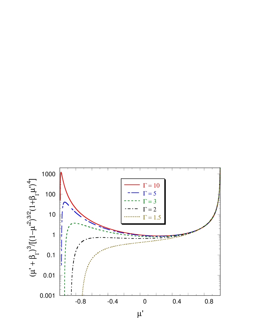
Figure 1: Integrand of integral on right-hand-side of equation (32).

Fig. 1 shows the integrand of the rightmost integral in equation (32). When $\Gamma\gg 1$, two dominant components of the differential energy density make up the total energy density: a component from the disk radiation field at disk radii $R\approx r$, called the near-field (NF) component; and a far field (FF) component coming directly from behind, which dominates the disk contribution at large radii (Dermer and Schlickeiser, 1993). The accretion disk radiation field, when approximated as a point source that illuminates the ejecta blob directly from behind, presents a total comoving energy density

$$u^{\prime}_{b}={1\over\Gamma^{2}(1+\beta_{\Gamma}^{2})^{2}}\;{3GM\dot{m}\over 8\pi cr^{2}R_{i}}\;(1-{2\over 3}\beta_{i})\;.$$ (33)

This result can be derived from the relation $u_{b}=2\pi\int_{0}^{\mu_{max}}d\mu\int_{0}^{\infty}d\epsilon(I^{\rm SS}_{\epsilon}/c)$, using equations (19) and (18) in the limit $r\gg R$, combined with the relativistic transformation of the energy density (eq.[6] in Dermer and Schlickeiser (1994)). The point-source approximation improves as the accretion disk looks more like a point source in the comoving frame, that is, when

$$\mu^{\prime}_{max}\cong{1-(R_{min}^{2}/2r^{2})-\beta_{\Gamma}\over 1-\beta_{\Gamma}(1-R^{2}_{min}/2r^{2})}\cong 1-2({\Gamma R_{min}\over r})^{2}\;\rightarrow 1.$$ (34)

The far-field approximation thus holds only when $r\gg\Gamma R_{min}$, and dominates the near-field component only when $r\gg\Gamma^{4}R_{min}$ (Appendix A.3). The following relationship connects the disk model with the disk radiant luminosity, neglecting advective effects:

$$L_{d}=2\times 2\pi\times\int_{R_{min}}^{\infty}dR\cdot R\cdot{dE\over dAdt}={3GM\dot{m}\over 2R_{i}}(1-{2\beta_{i}\over 3})\cong\;3^{-\beta_{i}}\,({GM\dot{m}\over 4r_{g}})\;.$$ (35)

In Appendices A1 and A2, analytic properties are derived of the integrand of the right-most term in equation (32) in the NF and FF limits, respectively.

9 Analytic Energy-Loss Rates and Spectra

This provides sufficient theory to derive expressions for radiation spectra in blazar jets. Simplified analytic expressions for electron-energy loss rates and spectral components are presented in the near-field and far-field regimes. For completeness, we also summarize results of our previous work for synchrotron and synchrotron self-Compton processes (Dermer and Schlickeiser, 1993; Dermer, Sturner, and Schlickeiser, 1997). These expressions employ $\delta$-function approximations for the emission spectra, and the spectral forms are least accurate near endpoints and spectral breaks.

9.1 Synchrotron Radiation

The rate at which a randomly ordered pitch-angle distribution of relativistic nonthermal electrons lose energy via the synchrotron process in a region with mean comoving magnetic-field intensity $B$ is given by $-m_{e}c^{2}\dot{\gamma}_{syn}$, where

$$-\dot{\gamma}_{syn}={4\over 3}\,{c\sigma_{\rm T}u_{B}\over m_{e}c^{2}}\,\gamma^{2}\cong 1.3\times 10^{-9}B^{2}\gamma^{2}\;{\rm s}^{-1}\;\equiv\;k_{syn}\gamma^{2}$$ (36)

(Blumenthal and Gould, 1970), and $u_{B}=B^{2}/8\pi$ is the energy density of the magnetic field.

In the $\delta$-function approximation for the elementary synchrotron emissivity, the $\nu F_{\nu}$ synchrotron radiation spectrum from a uniform blob, which is assumed to be spherical and to have a randomly oriented magnetic field in the comoving frame, is

$$f_{\epsilon}^{syn}\simeq\delta^{4}\;({c\sigma_{\rm T}u_{B}\over 6\pi d_{L}^{2}})\;\bar{\gamma}^{3}N_{e}(\bar{\gamma})\;,\;\bar{\gamma}=\sqrt{{(1+z)\epsilon\over\delta\epsilon_{B}}}\;.$$ (37)

In this expression, emission properties are integrated over variations on the comoving size scale of the plasma blob. On the corresponding observer time scale $t_{var}=(1+z)r_{b}/c\delta$, the blob upon reaching location $x$ is assumed to host an instantaneous electron energy spectrum $N_{e}(\gamma)$. Here $N_{e}(\gamma;x)d\gamma$ is the differential number of electrons with comoving Lorentz factors between $\gamma$ and $\gamma+$ d$\gamma$. $N_{e}(\gamma;x)$ is evaluated by solving a continuity or diffusion equation. Better descriptions of the system require integrations over the emitting volumes that arise from light-travel time effects (Chiaberge and Ghisellini, 1999; Chiang and Dermer, 1999; Granot et al., 1999).

9.2 Thomson-Scattered External Isotropic Monochromatic Radiation Field

Consider the Thomson energy-loss rate of electrons that are randomly distributed throughout a plasma blob that passes through a uniform external isotropic monochromatic radiation field with mean photon energy $\epsilon_{*}=10^{-4}\epsilon_{-4}$. The energy-loss rate due to Compton-scattered CMBR in the Thomson limit is given through

$$-\dot{\gamma}_{\rm T}={4\over 3}\;{c\sigma_{\rm T}\over m_{e}c^{2}}\gamma^{2}u_{*}\Gamma^{2}(1+\beta_{\Gamma}^{2}/3)\cong 3.3\times 10^{-8}u_{*}[{{\rm~{}ergs~{}}\over{\rm cm}^{2}}]\gamma^{2}\Gamma^{2}(1+\beta_{\Gamma}^{2}/3)\;{\rm s}^{-1}\;\equiv k_{\rm T}\gamma^{2}\;,$$ (38)

where $u_{*}$ is the energy density of the external isotropic radiation field photons which are scattered in the Thomson limit (Dermer and Schlickeiser, 1993, 1994). Equation (38) holds for $\gamma\ll\gamma_{\rm KN}$, where $\gamma_{\rm KN}$ is the Lorentz factor where Klein-Nishina (KN) effects become important, given through $4\gamma_{\rm KN}\Gamma\epsilon_{*}=1$. The transition from Thomson scattering to KN scattering takes place at observed photon energies $\epsilon_{\rm KN}\cong\delta/[16\Gamma\epsilon_{*}(1+z)]\cong 300(\delta/\Gamma)[\epsilon_{-4}(1+z)]^{-1}$ MeV (see Böttcher, Mause, and Schlickeiser (1997); Georganopoulos, Kirk, & Mastichiadis (2001), and Dermer and Atoyan (2002) for treatments of KN effects on external Compton scattering).

The $\nu F_{\nu}$ spectrum radiated by relativistic electrons which scatter photons from an external isotropic monochromatic radiation field in the Thomson limit is

$$f_{\epsilon}^{\rm T}\simeq\delta^{6}\;{c\sigma_{\rm T}u_{*}\over(p+3)\pi d_{L}^{2}}\;\bar{\gamma}^{3}N_{e}(\bar{\gamma})\;,\;\bar{\gamma}=\delta^{-1}\sqrt{{(1+z)\epsilon\over 2\epsilon_{*}}}\;$$ (39)

(Dermer, Sturner, and Schlickeiser, 1997). The mean ambient CMB photon energy $\epsilon_{*}=$ $\hat{\epsilon}(1+z)$, $\hat{\epsilon}\cong 2.7k_{\rm B}T_{CMB}/m_{e}c^{2}=$ $1.24\times 10^{-9}$, where $T_{CMB}=2.72$ K is the present temperature of the CMB, and $u_{*}=4\times 10^{-13}(1+z)^{4}$ ergs s^-1 is the local ambient CMBR energy density. For blazars, the ambient photon field might be reprocessed UV accretion disk radiation, with energy density depending on principle resonance line transitions in the broad line region or illuminated disk and torus. A simple prescription for the scattered radiation field is to let

$$u_{*}={L_{d}\tau_{sc}\over 4\pi r_{sc}^{2}c}=3.5\times 10^{-4}\,{\ell_{\rm Edd}M_{9}\over r_{sc}^{2}({\rm pc})}\;({\tau_{sc}\over 0.01})\;,\;{\rm where~{}}\;L_{d}=\ell_{\rm Edd}L_{\rm Edd}=\eta\dot{m}c^{2}{\rm~{}ergs}^{-1}\;,$$ (40)

$\tau_{sc}$ is an effective scattering depth of the surrounding medium including the broad line region, and $r_{sc}$ is the characteristic size of the surrounding scattering medium (Dermer and Schlickeiser, 1994). Effects of spatially varying external radiation energy densities from scattering media with power-law density gradients are treated by Blandford & Levinson (1995).

The distance along the jet axis beyond where the quasi-isotropic scattered radiation field arising, for example, from disk radiation scattered by broad emission-line clouds, dominates the point-source disk radiation field is $\cong 0.04R_{pc}\Gamma_{10}^{-2}(\tau_{sc}/0.01)^{-1/2}$ pc (Dermer and Schlickeiser, 1994). The appearance of weaker emission line fields in BL Lac objects suggests that accretion-disk rather than scattered soft-photon radiation could make a larger relative contribution to the SSC component in the inner jets of BL Lac objects, and this component should be included in detailed spectral models using more realistic accretion disk models. The radii where Thomson losses from the external scattered radiation field dominates the fields described in the NF and FF regimes are derived in Appendices A4 and A5, respectively. Appendix A6 describes different spectral states of blazars according to the dominant electron energy-loss processes. Appendix A7 considers the transition radius where the electron energy-loss rates from the CMBR field dominates those of the external accretion-disk radiation fields.

9.3 Thomson-Scattered Near-Field Accretion Disk Radiation Spectrum

Electrons lose energy when scattering soft photons of the accretion-disk radiation field. Considering an optically-thick Shakura and Sunyaev accretion disk radiation spectrum, the electron energy-loss rate in the Thomson limit of the near field ($r\approx R\gg 10r_{g}$) regime is given through

$$-\dot{\gamma}_{NF}\cong{4\over 3}\,c\sigma_{\rm T}\,[{0.7L_{d}\over 4\pi r^{2}c(m_{e}c^{2})}\,({r_{g}\over r})]\Gamma^{2}\gamma^{2}\;\equiv\;k_{NF}\;{\gamma^{2}\over\tilde{r}^{3}}\;.$$ (41)

The scattered $\nu F_{\nu}$ radiation spectrum for the near-field component of the disk field is

$$f_{\epsilon}^{NF}\simeq{1\over 2}\,\delta^{6}\,{c\sigma_{\rm T}\over 6\pi d_{L}^{2}}\;({L_{d}r_{g}\over 4\pi r^{3}c})\,\bar{\gamma}^{3}N_{e}(\bar{\gamma})\;,\;\bar{\gamma}\cong{\sqrt{2}\over\delta}\;\sqrt{{(1+z)\epsilon\over\bar{\epsilon}(\sqrt{3}r)}}\;.$$ (42)

The derivation of these results is found in Appendix B.

9.4 Thomson-Scattered Far-Field Accretion Disk Radiation Spectrum

Again considering an optically-thick Shakura and Sunyaev accretion disk radiation spectrum, the electron energy-loss rate in the Thomson limit of the far-field regime is given through

$$-\dot{\gamma}_{FF}\cong{4\over 3}\,c\sigma_{\rm T}\,[{L_{d}\over 4\pi r^{2}c(m_{e}c^{2})}]\;{\gamma^{2}\over\Gamma^{2}(1+\beta_{\Gamma})^{2}}\;\equiv\;k_{FF}\;{\gamma^{2}\over\tilde{r}^{2}}\;.$$ (43)

The scattered $\nu F_{\nu}$ radiation spectrum for the far-field component of the disk field is

$$f_{\epsilon}^{FF}\simeq\delta^{6}\,{c\sigma_{\rm T}\over 8\pi d_{L}^{2}}\;(1-\mu^{2})\;({L_{d}\over 4\pi r^{2}c})\,\bar{\gamma}^{3}N_{e}(\bar{\gamma})\;,\;\bar{\gamma}\cong{1\over\delta}\;\sqrt{{(1+z)\epsilon\over(1-\mu)\bar{\epsilon}(10r_{g})}}\;.$$ (44)

The derivation of these results is found in Appendix C. By comparing equations (41) and (43), we see that the transition from the dominance of the NF to the FF (point source) behavior occurs at the transition altitude $r_{tr}\approx 3\Gamma^{4}r_{g}$ (Dermer and Schlickeiser (1993); see Appendix A3).

9.5 Synchrotron Self-Compton Radiation

The energy-loss rate of electrons as they Compton scatter their self-synchrotron emission is, in the Thomson limit,

$$-\dot{\gamma}_{SSC,T}\simeq{4\over 3}\;{c\sigma_{\rm T}\over m_{e}c^{2}}\,[\int_{0}^{1/\gamma}\;u^{\prime}(\epsilon^{\prime})d\epsilon^{\prime}]\;\gamma^{2}$$ (45)

The spectral energy density can be directly related to observables through

$$\epsilon^{\prime}u^{\prime}(\epsilon^{\prime})\cong{2d_{L}^{2}\over r_{b}^{2}c}\;{f_{\epsilon}\over\delta^{4}}\;,\;\epsilon={\delta\epsilon^{\prime}\over(1+z)}\;{\rm and~{}}r_{b}\sim{c\delta t_{var}\over 1+z}\;,$$ (46)

where the last expression relates the comoving size scale to the variability time scale and redshift through $\delta$ (Tavecchio et al., 1998).

The $\nu F_{\nu}$ SSC spectrum in the $\delta$-function approximation for the synchrotron and Thomson emission spectra is

$$f_{\epsilon}^{SSC}\simeq{3\delta^{4}c\sigma_{\rm T}^{2}u_{B}\over 36\pi^{2}r_{b}^{2}d_{L}^{2}}\;({\epsilon^{\prime}\over\epsilon_{B}})^{3/2}\;\int_{\epsilon_{B}}^{{\rm min}(\epsilon^{\prime},1/\epsilon^{\prime})}d\epsilon^{\prime\prime}\;\epsilon^{\prime\prime-1}\,N_{e}[({\epsilon^{\prime\prime}\over\epsilon_{B}})^{1/2}]N_{e}[({\epsilon^{\prime}\over\epsilon^{\prime\prime}})^{1/2}]$$ (47)

(Dermer, Sturner, and Schlickeiser, 1997), where $\epsilon^{\prime}$ is related to $\epsilon$ in equation (46). Note that a factor $m_{e}c^{2}$ is missing in the calculation of the SSC spectrum in the paper by Dermer, Sturner, and Schlickeiser (1997), so that its importance is underestimated. Tavecchio et al. (1998) give expressions when the synchrotron spectrum is approximated by a broken power law.

10 Model for Blazar Variability

We operate in the regime where Thomson and synchrotron losses dominate SSC losses, adiabatic losses can be neglected, $B$ can be treated as constant, and processes involving external fields can be treated for the thermal accretion-disk model as considered in Section 9. The analytic solution presented below can also be extended to the cases where $B^{2}\propto r^{-2}$ and $B^{2}\propto r^{-3}$, though we only consdier a constant magnetic field in the calculations presented here. The neglect of Klein-Nishina effects on the electron energy loss rate and spectrum is a severe limitation of this model (see App. D). Accurate calculations employing realistic spectral forms for synchrotron and Compton processes are given in the papers by Böttcher, Mause, and Schlickeiser (1997), Böttcher (1999), Mukherjee et al. (1999), and Hartman et al. (2001).

In the stated approximations,

$$-\dot{\gamma}=[(k_{syn}+k_{T})+{k_{FF}\over\tilde{r}^{2}}+{k_{NF}\over\tilde{r}^{3}}]\gamma^{2}\;.$$ (48)

Location is specified in dimensionless units of $\tilde{r}=r/r_{g}$, $dt^{\prime}=r_{g}d\tilde{r}/(\beta_{\Gamma}\Gamma c)$, and the coefficients follow from the results of the previous section. Solving equation (48) gives

$$\gamma=\gamma(\gamma_{i},\tilde{r},\tilde{r}_{i})=[\gamma_{i}^{-1}+F(\tilde{r},\tilde{r}_{i})]^{-1}\;,$$ (49)

where

$$F(\tilde{r},\tilde{r}_{i})={r_{g}\over\beta_{\Gamma}\Gamma c}\;[(k_{syn}+k_{\rm T})(\tilde{r}-\tilde{r}_{i})+k_{FF}({1\over\tilde{r}_{0}}-{1\over\tilde{r}})+{1\over 2}k_{NF}({1\over\tilde{r}^{2}_{i}}-{1\over\tilde{r}^{2}})]\;,$$ (50)

where $r_{0}$ is the location at which the particle injection begins.

Within the framework of first-order Fermi acceleration theory, the injection spectrum of particles downstream of the shock is approximated by

$${dN^{\prime}_{e}(\gamma_{i})\over dt^{\prime}}=K\gamma_{i}^{-p}H[\gamma_{i};\gamma_{min},\gamma_{max}]\;,\;{\rm and~{}}K={(p-2)L_{e}^{\prime}\over m_{e}c^{2}(\gamma_{min}^{2-p}-\gamma_{max}^{2-p})}$$ (51)

where H[x;a,b] is a Heaviside function such that $H=1$ for $a\leq x<b$ and $H=0$ otherwise. The term $\gamma_{max}$ is determined by size scale, radiation, acceleration, available-time and kinematic limits (de Jager et al., 1996; Vietri, 1998; Rachen and Mészáros, 1998; Dermer and Humi, 2001). The normalization is easily made to the injection power into nonthermal electrons $L_{e}^{\prime}=dE^{\prime}_{e}/dt^{\prime}=dE_{*}/dt_{*}$, where the invariance of injection power between the stationary frame of the black-hole jet (starred) system and the comoving (primed) system is invoked. Hence the instantaneous electron spectrum at location $\tilde{r}$ is

$$N_{e}^{\prime}(\gamma;\tilde{r})={Kr_{g}\over\beta_{\Gamma}\Gamma c\gamma^{2}}\;\int_{\tilde{r}_{0}}^{\min[\tilde{r}_{1},\tilde{r}(t)]}\;d\tilde{r}^{\prime}\;\gamma_{i}^{2-p}\,H[\{\gamma^{-1}-F(\tilde{r}^{\prime},\tilde{r}_{i})\}^{-1};\gamma_{min},\gamma_{max}]\;.$$ (52)

The term $r_{1}$ is the location where particle injection ends, and $r(t)$ is the location of the jet that emits radiation observed at time $t$.

Equation (52) is easily solved using equations (49) and (50) to give the instantaneous electron spectrum in the approximation that $\Gamma$, $B$, and the injection power $L^{\prime}_{e}$ are constant with time. The allowed range of $\gamma$ is set by the Heaviside function and the limits on the integral, implying $\gamma>[\gamma_{min}^{-1}+F(\tilde{r},\tilde{r}_{0})]^{-1}$ for all values of $\tilde{r}\geq\tilde{r}_{0}$. When $\tilde{r}_{0}\leq\tilde{r}_{1}$, $\gamma<[\gamma_{max}^{-1}+F(\tilde{r},\tilde{r}_{0})]^{-1}$, whereas when $\tilde{r}\geq r_{1}$, $\gamma<[\gamma_{max}^{-1}+F(\tilde{r},\tilde{r}_{1})]^{-1}$. Mücke & Pohl (2000) were the first to modify the the approach of Dermer and Schlickeiser (1993) to extended injection. The methods of blast-wave physics (see, e.g., Mészáros, 2002) may be used to set $\gamma_{min}$ and $B$ and treat the spatial evolution of $\Gamma$ due to interactions with an external medium, at least in the adiabatic and fully radiative regimes. In this paper, we simply assign these values.

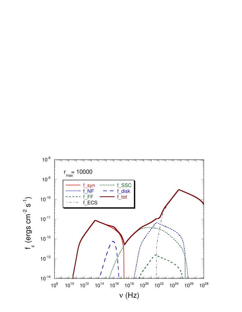
Figure 2: Spectral model of blazar variability, including an SSC component, and EC contributions from the direct near-field and far-field disk field and the quasi-isotropic scattered radiation field. Parameters and identification of the separate spectral components are given in the legend. (a) Electrons are uniformly injected with a comoving power of $1.26\times 10^{44}$ ergs s^-1 as the jet travels from $r=10^{3}r_{g}$ to $r=1500r_{g}$. (b) Same as in Fig. 2a, but with the electrons uniformly injected between $r=10^{3}r_{g}$ and $r=2000r_{g}$.(c) Same as in Fig. 2a, but with electrons uniformly injected between $r=10^{3}r_{g}$ and $r=4000r_{g}$. (d) Same as in Fig. 2a, but with electrons uniformly injected between $r=10^{3}r_{g}$ and $r=7000r_{g}$.(e) Same as in Fig. 2a, but with electrons uniformly injected between $r=10^{3}r_{g}$ and $r=10^{4}r_{g}$.

Fig. 2 shows the evolution of the spectral components in the toy model for a standard parameter set: $\Gamma=20$, $\theta=1/\Gamma$, $M_{9}=0.1$, $L_{\rm Edd}=1$, $\tau_{sc}=0.01$, $L_{e}=10^{44}$ ergs s^-1, $t_{var}=1$ day, $z=1$ ($d_{L}=2.4\times 10^{28}$ cm for a cosmology with 70% dark energy and a Hubble constant of 65 km s^-1 Mpc^-1), $B=1$ Gauss, $\gamma_{min}=10^{3}$, $\gamma_{max}=10^{5}$, $r_{sc}=0.1$ pc, and $p=2.3$. Because the electron power is small in comparison with the Eddington luminosity, the system could be accreting well below the Eddington limit, as argued in an evolutionary scenario by Böttcher and Dermer (2002). Different disk models appropriate to smaller values of the Eddington ratio can be treated in future work.

The injection is uniform between 1000 $r_{g}$ and 1500 $r_{g}$, 2000 $r_{g}$, 4000 $r_{g}$, 7000 $r_{g}$, and 10000 $r_{g}$ in Figs. 2a, 2b, 2c, 2d, and 2e, respectively. The relation $dr=\beta_{\Gamma}\Gamma c\delta dt/(1+z)$ implies

$$\tilde{r}_{3}\equiv{r(t)\over 1000r_{g}}=0.8\;{t_{4}\over M_{9}(1+z)}({\Gamma\over 20})^{2}\;({\delta\over\Gamma})\;,$$ (53)

where $t_{4}$ is the observing time in units of $10^{4}$ s, measured from the beginning of the flare when the emitting plasma was at $\tilde{r}_{0}$. For our standard values with $M_{9}=0.1$ and $z=1$, a $10^{4}$ s duration flare corresponds to the time during which the emitting blob travelling $4000r_{g}$.

This characteristic time scale is optimum for examining flares with GLAST in terms of flux levels for detecting intraday variability and proposed GLAST slewing strategies, as discussed in the next section. As can be seen in Fig. 2,, a dominant spectral feature from the near-field accretion disk component appears early in the flare, during which the $X/\gamma$ continuum is at a low lever. As the flare progresses, the near-field component becomes increasingly weak, and the bulk of the gamma-ray emission begins to originate from external scattered soft disk photons. The $\approx 10$ MeV - 1 GeV, X-ray and synchrotron radiations decline while the $>1$ GeV radiation monotonically increases. In addition to KN effects on the particle and photon spectra, the diffuse intergalactic infrared radiation field will attenuate $\gg 10$ GeV radiation. The important cosmological implications of this effect are discussed by, e.g., Primack et al. (1999) and Salamon & Stecker (1998).

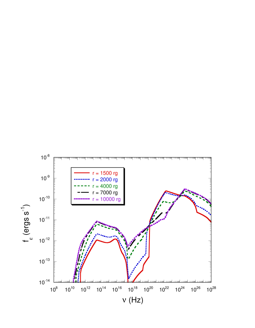
Figure 3: Multiwavelength variability behavior for a uniform injection event for the model in Fig. 2, beginning when the jet is at $r=10^{3}r_{g}$, and ending when $r=10^{4}r_{g}$. Note the decline of the direct disk-radiation field component with distance from the black hole.

Fig. 3 shows the evolution of the SED with distance from the black-hole core. For constant Lorentz factor $\Gamma=\delta=20$ and $M_{9}=0.1$, the duration of the episode from $10^{3}$ to $10^{4}r_{g}$ is 24 ksec. The pivoting behavior in the GLAST energy range is evident. Different injection profiles can change the the detailed behavior, but the discovery of $\gamma$-ray spectral components that individually vary in the manner described here would provide evidence for the interaction between the jet and the accretion-disk radiation field. At the earliest times in the flare, the actual disk field is apparent in the model spectrum at UV, EUV, and soft X-ray energies, and could be revealed from blazars at UV/soft X-ray energies during low-intensity states. The direct disk radiation from 3C 279 is argued to be detected when 3C 279 was faint in the UV (Pian et al., 1999).

The EC spectral component associated with the isotropic radiation field would apparently be absent or very weak in lineless or weakly-lined BL Lac objects, according to general understanding of these sources. In the scenario advanced by Böttcher and Dermer (2002) and Cavaliere & D’Elia (2002), BL Lac objects are AGN jet source at a stage in their life where the fueling is in decline and the black hole engine is most massive. When GLAST measures BL Lac blazars with better sensitivity, limits to the $\gamma$-ray flux of a disk radiation component in the 100 MeV - GeV range can be used to infer a relationship between the location of the acceleration and radiation sites in the jet in terms of $\delta$, which can itself be inferred from correlated X-ray and TeV $\gamma$-ray variability (Catanese et al., 1997) under the assumption that the X-rays and TeV $\gamma$ rays have a dominant origin in synchrotron and SSC processes, respectively. The near-field and far-field components have different antennae patterns, with the far-field component suppressed when observing very close along the jet axis (Dermer et al., 1992; Dermer and Schlickeiser, 1993).

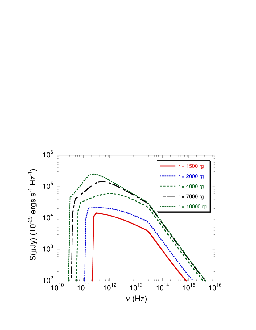
Figure 4: Flare profile presented as a flux density in units of micro-Janskys, showing the characteristic submillimeter/infrared behavior for this class of flare. The radio spectrum is not modeled here.

Fig. 4 displays the results of the considered model as a flux density in units of $\mu$Janskys. The rapid spectral evolution in the submillimeter is apparent, and can be tested with submillimeter and SIRTF observations of the flaring behavior of blazars. The radio spectrum is not modeled, and does not properly describe spectra at frequencies less than the mean synchrotron frequency $\langle\nu_{syn}\rangle=2\times 10^{6}B\delta\gamma_{min}^{2}/(1+z)$ Hz radiated by electrons with $\gamma=\gamma_{min}$. The model moreover breaks down below the synchrotron self-absorption frequency, which is not treated here. Proper modeling of radio requires a consistent treatment of adiabatic losses, which is also not done here. Böttcher (1999) points out that the radio spectrum varies differently in flat spectrum radio sources and BL Lac objects due to the dominance of the SSC processes in the latter class of sources.

If a $\gamma$-ray flare is a consequence of a relativistic plasma ejection event whereby the plasma becomes energized, either through an external or internal shock process as supposed in the model approach adopted here, then the delayed emergence of a radio-emitting blob is expected. Evidence for this behavior in EGRET data is presented by Jorstad et al. (2001). The quasi-continuous monitoring of $\gamma$-ray blazars with GLAST, in association with VLBI/SIM searches for superluminal motion in radio jet sources, will reveal whether $\gamma$-ray flares more typically precede or follow the emergence of radio blobs.

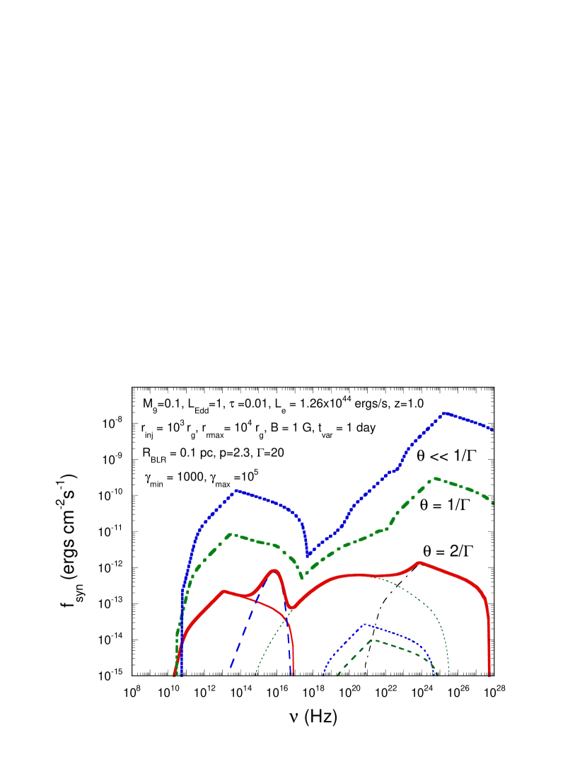
Figure 5: Angle-dependences of received $\nu F_{\nu}$ flux toy model blazar flare. The dominant Compton component at small angles reflects the different beaming factors of synchrotron, SSC and EC processes.

Fig. 5 shows the dependence on observing angle $\theta$ of the SEDs, for the continuous injection model where electrons are steadily injected during the period that the blob travels from $10^{3}$ to $10^{4}r_{g}$ (model 1e). Note the increasing dominance of the Thomson component over the synchrotron component at smaller observing angles $\theta$ due to the different beaming patterns of the two processes (Dermer, 1995; Dermer, Sturner, and Schlickeiser, 1997; Georganopoulos, Kirk, & Mastichiadis, 2001). Note also that the period of flaring activity for sources observed nearly along the jet is smaller than the interval over which the corresponding flux enhancements are observed at large angles to the jet axis. These effects are important in statistical treatments of flux-limited samples of blazar observed at different angles to the observer direction, which are assumed to be randomly oriented.

11 Blazar Flare Detectability with GLAST

We compare our model with the expected sensitivity of GLAST, noting that a recent estimate based on the phase 1 EGRET all sky-survey (Fichtel et al., 1994) shows that the rate at which GLAST will detect blazar flares sufficiently bright to detect $3\sigma$ variations on 1 hour time scales is about once per month (Dermer and Dingus, 2002).

11.1 Signal and Background in GLAST

The significance of blazar flare detection with GLAST is estimated (Thompson, 1986; Dermer and Dingus, 2002). The number of source photons with energies $E_{1}\leq E<E_{2}$ detected per unit observer time within the solid angle element $\Delta\Omega$ centered around a point source in the direction ($\theta(t),\phi(t)$) with respect to the normal of the face of the Large Area Telesccope (LAT) tower arrays at time $t$ is

$$\dot{S}\cong\int_{E_{1}}^{E_{2}}dE\;A[E,\theta(t),\phi(t)]\;\varphi_{s}(E,t)\;\{1-\exp[{-\Delta\Omega\over\Delta\Omega_{u}(E)}]\}\;,$$ (54)

where $\varphi_{s}(E,t)$ is the source photon flux (ph cm^-2 s^-1 E^-1), and $A(E,\theta,\phi)$ is the energy and angle-dependent effective area of GLAST. We assume that the scattered photons are distributed as a Gaussian with $\Delta\Omega_{u}(E)={9\over 4}\pi\theta^{2}_{u}(E)$ (Thompson, 1986), where $\theta_{u}(E)$ is the single photon angular resolution. This assumption can be checked against laboratory results to determine the angular response of the detector and amplitude of non-Gaussian wings in the point-spread function. The GLAST requirement for the single photon angular resolution (68% containment for on-axis sources) is $<3.5^{\circ}$ at 100 MeV and $<0.15^{\circ}$ at 10 GeV (GLAST Science Requirements Document, 2000). Hence $\theta_{u}=0.06(E/E_{100})^{-2/3}$, noting the inverse $2/3$ power of the energy dependence of the point spread function (Thompson, 1986; Fichtel and Trombka, 1997).

The source flux $\varphi_{s}(E,t)$ is related to the $\nu F_{\nu}$ flux $f_{E}($ergs s^-1) according to the relation $E\varphi_{s}(E,t)=f_{E}/E$. We characterize the $\nu F_{\nu}$ flux by a power law referred to 100 MeV (= $E_{100}$) photon energy. Thus

$$f_{E}\;=\;10^{-10}f_{-10}({E\over E_{100}})^{\alpha_{\nu}}\;{\rm~{}ergs~{}cm}^{-2}{\rm~{}s}^{-1}\;,$$ (55)

where $\alpha_{\nu}$ is the $\nu F_{\nu}$ spectral index.

The energy- and angle-dependent effective area of the GLAST LAT is approximated by the function

$$A(E,\theta)=A_{0}u(\theta)u(\theta)(E/E_{100})^{a(\theta)}\;,$$ (56)

where $u(\theta=0^{\circ})=1$, $a(\theta=0^{\circ})=a_{0}$, and azimuthal symmetry and time-independence of the detector effective area is assumed. An effective area derived from the successful GLAST LAT proposal is $A_{0}\approx 6200$ cm² and $a_{0}\approx 0.16$ for 100 MeV $\lesssim E\lesssim 10$ GeV. For 20 MeV $\lesssim E\lesssim 100$ MeV, $a_{0}\approx 0.37$. This satisfies the requirement for on-axis peak effective area of 8000 cm² in the 1-10 GeV range (GLAST Science Requirements Document, 2001). Hence the on-axis effective area $A\cong 6200(E/E_{100})^{a}$ cm², where $a=0.4$, $E<E_{100}$, and $a=0.16$, $E>E_{100}$.

Consider a source whose direction $\vec{\Omega}_{s}$ is precisely known. The number of background photons with energies $E$ between $E_{1}$ and $E_{2}$ detected per unit observer time within solid element $\Delta\Omega$ of the source direction is given by

$$\dot{B}\cong\Delta\Omega\int_{E_{1}}^{E_{2}}dE\;A[E,\theta(t),\phi(t)]\;\Phi_{B}(E,\vec{\Omega}_{s})\;.$$ (57)

The background flux per steradian is denoted by the term $\Phi_{B}(E,\vec{\Omega})$ (ph cm^-2 s^-1 sr^-1 $E^{-1}$) and is assumed to be time-independent. Considering only high-latitude sources where the extragalactic diffuse background radiation dominates all other sources of background radiation,

$$\Phi_{B}(E,\vec{\Omega})=K_{B}({E\over E_{100}})^{-\alpha_{B}}\;$$ (58)

(Sreekumar et al., 1998) in the range 70 MeV $\lesssim E\lesssim 10$ GeV, where $K_{B}=1.72(\pm 0.08)\times 10^{-7}$ ph (cm²-s-sr-MeV)^-1, and $\alpha_{B}=2.10\pm 0.03$.

An exposure factor $X$ is introduced that crudely takes into account source occultation and variation in detector effective area and photon localization with changing source direction of GLAST in its nominal slewing mode. For flaring behaviors detected on time scales less than the orbital time scale of 90 minutes ($t_{4}=0.54$), $X$ may approach 1. On longer time scales, $X\lower 2.15277pt\hbox{$\;\buildrel\rightarrow\over{\sim}\;$}0.2$. Hence

$$B\cong\Delta\Omega\Delta tXA_{0}K_{B}({E_{1}\over E_{100}})^{1+a-\alpha_{B}}\cdot 100\;{\rm MeV}\;\cong\;{12\over 1-0.4a}\;Xt_{4}({E_{1}\over E_{100}})^{a-2.43}\;,$$ (59)

where we let the solid angle acceptance for background $\Delta\Omega=\Delta\Omega_{u}$. The approximation in equation (59) takes into account that most of the background photons are collected at the lowest energy of the range of photon energies.

Similar approximations and simplications for the number of source counts [eq.(54)] gives the result

$$S\cong 19\;{Xt_{4}f_{-10}\over 1-{(a+\alpha_{\nu})\over 2}}\;({E\over E_{100}})^{-2+a+\alpha_{\nu}}\;.$$ (60)

The significance to detect a signal at the $n\sigma$ level for precisely known background is given by

$$n\cong{S\over\sqrt{B}}$$ (61)

(Li and Ma, 1983), where $S$ is the number of source counts and $B$ is the number of background counts.

Equations (59), (60), and (61) characterize high-latitude blazar detectability with GLAST, recognizing also that detection requires $S\gtrsim$ a few counts. At energies $E\gtrsim 100$ MeV, $a=0.16$, and we see that

$${S\over\sqrt{B}}\simeq{5\over 1-{\alpha_{\nu}\over 2.2}}\;\sqrt{Xt_{4}}f_{-10}\;({E\over E_{100}})^{\alpha_{\nu}-0.71}\;.$$ (62)

Detection of blazar sources is favored at $\approx 100$ MeV photon energies, except for the hardest sources with $\alpha_{\nu}\gtrsim 0.7$ (the mean flat spectrum radio quasar photon index in the 100 MeV - 5 GeV range observed with EGRET is $\langle\alpha_{\nu}\rangle\cong 0.2(\pm 0.2)$ (Mukherjee et al., 1997)). The decline in effective area and the increased background at lower energies start to hamper source detection efficiency with GLAST when $E\ll 100$ MeV.

11.2 Light Curves

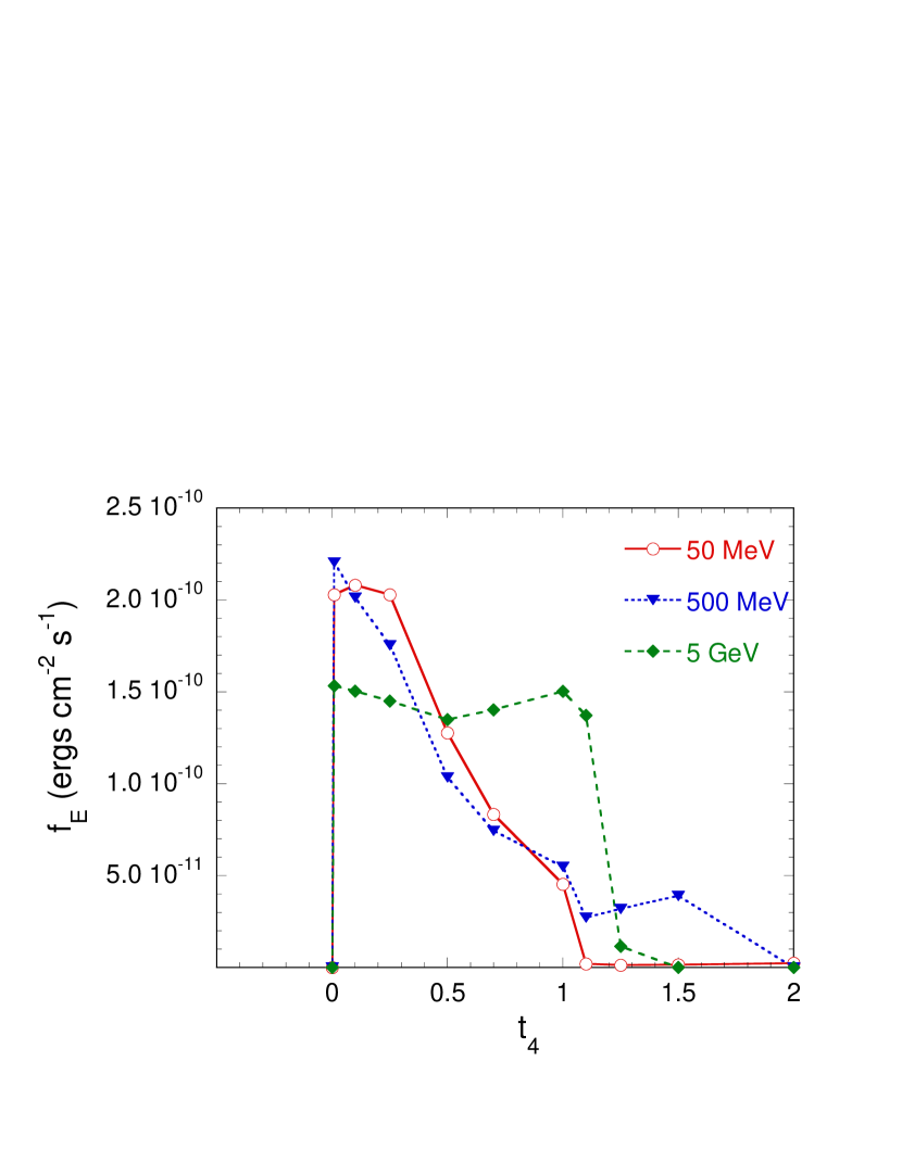
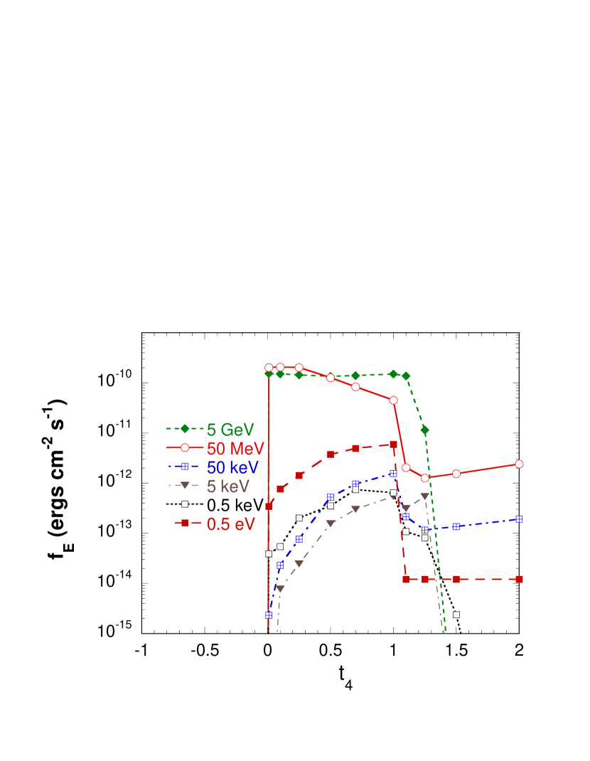
Figure 6: Light curves associated with a model flare where injection begins at $r=10^{3}r_{g}$ and ends at $r=5\times 10^{3}r_{g}$. Except for the time when particle injection stops, all other parameters are the same as in Fig. 2. Time is measured from the start of the flare in units of $10^{4}$ s. (a) Light curves at 50 MeV, 500 MeV, and 5 GeV. (b) Light curves at 0.5 eV, 0.5 keV, 5 keV, 50 keV, 50 MeV, and 5 GeV.

Light curves of the model blazar flare shown in Figs. 2-4 are plotted in Fig. 6, except that here the nonthermal electron injection ends at $r=5000r_{g}$. Aftter the radiating blob passes this location, there is no further injection and the nonthermal electrons cool only through radiative losses. Thus all three limits specified in the paragraph following equation (52) are relevant. The absence of adiabatic losses (see Sikora et al. (2001)), not to mention the assumptions about the constancy of $B$, $\Gamma$, etc., means that this result illustrates only a single limit of parameter space. The chief difference in our model from the recent work by Sikora et al. (2001) is the inclusion of the direct disk-jet component.

The high-energy light curves at $E=50$ MeV, 500 MeV, and 5 GeV are shown in Fig. 6a. The most notable feature is that the 5 GeV light curve continues to harden while the 50 MeV and 500 MeV light curves monotonically soften. This is a signature of a disk component fading as the blob travels outward, while the component from the scattered disk radiation persists at higher energies. The lower energy light curves in this figure reach a plateau after injection stops and electon cooling causes scattered accretion disk radiation to dominate in this waveband. The photon energy where the two components contribute equally depends, however, on disk parameters such as mass accretion rate and inner disk radius, and so might change for different model parameters.

Fig. 6b shows near infrared, X-ray, and medium energy $\gamma$-ray light curves. For this model, the synchrotron and SSC components are equal near 1 keV, and the synchrotron component dominates at lower energies. Consequently the 0.5 eV IR light curve abruptly declines after the acceleration episode ends. The X-ray flaring behaviors seen at 0.5 keV and 5 keV reflect the combined synchrotron and SSC decline after the injection stops. At 50 keV, the direct accretion-disk component causes a late time flattening in the light curve, similar to the behavior seen in the 50 MeV light curve, though the latter is due to the scattered accretion-disk component. Note also that these light curves will be smeared out if an integration over light travel time effects is made (Chiaberge and Ghisellini, 1999).

By comparing the blazar flare light curves at $\gamma$-ray energies with the expression for the significance of detection with GLAST, given by equation (62), one sees that the flaring behavior will be detectable, though spectral detail will be difficult to extract for the flux given by this model. The characteristic signature of a direct accretion disk component will be indicated in GLAST data by a soft-to-hard behavior at $\sim$ GeV energies compared to a hard-to-soft behavior at $\sim 100$ MeV energies.

12 Summary and Conclusions

In response to a query from Prof. Dr. John G. Kirk about the applicability of the optically thin approach used in DS93 to an optically-thick Shakura-Sunyaev accretion-disk spectrum, we have reexamined the basis and clarified the approach used in the paper by Dermer and Schlickeiser (1993) (a different approach is used in the paper by Dermer, Sturner, and Schlickeiser (1997)). An optically-thin formulation is used in the 1993 paper, which appears justified in the case of accretion-disk models with large radial flow speeds. For specificity, a photon energy corresponding to the blackbody value was used, though a wide range of choices may be treated. We conclude that the method is adequate to treat this special case.

Energy loss rates and spectral functions were derived in the Thomson regime for the cases of soft photons originating from an external isotropic monochromatic radiation field, and from a geometrically-thin accretion disk divided into near-field and far-field regimes in the limits $\Gamma\gg 1$ and $r\gg\Gamma r_{g}$ (Appendix A). SSC energy-losses were assumed to be small, and the SSC component was calculated in the Thomson regime. A simplified model was examined, and a characteristic variability pattern was identified whereby the near-field accretion disk component, initially bright at $\lesssim 1$ GeV energies, declines in intensity while the component formed by jet electrons that scatter photons of the external isotropic field becomes increasingly dominant at $\gtrsim 1$ GeV energies until particle injection stops. Campaigns organized around GLAST observations will be crucially important to interpret the jet-disk interaction by revealing the physical state of the jet with respect to the disk. The intensity of the thermal disk during the low state can additionally be inferred from optical, UV, and X-ray measurements of blazars during low-intensity states.

Both SSC and EC processes contribute to blazar $\gamma$-ray production, with a greater contribution of the internal power dissipated by external Compton (EC) emission in flat radio-spectra quasars, and a dominant SSC component in BL Lac objects. Multiple radiation components are required to model well-measured contemporaneous blazar spectra (Böttcher, 1999; Hartman et al., 2001; Mukherjee et al., 1999; Sikora et al., 2001). Spectral variations among different radiation components during different intensity states has been considered by Böttcher (2000). A characteristic optical/UV spectrum with $\alpha\cong 3/2$ is found for injection models with dominating SSC energy losses (Chiang and Böttcher, 2002). The present paper extends this work to provide an approach to model temporal variations of state transitions, though the treatment of SSC losses must be improved in future work.

Our model is very preliminary, and we have not even followed a complete flaring cycle. It is unlikely that the magnetic field remains constant over thousands or tens of thousands of $r_{g}$, and analytic models with $B^{2}\propto r^{-2}$ and $B^{2}\propto r^{-3}$, or numerical models with more general variations of $B$ remain to be considered, including the related adiabatic losses. The EC component from the soft scattered accretion-disk photons will also decline in intensity as the relativistic ejecta leaves the broad-line region. Adiabatic expansion will degrade particle energy until a dominant synchrotron component remains. The ejecta will expand, cool, decelerate, and on occasion be reenergized by internal or external shock interactions. The transition radius from the inner jet, where the external radiation field is dominated by either direct or scattered accretion-disk emissions, to the outer jet, where the external photon field is CMBR dominated, occurs on the kiloparsec scale for relativistic ejecta.

In the extended jet, the dominant radiation processes are nonthermal synchrotron radiation, SSC emission, and Compton-scattered CMBR (e.g., Harris and Krawczynski, 2002). Klein-Nishina effects can imprint the spectrum with a hardening in the Chandra range, as observed in the knots of 3C 273 (Marshall et al., 2001; Sambruna et al., 2001; Dermer and Atoyan, 2002). As the jet slows to nonrelativistic speeds at a terminal shock, either synchrotron or SSC process may dominate, as in the western hot spots of Pictor A (Wilson, Young, and Shopbell, 2001). Extended jet formation could be catalyzed by neutral beam production in the inner jet (Atoyan & Dermer, 2001, 2002). The same external-field transformations can be used to solve the problem of the radiation spectrum from the outer jet, as presented here for application to the inner blazar jet.

This paper provides a framework to treat many such problems involving different models and geometries of the accretion-disk radiation field in both the optically-thick and optically-thin limits, and for other external radiation fields. A simple extension of these results to incorporate advective effects on accretion is to change the inner boundary of the Shakura-Sunyaev disk to $\sim 100r_{g}$, within which a low-luminosity or nonradiating advection-dominated flow is found, with convection instabilities forming the jet. Application of these results to more complicated accretion-disk models, to photomeson production in blazars, and emission spectra in GRBs will be presented in subsequent work.

Appendix A Energy Loss Rates in the Near-Field and Far-Field Regimes

Consider equation (32),

$$u_{ext}^{\prime}={3GM\dot{m}\over 8\pi c\Gamma r^{3}}\;\int_{-\beta_{\Gamma}}^{\mu^{\prime}_{max}}d\mu^{\prime}\;{(\mu^{\prime}+\beta_{\Gamma})^{3}\over(1-\mu^{\prime 2})^{3/2}(1+\beta_{\Gamma}\mu^{\prime})^{4}}\;={3GM\dot{m}\over 8\pi cr^{3}\Gamma}(I_{NF}+I_{FF})\;,$$ (A1)

valid in the case $\beta_{i}=0$, implying an efficiency of 25% for this metric. We have divided the comoving energy density into a NF component, with $-\beta_{\Gamma}\leq\mu^{\prime}<0$, and a FF component with $0\leq\mu^{\prime}<\mu^{\prime}_{max}$.

A.1 Near-Field Integral

The expansion $\mu^{\prime}=-1+(N^{2}/2\Gamma^{2})$ in the near-field integral gives, in the limit $\Gamma\gg 1$,

$$I_{NF}=\int_{-\beta_{\Gamma}}^{0}d\mu^{\prime}\;{(\mu^{\prime}+\beta_{\Gamma})^{3}\over(1-\mu^{\prime 2})^{3/2}(1+\beta_{\Gamma}\mu^{\prime})^{4}}\;\;\;\lower 2.15277pt\hbox{$\;\buildrel\rightarrow\over{\Gamma\gg 1}\;$}\;\;\;2\Gamma^{3}c_{d}\;,$$ (A2)

where

$$c_{d}\equiv\int_{1}^{\infty}dN{(N^{2}-1)^{3}\over N^{2}(N^{2}+1)^{4}}\cong 0.023\;.$$ (A3)

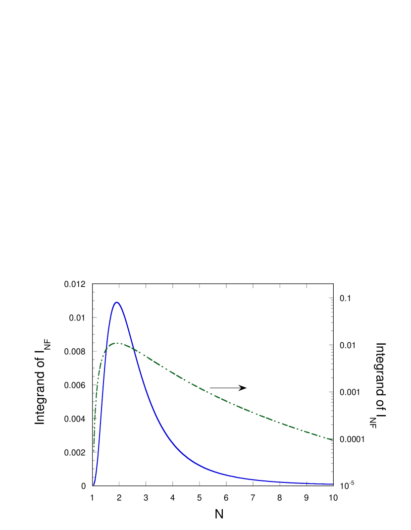
Figure 7: The integrand $(N^{2}-1)^{3}/[N^{2}(N^{2}+1)^{4}]$ of equation (A3).

This result agrees with the estimate $c_{d}\cong 2\times 3^{3}/(2^{2}\cdot 5^{4})=0.0216$, using the value of the integrand at $N=\Gamma\theta\cong 2$ (the integrand peaks at $\theta^{\prime}\cong 1.9/\Gamma$ in the limit $\Gamma\gg 1$). Fig. 7 presents the integrand of equation (A3).

A.2 Far-Field Integral

The far-field integral is

$$I_{FF}=\int_{0}^{\mu^{\prime}_{max}}d\mu^{\prime}\;{(\mu^{\prime}+\beta_{\Gamma})^{3}\over(1-\mu^{\prime 2})^{3/2}(1+\beta_{\Gamma}\mu^{\prime})^{4}}\;,$$ (A4)

and $\mu_{max}\cong 1-(R_{min}^{2}/2r^{2})$ in the limit $r\gg R_{max}$. Hence

$$\mu_{max}^{\prime}={\mu_{max}-\beta_{\Gamma}\over 1-\beta_{\Gamma}\mu_{max}}\;=\;1-2a^{2}+O(a^{2}/\Gamma^{2})\;,$$ (A5)

in the limit $a\equiv\Gamma R_{min}/r\ll 1$. Therefore

$$I_{FF}\;\;\;\;\lower 2.15277pt\hbox{$\;\buildrel\rightarrow\over{a\ll 1}\;$}\;\;\;\;{r\over 4\Gamma R_{min}}\;=\;{1\over 4a}\;.$$ (A6)

A.3 Near-Field/Far-Field Transition Radius

From equations (A1), (A2) and (A6),

$$u_{ext}^{\prime}={3GM\dot{m}\over 8\pi cr^{3}\Gamma}(2\Gamma^{3}c_{d}+{r\over 4\Gamma R_{min}}),$$ (A7)

implying for a Schwarzschild metric with $\beta_{i}=0$, the NF/FF transition radius

$$\tilde{r}_{NFFF}=\Gamma^{4}\;,$$ (A8)

in normalized units $\tilde{r}=r/r_{g}$.

A.4 Near-Field/Scattered Field Transition Radius

The location $r_{NX}$ where the NF equals the external scattered radiation field is given by the condition

$${3GM\dot{m}\over 8\pi cr^{3}\Gamma}\;\times\;2\Gamma^{3}c_{d}=u^{\prime}_{NF}=u^{\prime}_{sc}=\Gamma^{2}(1+\beta_{\Gamma}^{2}/3)u_{*}=\Gamma^{2}(1+\beta_{\Gamma}^{2}/3){L_{d}\tau_{sc}\over 4\pi r_{sc}^{2}c}\;.$$ (A9)

Recalling equation (35), we find

$$\tilde{r}_{NX}={r_{NX}\over r_{g}}=c_{d}^{1/3}\,3^{(2+\beta_{i})/3}\;{\tilde{r}_{sc}^{2/3}\over\tau_{sc}^{1/3}}\cong(0.59{\rm-}0.85)\;{\tilde{r}_{sc}^{2/3}\over\tau_{sc}^{1/3}}\;,$$ (A10)

where the coefficient varies in value as $\beta_{i}$ ranges from 0 to 1, and $r_{sc}=r_{g}\tilde{r}_{sc}$ is the characteristic size of the scattering region, which we identify with the broad-line region. Hence

$$\tilde{r}_{NX}\approx{\tilde{r}_{sc}^{2/3}\over\tau_{sc}^{1/3}}\;.$$ (A11)

Equation (A11) holds when $\tilde{r}_{NX}<\tilde{r}_{sc}$ for the simplified geometry of the scattering region assumed here, requiring that $\tilde{r}_{sc}>1/\tau_{sc}$. If $r_{sc}=0.5$ pc around a $10^{9}$ Solar mass black hole, then $\tilde{r}_{sc}=10^{4}$. The scattered radiation will dominate the NF radiation beyond $\approx 2000(\tau_{sc}/0.01)^{-1/3}r_{g}$ from the black hole.

A.5 Far-Field/Scattered Field Transition Radius

Equating equations (38) and (43) for the Thomson energy-loss rates of jet electrons by the quasi-isotropic scattered disk field and the far field limit of the accretion disk field, respectively, gives the location beyond which the direct disk field is no longer important. It is given by

$$\tilde{r}_{FX}\rightarrow{\sqrt{3}\over 4\Gamma^{2}}\;{\tilde{r}_{sc}\over\tau_{sc}^{1/2}}$$ (A12)

in the limit $\Gamma\gg 1$. Methods of reverberation mapping, normally applied to nearby radio-quiet Seyferts (e.g., Peterson, 1993), when applied to flat spectrum radio quasars with strong lines, such as 3C 273, 3C 279, PKS 0528+134, etc., can be used to infer $\tau_{sc}$ and the characteristic size $r_{sc}$ of the scattering clouds. A simple dependence of $r_{sc}$ on $r_{g}$ is unlikely, and furthermore, $r_{sc}$ may depend upon the spectral state and intensity of the accretion disk.

A.6 Intensity States of Extragalactic Relativistic Black-Hole Jet Sources

These considerations imply a variety of intensity states characterized by different relative values of

$$\tilde{r}_{NFFF}=\Gamma^{4}\;,\;\tilde{r}_{NX}\approx{\tilde{r}_{sc}^{2/3}\over\tau_{sc}^{1/3}}\;\;,\;\tilde{r}_{FX}={\Gamma^{-2}}\;{\tilde{r}_{sc}\over\tau_{sc}^{1/2}}.$$ (A13)

These relations hold within the framework of a geometrically thin, steady disk that radiates energy through viscous dissipation of gravitational energy in the absence of advective effects. Both the NF and the FF spectra are dominant at lower $\gamma$-ray energies than the external isotropic component. In fact, spectral breaks appear at $\approx\Gamma^{2}$ lower energy in the FF than the external isotropic component.

Flaring behaviors for flat spectrum radio quasars could involve transitions from the NF to the external scattered field, as modeled in Figs. 2-5. Weaker scattered radiation fields might also involve transitions from the FF to the external scattered field. In BL Lac objects, measurements of the intensity of scattered disk components with GLAST will restrict the distance from the black hole to the jet, given the specific accretion-disk model. Energy losses due to the SSC component must then be properly treated to identify the regime where BL Lac models operate. Modeling within the context of an ADAF scenario will improve predictive power and the value of this framework for the interpretation of multiwaveband observations of relativistic jet sources. This model is consistent with an evolutionary scenario where differences between classes of jet sources are a result of declining dust and gas (Böttcher and Dermer, 2002), and will be tested through statistics of flat spectrum quasars and BL Lac objects (Cavaliere & D’Elia, 2002).

A.7 Transition from the Inner Jet to the Extended Jet

A change in spectral state will occur when the pitch-angle averaged electron Thomson energy-loss rate due to external radiation fields begins to be dominated by the CMBR rather than the accretion-disk emission as a consequence of declining intensity of the accretion-disk field with distance. This occurs at the radius $r_{exj}$ given by

$${4\over 3}\Gamma^{2}\hat{u}_{CMB}(1+z)^{4}=\chi\;{L_{d}\over 4\pi r_{exj}^{2}c\cdot 4\Gamma^{2}}\;,$$ (A14)

where $\hat{u}_{CMB}=4\times 10^{-13}$ ergs cm^-3, and $\chi$ an amplification factor to be explained below.

We write the disk luminosity $L_{d}=\eta\dot{m}c^{2}=\ell_{\rm Edd}L_{\rm Edd}=1.26\times 10^{47}\ell_{\rm Edd}M_{9}$ ergs s^-1. Solving gives

$$r_{exj}=128\;{(\chi\ell_{\rm Edd}M_{9})^{1/2}\over\Gamma^{2}(1+z)^{2}}\;{\rm~{}kpc}\;\equiv r_{Xj}\;{\chi^{1/2}\over\Gamma^{2}}\;=320\;{(\chi\ell_{\rm Edd}M_{9})^{1/2}\over(\Gamma/10)^{2}[(1+z)/2]^{2}}\;{\rm~{}pc}$$ (A15)

The radius of the extended jet therefore begins on size scales of order kpc, though with wide variation depending strongly on $\Gamma$ and less strongly on the accretion-disk luminosity. The quantity $\chi$ represents directional amplification due to the relativistic inner jet. For the synchrotron component only (the $\gamma$-ray component would mostly be scattered by jet electrons in the KN limit), it seems possible that $\chi$ could reach values of 10 or more along the direction of the inner jet. Deceleration of the ejecta to nonrelativistic speeds in distant knots and hot spots would make possible the importance of the external Compton component from the inner jet, as defined by the quantity $r_{Xj}$. Thus the disk/inner jet radiation field could be important in spectral models of hot spots $\sim 10^{2}$ kpc from the central black hole when the accretion-disk or inner-jet power flares to $\sim L_{\rm Edd}$ over long time scales ($\gg 10^{3}$ yrs).

Appendix B Scattered Accretion-Disk Radiation Spectrum in the Near-Field Regime

From the analysis of the integrand of equation (A2) in the NF regime, we see that the NF photons originate from $\theta^{\prime}\cong 1.9/\Gamma$, or from $r\approx R$ in the stationary frame. From equations (35), (A1) and (A2), the comoving energy density in the NF regime is

$$u^{\prime~{}0}_{NF}={L_{d}\over 4\pi r^{2}c}\;4\cdot 3^{1+\beta_{i}}\;c_{d}({r_{g}\over r})\Gamma^{2}\;,$$ (B1)

and $4\cdot\ 3^{1+\beta_{i}}\;c_{d}=0.28,0.83$ when $\beta_{i}=0,1$, respectively. Taking the peak contribution from the disk at $\mu=1/2$, we have the following approximation for the comoving energy density:

$$u^{\prime}_{NF}={u^{\prime~{}0}_{NF}\over 2\pi}\;\delta(\epsilon^{\prime}-\Gamma\epsilon_{*}/2)\delta(\mu^{\prime}+1)\;.$$ (B2)

The comoving emissivity can be derived from

$$j^{\prime}(\epsilon^{\prime}_{s},\Omega^{\prime}_{s})=c\int_{0}^{\infty}d\epsilon^{\prime}\oint d\Omega^{\prime}\int_{1}^{\infty}d\gamma\oint d\Omega_{e}\;(1-\beta\cos\psi)({\epsilon^{\prime}_{s}\over\epsilon^{\prime}})u_{ph}^{\prime}(\epsilon^{\prime},\Omega^{\prime})n_{e}(\gamma,\Omega_{e})\;({d\sigma\over d\epsilon^{\prime}_{s}d\Omega_{s}})\;$$ (B3)

(Dermer, Sturner, and Schlickeiser, 1997), and $\cos\psi=\mu_{e}\mu^{\prime}+(1-\mu_{e}^{2})^{1/2}(1-\mu^{\prime~{}2})^{1/2}\cos(\phi_{e}-\phi^{\prime})$. Equation (B3) allows to examine the evolution of the particle distribution function in the comoving frame. An important simplifying assumption we make at this point is to assume isotropy of the electron distribution function in the comoving frame, that is,

$$n_{e}(\gamma,\Omega_{e})={n_{e}(\gamma)\over 4\pi}\;.$$ (B4)

For the cross section in the Thomson regime, we make the approximation

$${d\sigma\over d\epsilon^{\prime}_{s}d\Omega^{\prime}_{s}}=\sigma_{\rm T}\delta[\epsilon^{\prime}_{s}-\gamma^{2}\epsilon^{\prime}(1-\beta\cos\psi)]\delta(\Omega^{\prime}_{s}-\Omega_{e})\;.$$ (B5)

Solving gives

$$j^{\prime}(\epsilon^{\prime}_{s},\Omega^{\prime}_{s})={c\sigma_{\rm T}u^{\prime~{}0}_{NF}\over 2\pi}\;{(1+\mu^{\prime}_{s})^{2}\over 4\epsilon^{\prime}_{s}}\;\gamma_{NF}^{3}n_{e}(\gamma_{NF})\;\;,\;\;\gamma_{NF}=\sqrt{{2\epsilon^{\prime}_{s}\over\Gamma\epsilon_{*}(1+\mu^{\prime}_{s})}}\;.$$ (B6)

The $\nu F_{\nu}$ spectrum

$$f_{\epsilon}^{NF}={\delta^{4}\over d_{L}^{2}}\;V_{b}\epsilon^{\prime}_{s}j^{\prime}(\epsilon^{\prime}_{s},\Omega^{\prime}_{s})\;,\;\delta=[\Gamma(1-\beta_{\Gamma}\mu_{s})]^{-1}\;,\;.$$ (B7)

Making the transformation to observer frame quantities using the relation $1+\mu^{\prime}_{s}\rightarrow\delta(1+\mu_{s})/2\Gamma$, valid when $\Gamma\gg 1$, gives

$$f_{\epsilon}^{NF}={\delta^{6}c\sigma_{\rm T}u^{\prime~{}0}_{NF}\over 32\pi d_{L}^{2}\Gamma^{2}}\;(1+\mu_{s})^{2}\hat{\gamma}^{3}N_{e}(\hat{\gamma})\;,\;\hat{\gamma}={2\over\delta}\;\sqrt{{(1+z)\epsilon\over\epsilon_{*}(1+\mu_{s})}}\;,$$ (B8)

from which equations (41) and (42) follow. A value intermediate to 0.28 and 0.83 is assigned in equations (41) and (42).

Appendix C Scattered Accretion-Disk Radiation Spectrum in the Far-Field Regime

The point-source approximation for a monochromatic radiation field coming directly from behind the direction of jet motion is

$$u_{FF}(\epsilon,\Omega)={L_{d}\over 4\pi r^{2}c}\;{\delta(\mu-1)\over 2\pi}\;\delta(\epsilon-\bar{\epsilon})\;.$$ (C1)

Making use of the relations $\epsilon=\Gamma\epsilon^{\prime}(1+\beta_{\Gamma}\mu^{\prime})$, $\mu=(\mu^{\prime}+\beta_{\Gamma})/(1+\beta_{\Gamma}\mu^{\prime})$, and $\phi=\phi^{\prime}$ gives

$$u_{FF}^{\prime}(\epsilon^{\prime},\Omega^{\prime})={L_{d}\over 8\pi^{2}r^{2}c}\;{\delta(\mu^{\prime}-1)\delta[\epsilon^{\prime}-\bar{\epsilon}/\Gamma(1+\beta_{\Gamma})]\over\Gamma^{2}(1+\beta_{\Gamma}^{2})}$$ (C2)

Following the same procedure as in Appendix B gives

$$j^{\prime}(\epsilon^{\prime}_{s},\Omega^{\prime}_{s})={\sigma_{\rm T}L_{d}(1-\mu^{\prime}_{s})\over 32\pi^{2}r^{2}\bar{\epsilon}\Gamma(1+\beta_{\Gamma})}\;\hat{\gamma}n_{e}(\hat{\gamma})\;,\;\hat{\gamma}=[{\Gamma\epsilon^{\prime}_{s}(1+\beta_{\Gamma})\over\bar{\epsilon}(1-\mu^{\prime}_{s})}]^{1/2}\;,$$ (C3)

so that

$$f_{\epsilon}^{FF}=\delta^{6}\;{c\sigma_{\rm T}(1-\mu_{s}^{2})\over 8\pi d_{L}^{2}}\;({L_{d}\over 4\pi r^{2}c})\;\tilde{\gamma}^{3}N_{e}(\tilde{\gamma})\;,\;\tilde{\gamma}\equiv\delta^{-1}\sqrt{{(1+z)\epsilon_{s}\over(1-\mu_{s})\bar{\epsilon}}}\;,$$ (C4)

giving equation (44).

The accuracy of the expression for $j^{\prime}(\epsilon^{\prime}_{s},\Omega^{\prime}_{s})$ in equation (C3) can be checked by deriving the comoving electron energy-loss rate

$$-m_{e}c^{2}\dot{\gamma}=\oint d\Omega^{\prime}_{s}\int_{0}^{\infty}\;d\epsilon^{\prime}_{s}\;V^{\prime}_{b}j^{\prime}(\epsilon^{\prime}_{s},\Omega^{\prime}_{s})\;\;,\;{\rm when}\;\;V^{\prime}_{b}n_{e}(\hat{\gamma})=\delta(\hat{\gamma}-\bar{\gamma})\;,$$ (C5)

from which follows equation (43).

Appendix D Klein-Nishina Effects in Compton Scattering

Georganopoulos, Kirk, & Mastichiadis (2001) have derived an expression for the radiation spectrum produced by an isotropic distribution of electrons that Compton-scatters external soft photons with monochromatic dimensionless energy $\epsilon_{*}$ and energy density $u_{*}$ in the stationary frame. Slightly modified, their result is

$$f_{\epsilon}^{\rm KN}=\delta^{3}\;{3\sigma_{\rm T}u_{*}\over 16\pi d_{L}^{2}}\;[{\epsilon(1+z)\over\epsilon_{*}}]^{2}\;\int_{1}^{\infty}d\gamma_{*}\;{F(x)N(\gamma_{*}/\delta)\over\gamma_{*}^{2}}\;H[\gamma_{*};\delta\gamma_{1},\delta\gamma_{2}]\;,$$ (D1)

where

$$F(x)=[2x\ln x+x-1-2x^{2}+{(4\epsilon_{*}\gamma_{*}x)^{2}\over 2(1+4\epsilon_{*}\gamma_{*}x)}]\;H[x;{1\over 4\gamma_{*}^{2}},1]\;\;,\;\;{\rm and}\;\;x={\epsilon(1+z)\over 4\gamma_{*}^{2}\epsilon_{*}}\;$$ (D2)

This expression employs the head-on approximation for the Compton scattering process (Jones, 1968; Blumenthal and Gould, 1970). The comoving electron spectrum in the range $\gamma_{1}\leq\gamma\leq\gamma_{2}$ is given by $N(\gamma)$. Klein-Nishina effects become important when $\epsilon\gtrsim 1/[(1+z)\epsilon_{*}]$.

For a power-law electron distribution $N(\gamma)=V_{b}^{\prime}k_{e}\gamma^{-p}H[\gamma;\gamma_{1},\gamma_{2}]$, where $V^{\prime}_{b}$ is the comoving blob volume, they also derive an accurate form for the Thomson regime expression of the specific spectral power, given by

$$L_{\rm GKM}(\epsilon,\Omega)=\delta^{3+p}\;{V_{b}^{\prime}k_{e}c\sigma_{\rm T}u_{*}\over 8\pi\epsilon_{*}}\;({\epsilon\over\epsilon_{*}})\;$$ (D3)

$$\times\{(\gamma_{2}\delta)^{-(1+p)}[{\epsilon\over 4\epsilon_{*}(p+3)(\gamma_{2}\delta)^{2}}-{1\over 1+p}]+({\epsilon\over 4\epsilon_{*}})^{-(1+p)/2}\;{2\over(1+p)(3+p)}\}\;,$$ (D4)

and show that it reduces to the expression

$$L_{xT}(\epsilon,\Omega)=\delta^{p+3}\;{c\sigma_{\rm T}u_{*}\over\pi(p+3)}\;V^{\prime}_{b}k_{e}\;2^{(p-3)/2}\;({\epsilon\over\epsilon_{*}})^{(1-p)/2}\;$$ (D5)

when $p>-1$, $\epsilon\ll 4\delta^{2}\epsilon_{*}\gamma_{2}^{2}$, and $\gamma_{2}\gg\gamma_{1}$. The Thomson scattered $\nu F_{\nu}$ spectrum of an external isotropic and monochromatic radiation field was derived by Dermer, Sturner, and Schlickeiser (1997) and is given by

$$f_{\epsilon}^{xT}={\delta^{4+2\alpha}\over{\alpha+2}}\;{c\sigma_{\rm T}u_{*}\over 16\pi d_{L}^{2}}\;k_{e}V_{b}^{\prime}(1+z)^{1-\alpha}\;{(1+\mu)^{2+\alpha}\over\mu}\;({\epsilon\over\epsilon_{*}})^{1-\alpha}\;,$$ (D6)

where $\alpha=(p-1)/2$. Equation (D6) recovers equation (D5) in the limit $\mu\rightarrow 1$, though the term $2^{(p-3)/2}=0.71,0.84,$ and 1.0 for $p=2,2.5,$ and 3, respectively, in equation (D6), is replaced by $2^{p-1}/(p+1)=0.67,0.81,$ and 1.0 for $p=2,2.5,$ and 3, respectively, in equation (D5). The factor $(1+\mu)^{(2+\alpha)}/\mu$ follows from the range of scattered photon energies and angles in the comoving frame, and indicates that $\mu>0$ is the range of validity of the expression.

The approach of Georganopoulos, Kirk, & Mastichiadis (2001) avoids the need to transform scattered radiation spectra from the comoving to observer frames by directly transforming electron energy spectra to the stationary frame. This is useful in the case of specified comoving electron distributions. When calculating evolving electron spectra, the external radiation fields must be transformed to the comoving frame in order to derive the electron cooling rates. Furthermore, if the electron distribution is not assumed to be isotropic in the comoving frame, it is also simpler to treat the evolving energy and angle-dependent transformations of the electron spectra in the comoving frame. Whether one performs the scattering in the comoving frame and then transforms the radiation spectrum, or transforms the electron spectrum to the stationary frame and then performs the scattering, the final result must of course be the same.

Georganopoulos, Kirk, & Mastichiadis (2001) showed that the Thomson approximations (D4)-(D6) greatly overestimates the scattered radiation spectra compared to spectra calculated using equation (D1). This discrepancy is considerably reduced for electron spectra that evolve in response to Thomson losses in the Thomson-scattering approximation, compared with electrons that evolve under self-consistent Compton losses when using equation (D1). An approximate analytic treatment of KN losses and a detailed numerical treatment of joint Thomson and KN energy losses resulting from the CMBR field is performed by Dermer and Atoyan (2002), and Böttcher, Mause, and Schlickeiser (1997) calculate blazar spectra using the full Compton cross section.

References

- Arbeiter, Pohl, and Schlickeiser (2002) Arbeiter, K., Pohl, M., & Schlickeiser, R. 2002, A&A,386, 415
- Atoyan & Dermer (2001) Atoyan, A., & Dermer, C. D. 2001, Phys. Rev. Lett., 87, 221102
- Atoyan & Dermer (2002) Atoyan, A., & Dermer, C. D. 2002, in preparation
- Bednarek and Protheroe (1999) Bednarek, W., and Protheroe, R. J. 1999, MNRAS, 302, 373
- Blandford & Levinson (1995) Blandford, R. D., and Levinson, A. 1995, 441, 79
- Blazejowski et al. (2000) Blazejowski, M., Sikora, M., Moderski, R., and Madejski, G. M. 2000, ApJ, 545, 107
- Bloom & Marscher (1996) Bloom, S. D., & Marscher, A. P. 1996, ApJ, 461, 657