Long Term Variability of Cyg X-1

We present the long term evolution of the timing properties of the black hole candidate Cygnus X-1 in the 0.002–128 Hz frequency range as monitored from 1998 to 2001 with the Rossi X-ray Timing Explorer (RXTE). For most of this period the source was in its hard state. The power spectral density (PSD) is well modeled as the sum of four Lorentzians, which describe distinct broad noise components. Before 1998 July, Cyg X-1 was in a “quiet” hard state characterized primarily by the first three of these broad Lorentzians being dominant. Around 1998 May, this behavior changed: the total fractional rms amplitude decreased, the peak frequencies of the Lorentzians increased, the average time lag slightly increased, and the X-ray spectrum softened. The change in the timing parameters is mainly due to a strong decrease in the amplitude of the third Lorentzian. Since this event, an unusually large number of X-ray flares have been observed, which we classify as “failed state transitions”. During these failed state transitions, the X-ray power spectrum changes to that of the intermediate state. Modeling this PSD with the four Lorentzians, we find that the first Lorentzian component is suppressed relative to the second and third Lorentzian during the state transitions. We also confirm our previous conclusion that the frequency-dependent time lags increase significantly in the 3.2–10 Hz band during these transitions. We confirm the interpretation of the flares as failed state transitions with observations from the 2001 January and 2001 October soft states. Both the behavior of the PSD and the X-ray lag suggest that some or all of the Lorentzian components are associated with the accretion disk corona responsible for the hard state spectrum. We discuss the physical interpretation of our results.

1 Introduction

The existence of distinct states for the X-ray emission of black hole binaries (BHCs) has been extensively documented for many systems (see, e.g., Zhang et al. 1997a; Wilms et al. 2001; Homan et al. 2001). A geometrically thin, optically thick accretion disk is thought to be responsible for the soft, less variable X-ray flux dominating the soft state. In the hard state, an additional hot plasma, the “accretion disk corona”, is postulated to produce a hard, highly variable emission component which is in part reprocessed by the cooler disk. The hot plasma is also believed to be the reservoir for an outflow which emits synchrotron radiation at radio wavelengths (and possibly also in the X-rays, see Markoff et al. 2003 and references therein). While the general observational properties of BHCs are now well established (see, e.g, van der Klis 1995; Fender 2000; Remillard 2001), their unification in terms of a physical model is uncertain (Zdziarski 1999; Nowak et al. 2002). Especially, there exists no consistent model for explaining the complex short term variability on time scales faster than 1000 s, although several phenomenological models have been discussed (Böttcher 2001; Kotov et al. 2001; Poutanen 2002; Churazov et al. 2001; Nowak et al. 2002; Kazanas et al. 1997). These models explain the evolution and propagation of fluctuations in the X-ray flux in terms of several different mechanisms such as, e.g., infalling blobs of matter, development of localized X-ray flares, reflection, or wave propagation.

One of the possibilities to further improve current accretion models is to study the long term evolution of the canonical hard state, since in this state all the important physical components – disk, hot plasma, synchrotron outflow – as well as prominent short term variability can be observed. The stability of its characteristic parameters, however, has yet to be systematically studied with high spectral and temporal resolution. We therefore have performed regular monitoring observations of Cygnus X-1 with RXTE from 1998 to 2001. This persistent high mass X-ray binary (HMXB) is the best candidate for such a hard state campaign: it is bright ($\sim$0.6 Crab) and spends most of its time in the hard state. In addition to the canonical hard state properties, the 2–12 keV X-ray flux and the 15 GHz radio flux of Cyg X-1 display the 5.6 d orbital period and a 150 d period which might be due to precession of a disk/jet system (Pooley et al. 1999; Brocksopp et al. 1999a). The hard state shows weak and persistent radio emission that has been resolved as a type of steady jet (Stirling et al. 2001). The radio emission turns off during the soft state, as has been well documented during the last extended soft state which occurred from 1996 May to 1996 August (Zhang et al. 1997a; Cui et al. 1997, 1998; Wen et al. 2001).

The hard state PSD of Cyg X-1 has often been observed and modeled, the source serving as the BHC prototype. In addition to the flat-topped hard state noise, the occasional presence of low frequency noise on timescales longer than 1000 s and of a probably associated weak quasi-periodic oscillation (QPO) at $\sim$$0.04$ Hz has been reported (Angelini et al. 1994; Vikhlinin et al. 1994). Early descriptions of the flat-topped PSD attributed the variability to Poisson distributed X-ray flares (shot noise) and generally approached the PSDs as being due to a single broad-band process (Nolan et al. 1981; Lochner et al. 1991; Pottschmidt et al. 1998, see, however, Belloni & Hasinger 1990b). In recent years, however, it has become increasingly clear that the hard state PSDs of Cyg X-1 and other BHCs show several “breaks”, i.e., frequencies where the PSD steepens (Nowak et al. 1999a; Belloni & Hasinger 1990a, and references therein), and that this complex structure has to be described by multiple components (Smith et al. 1997; Berger & van der Klis 1998; Nowak 2000; Nowak et al. 2002; Belloni et al. 2002). Often, the basic component of such models is still a shot noise component (Poutanen 2002; Smith et al. 1997).

While on first sight the hard state PSD of Cyg X-1 is dominated by two distinct broad components (Gilfanov et al. 1999), strong indications were recently found that it can be described remarkably well with four broad noise components that yield the main contribution to the root mean square (rms) amplitude in the 0.001 Hz to 100 Hz range (Nowak 2000). Occasionally, narrow features representing QPOs are required. A previously observed “QPO” peak, detected near 1 Hz with $Q\sim 1$ and $\sim 10\%$ rms amplitude (Rutledge et al. 1999), can possibly be identified with one of the above mentioned broad components being very prominent. During transitions to and from the soft state, broader QPOs ($Q\sim 0.5$–1, 3–17% rms amplitude) between 3 and 13 Hz have been observed (Cui et al. 1997). As we find below, their parameters suggest that they correspond to the noise components in the hard state, with varying central frequencies and amplitudes. The normalization and flat-top break frequency – associated with the broad component that has the lowest characteristic frequency – have long been known to be anti-correlated (Belloni & Hasinger 1990b). In addition, the two lowest characteristic frequencies associated with broad components have been observed to be correlated (Gilfanov et al. 1999). This latter correlation was discovered by Wijnands & van der Klis (1999) by comparing the flat top break frequency with the broad hard state “QPOs”.

A four-peak deconvolution of hard state black hole PSDs is especially interesting in the context of the question of whether any of these BHC noise features have the same origin as the generally much narrower and faster QPOs seen in neutron star binaries (e.g., the so-called horizontal branch QPO and twin kHz QPOs; Wijnands & van der Klis 1999; Psaltis et al. 1999; Nowak 2000; van Straaten et al. 2002). The aim of our PSD fits is therefore to identify the main noise components and to characterize their evolution in order to provide new data for constraining accretion models.

In this work we concentrate on describing the variability properties of Cyg X-1 in terms of the power spectral density (PSD), the Fourier-frequency dependent X-ray time lags, and simplified spectral models. Our aim is to characterize the accretion flow in the hard state. The description of the X-ray spectra in terms of more sophisticated accretion disk corona models will be published in a separate paper (Gleissner et al. 2003). This paper is organized as follows: In Sect. 2 we describe our observing campaign, the data screening, the computation of the power spectra, and the procedure of fitting multiple Lorentzian profiles to the power spectra. We then present our results in Sect. 3, starting with the long term evolution of the power spectrum (Sect. 3.1), followed by a discussion of the failed state transitions (Sect. 3.2), the transition into the 2002 soft state (Sect. 3.3), and the behavior of the narrow Lorentzians (Sect. 3.4). In Sect. 4 we summarize our results.

2 Observations and Data Analysis

2.1 The RXTE Monitoring Observations of Cyg X-1

The RXTE data presented here were obtained with the Proportional Counter Array (PCA; Jahoda et al. 1996) and with the All Sky Monitor (ASM; Levine et al. 1996), using the pointed RXTE observation programs P30157 (1998), P40099 (1999), and P50110 (2000–2001). We used the standard RXTE data analysis software, FTOOLS, Version 5.0, to create lightcurves with a time resolution of $2^{-6}$ s (P30157) or $2^{-8}$ s (P40099, P50110) in multiple energy bands. The energy bands extracted for P30157 and P40099/P50110 present the closest match possible for the available data modes (see Table 1), and include the bands used in our analysis of the X-ray time lags (Pottschmidt et al. 2000, 2001). With a few exceptions noted below, the PSD analyses presented here were performed using summed lightcurves in the $\sim$2 keV to 13.1 keV energy range.

The P30157 data set (weekly monitoring in 1998 with a nominal exposure time of 3 ks per observation) is the same that was used previously for the study of the evolution of X-ray time lags (Pottschmidt et al. 2000, 2001) and the evolution of X-ray spectra (Smith et al. 2002). The data set P40099 (biweekly monitoring in 1999 with a nominal exposure time of 10 ks per observation) presented here has also been included in the time lag study of Pottschmidt et al. (2001). The P50110 data (biweekly monitoring with a nominal exposure time of 20 ks per observation) have not been published before. Starting in 1999, simultaneous observations at radio wavelengths performed with the Ryle telescope in Cambridge, U.K., are also part of the campaign. In addition, daily radio fluxes were obtained with the Ryle telescope.

For all observations, high resolution lightcurves and X-ray spectra were generated using standard screening criteria: a pointing offset of $<0\aas@@fstack{\circ}01$, a SAA exclusion time of 30 minutes, and a source-elevation of $>10\degr$. At times of low source luminosity, when the “electron ratio”, i.e., a measure for the particle background in the PCA, was not influenced by the source itself, we also imposed a maximum “electron ratio” of 0.1. Good-time intervals (GTIs) were then created for all available PCU combinations, and from those suitable GTIs were selected for extracting high time-resolution data for the data modes and energy bands given in Table 1. For each GTI file, we generated the background spectrum using the FTOOL pcabackest and the “sky-VLE” background model. The background in a given energy band was then taken into account in determining the PSD normalization.

As a result of the data screening, $\sim$2 ks of usable data were left for each of the P30157 observations and $\sim$7 ks for P40099 and P50110. Note that due to RXTE scheduling constraints the full nominal exposure time was only rarely reached. Observation dates and exposure times are included in Table 2. The table caption given here contains a description of all parameters, the full table is available in electronic form at EDP Sciences.

Table 1: Energy bands and data modes used.

	PSD	lag/coherence
		low	high
PCA Epoch 3: data taken until 1999 March 22
data mode B_16ms_46M_0_49_H
channels	0–35	0–10	23–35
energy [keV]	$\sim$2–13.0	$\sim$2–4.2	8.3–13.0
PCA Epoch 4: data taken after 1999 March 22
data mode B_2ms_8B_0_35_Q
channels	0–30	0–10	20–30
energy [keV]	$\sim$2–13.1	$\sim$2–4.6	8.4–13.1

2.2 Computation of the Power Spectra

The computation of the power spectra for all energy bands given in Table 1 follows Nowak et al. (1999a) and Nowak (2000).

For the P30157 data set, PSDs in the 0.002 to 32 Hz range were computed, while the P40099 and P50110 PSDs reach up to 128 Hz. This discrepancy arises from the different maximum time resolutions of the binned data modes that are available for these data sets (see Table 1). We decided to use the binned modes with their comparatively moderate time resolutions, because they allow us to study several different energy bands (see Sect. 3.2) which cannot be done with the “single bit” data modes (250 $\mu$s time resolution) that are also available.

All PSDs used in this paper are presented in the normalization of Belloni & Hasinger (1990b) and Miyamoto et al. (1992), where the PSD integrated over a certain frequency interval equals the square of the relative contribution of that frequency interval to the total rms noise of the source. Where possible, we adjusted the normalization to the background corrected count rate. The observational deadtime corrected Poisson noise was subtracted before the normalization. See Vikhlinin et al. (1994) and Zhang et al. (1995) for a discussion of the deadtime influence on the PSD in general, Jernigan et al. (2000) and Zhang et al. (1996) for the case of the PCA detector, and Revnivtsev et al. (2000) for an application to PCA measurements of Cyg X-1 above 100 Hz. For most observations we used the first two components of Eq. (6) of Jernigan et al. (2000), namely the approximation of the “general paralyzable deadtime influence” (Zhang et al. 1995, Eq. (24)) plus the deadtime caused by “Very Large Events” (characterized by the PCA VLE count rate). For frequencies $<$100 Hz the correction of the noise level due to these two components amount to only a few percent. Higher order corrections or a fit of these components to the PSDs as applied by Jernigan et al. (2000) or Revnivtsev et al. (2000) are therefore not necessary here. We note that the discussed features in the PSDs have rms amplitudes well above the typical deadtime structures (see, e.g., Fig. 5 of Jernigan et al. 2000 or Fig. 4 of Revnivtsev et al. 2000).

A slightly different PSD normalization and deadtime correction has been applied to all observations performed after 2000 May 12, when the epoch of enhanced PCU 0 background count rates started. Here, a good background model was not yet available and thus we could not background correct the PSDs. This correction is only on the order of a few percent and does not influence appreciably our results (we note that this problem is, however, a serious problem for sources with a low count rate; Kalemci et al. 2001). Furthermore, as we do not have access to the VLE count rates from individual PCUs, it becomes impossible to correct the PSD for the VLE specific deadtime. Therefore, we only applied the general paralyzable deadtime correction.

For each observation we created three PSDs by averaging the individual PSDs from lightcurve segments with durations of 512 s, 128 s, and 32 s. Logarithmic frequency rebinning was performed on the same frequency grid for each of the three resulting PSDs. This grid ranges from $2^{-9}$ to $2^{5}$ (or $2^{7}$) Hz ($\sim$0.002 to 32 [or 128] Hz), with different d$f/f$ values for different frequency ranges: 25 logarithmically spaced bins were used from 0.001 Hz–0.1 Hz, 50 bins from 0.1–20 Hz, and 5(15) bins from 20–32(128) Hz. The final PSD was then created by selecting for each grid bin the highest signal to noise value among the three PSDs.

Figure 1: a) Best fit (solid line) to a typical 0.002–128 Hz hard state power spectrum of Cyg X-1 (P40099/18, 14off, 1999 September 13, diamonds) using multiple Lorentzians. The fit was performed for the energy range from $\sim$2 to 13.1 keV. It includes four broad (dashed lines) plus two narrow (dash-dotted lines) Lorentzian profiles and a power law component (dotted line). b) The same as above but here the PSD has been multiplied by frequency to illustrate the peak frequencies of the broad noise components (see Sect. 4 for a discussion of the importance of these frequencies). c) Residuals between data and model in units of the standard deviation of the PSD data.

Figure 2: a–c) Another typical fit, in this case to one of the P30157 observations (No. 11, 1998 February 20) in the 0.002–32 Hz frequency range. The best fit consists of four broad and one narrow Lorentzian profiles.

2.3 Modeling the Power Spectra

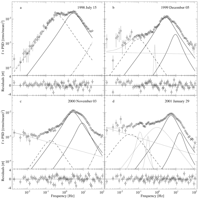
As was shown by Nowak (2000), multiple Lorentzian profiles can provide a good description of the typical hard state variability of Cyg X-1 and GX~339$-$4 in the 0.001–100 Hz range. Inspired by this success, we applied multiple Lorentzian profiles to model the PSDs from our monitoring campaign and generally obtained good fits (see Table 2 and the typical examples displayed in Fig. 1 and Fig. 2). Note that power spectra obtained during the soft state, e.g., during the 1996 soft state, are not well fit with the multi-Lorentzian model (see also Sect. 3.2 below). Our fitting approach uses standard $\chi^{2}$ minimization with the uncertainty of the free fit parameters determined using the usual prescription of Lampton et al. (1976). Unless noted otherwise, we give the uncertainty in terms of $1\sigma$ errors.

We describe the power spectra as the sum of Lorentzian profiles of the form

$$L_{i}(f)=\pi^{-1}\frac{2R_{i}^{2}Q_{i}f_{i}}{{f_{i}}^{2}+4Q_{i}^{2}(f-f_{i})^{2}}$$ (1)

where $f_{i}$ is the resonance frequency of the Lorentzian, $Q_{i}\sim f_{i}/\Delta f_{i,\text{FWHM}}$ its quality factor, and $R_{i}$ its normalization constant. Note that our definition of $Q$ is consistent with the common use of the $Q$-value (e.g., Belloni et al. 2002), but differs from that used by Nowak et al. (1999a) and Nowak (2000) where $Q=f_{i}/\Delta f_{i,\text{HWHM}}$ with $\Delta f_{i,\text{HWHM}}=\Delta f_{i,\text{FWHM}}/2$ was used.

Integrating this profile over the frequency range from zero to infinity gives its total rms amplitude:

$$\text{rms}_{i}=R_{i}\left(\frac{1}{2}-\frac{\tan^{-1}(-2Q_{i})}{\pi}\right)^{1/2}$$ (2)

A further important quantity of the Lorentzian is its peak frequency, i.e., the frequency where its contribution to the total rms variability is at its maximum:

$$\nu_{i}=f_{i}\left(1+\frac{1}{4Q_{i}^{2}}\right)^{1/2}$$ (3)

As it was recently found that $\nu_{i}$ seems to be the important parameter in terms of frequency correlations (Nowak 2000; Nowak et al. 2002; van Straaten et al. 2002; Belloni et al. 2002), we will use $\nu_{i}$, and not $f_{i}$, to describe the location of each Lorentzian, unless specifically noted otherwise.

Table 2: Results of fitting multiple Lorentzians to selected power spectra of the Cyg X-1 RXTE/PCA monitoring observations from 1998–2001 in the frequency range from (1/512) Hz to 32 Hz (P30157) or 128 Hz (others), for the 2–13 keV band (Table 1). The table is available in electronic form via http://www.edpsciences.org. Apart from the fit results, it contains the following information for each observation: running number, proposal name (e.g., “P40099”), sub-ID within the proposal, PCUs turned off, date of the observation, and the exposure time in ks. The fit results for each observation are organized as follows: for each of the possible four broad and three thin Lorentzians the norm ($R$), central frequency ($f$), and quality factor ($Q$) with their corresponding uncertainties are listed. In addition the power law normalization ($A$) and slope ($\alpha$) are given if present in the model. Finally, the $\chi^{2}/{\text{dof}}$ and $\chi^{2}_{\text{red}}$ values of the fit are listed.

Alternative models for the lowest frequency Lorentzian, such as using a zero centered Lorentzian, i.e., a shot noise component featuring a single relaxation time scale (Belloni et al. 2002), may in principle provide fits of comparable quality (note that in the case of the observation analyzed by Nowak 2000, a zero centered Lorentzian provided a significantly worse fit). The multi-Lorentzian fits, however, provide the most uniform description as well as the possibility to compare the noise components with those found in neutron star binaries (see Sect. 4).

In almost all of our PSDs, four broad Lorentzians are apparent (Figs. 1 and 2) which we call $L_{1}$, $L_{2}$, $L_{3}$, and $L_{4}$. The fourth broad component, $L_{4}$, is usually present above 32 Hz and has also been noted by Revnivtsev et al. (2000) and Nowak (2000). This component is also seen in other black hole or neutron star sources (van Straaten et al. 2002; Belloni et al. 2002). In the P30157 data set only its low frequency part can be seen. However, with the knowledge from the P40099 and P50110 data sets, we constrained its shape, especially its approximate width, and included this component in the P30157 models. We will discuss the issue of possible systematic errors resulting from this approach later.

We generally achieved a good fit using four broad Lorentzian components, $L_{1}$–$L_{4}$, with typical peak frequencies of $\sim$0.2 Hz, $\sim$2 Hz, $\sim$6 Hz, and $\sim$40 Hz. In our first modeling attempts we left the $Q$-factors of the Lorentzians as free parameters. They were found to vary considerably from observation to observation: $Q_{1}$, $Q_{2}$, and $Q_{3}$ ranged from $\sim$0.1–2.8, $Q_{4}$ was even less constrained. However, later experiments showed that fixing each $Q$-value to a representative value for each broad component does not significantly alter the fit results. This can be expected, since the broad components overlap over large frequency intervals (Figs. 1b and 2b). We therefore set $Q_{1}=0.25$, $Q_{2}=0.3$, $Q_{3}=0.3$, and $Q_{4}=0.5$ for all fits. This resulted in a good description of most PSDs. There are only 22 cases out of the total 130 PSDs where the fit significantly improved when one or more of the $Q$-factors were treated as a free parameter. In these cases, which mainly coincided with the “failed state transitions” further discussed in Sect. 3.2 below, we accepted the model with a variable $Q$ as the best fit. For the low signal to noise energy resolved PSDs of the P30157 data we fixed $Q_{4}$ and $f_{4}$ to their best-fit value of the non energy resolved PSD.

In addition to $L_{1}$ through $L_{4}$, a power law of the form

$$\text{PL}(f)=R_{\text{pl}}f^{-\alpha_{\text{pl}}}$$ (4)

is required in $\sim$40% of the observations. The majority of these power laws are required to reduce the residuals below $\sim$0.01 Hz. They have a typical slope of $\sim$1.3 and a normalization of $\sim$$10^{-4}$. In some instances the power law is the main contributor to the total rms amplitude. As we show in Sect. 3.2, these observations mainly coincide with “failed state transitions”. Generally, these observations are the same where we also had to leave the $Q$-values of the Lorentzians a free parameter. This can be expected as the contribution of the power law at higher frequencies slightly contaminates the other fit parameters. In other observations – normally those close to the “failed state transitions” – a clear deviation from the fit with broad Lorentzians is also present at low frequencies. Due to the logarithmic binning of our data, in these cases the deviations were quite often only seen in the lowest few frequency bins and thus there was not sufficient information to reliably constrain the shape of the deviation. For consistency with the fits performed for the “failed state transitions”, we chose to describe these observation with the same PSD model that we also used for the intermediate or soft state, thus implying that the reason for the low-frequency excess in these observations is the same as that for the excess during the “failed state transitions”. Since the uncertainty of the power law slope is rather large or undeterminable due to numerical reasons for these latter observations, we do not give specific uncertainties. We also caution that the difficulty in constraining the power law also results in an anti-correlation between $\alpha_{\text{pl}}$ and the power law normalization $R_{\text{pl}}$, which we view as being largely systematic in nature.

In agreement with Nowak (2000), Nowak et al. (2002), and Belloni et al. (2002), we often see additional subtle but statistically significant substructures. Sometimes these structures are sharp (Figs. 1 and 2) or weak and broad. In this case, further Lorentzian components ($L_{\text{add},i}$) were added to the basic PSD continuum. We generally retained these components if their addition resulted in a significant improvement of the best fit $\chi^{2}$, or if they were very clearly present in the PSDs. Residuals at frequencies slightly higher than the peak frequency of $L_{1}$ tended to be narrow. We modeled these features with one or two narrow Lorentzians, $L_{\text{add},1}$ and $L_{\text{add},2}$ (see Fig. 1 and Fig. 2). Typical peak frequencies for these QPOs range from 0.1 to 0.6 Hz, and one might speculate about their relationship to the horizontal branch oscillation peaks in neutron star X-ray binaries (Wijnands & van der Klis 1999, Table 4). In addition, below $L_{1}$ a broad, weak ($\lesssim 2\sigma$) residual at $\sim$0.03 Hz was often seen, which we designate $L_{\text{add},3}$. The total contribution of $L_{\text{add},1}$, $L_{\text{add},2}$, and $L_{\text{add},3}$ to the rms is on the order of a few percent at most. See Sect. 3.4 for a discussion of the behavior of these additional components.

Using this modeling approach, we obtained values for the reduced $\chi^{2}$ in the range of 1–2. The best-fit parameters of all 130 observations are given in electronic form in Table 2. Most of the remaining systematic residuals in these fits are probably due to the fact that the broad noise components have a more complex shape than a simple Lorentzian profile and/or that sub-harmonics are present. This is especially true for $L_{2}$, which is often associated with $\lesssim$$2\sigma$ residuals in the $\sim 1$–$2$ Hz range (see also Nowak 2000). The broad low-frequency residual $L_{\text{add},3}$ and other residuals at frequencies below $\nu_{1}$ might also be due to this effect. A further source of weak systematic residuals might be our choice of fixed $Q$-factors.

After obtaining the final best fit we computed the total rms variability amplitude relative to the mean count rate by summing the contributions of all power spectral fit components. The best fit Lorentzian profiles were integrated from zero to infinity (Eq. (2)), while the power law contribution was obtained by integrating the power law over the frequency range from $10^{-3}$ Hz to 200 Hz. Because of the different time resolution of the extracted lightcurves this approach is more systematic than the direct measurement of the rms variability from the X-ray data.

2.4 Time Lags, Coherence, and Spectral Modeling

Although the emphasis of this paper is on the evolution of the short term timing properties of Cyg X-1 in terms of the PSD, it is obviously important to also characterize the source in terms of other quantities.

For black hole candidates, the X-ray lightcurves in two energy bands are similar to each other. However, the X-ray lightcurve in a higher energy band generally lags that measured in a lower energy band. This X-ray time lag depends on the Fourier frequency. A measure for the similarity of the X-ray lightcurves in these two bands is given by their coherence, which is again Fourier frequency dependent. We compute both quantities using the formulae given by Nowak et al. (1999a). As we have shown previously, an especially interesting quantity is the average X-ray time lag in the 3.2–10 Hz band (Pottschmidt et al. 2000), which we will use to quantify the X-ray lag.

To obtain a description of the X-ray photon spectrum, we describe each source spectrum as the sum of a power law spectrum with photon index $\Gamma$ and a multi-temperature disk-black body after Makishima et al. (1986), characterized by the temperature at the inner edge of the accretion disk, $kT_{\text{in}}$. To this continuum, a reflection spectrum after Magdziarz & Zdziarski (1995) is added. For this paper we concentrate on the X-ray spectrum below $\sim$20 keV by ignoring the HEXTE data. Such an empirical model is sufficient to roughly describe the most important spectral parameters. A full study of the evolution of the broad-band X-ray spectrum that includes the HEXTE data and models the source spectrum in terms of the Comptonization models of Dove et al. (1997), Coppi (1999), and Poutanen & Svensson (1996) will be presented in a forthcoming paper (Gleissner et al. 2003).

3 Evolution of the Power Spectrum

Figure 3: Spectral and timing parameters of Cyg X-1 between 1997 and 2001. a) Photon index. b) X-ray time lag between 2–4 keV and 8–13 keV, averaged over the 3.2–10 Hz frequency band. c) X-ray coherence between 2–4 keV and 8–13 keV, averaged over the 3.2–10 Hz frequency band. d) Relative rms amplitude for the total 2–13.1 keV power spectrum. e) Relative rms amplitude and f) frequency of each of the four broad noise components. Crosses: $\text{rms}_{1}$, diamonds: $\text{rms}_{2}$, circles: $\text{rms}_{3}$, triangles: $\text{rms}_{4}$. g) Daily averaged 15 GHz radio flux, determined with the Ryle telescope. h): RXTE ASM 2–12 keV count rate. The dotted vertical lines mark special observations discussed in Sect. 3.2 and Sect. 3.3. The radio flux and the ASM rate have been rebinned to a resolution of $\sim$5.6 d, the orbital period of Cyg X-1, for clarity.

Figure 4: a) RXTE-PCA count rate (2.5–20 keV) for each pointing, as well as b) RXTE-ASM count rate and c) 15 GHz radio flux, both binned to a resolution of 1 d to show the variability on timescales that are smaller than the orbital timescale.

Table 3: Average values and standard deviations of the rms amplitudes, $\text{rms}_{i}$, the peak frequencies, $\nu_{i}$, and the frequency ratios, $\nu_{i}/\nu_{j}$, for the four broad noise components ($i,j=1,\ldots,4$). The values are derived for different time episodes surrounding the 1998 May change and the 1998 July failed state transition. For the P30157 data the highest peak frequency, $\nu_{4}$, is biased (see text) and is therefore not quoted in this table.

	P30157	P30157	P30157	P30157	P40099/P50110b
	(1–18)a	(19–28)	(29–32)	(33–52)
	before 1998 April	1998 May/June	1998 July flare	post 1998 July	1999–2001
$\text{rms}_{\text{tot}}$ [%]	36$\pm$1	32$\pm$3	28.2$\pm$0.2	29$\pm$1	29$\pm$2
$\text{rms}_{1}$ [%]	23$\pm$2	20$\pm$1	20$\pm$1	19$\pm$4	20$\pm$4
$\text{rms}_{2}$ [%]	20$\pm$1	20$\pm$1	19$\pm$1	18$\pm$1	18$\pm$1
$\text{rms}_{3}$ [%]	17$\pm$1	13$\pm$3	–	10$\pm$2	6$\pm$4
$\text{rms}_{4}$ [%]	4$\pm$1	4$\pm$3	7$\pm$1	3$\pm$2	5$\pm$1
$\nu_{1}$ [Hz]	0.08$\pm$0.02	0.16$\pm$0.07	0.45$\pm$0.07	0.25$\pm$0.06	0.33$\pm$0.12
$\nu_{2}$ [Hz]	0.6$\pm$0.1	1.1$\pm$0.5	3.5$\pm$0.5	1.7$\pm$0.4	2.6$\pm$0.9
$\nu_{3}$ [Hz]	3.6$\pm$0.3	5.2$\pm$1.3	–	6.4$\pm$1.0	8.4$\pm$2.0
$\nu_{4}$ [Hz]					41$\pm$8
$\nu_{2}/\nu_{1}$	7.3$\pm$1.1	7.0$\pm$0.7	7.7$\pm$0.7	7.0$\pm$0.5	7.8$\pm$1.3
$\nu_{3}/\nu_{1}$	44.0$\pm$6.4	35.6$\pm$8.4	–	27.7$\pm$4.5	30.0$\pm$5.3
$\nu_{4}/\nu_{1}$					141$\pm$65
$\nu_{3}/\nu_{2}$	6.0$\pm$0.9	5.1$\pm$1.2		4.0$\pm$0.7	3.9$\pm$0.6
$\nu_{4}/\nu_{2}$					18.2$\pm$7.2
$\nu_{4}/\nu_{3}$					5.1$\pm$1.4

^a observation number within the P30157 data set
^b the averages for P40099 and P50110 include several failed state transitions.

Figure 5: Constancy of the peak frequency ratios over the monitoring campaign. a) Diamonds: $\nu_{2}/\nu_{1}$, stars: $\nu_{3}/\nu_{1}$, triangles: $\nu_{4}/\nu_{1}$. b) Stars: $\nu_{3}/\nu_{2}$, triangles: $\nu_{4}/\nu_{2}$, crosses: $\nu_{4}/\nu_{3}$.

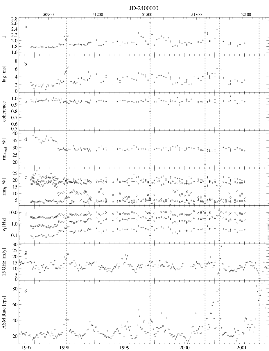
In this section we will discuss the overall behavior of the PSD of Cyg X-1 since 1998. The evolution of the best fit PSD parameters, the X-ray time lag, and the X-ray coherence function, as well as the photon index, $\Gamma$, from the spectral fits, the 15 GHz radio flux, and the RXTE ASM count rate are shown in Fig. 3. Both the radio flux and the ASM count rate have been rebinned to a resolution corresponding to the orbital period of the HDE 226868/Cyg X-1 system ($P_{\text{orb}}=5.599829(16)$ d, see Brocksopp et al. 1999b; LaSala et al. 1998). This rebinning removes the effect of the well known orbital variation of the X-ray and radio flux (Pooley et al. 1999; Brocksopp et al. 1999a; Wen et al. 2001) such that long term changes become more apparent. Due to the rebinning, however, many short flares that are not due to the orbital modulation are smoothed out. We therefore present the radio and ASM data again in Fig. 4 with a higher time resolution, together with the RXTE PCA count rate determined from the monitoring observations. Not unexpectedly, the ASM and PCA rates are well correlated, although their correlation is not perfect due to their different energy bands and the X-ray spectral variability.

3.1 The Two Hard States

The most striking result of our fits is the bimodal behavior of the total rms amplitude (Fig. 3d): Starting in 1998 mid-April, the overall variability of Cyg X-1 on short timescales showed a decrease of $\sim$7%, from an average rms amplitude of 36$\pm$1% to 29$\pm$1%. At the same time, the power law index of the X-ray spectrum slightly softened from $\sim 1.75$ to $\sim 1.85$, the characteristic frequencies of $L_{1}$ through $L_{3}$ shifted to higher values, and the X-ray time lag increased. Furthermore, a larger fraction of observations requires the power law component below $\sim$0.01 Hz. Apart from further “X-ray flares”, which we will describe in Sect. 3.2, Cyg X-1 has remained in this softer and less variable (on short time-scales) X-ray state. Table 3 summarizes the main properties of the PSD before, during, and after the 1998 changes.

The parameters for the X-ray spectrum and timing behavior measured before 1998 May are very similar to the canonical hard state values for this source. Our campaign shows that these values have not been reached since then, i.e., since 1998 May, Cyg X-1 is exhibiting a behavior that is atypical compared to previously observed hard states of this source. In the following we describe these changes in further detail.

The change of the total rms can be mainly attributed to the behavior of $L_{3}$ (Fig. 3e): while the rms values of $L_{1}$ and $L_{2}$ stay roughly constant, $L_{3}$ declines from its pre-May strength of $\sim 17$% to 10$\pm$3%, i.e., almost half of its original strength. Especially during the X-ray flare in 1998 July, $L_{3}$ cannot be detected at all. Since these events, $L_{3}$ has mainly been present at a level between $\sim$5% and $\sim$10% rms, and was sometimes not detected at all. Typical examples for pre- and post-1998 May power spectra are shown in Figs. 2 and 1, respectively. These figures clearly show the decrease in strength of $L_{3}$, especially in the panels where the PSD has been multiplied with frequency.

In addition to this large change in strength, the whole PSD shifts to higher frequencies (Table 3). The two lowest peak frequencies, $\nu_{1}$ and $\nu_{2}$ increase by a factor of $\sim$3 during the change, while $\nu_{3}$ increases by a factor of $\sim$2. This behavior is not mirrored by the peak frequency of $L_{4}$. The sharp drop from about 60 Hz to 40 Hz at the end of P30157 in $\nu_{4}$ is due to the biasing of its value caused by the low frequency cutoff of our data. We note that although the peak frequencies change, their ratios are remarkably constant over the whole campaign – in fact, the 1998 May event is only barely discernible in the evolution of the frequency ratios (Fig. 5).

Figure 6: Normalization of the four broad noise components, $R_{i}$, versus their peak frequencies, $\nu_{i}$. The different plot symbols are attributed to the same components as in Fig. 3.

The nature of the change in the hard state timing behavior can be clearly seen when the variations in the variability amplitudes and peak frequencies are considered together. Fig. 6 shows the dependence of the normalization constant, $R_{i}$, of each broad component on the associated peak frequencies, $\nu_{i}$, for our data. Regions in Fig. 6 where the data point density is higher are due to the hard state behavior before and after 1998 April.

Several interesting features are apparent in Fig. 6. The three lowest frequencies, $\nu_{1}$ through $\nu_{3}$, form a continuum from about $5\,10^{-2}$ Hz to 20 Hz. For all three Lorentzians, the normalization of the Lorentzian correlates with its peak frequency – higher $\nu_{i}$ also imply a lower normalization. Furthermore, in those frequency regions, where several Lorentzians can be found, e.g., around 0.5 Hz for $\nu_{1}$ and $\nu_{2}$, and around 5 Hz for $\nu_{2}$ and $\nu_{3}$, their normalizations seem to be the same. We stress that this is not due to a misidentification of the Lorentzians as these are always clearly distinguishable in the observations presented here. There are two distinct regions of the $R_{i}$-$\nu_{i}$ correlation: below $\sim 3$ Hz, where the figure is dominated by $L_{1}$ and $L_{2}$, and above 3 Hz, where $L_{3}$ dominates. Clearly, $\nu_{3}$ and $R_{3}$ are much more strongly correlated than the parameters for the low frequency Lorentzians. We note that the sharpness of this correlation might in principle have been influenced by the 32 Hz maximum frequency of our 1998 data set. However, the strong $R_{3}$-$\nu_{3}$ correlation is also present when only considering the P40099 and P50110 data. We speculate that these correlations are similar to the effect first seen by Belloni & Hasinger (1990b) in terms of their broken power law analysis of the PSDs of Cyg X-1, where the break frequency of the PSD is correlated with the total source rms variability. In our Lorentzian decomposition, $\nu_{1}$ is roughly equivalent to the break frequency and shows a similar behavior. What is new, and not yet understood, however, is the behavior of $L_{3}$.

Finally, the highest peak frequency component, $L_{4}$ (triangles), is clearly distinct from the lower frequency features and shows a different behavior. Its peak frequency and normalization are comparatively stable. The clustering of the data at 40 and 60 Hz again reflects the fact that $\nu_{4}$ has been systematically over-estimated during P30157. During P40099 and later, however, no systematic changes are seen in $\nu_{4}$, although our data should have been sensitive to such changes.

Figure 7: Correlations a) between the average time lag in the band between 2–4 keV and 8–13 keV and the peak frequencies $\nu_{1}$, $\nu_{2}$, and $\nu_{3}$ of the lower three Lorentzians, b) between the photon index, $\Gamma$, of the X-ray spectrum and $\nu_{1}$ through $\nu_{3}$, and c) between $\Gamma$ and the X-ray time lag. The symbols in panels a and b correspond to those used in Fig. 3.

Figure 8: Peak frequencies of $L_{1}$, $L_{2}$, and $L_{3}$ as determined for the energy band from $\sim 2$–4.6 keV versus the peak frequency for the energy band from 8.4–13.1 keV. The symbols correspond to those used in Fig. 3.

We now discuss the properties of the Lorentzians in terms of other measured quantities (Fig. 7). The distinct behavior of the Lorentzians when plotted against the X-ray photon spectral index, $\Gamma$, and the X-ray time lag gives us further confidence in the individual identifications of the Lorentzians. Both the X-ray time lag and the peak frequencies $\nu_{1}$ through $\nu_{3}$ are clearly correlated with $\Gamma$: softer photon spectra imply a shift of the PSD towards higher frequencies and also higher X-ray time lags (Fig. 7b and c). There is also a clear correlation between the average time lag and the Lorentzian peak frequencies (Fig. 7a). Although a correlation between photon index and frequency has been noted before with more limited data sets (di Matteo & Psaltis 1999; Gilfanov et al. 1999; Revnivtsev et al. 2000; Nowak et al. 2002), this is the first time that a simultaneous correlation with the time lags has been found for Cyg X-1. A similar behavior has been seen in a more limited hard state data set of GX 339$-$4 (Nowak et al. 2002). Recently, a comparative study of the “QPO–$\Gamma$” correlations has been performed for several BHCs with narrow QPOs by Vignarca et al. (2003). While the direct identification of one of our correlations of Fig. 7b with the unified track displayed in their work is not easily possible (different spectral models were used to derive $\Gamma$), the parameter space is comparable. We do not see any turnoff, i.e., no decreasing photon index at high frequencies which seems to be a common feature in some of the sources studied by Vignarca et al. (2003) (mainly GRS 1915$+$105, GRO J1655$-$40, and XTE J1550$-564$). This is consistent with the picture suggested by those authors that the turnoff might be related to a transition between the hard and the very high state, since the latter is not observed in Cyg X-1 (at least not in its canonical form, note, however, that the hard spectral component is generally present also in the soft state).

We note that there is no strong energy dependency of the power spectrum shape during the normal hard state phases. As an example, Fig. 8 shows the correlation between the peak frequency of $L_{1}$, $L_{2}$, and $L_{3}$ for the two energy bands for the 1998 data. To within their error bars, the peak frequencies of $L_{1}$ and $L_{2}$ are identical for these bands. The peak frequency of $L_{3}$ is higher by about 30% in the hard energy band, a trend that continues when analyzing lightcurves in even harder energy bands. This trend is similar to that seen in the Lorentzian decomposition of the PSD of XTE J1650$-$500 (Kalemci et al. 2003).

Figure 9: a–d) Examples of power spectra that deviate significantly from the typical hard state shape as defined by Figs. 1 and 2. The best fit broad noise components are distinguished by their line styles: dashed: $L_{1}$, solid: $L_{2}$ and $L_{3}$, dash-dotted: $L_{4}$. The remaining components and the total best fit are dotted. The observation dates are given in the plot, they are also marked by dotted lines in Figs. 3 and 4.

3.2 Failed State Transitions

In this section we study the behavior of Cyg X-1 during the “flares” apparent in the ASM lightcurve of Fig. 3. During these flares, the rms amplitude decreases, the strength of the power law contribution relative to the Lorentzians increases, and the X-ray spectrum softens. Generally, the X-ray time lag also shows values that are much higher than those seen before and after the flare, and the coherence function drops. PSDs measured during several of these events are shown in Fig. 9. These examples are significantly different from the “standard PSD shape” for the hard state as defined in Figs. 1 and 2.

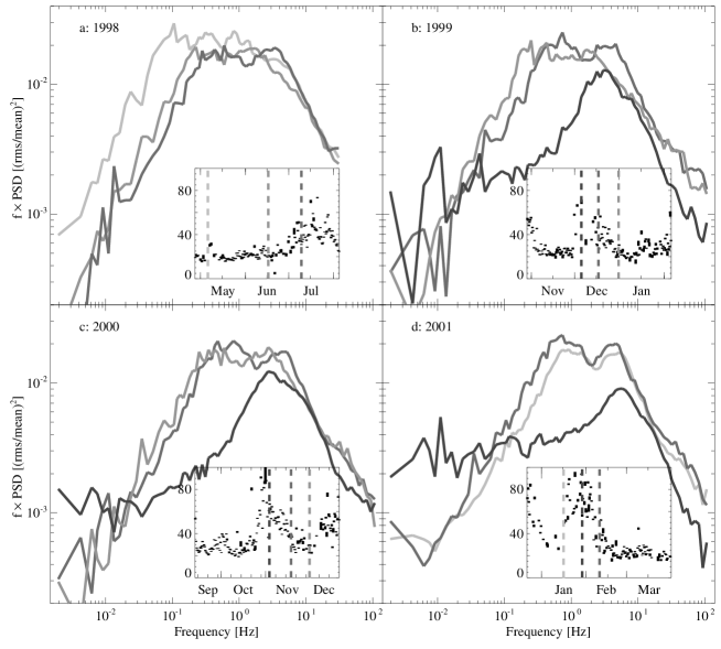
Crucial to the interpretation of these flares is the evolution of the PSD and the other timing quantities over the flares. We will concentrate on the flares best sampled by our monitoring observations. These flares, which were observed in 1998 July, 1999 December, and 2000 November, are identified by dashed lines in Fig. 3. Additional smaller events were also seen, e.g., in 1999 September, in 2000 March, and in 2000 December. For these latter events, however, our observations did not sample the change of the PSD in sufficient detail.

Figure 10: Development of the power spectra near the flaring events seen in the ASM lightcurve. Their location in the ASM lightcurve is indicated in the insets. The panels show the data from a) 1998 July, b) 1999 December, c) 2000 October/November, and d) 2001 January/February.

A typical example for the evolution during the first stage of these flares was seen in 1998 July (Figs. 9 and 10): Here, the characteristic frequencies of the Lorentzians shift to higher frequencies and their relative strength changes. In contrast to the standard PSD, the $L_{3}$ component is weak or missing and the peak frequencies of $L_{1}$ and $L_{2}$ are significantly enhanced. Furthermore, the X-ray time lag in the 3.2–10 Hz band increases (Fig. 3b, see also Pottschmidt et al. 2000). On the resolution of our monitoring, the transition back into the hard state mirrors that of the transition into the flare.

We briefly note that during the 1998 July event there is a change in the energy dependency of the rms variability amplitude (Fig. 11). Before the flare, the rms variability amplitude of $L_{3}$ increased with photon energy, that is the PSD was flatter at higher energy bands as is typical for the hard state (Nowak et al. 1999a). During the flare, when the spectrum was soft, the rms variability amplitude decreased with energy. This is best illustrated in the behavior of $L_{1}$, where the total power in this component before the 1998 July event has a rather small energy dependence (Fig. 11, solid lines), while it is strongly energy dependent during the flare (Fig. 11, dashed lines).

Figure 11: Change of normalization of $L_{1}$ as a function of energy during the first half of 1998. Solid lines: Average of the normalization of $L_{1}$, $R_{1}$, for observations P30157/19 through 28, before the 1998 July failed state transition. Dashed lines: Average of $R_{1}$ for observations P30157/29 through 33, during the 1998 July event.

Figure 12: Evolution of the PSD during the monitoring observations of 2000 November. The line style of the best fit components is the same as that in Fig. 9.

During some of the flares the PSD evolution starts similar to 1998 July but then continues until a strong low-freqency power law dominates the observed rms, instead of the Lorentzians. Typical examples for such a behavior are observations made on 1999 December 05 and on 2000 November 03, at the peak of their respective outbursts (Figs. 10b and c). Of the Lorentzians, $L_{2}$ is strong and $L_{3}$ is clearly present, albeit at the weak levels typical of PSDs observed after 1998 May. On the other hand, $L_{1}$ is barely identifiable. Both observations also have quite large X-ray lags (e.g., $\sim$8 ms for 2000 November) and decreased coherence (e.g., 0.6 on 1999 December 05). The neighboring observations, however, display the characteristic double-peaked PSD similar to 1998 July, coherence close to unity, and lower lags of $\sim$3 ms. The evolution of the Lorentzians through the 2000 November flare is shown in Fig. 12. Both, the PSD shape as well as the X-ray spectral parameters seen here are very similar to earlier observations of Cyg X-1 reported by Belloni et al. (1996). Comparing the timing properties and spectrum of GS~1124$-$683 (Nova Muscae 1991; Ebisawa et al. 1994; Miyamoto et al. 1994) and GX 339$-$4 (Méndez & van der Klis 1997) to those of Cyg X-1, Belloni et al. (1996) found these to be very similar to the “intermediate state” seen in these X-ray transients. In transients, the “intermediate state” is typically seen during transitions between the soft and the hard state, which fits the picture drawn above from our RXTE monitoring.

Based on our observations of increased X-ray time lags during the transitional phases between the 1996 hard and soft state and during the ASM flares, we have previously called the ASM flares “failed state transitions” (Pottschmidt et al. 2000). As outlined above, the behavior of the other timing quantities apart from the X-ray time lags now justifies our use of this term – during the “failed state transitions”, the source changes its behavior compared to the normal hard state, by sometimes even entering the intermediate state, but a full soft state is generally not reached, at least not on the sampling timescale of our RXTE monitoring.

The availability of the different timing quantities for our monitoring observations also allows us to connect the increased X-ray time lag with the observed changes in the power spectrum and the coherence function. As we mentioned above, the X-ray time lag varies strongest in the 3.2–10 Hz band (Pottschmidt et al. 2000). The main contributions to the total rms variability in this frequency range are due to $L_{2}$ and, to a lesser extent, due to $L_{3}$. These two components are also the only broad noise components that are clearly present in the intermediate states of 1999 December 05 and 2000 November 03 power spectra (Fig. 9b and d), as well as during the transition to the soft state in 1996 (Fig. 2 of Pottschmidt et al. 2001; see also Belloni et al. 1996). Since the time lag behavior does not seem to reflect the transient behavior of the $L_{3}$ component, and since the frequency range showing the enhanced lags is more consistent with that of $L_{2}$, we tentatively identify the enhanced time lag during failed state transitions as being mainly due to $L_{2}$. Since the soft state itself shows neither these broad noise components nor enhanced time lags, our identification provides a self-consistent picture.

While most of the ASM flares are indeed “failed state transitions”, there is one flare during the time period covered here, in 2001 January, where the state transition did not fail, but where a soft state was reached for a brief time. The evolution of the PSD shown in Fig. 10d displays again the vanishing of $L_{1}$ and $L_{4}$, with an “intermediate state” PSD observed on 2001 January 29. From the point of view of our monitoring campaign, this behavior would have led us to classify this flare as yet another failed state transition. In addition to our RXTE monitoring, however, further pointed RXTE observations were performed in early 2001, that had a much better sampling than our campaign. The analysis of these data by Cui et al. (2002) shows PSDs that are similar to those seen here, with the exception of the data taken on 2001 January 28. Both the timing and spectral behavior are very similar to the 1996 soft state, leading Cui et al. (2002) to claim a possible short soft state of Cyg X-1.

We note that in addition to the X-ray properties, the radio flux was also peculiar in 2001 January. During the end of 2001 January, the radio flux first dropped to about 30% of its typical value of $\sim$15 mJy, before a radio flare was seen (Figs. 3g and 4). In contrast to 1996, however, Cyg X-1 was always detected in the radio, indicating that the system had not settled into the soft state as it did in 1996. In fact, our monitoring observation of 2001 January 29 shows again the transitional PSD. As in 2001 November (Sect. 3.3), therefore, the switch from the soft state (if it can truly be labeled a soft state) back into the intermediate state occurred within one day.

3.3 The 2002 Soft State

Our RXTE observations performed since 2001 September give further credence to the identification of the presence of an “intermediate state” during the transitions from the hard to the soft state. This time, from 2001 September until 2002 October, was the first time since 1996 that Cyg X-1 exhibited again a full soft state behavior in the X-rays and in the radio emission. A detailed description of this soft state will be the subject of a later publication in this series (Wilms et al. 2003), here we will only briefly summarize the observations of the transition into the soft state during the end of 2001 as far as they are connected with the interpretation of the flares with the “intermediate state” (Sect. 3.2).

Figure 13: RXTE ASM count rate and 15 GHz flux of Cyg X-1 during the fall of 2001. The dashes denote the time of those pointed RXTE observations that were part of our monitoring campaign.

Figure 14: Time lags and PSD for the soft state of 2001 Oct compared with other typical soft state, hard state, and failed state transition data.

During 2001 September, the RXTE-ASM rate rose from its typical 20–30 cps to $\sim$100 cps, with precursor flares in July and August (Fig. 13). Reaching its peak in mid-September, the soft X-ray flux first declined, and was found at a lower but still enhanced ASM level of approximately 60 cps in 2001 December, the end of the time period considered here. However, in contrast to previous flares, this time a clear reduction of the radio emission was also observed, with almost zero flux for about one week in the beginning of October (Fig. 13). After that time the radio emission slowly turned on again, although continued flaring in both the radio and the X-rays was observed. The combination of the strong ASM flux and the missing radio emission is typical for a soft state. As shown in Fig. 14, pointed RXTE observations performed in 2001 October show a clear soft state behavior: comparing PSDs and time lags for the two monitoring observations of 2001 October 20 and 2001 November 3 (dashes in Fig. 13) with typical data from failed state transitions and from the 1996 soft state shows that on 2001 October 20 the PSD had a clear $f^{-1}$ shape, turning over at $\sim$10 Hz, an X-ray time lag comparable with that measured during the standard hard state and an X-ray coherence that was close to unity. The time lag behavior, the unity coherence, and the PSD shape are typical for the soft state (Cui et al. 1997; Pottschmidt et al. 2000). The X-ray spectrum of the 2001 October 20 PCA observation in the 3–20 keV range can be very well described by the empirical soft state spectrum of Cui et al. (1997), i.e., the sum of a black body and a broken power law. The broken power law has a photon index of $\Gamma_{1}=2.78\pm 0.03$ below, and $\Gamma_{2}=2.10\pm 0.02$ above the break energy of $E_{\text{b}}=11.1\pm 0.1$ keV ($\chi^{2}=27.5$ for 31 degrees of freedom, assuming an energy independent systematic uncertainty of 0.3%, a reasonable value for the current calibration of the PCA). The temperature of the black body is measured to $kT_{\text{BB}}=0.36\pm 0.03$ keV. The black body contributes 20% to the total 2–10 keV flux of $3.6\times 10^{-8}\,\text{erg}\,\text{cm}^{-2}\,\text{s}$. These spectral parameters are similar to those of the 1996 soft state (Cui et al. 1997), although the observed 2–10 keV flux is a factor $\sim$2 higher. We note that the 2001 October 20 data require an additional and very broad iron line at 6.4 keV (equivalent width $\sim 440$ eV with a Gaussian width $\sigma=0.9\pm 0.1$ keV) that had not been seen in 1996.

On 2001 October 22, RXTE performed a second observation close to this soft state observation. Here, the PSD slightly deviated from the soft state PSD, while the X-ray spectrum was still well described by the empirical soft state model. Shortly after this, during the next monitoring observation on 2001 November 3, the PSD showed an “intermediate state” shape similar to that during the failed state transitions of 1999 November and 2000 December discussed above, i.e., with the $L_{1}$ component missing and an increased power law component. Also pointing towards a transitional behavior are the increased time lag and the reduced X-ray coherence. Both the PSD and the X-ray time lag are similar to the behavior measured on 2000 November 03, one year before the 2001 soft state (see Fig. 14). The X-ray spectrum is much harder and can be well described by the hard state spectral model.

We conclude that in 2001 October and November, Cyg X-1 was switching back and forth between the “classic” soft state and the “intermediate state”. These changes from the soft state to the transitional behavior happened very quickly, within a few days at most. Furthermore, the very similar behavior of the source during the failed state transitions and the 2001 October transition into the soft state provides clear evidence that the ASM flares seen since 1996 are indeed “failed state transitions”, as opposed to being brief “soft states”. As we will show in a later paper (Wilms et al. 2003), after that episode Cyg X-1 settled into a soft state until the end of 2002.

3.4 Narrow Lorentzians

In the previous sections we have described the overall evolution of the four broad Lorentzians, which are responsible for most of the variability observed in Cyg X-1. Here we finish our discussion by concentrating on the additional narrow Lorentzians, $L_{\text{add},1}$ through $L_{\text{add},3}$, which were needed in about 65% of all observations to completely describe the observed power spectra (Sect. 2.3). As these components are always rather narrow, with $Q\gg 2$, we will follow the conventions outlined, e.g., by Belloni et al. (2002) and call these components QPOs. As already mentioned in Sect. 2.3, these QPOs fall into two categories: rather narrow and clearly visible QPOs, $L_{\text{add},1}$ and $L_{\text{add},2}$, with frequencies above roughly 1 Hz, and a broader structure, $L_{\text{add},3}$, at frequencies below 0.2 Hz.

Figure 15: a Number of detected thinner Lorentzian components as a function of $\nu_{\text{add}}/\nu_{1}$ and b $\nu_{\text{add}}/\nu_{2}$. The dashed lines represent the same distribution for QPOs with $Q\geq 50$ only. The dotted line in panel a corresponds to a frequency ratio of 2; in panel b, dotted lines designate frequency ratios of 1:2 and 1:4 with respect to $\nu_{2}$.

Our emphasis on modeling the broad Lorentzians led us to logarithmically rebin the measured PSDs, to the extent that a determination of the parameters of the narrow features was not always possible (see footnote 3). For example, the logarithmic rebinning of the PSDs means that the QPO was concentrated in only a few frequency bins such that its $Q$-value could not be determined. $Q$-factors larger than 50 in Table 2 generally are an indication that these QPOs are concentrated in one frequency bin. The majority of the remaining $Q$-factors cluster between $\sim$2 and $\sim$15, i.e., these QPOs are somewhat broader structures. Due to these limitations in our modeling, we can not quote formal uncertainties for the fit parameters of the QPOs. We will concentrate, therefore, in the following on the frequency behavior of the QPOs, keeping in mind the above problems with the detection and quantification of the QPO features. For consistency with the description of the broad Lorentzians, we will continue to use the peak frequency to characterize the frequency of the QPOs. Due to the large $Q$-values involved, the peak frequency is usually very close to the center frequency of the Lorentzian used to model the QPO.

Turning first to the two narrow QPOs, Fig. 15 shows the distribution of the ratio between the peak frequencies of all narrow Lorentzians to those of $L_{1}$ and $L_{2}$. Note that the majority of these additional PSD components are found between $L_{1}$ and $L_{2}$. There are a few observations in which a QPO is present below the peak frequency of $L_{1}$, while no additional components were required above $L_{2}$. As is clearly shown in Fig. 15a, an appreciable fraction of the QPOs are found at the first harmonic of the peak frequency of the $L_{1}$ component, $\nu_{1}$ ($\sim 20$% of all detected QPOs have peak frequencies in the range $1.8\leq\nu_{\text{add}}/\nu_{1}\leq 2.2$). This enhanced fraction of QPOs at $2\nu_{1}$ suggests a relationship with the broad Lorentzian $L_{1}$. Taken at face value, one might interpret the QPOs in this frequency range as overtones of $L_{1}$, and indeed $L_{1}$ often shows a more complex structure which is modeled away by adding a Lorentzian to the model. We note that such a presence of possibly harmonically related components is not unexpected as it was seen before by Nowak (2000) in his treatment of the PSDs of Cyg X-1 and GX 339$-$4.

We caution, however, that the “overtone” interpretation of this substructure is not the only interpretation. Since $L_{1}$ is broad, one might expect its overtones to be broad as well, and this is not the case: the narrow QPOs with $Q\geq 50$, i.e., those QPOs which are only present in one frequency bin of our rebinned PSDs, have a distribution which is similar to that of QPOs with $Q<50$ (Fig. 15a, dashed lines). Furthermore, since for the peak frequencies of $L_{1}$ and $L_{2}$, $\nu_{2}/\nu_{1}\sim 8$ (Table 3), we have $2\nu_{1}\sim\nu_{2}/4$, such that these QPOs could also be subharmonics of $L_{2}$. We conclude, therefore, that the frequency distribution of the QPOs is indicative of a relationship between at least part of these components and the broad Lorentzians, but that the quality of the current data is not good enough to distinguish between the different interpretations. This is especially true given that the Lorentzian shape assumed for $L_{1}$ through $L_{4}$ might only be an approximation to the real shape of the broad components that apparently comprise the PSD.

Finally, we turn to the broad additional Lorentzian present at frequencies $<0.2$ Hz, $L_{\text{add},3}$. In about half of the 17 observations in which this component was present, an additional power law component was also required in the description of the data. Our data indicate a very loose correlation between the $Q$-value of $L_{\text{add},3}$ and its peak frequency. As shown in the previous sections, PSDs containing a power law component are one indicator of (failed) state transitions. The presence of $L_{\text{add},3}$ in these PSDs thus indicates that the PSD during the failed state transitions is slightly more complicated than the simple sum of a power law and the four broad Lorentzians and that the low frequency PSD is more structured during these events (see, e.g., Miyamoto et al. 1994 and Belloni et al. 1996). Finally, we note that we have not found statistically significant correlations between the peak frequency of $L_{\text{add},3}$ and that of $L_{1}$ through $L_{4}$ or the narrow QPOs . The quality of our PSDs at low frequencies is not good enough, however, to allow a more detailed analysis.

4 Discussion and Conclusion

4.1 Summary

The rapid high energy variability of galactic black holes is still not understood. The behavior of the PSD and the time lags during our campaign, however, gives some clue as to its origin.

The most important result of this paper is that the shape of the PSD during the hard state and during the intermediate state can be productively interpreted with the decomposition of the PSD into the four broad peaked components, which we model as Lorentzians, and one power law. In contrast to earlier analyses, we were able to show that the decomposition holds for a very wide range of source parameters, even though the contributions of the power law and the Lorentzians are very different in the different states. Our result therefore adds further weight to the claim that the four broad Lorentzians are not just a convenient description of the PSD (merely more successful than the approximation of a broken power law), but that instead the broad components are the fundamental building blocks of the PSD of Cyg X-1 and thus possibly also of the PSDs of other black hole candidates. We emphasize that a statistically significant discrimination between different shapes of the Lorentzians is not possible with the available data (see Sects. 2.3 and 3.4, and Belloni et al. 2002), however, our study shows that any alternative building blocks for the PSD must at least be similar in shape to the broad components revealed by our analysis.

Furthermore, there are two fundamental results from our campaign on the long term variability of the source. The first result is that the change of the general long term behavior of Cyg X-1 from a “quiet hard state” to a “flaring hard state”, with frequent intermittent failed state transitions after 1998 May, coincided with a change in the PSD shape and amplitude. After 1998 May, $L_{3}$ was clearly much weaker than before. At the same time, the whole PSD shifted towards higher frequencies in a way that preserved the ratio between the peak frequencies, a larger fraction of PSDs showed low frequency noise, the X-ray lag increased, and the average X-ray spectrum softened. The tendency for a softening of BHC spectra to correlate with a frequency shift of characteristic features of the PSD has also been seen in other sources (di Matteo & Psaltis 1999; Gilfanov et al. 1999; Revnivtsev et al. 2000; Kalemci et al. 2001; Nowak et al. 2002), and thus might be considered an intrinsic feature of all BHCs.

The second result of our campaign concerns the change in the PSD shape during the X-ray flares. We interpret these flares as transitions from the hard state via the intermediate state into the soft state. Most of these transitions “failed”, i.e., the transition stopped before the soft state was reached. That the “failed transitions” are caused by the same physical mechanism as the normal transitions into the soft state was shown by the two instances during the campaign where a brief soft state was observed (Sect. 3.2). In these cases, before the soft state was reached and after it was left again, the source behavior was indistinguishable from the behavior during the “failed transitions”.

On the way into the intermediate state, $L_{2}$ and $L_{3}$ almost remained constant, while $L_{1}$ – and, to a lower significance, also $L_{4}$ – became remarkably weaker. At the same time, the X-ray spectrum softened and the whole PSD shifted to higher frequencies. Furthermore, the X-ray time lag increases in the 3.2–10 Hz frequency band during the transitions and the coherence function decreases. This is the frequency band where the PSD is dominated by the $L_{2}$ and, to a lesser extent, the $L_{3}$ components. In those cases where the soft state was reached, the X-ray lag spectrum and the coherence function during the soft state were found to be very similar to that of the normal hard state, while the PSD, in contrast to the typical hard state, showed its characteristic $f^{-1}$ shape with a cut-off at $\sim$10 Hz. During the soft state, no radio emission was detected. Such a detailed study of the hard state and transitions has to date only been possible for Cyg X-1. We note, however, that observations with a sparser coverage show similar behavior for GX 339$-$4 (Nowak et al. 2002) and for XTE~J1650$-$50 (Kalemci et al. 2003).

Figure 16:  Correlations between the peak frequencies of the broad noise components, $L_{1}$–$L_{4}$ and the frequency correlations discussed by Psaltis et al. (1999, solid lines are $\nu_{y}=42\,\text{Hz}\,(\nu_{x}/500\,\text{Hz})^{0.95\pm 0.16}$). a) $\nu_{1}$ versus $\nu_{2}$, b) $\nu_{2}$ versus $\nu_{3}$, c) $\nu_{1}$ versus $\nu_{3}$. d) $\nu_{1}$ (crosses), $\nu_{2}$ (diamonds), and $\nu_{3}$ (circles) versus the highest peak frequency, $\nu_{4}$. Only data taken in P40099 and P50110 are shown in panel d to avoid biasing due to the 32 Hz frequency cutoff in the P30157 data.

4.2 Relationship between Neutron Star and Black Hole Sources

Apart from the analysis of Nowak (2000), Lorentzian modeling has also been used for describing the power spectra of neutron star sources. A recent summary of Lorentzian fits to data from neutron stars and black holes has been recently published by Belloni et al. (2002). These authors base their work on their analysis of RXTE observations of six neutron star sources (1E~1724$-$3045, SLX~1735$-$269, GS~1826$-$24, XTE~J1118$+$480, Cir X-1, and GX~17$+$2), as well as on published results from the black holes Cyg X-1, GX 339$-$4 (Nowak et al. 2002), and XTE~J1550$-$05 (Homan et al. 2001), and the neutron star sources 4U~1915$-$05 (Boirin et al. 2000) and 4U~1728$-$34 (Di Salvo et al. 2001). Furthermore, van Straaten et al. (2002) have recently published an extensive analysis of data from 4U~0614$+$09 and 4U~1728$-$34.

Belloni et al. (2002) and van Straaten et al. (2002) find that one to six Lorentzians are required to obtain a good description of the PSDs of these sources. A slight complication when comparing these results to ours is that van Straaten et al. (2002) and Belloni et al. (2002) mainly use zero frequency centered Lorentzians, i.e., shot-noise profiles, and not Lorentzians with non-zero center frequencies. As we describe in Sect. 2.3, our choice appears to result in a slightly lower $\chi^{2}$ (but note the discussion in Sect. 2 of Belloni et al. 2002). Despite the different fit functions, however, the behavior of the maximum frequencies in both cases is still comparable. In terms of ascending $\nu$, van Straaten et al. (2002) call $L_{1}$ and $L_{2}$ the band-limited noise and zero-centered Lorentzian, $L_{3}$ the low-frequency Lorentzian, and $L_{4}$ the hectohertz Lorentzian. In the notation of Belloni et al. (2002), $L_{1}$ corresponds to $L_{\text{b}}$ as this is the Lorentzian describing the break frequency of the PSD. The Lorentzians $L_{3}$ and $L_{4}$, which describe the lower and upper characteristic frequencies in the tail of the PSD, are called $L_{\text{l}}$ and $L_{\text{u}}$. In many neutron star PSDs the $L_{2}$ component has a rather large $Q$, therefore, Belloni et al. (2002) identify $L_{2}$ with the low frequency QPO, $L_{\text{LF}}$.

Note that the for all sources the “correct” identification of these components is difficult. For example, $L_{1}$ and $L_{2}$ are not present together in all data sets such that one might misinterpret the band limited noise (to stay in the terminology of van Straaten et al. 2002) as the zero-centered Lorentzian. Similar problems also apply for Cyg X-1: had the spacing of our observations during the (failed) state transitions been coarser, we would not have been able to correctly identify the Lorentzians during the state transitions.

At higher frequencies, additional narrow Lorentzians are required to describe the kilohertz Lorentzians in neutron star sources, however, their connection to the PSDs of BHCs is less clear. Nowak (2000) argue tentatively that $L_{4}$ could be identified with the upper kilohertz QPO, however, the observed behavior of this component by van Straaten et al. (2002) casts some doubt on this interpretation: while neutron star kHz QPOs are varying in frequency, $L_{4}$ clearly does not (e.g., Fig. 6). On the other hand, van Straaten et al. (2002) point out that there is a broad feature around 100 Hz, the “100 Hz bump”, which is constant in frequency and therefore a more probable counterpart to $L_{4}$.

There are two main correlations among frequency components that have been claimed for neutron star and black hole sources (see Belloni et al. 2002 for a recent summary). Wijnands & van der Klis (1999) have pointed out a correlation between the PSD break frequency and the low frequency QPO of X-ray binaries. These two frequencies might be related to $\nu_{1}$ and $\nu_{2}$ in our classification scheme. Psaltis et al. (1999) have pointed out a correlation between the low frequency QPO and the lower frequency kHz QPO, i.e., frequencies that could be identified with $\nu_{2}$ and $\nu_{3}$ in our scheme. The latter correlation especially relies on identifying these features in multiple sources. The origin of these correlations is unknown.

In Fig. 16 we plot various combinations of one frequency versus another, and show that with the exception of $\nu_{4}$ all frequency combinations show some sort of correlation (this is just a consequence of the constancy of the frequency ratios shown in Fig. 5). Similar correlations for several sources are also shown by Belloni et al. (2002, Figs. 11 and 12), who point out that – while all different sources seem to show correlations between individual Lorentzians – these do not seem to completely agree from source to source. Given the above two correlations, the one that fits our data best is the correlation described by Psaltis et al. (1999), albeit applied to the $\nu_{1}$ versus $\nu_{2}$ correlation. We note, however, that in this particular range of frequencies, the $\nu_{1}$ versus $\nu_{2}$ correlation cited by Wijnands & van der Klis (1999) is numerically not very different than the $\nu_{2}$-$\nu_{3}$ correlation of Psaltis et al. (1999). Likewise, the $\nu_{2}$-$\nu_{3}$ data presented here are marginally consistent with the correlation discussed by Psaltis et al. (1999). Although the individual components discussed here span more than a decade in frequency, this is not large enough a range to identify unambiguously given features with the three decade wide correlations hypothesized and discussed by Psaltis et al. (1999). Still, correlations among the frequency components clearly do exist, and point to possible physical scenarios, as we further discuss below.

4.3 A Possible Physical Scenario

We now discuss the empirical evidence from our campaign in terms of more physical models for the accretion process in a black hole system. The hard state X-ray spectrum is thought to be caused, at least in part, by soft photons from the accretion disk which are Compton upscattered in a hot electron gas (Sunyaev & Trümper 1979; Dove et al. 1998; Poutanen & Svensson 1999, and references therein). In this picture, state transitions are caused by the disappearance of this Comptonizing medium. The cause for this disappearance is unknown, however, due to the luminosity difference between the hard and the soft state, many workers have assumed that the Compton corona is produced by some physical process which can work only at mass accretion rates below a certain threshold rate such as the magnetorotational instability (Balbus & Hawley 1991), advection (Esin et al. 1997), or some kind of coronal outflow (Merloni & Fabian 2002; Blandford & Begelman 1999, and references therein), while others have claimed the presence of an up to now unknown additional parameter which triggers the state transitions (Homan et al. 2001). A similar picture of changing coronal properties should also hold true within the hard state itself – although the Compton corona exists throughout the hard state, phases where a different X-ray spectrum and PSD are observed might well correspond to different coronal geometries (Nayakshin et al. 2000; Liu et al. 1999; Esin et al. 1997; Smith et al. 2002, e.g.,). Such a change in the coronal configuration could explain the reduction of the $L_{3}$ component after 1998 May, as is also evidenced by an overall softening of the spectrum since that time.

We note that for Cyg X-1 the luminosity difference between the hard and soft state is rather small ($\sim$35%; Zhang et al. 1997a). Furthermore, a power law component is always seen during the soft state. This suggests that the soft state in Cyg X-1 might not be a “normal” soft state as that seen in other black holes, but rather closer to the very high state than the canonical soft state is. Furthermore, there are cases where the soft state has not a higher luminosity but a lower luminosity than the hard state. For GRS~1758$-$258, an intermediate state has even been observed at a higher luminosity than the hard state, while the soft state appears to be at a much lower luminosity (Smith et al. 2001). A possible explanation for these deviations from the canonical picture of the soft state having a much higher luminosity than the hard state might be an hysteresis effect (Miyamoto et al. 1995), however, we note that regardless of the physical cause for deviations the observational evidence still points towards changes in the accretion disk geometry.

That the accretion disk geometry changed around 1998 May might also be the cause for the shift of the peak frequencies towards higher frequencies observed during that time. Even in prior analyses where PSDs of BHC have been described in terms of power law fits and “shot noise models” (Lochner et al. 1991, and references therein), it has been presumed that the characteristic frequencies can be attributed to time scales of the accretion disk. Churazov et al. (2001) have argued that PSD “breaks” are related to the size scale at which the accretion flow transits from a thin disk into a geometrically thick, hot inner corona. Di Matteo & Psaltis (1999) have argued that the dynamic range over which such a transition varies is somewhat limited since the observed frequencies themselves, although variable and correlated with spectral hardness, only span a limited range. Since flow frequencies scale as $\delta\nu/\nu\sim(H/R)^{2}$ (e.g., di Matteo & Psaltis 1999, and references therein), if the Lorentzians are associated with resonant effects within the accretion disk, they must originate from a region that is geometrically thicker than the thin accretion disk, i.e., a comparably extended region such as the accretion disk corona.

A simplified analysis of the characteristic frequencies of such a transition region has been presented by Psaltis & Norman (2001). These authors note that if the outer disk acts as a “noise source”, the transition region acts as a “filter”, and the inner corona acts as a “response” which processes the filtered noise into observable X-ray variability, then one expects to observe a number of quasi-periodic features. These features would be related to radial, vertical, acoustic, rotational, etc., oscillations of the transition region. Many of these frequencies would be expected to scale as $R_{\text{T}}^{-3/2}$, where $R_{\text{T}}$ is the transition region radius. More recently, Nowak et al. (2002) have shown that such a scaling might exist for hard state observations of GX 339$-$4. Specifically, they show that in “sphere and disk” coronal models, the “coronal compactness” – where higher compactness, $\ell_{\text{c}}$, means harder spectra – scales as $\ell_{\text{c}}\propto R_{\text{T}}$. Furthermore, the characteristic PSD frequencies, measured in a manner similar to that used to describe the Cyg X-1 PSDs presented here, scale as $\ell_{\text{c}}^{-3/2}$. Both Cyg X-1 and GX 339$-$4, in their hard states, show that spectral softening is correlated with higher PSD frequencies, although we have yet to characterize the Cyg X-1 spectra in terms of the coronal models presented by Nowak et al. (2002). Such an analysis is currently underway (Gleissner et al. 2003).

Further hints towards attributing at least some of the Lorentzians to the Compton corona come from the PSD behavior during the transitions into the intermediate or the soft state. We hypothesize that the variability causing $L_{1}$ and possible $L_{4}$ is also associated with the accretion disk corona, since these components – like the corona – appear to vanish during the transition. Since $L_{2}$ and $L_{3}$ remain present in the 3.2–10 Hz band, we are tempted to attribute the increased X-ray time lag in this frequency band to these components. As discussed by Nowak (2000), the overall measured time lag may in reality be a composite of time lags inherent to each individual PSD component. Whereas the composite time lag might be fairly small, the time lags associated with the individual PSD components might be somewhat larger (specifically, see Fig. 5 of Nowak 2000). The fairly long intrinsic time lags of these individual PSD components would only be revealed in the absence of the other PSD components. Such a picture might explain the larger X-ray time lag during state transitions: Here, the $L_{2}$ and $L_{3}$ components, which sit in the 3.2–10 Hz band, contribute a larger relative fraction of the total source variability. If their intrinsic lag is larger, a larger lag would be observable during state transitions when the contribution of $L_{1}$ and $L_{4}$ is reduced. We note that such a picture of a “composite X-ray time lag” is somewhat suggested by the observational shape of the time lag spectrum, where “jumps” between different frequency bands of roughly constant time lag seem to correspond to the overlap regions of the broad Lorentzians (Nowak et al. 1999b; Poutanen 2002; Pottschmidt et al. 2000).

While the origin of the time lag is not yet understood, it is possible that the time lag is somehow related to a characteristic length scale of the medium which produces the observed photons. If this is true, then the larger lags during state transitions may be showing that some part of the source geometry changes and becomes larger during the transitions. It is important to note that although there is no radio emission during the soft state, there does seem to be a slight increase of the radio flux at least during some of successful transitions into and out of the soft state (Corbel et al. 2000; Zhang et al. 1997b). Furthermore, intermittent, rapid radio flaring activity also seems to be associated with the (failed) transitions (Pooley, priv. comm.).

In general, we see that the time lags are correlated with the PSD frequencies and correlated with the photon index, $\Gamma$ (Fig. 7a in Sect. 3). For GX 339$-$4, spectral fits with the coronal model of Coppi (1999) – where a spherical corona with seed photons distributed throughout it according to the diffusion equation is modeled – suggest an increasing radius with a softening spectrum (Nowak et al. 2002), consistent with a geometric interpretation of increased time lags. Nowak et al. (2002) therefore argued for a jet-like model for the hard state of GX 339$-$4 where the radius of the base of the jet followed the radius-frequency correlations suggested by the “sphere and disk” coronal model (i.e., smaller base radius yielding softer spectra), while the vertical extent of the corona/jet followed the correlations suggested by the Coppi coronal model (i.e., more vertically extended coronae yielding softer spectra). Thus, frequencies might be generated at the base of the jet, while time lags could be generated via propagation along the jet. Given the similar, but much more detailed, correlations observed here in Cyg X-1 it is tempting to ascribe the same type of model to these data. Whether the analogy to GX 339$-$4 holds in detail will depend upon the results of detailed coronal model fits (Gleissner et al. 2003).

Along these lines, based mainly on observations of microquasars, Fender (2001) and Fender et al. (1999) have recently attempted to unify the radio and X-ray observations into a geometrical picture of the region surrounding the central black hole. We have previously suggested that the enhanced X-ray lags during the “flares” observed in Cyg X-1 seem to add credibility to this picture (Pottschmidt et al. 2001). During the normal hard state, there is a weak outflow of material from the region surrounding the black hole. This outflow is responsible for producing the observed synchrotron radio emission. We think it likely that the base of this outflow coincides with the accretion disk “corona” that produces the hard state X-ray spectrum and is, given the results above, also responsible for part of the observed X-ray variability. During the “flares”, part of the corona gets ejected. Thus the mass of the radio outflow is temporarily enhanced, increasing the radio luminosity. As the corona is disturbed, whatever resonant mechanism producing the $L_{1}$ and possibly also the $L_{4}$ variability will be disturbed, resulting in a decrease of its contribution to the total rms variability. Furthermore, if this “corona” is “stretched” because of the ejection, it seems likely that a temporary increase in the X-ray lags should be associated with the outflow as the characteristic length scales increase. During the soft state, the corona has fully vanished such that no radio outflow is observed and the X-ray spectrum is soft. If $L_{2}$ and $L_{3}$ are produced at the corona-disk interface, they also vanish.

This very rough picture leaves many detailed questions open, such as the explanation for the strong domination of the $f^{-1}$ power law during the soft state, its cutoff frequency, the generation of the intrinsic lag of the Lorentzians, or the physical mechanisms responsible for the PSD itself. However, we believe that monitoring campaigns such as this one, that are able to assess the long term, systematic changes in accreting systems, will continue to constrain the parameters of the observed physical systems and will enable us to switch from describing the “accretion disk weather” towards understanding the “accretion disk climate”. Equally importantly, X-ray astronomy is entering a phase of high spectral resolution observations with such instruments as Chandra and XMM-Newton. The nature of these instruments does not allow detailed and intensive monitoring campaigns such as this one. However, given the continued operation of the RXTE-ASM and judicious use of simultaneous pointed RXTE observations, campaigns such as this will allow these individual high resolution observations to be placed within their proper ‘global’ context.