Is the Universe Inflating? Dark Energy and the Future of the Universe

Abstract

We consider the fate of the observable universe in the light of the discovery of a dark energy component to the cosmic energy budget. We extend results for a cosmological constant to a general dark energy component and examine the constraints on phenomena that may prevent the eternal acceleration of our patch of the universe. We find that the period of accelerated cosmic expansion has not lasted long enough for observations to confirm that we are undergoing inflation; such an observation will be possible when the dark energy density has risen to between 90% and 95% of the critical. The best we can do is make cosmological observations in order to verify the continued presence of dark energy to some high redshift. Having done that, the only possibility that could spoil the conclusion that we are inflating would be the existence of a disturbance (the surface of a true vacuum bubble, for example) that is moving toward us with sufficiently high velocity, but is too far away to be currently observable. Such a disturbance would have to move toward us with speed greater than about $0.8c$ in order to spoil the late-time inflation of our patch of the universe and yet avoid being detectable.

I Introduction

There is now considerable evidence that the universe is dominated by a peculiar energy component with negative pressure. This component, called dark energy, leads to the acceleration of the universe and explains why type Ia supernovae of intermediate redshift are observed to be dimmer than they would be in a matter-only universe Riess:1998cb ; Perlmutter:1998np . Dark energy also obviates the apparent discrepancy between large-scale structure measurements, which indicate that matter comprises around 30% of the critical energy density, and cosmic microwave background measurements, which show that the total energy density is very nearly equal to critical. The energy density of this mysterious component, $X$, relative to the critical density is $\Omega_{X}\sim 0.7$ and the equation of state is $-1\leq w\equiv p_{X}/\rho_{X}\leq-0.6$ Perlmutter:1999jt ; Wang:1999fa .

This important discovery raises some interesting and fundamental issues. Of particular interest to us is the possibility that the universe may be entering a stage of inflation Guth:1980zm ; Linde:1981mu ; Albrecht:1982wi , similar to that thought to have occurred in the early universe. If this is the case, we would like to know when the universe started or will start to inflate, when we will be able to observe this inflation, and what observational constraints, if any, exist that could reveal, even in principle, whether the inflationary period will be prolonged or even eternal. To address these questions, we are motivated by the exciting prospects for constraining dark energy using cosmological probes. Type Ia supernovae (SNe Ia) have been the most effective and direct probes to date, and give strong evidence for the existence of the negative-pressure component Riess:1998cb ; Perlmutter:1998np . Number counts of galaxies newman and galaxy clusters holder are also very promising techniques, which are sensitive to the growth of density perturbations. While weak gravitational lensing WL and large-scale structure surveys GDM are mostly sensitive to the matter component, and the cosmic microwave background (CMB) primarily probes the total energy density, all three of these provide crucial complementary information; namely the fraction of the total energy density in matter $\Omega_{M}$ and the total energy density $\Omega_{TOT}$ (both in units of the critical density). With the proposed wide-field telescopes, such as the Large-aperture Synoptic Survey Telescope (LSST) on the ground, and the Supernova Acceleration Probe (SNAP) in space, the next decade may offer an order-of-magnitude better constraints on the properties of dark energy.

To address the observability of the fate of the universe, Starkman et al. Starkman:1999pg (heretofore STV) have used the concept of the minimal anti-trapped surface (MAS). The MAS is a sphere, centered on the observer, on which the velocity of comoving objects is the speed of light $c$. In a Friedmann-Robertson-Walker (FRW) cosmology, the radius of the MAS at any given conformal time $\eta_{e}$ is the Hubble radius at that time $H(\eta_{e})^{-1}$. For sources inside our MAS, photons emitted directly at us get nearer with time, while all photons emitted by sources outside the MAS are initially receding from us because of the superluminal recession of the source. If the MAS is expanding (in comoving terms), then the retreating photons will eventually stop retreating and reach the observer – the source will come into view. If the MAS is contracting, many of the photons will never reach us. The authors then argue that comoving contraction of the MAS can be identified with inflation.

The work of STV builds on earlier work of Vachaspati and Trodden Vachaspati:1998dy , who have shown that in a FRW cosmology at conformal time $\eta_{e}$, the necessary and sufficient condition for the contraction of the MAS is that a region of size $H^{-1}(\eta_{e})$, the radius of the MAS, be vacuum dominated. Assuming a flat universe with vacuum energy relative to critical of $\Omega_{\Lambda}=0.8$, STV compute the redshift at which we can observe the MAS to be $z_{MAS}\approx 1.8$. Since the comoving radius of the MAS is equal to the comoving Hubble radius, the condition for the onset of inflation is particularly simple

$$\frac{dH_{\rm comov}^{-1}}{d\eta}=0\ .$$ (1)

STV then conclude that in a flat universe the MAS is directly observable only if $\Omega_{\Lambda}>0.96$, and so, for the currently favored value of $\Omega_{\Lambda}$, this is not possible.

Subsequently several other paper on essentially the same topic have appeared, and we briefly comment on them here. Avelino et al. Avelino:2000ix address the same problem as STV, but replace the criterion for inflation used by STV (i.e., the contraction of the MAS) by the condition that inflation arises when the energy-momentum tensor is vacuum-energy dominated out to a redshift $z=z_{*}$, where the distance to $z_{*}$ is equal to the distance to the event horizon. With this definition, higher $\Omega_{\Lambda}$ implies smaller $z_{*}$, which the authors consider a more reasonable result than the one from STV (in which higher $\Omega_{\Lambda}$ implies higher $z_{MAS}$.) Gudmundsson and Björnsson  Gudmundsson:2001gd introduce the concept of a $\Lambda$-sphere, which they define as the surface within which the vacuum energy dominates and is located at the redshift of the onset of acceleration of the universe. In this work we shall retain the criterion for inflation used by STV, defined by contraction of the MAS. This definition is simple, mathematically precise and intuitively clear and corresponds with the fundamental causal notion of inflation – that in inflation objects are leaving apparent causal contact.

In this paper we extend the analysis of STV in several ways. First of all, in Sec. II we generalize all results from a pure cosmological constant to a general dark energy component described by its fractional density $\Omega_{X}$ and redshift-dependent equation of state ratio $w(z)$. Indeed, although the vacuum energy considered in STV is in many ways the simplest dark-energy candidate, there are a number of other candidates, some of which have been thoroughly explored (e.g. quintessence Ratra:1987rm ; Caldwell:1997ii , or k-essence Armendariz-Picon:2000dh ; Armendariz-Picon:2000ah ). These alternatives can have complex dynamics and lead to observationally distinct cosmic evolutions. In Sec. III we use a toy model to investigate in depth some possible scenarios. Finally, in Sec. IV we discuss in detail what cosmological observations can and cannot tell us about the fate of the universe. Throughout, we assume a flat universe as suggested by recent CMB anisotropy results Netterfield:2001yq ; Pryke:2001yz ; max ; wang . The fiducial model we use is $\Omega_{X}=1-\Omega_{M}=0.7$ and $w(z)=-1$, which corresponds to the current concordance model turner_scripta .

Finally, we make two additional assumptions. First, we assume the validity of the weak energy condition (that is, $w(z)\geq-1$), which is required in order to use the results of Vachaspati and Trodden regarding the MAS Vachaspati:1998dy . Second, we assume that the universe is homogeneous on the current horizon scales (i.e., on scale $\sim H_{0}^{-1}$). Besides being confirmed to a high accuracy by observations, the homogeneity assumption is crucial for our arguments; it follows that the energy content of our patch of the universe is a function of time only (obtained through $\Omega_{M}(z)$ and $\Omega_{X}(z)$) and not space.

II A Generalized condition for inflation

Let us see which dark energy models satisfy the condition (1) on the turnaround of the MAS, and at what redshift.

The energy density in the dark component evolves as

$$\rho_{X}(z)=\Omega_{X}\rho_{crit}\exp\left(3\int_{0}^{z}(1+w(z^{\prime}))d\ln(1+z^{\prime})\right)\ .$$ (2)

The condition for the turnaround of the MAS then simplifies to

$$\rho_{M}(z)+[1+3w(z)]\rho_{X}(z)=0,$$ (3)

or, using the fact that $\Omega_{X}(z)\equiv\rho_{X}(z)/\rho_{crit}(z)$,

$$Q(z)\equiv 1+3w(z)\Omega_{X}(z)=0\ .$$ (4)

Since $dH_{comov}^{-1}/d\eta=0$ is equivalent to $\ddot{a}/a=0$ in an FRW universe, this is precisely the same as the condition that the universe be accelerating. Here $a(t)$ is the cosmic scale factor and a dot denotes a derivative with respect to physical time $t$.

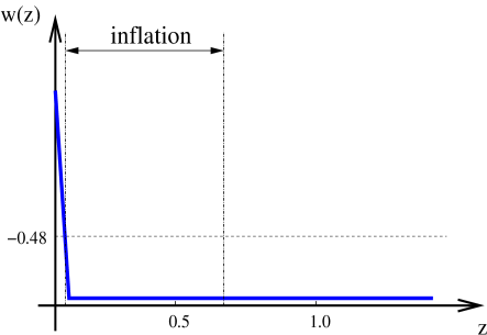
Figure 1: Abrupt variations in $w(z)$ may stop (or commence) inflation of our patch of the universe, yet be unobservable. An example shown here is $w(z)$ that leads to inflation in the redshift interval shown, but then suddenly increases. Such an abrupt change in $w$ would be cosmologically unobservable.

Our observational knowledge of cosmic history puts certain constraints on $Q(z)$ at large $z$. It is possible that $\Omega_{X}(z)$ is significant and $w(z)$ negative at particular eras at high $z$. For example, during big bang nucleosynthesis $\Omega_{X}(z_{BBN})\lesssim 0.2$ is allowed ferreira , and $\Omega_{X}(z)$ may even be unity for short enough periods in a later era. However, there must have been an epoch when $\Omega_{X}(z)$ was less than $1/3$ (the value we require from Eq. (4)), since otherwise the dark energy component would interfere with structure formation and big-bang nucleosynthesis. Thus it is clear that $Q(z)>0$ at some large enough $z$. In addition, the fact that galaxies and other objects in the universe are visible tells us that the MAS was not contracting during the same epoch. It then follows that the condition for inflation is therefore $Q(z)<0$, or

$$w(z)<-{1\over 3\,\Omega_{X}(z)}\ .$$ (5)

In particular, for $\Omega_{X}=0.7$ today, the criterion for inflation is $w(0)<-0.48$, which coincides with the more familiar condition for acceleration ($\ddot{a}/a>0$).

Of course, it is a significant experimental challenge to measure $w(z)$ at a given $z$ or, more generally, to isolate the equation of state ratio in a particular redshift window (for a more detailed discussion, see Refs. huttur ; weller ; kujat ). Abrupt variations in $w(z)$ are particularly difficult to detect due to the integral effect of $w(z)$ on the expansion rate; see Eq. (2). An example is given in Fig. 1. The equation of state ratio depicted here is negative at high $z$, causing the onset of inflation (which occurred at $z=0.67$ if $w$ has always been $-1$); $w$ then rapidly increases and inflation then stops when $w$ saturates the bound of Eq. (5). If the change in $w$ is sufficiently abrupt, this change (and therefore the end of inflation) will be cosmologically unobservable.

III A toy model

Our goal is to investigate a class of dark energy models to understand in each case what observations may in principle tell us about the future evolution of our patch of the universe. For example, since current data indicate $\Omega_{X}\sim 0.7$ and $w\lesssim-0.8$ (see, for example Ref. bean ), implying current inflation, we would like to understand how we might test the broad range of theoretical scenarios that are consistent with current observations but in which the MAS is not currently contracting.

We will adopt a four-parameter description of $w(z)$ of the following form

$$w(z)=\left\{\begin{array}[]{cl}w_{1}&\ \ \ \ \ 0<z<z_{1}\\[2.84544pt] \displaystyle{\frac{w_{1}(z_{2}-z)-w_{2}(z_{1}-z)}{z_{2}-z_{1}}}&\ \ \ \ \ z_{1}\leq z\leq z_{2}\\[8.5359pt] w_{2}&\ \ \ \ \ z>z_{2}\end{array}\right.$$ (6)

(see Fig. 2), so that the equation of state ratio takes different constant values at low and high redshifts, and interpolates linearly between these two regimes. This parameterization, although crude, mimics a wide class of dark energy models. Although in principle we have four adjustable parameters $w_{1}$, $w_{2}$, $z_{1}$ and $z_{2}$, the results in the $w_{1}$-$w_{2}$ plane are similar for various choices of $z_{1}$ and $z_{2}$ and so it is not necessary to run through the full parameter space.

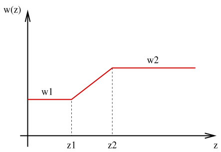
Figure 2: The four-parameter ansatz for $w(z)$ used in this analysis.

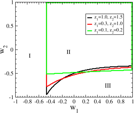
Figure 3: The fate of the universe as a function of $w_{1}$ and $w_{2}$ in our toy model. The results are fairly insensitive to $z_{1}$ and $z_{2}$, and are plotted for three pairs of these parameters. Region I: the universe is inflating now. Region II: the universe never inflated. Region III: the universe inflated, but then stopped inflating.

As Fig. 3 shows, there are three interesting regions of parameter space.

• Region I: Here $w_{1}<-1/(3\Omega_{X})$, and hence the universe is undergoing inflation today independent of the behavior of $w(z)$ at higher $z$.

• Region II: Here $w_{1}$ is too high for inflation to be occurring today, and $w_{2}$ is too high for inflation to have occurred in the past, cf. Eq. (5). Hence, our patch of the universe never underwent late-time inflation.

• Region III: Here $w_{1}$ is too large for inflation to be occurring now, but $w_{2}$ is negative enough that the universe recently inflated but then stopped inflating.

Note also the $z_{1}$ and $z_{2}$-dependent “dip” at $w_{1}$ just greater than $-0.48$. This feature can be explained simply. If $w_{1}=-0.45$, say, then dark energy becomes subdominant to dark matter with increasing redshift, and it takes a very negative $w_{2}$ (close to $-1$) to achieve inflation in the past. However, if $w_{1}$ is more positive, $+1.0$ say, dark energy is not as subdominant at higher $z$ (or perhaps is dominant), and it takes a less negative $w_{2}$ to achieve inflation in the past.

IV Observing the contraction of the MAS?

Let us begin by generalizing the condition of STV Starkman:1999pg for the observability of the turnaround point of the MAS. The redshift of the turnaround $z_{c}$ (where ‘c’ stands for ‘contraction’) is given by

$$Q(z_{c})=0,$$ (7)

where $Q(z)$ is given in Eq. (4) and $\rho_{X}(z)$ is given by Eq. (2). The condition for observing the turnaround point is given by

$$a_{c}\int_{\eta_{0}}^{\eta_{c}}d\eta=H^{-1}(\eta_{c})\ ,$$ (8)

which, when combined with Eq. (7) and for constant $w$, simplifies to

$$\int_{a_{c}}^{1}{dx\over\sqrt{x^{3}(x^{3w}-1-3w)}}={1\over\sqrt{-3w}}\ ,$$ (9)

where $a_{c}$ is the scale factor at turnaround (normalized to 1 today).

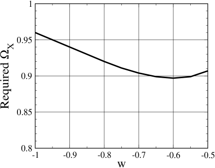
Figure 4: The required minimum value of $\Omega_{X}$ in order for us to be able to observe the turnaround point of the MAS today. Shown as a function of (constant) $w$.

We can now compute which models allow the turnaround to be observable (that is, $a_{c}<1$). Solving Eq. (9) numerically for $a_{c}$ and combining with Eq. (7), we find that, to a good approximation, the constraint from STV is roughly independent of w; see Fig. 4. Therefore, $\Omega_{X}\gtrsim 0.9-0.95$ would be necessary to directly observe the contraction of the MAS, with weak dependence of this value on $w$. Sadly, current data suggest that $\Omega_{X}\simeq 0.7$.

Figure 5: Spacetime diagram showing the MAS position ($r=H_{comov}^{-1}$) as a function of conformal time $\eta$. The universe undergoes inflation at $\eta>\eta_{c}$. On our present light-cone we observe supernovae (SNe) and the cosmic microwave background (CMB), while we presently can not observe the turnaround point of the MAS. The best we can do is observe points on our light cone that are causally connected with the turnaround point of the MAS. These points are denoted as $P_{v}$, where $v$ is the speed of signal at $P_{v}$ required for it in order to interact with the turnaround point. Three points are shown, for $v=-1$ (signal moving away from as at the speed of light), $v=0$ (signal at rest in comoving coordinates) and $0<v=v_{1}<1$.

Since the contraction of the MAS is currently unobservable, the best we can hope for is to observe points on our light cone that are causally connected with the turnaround point of the MAS. By making observations out to one of these points, call it $P$, we can verify (at least in principle) the continued presence of the dark-energy component (i.e., $\Omega_{X}(z)$ and $w(z)$). Having successfully done this, the only obstacle to concluding that the universe is inflating is that there could exist some physics, such as a domain wall separating our region of false vacuum from one of true vacuum, located at $P$ and which adds enough energy (with sufficiently positive pressure) at the turnaround point to spoil the contraction of the MAS, and hence inflation.

The redshift of these observable points $P$ can be computed for a given speed with which a signal located at that point (and observed by us) moves in order to reach the turnaround of the MAS some time later. In Fig. 5, these points are labeled as $P_{v}$, where $v$ is the speed of the signal in question ($v$ is in units of the speed of light $c$).

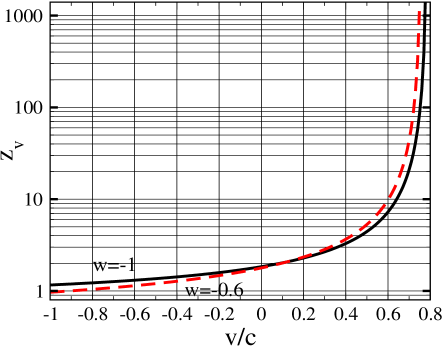
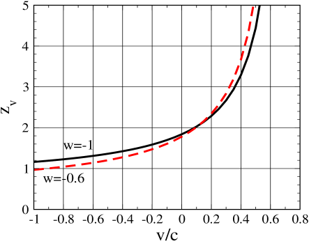
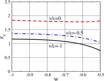
Figure 6: Top panel: $z_{v}$ computed as a function of $v$ for $w=-1$ and $w=-0.6$. Middle panel: Same as top panel, but now shown with low-$z_{v}$ region magnified. Bottom panel: $z_{v}$ computed as a function of $w$ for $v=0$, $-0.5$ and $-1$. All panels assume constant $w$.

From Fig. 5, the conformal distance and time at which we see these points is given by

$$r_{v} = {v(\eta_{0}-\eta_{c})-r_{c}\over v-1}$$ (10)

$$\eta_{v} = \eta_{0}-r_{v}\ ,$$ (11)

where $v$ is the velocity of the signal with respect to us, $r$ and $\eta$ are conformal distance and time respectively, and subscripts $0$ and $c$ denote today and at the contraction point of the MAS respectively. We have adopted the convention that $v=\pm 1$ denotes the signal moving directly toward (away) away from us (at the speed of light). Obviously, $r(v=1)=\infty$, since if $r(v=1)$ were finite, then the MAS would be on our light cone and we would be able to see it.

We solve Eqs. (10) and (11) numerically, and display the results in Fig. 6. The top and middle panels of Fig. 6 show the observable redshifts $z_{v}$ as a function of the speed of the signal $v$ for two different values of $w$. Note that $z_{v}$ increases rapidly as $v$ increases, going to infinity for $v\sim 0.8$, and is fairly insensitive to $w$. The bottom panel shows $z_{v}$ as a function of (constant) $w$ for three different values of $v$; for example, for $v=0$ and $-1<w<-0.5$, $z_{v}\approx 1.8$.

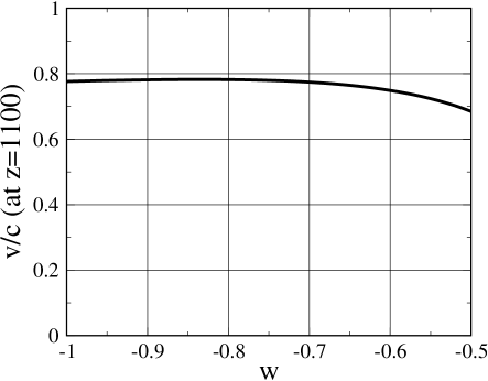
Figure 7: The requisite velocity of a signal located at the last scattering surface ($z\approx 1100$) in order for it to interact with the turnaround point of the MAS.

Now, when we look at the CMB sky, we observe photons that arrive from the last scattering surface (LSS). We compute the velocity with which a signal located at the LSS would have to propagate in order for the signal to interact with the turnaround point of the MAS, and hence affect the onset of inflation in our patch of the universe. We use Eqs. (10) and (11) to compute this velocity and its dependence on various cosmological parameters. Representative results are displayed in Fig. (7) in which we plot $v$ as a function of constant $w$, for fixed $\Omega_{X}=0.7$. Clearly, for any disturbance propagating at $v\gtrsim 0.8c$ it is impossible to rule out that this disturbance has prevented or ended a recent inflationary period.

V Conclusions

During the last few years there has been considerable excitement over a wide variety of data, most directly the observations of type Ia supernovae, strongly suggesting that on the scales that have been probed the rate of cosmic expansion is accelerating (or at least was at $z\simeq 0.5$). If correct, this implies that the energy density of the universe is (or was) dominated by dark energy – a component with negative pressure comparable to its energy density. The inferences that have been drawn – that the entire universe is currently in the throes of a new period of inflation of indefinite, and perhaps infinite, duration – rely on common but important simplifying assumptions: that the dark energy density is homogeneous out to at least the limit of the visible universe, and that the time evolution of the dark energy density, if any, is relatively slow, governed perhaps by the classical evolution of a scalar field in some smooth, flat, effective potential.

Unfortunately, as we have found, none of these inferences or assumptions are fully testable. The period of accelerated cosmic expansion has not lasted long enough for any observations, even in principle, to confirm that the local Hubble volume is vacuum-dominated and contained in the interior of an antitrapped surface – the condition that inflation is indeed taking place. Such observations, even assuming a homogeneous cosmological constant-dominated universe, will need to wait until the energy density of the cosmic vacuum has risen to about 95% of the critical energy density from its current 70%. If the assumption of spatial homogeneity is maintained, but the assumption of a static source of dark energy density is relaxed, then we find that inflation is underway in any epoch in which $w$, the effective equation of state of the dark energy over a Hubble volume, is sufficiently vacuum-like; $w<-1/(3\Omega_{x})$. Investigations of spatial inhomogeneities, particularly ones that could end any ongoing inflationary expansion, require observations of relatively small effects at relatively large distances. It is possible, in principle, to look out and tell whether a slow moving ($v\lesssim 0.8c$) disturbance will prevent our little corner of the universe from inflating. However, until $\Omega_{X}\simeq 0.95$, we cannot be completely confident that this inflation will ultimately begin and we can never tell how long it will last, since this depends on the future behavior of dark energy and its equation of state. The future of the universe remains uncertain.

- (1) A. G. Riess et al. [Supernova Search Team Collaboration], Astron. J. 116, 1009 (1998) [arXiv:astro-ph/9805201].
- (2) S. Perlmutter et al. [Supernova Cosmology Project Collaboration], Astrophys. J. 517, 565 (1999) [arXiv:astro-ph/9812133].
- (3) S. Perlmutter, M. S. Turner and M. J. White, Phys. Rev. Lett. 83, 670 (1999) [arXiv:astro-ph/9901052].
- (4) L. M. Wang, R. R. Caldwell, J. P. Ostriker and P. J. Steinhardt, Astrophys. J. 530, 17 (2000) [arXiv:astro-ph/9901388].
- (5) A. H. Guth, Phys. Rev. D 23, 347 (1981).
- (6) A. D. Linde, Phys. Lett. B 108, 389 (1982).
- (7) A. Albrecht and P. J. Steinhardt, Phys. Rev. Lett. 48, 1220 (1982).
- (8) J. Newman and M. Davis, Astrophys J. 534 , L11 (2000)
- (9) Z. Haiman, J. J. Mohr, and G. P. Holder, Astrophys. J. 553, 545 (2001)
- (10) D. Huterer, Phys. Rev. D., in press (astro-ph/0106399)
- (11) W. Hu, D. J. Eisenstein, M.Tegmark and M. White, Phys. Rev. D. 59, 023512 (1999)
- (12) G. Starkman, M. Trodden and T. Vachaspati, Phys. Rev. Lett. 83, 1510 (1999) [arXiv:astro-ph/9901405].
- (13) T. Vachaspati and M. Trodden, Phys. Rev. D 61, 023502 (2000) [arXiv:gr-qc/9811037].
- (14) P. P. Avelino, J. P. de Carvalho and C. J. Martins, Phys. Lett. B 501, 257 (2001) [arXiv:astro-ph/0002153].
- (15) E. H. Gudmundsson and G. Björnsson, arXiv:astro-ph/0105547.
- (16) B. Ratra and P. J. Peebles, Phys. Rev. D 37, 3406 (1988).
- (17) R. R. Caldwell, R. Dave and P. J. Steinhardt, Phys. Rev. Lett. 80, 1582 (1998) [arXiv:astro-ph/9708069].
- (18) C. Armendariz-Picon, V. Mukhanov and P. J. Steinhardt, Phys. Rev. Lett. 85, 4438 (2000) [arXiv:astro-ph/0004134].
- (19) C. Armendariz-Picon, V. Mukhanov and P. J. Steinhardt, Phys. Rev. D 63, 103510 (2001) [arXiv:astro-ph/0006373].
- (20) C. B. Netterfield et al. [Boomerang Collaboration], arXiv:astro-ph/0104460.
- (21) C. Pryke, N. W. Halverson, E. M. Leitch, J. Kovac, J. E. Carlstrom, W. L. Holzapfel and M. Dragovan, arXiv:astro-ph/0104490.
- (22) R. Stompor et al., Astrophys. J. 561, L7 (2001)
- (23) X. Wang, M. Tegmark and M. Zaldarriaga, astro-ph/0105091
- (24) M. S. Turner, Physica Scripta T85, 210 (2000)
- (25) P. G. Ferreira and M. Joyce, Phys. Rev. D 58, 023503 (1998)
- (26) D. Huterer and M. S. Turner, Phys. Rev. D 64, 123527 (2001)
- (27) J. Weller and A. Albrecht, astro-ph/0106079
- (28) J. Kujat, A. M. Lynn, R. J. Scherrer and D. H. Weinberg, Astrophys. J., in press (astro-ph/0112221)
- (29) R. Bean and A. Melchiorri, Phys. Rev. D., in press (astro-ph/0110472)