Heating of the intracluster medium by quasar outflows

Abstract

We study the possibility of quasar outflows in clusters and groups of galaxies heating the intracluster gas in order to explain the recent observation of excess entropy in this gas. We use the extended Press-Schechter formalism to estimate the number of quasars that become members of a group of cluster of a given mass and formation epoch. We also estimate the fraction of mechanical energy in the outflows that is imparted to the surrounding medium as a function of the density and temperature of this gas. We finally calculate the total amount of non-gravitational heating from such outflows as a function of the cluster potential and formation epoch. We show that outflows from broad absorption line (BAL) and radio loud quasars can provide the required amount of heating of the intracluster gas. We find that in this scenario most of the heating takes place at $z\sim 1\hbox{--}4$, and that this “preheating” epoch is at lower redshift for lower mass clusters.

1 Introduction

Clusters and groups of galaxies contain a large amount of hot gas, besides galaxies and the gravitationally dominant dark matter. This hot X-ray-emitting gas known as the intracluster medium (ICM) represents a part of the baryonic matter of the universe that is not associated with individual galaxies but remains trapped in the deeper gravitational potential of galaxy clusters. Hierarchical models of structure formation have been very successful in explaining many observed properties of galaxies and galaxy clusters. Nevertheless, some puzzling problems remain open and unexplained. Models of cluster formation in which the intergalactic gas simply falls into the dark matter dominated gravitational potential well (so-called infall models) fail to reproduce all the structural properties of the local cluster population (e.g., Evrard & Henry 1991; Navarro, Frenk & White 1995; Mohr & Evrard 1997; Bryan & Norman 1998). There is certainly some additional physics driving ICM evolution.

Recent X-ray observations have provided evidences for some non-gravitational heating of the diffuse, high density baryons in the potential wells of groups and clusters of galaxies, in addition to the heating during the gravitational collapse. One of the first evidences was in the shape of the $L_{x}-T$ relation, which is steeper than the self-similar behaviour $L_{x}\propto T^{2}$ predicted in the case of gravitational processes only. As early as the emergence of $ROSAT$ and $Einstein$ data, several authors proposed that the missing element is the existence of a “preheated high-entropy” intergalactic gas prior to a cluster’s collapse (David et al. 1991; Evrard & Henry 1991; Kaiser 1991; White 1991). Later, Ponman et al. (1999), and Lloyd-Davies et al. (2000) found direct evidence of an entropy excess with respect to the level expected from gravitational heating in the centre of groups. Ignoring the constant and logarithms, one can define the “entropy” as $S\equiv T/n^{2/3}$. The excess entropy, or equivalently, the excess specific energy, flattens the density profile decreasing the X-ray luminosity which is proportional to the square of the density. The effect is stronger in poorer clusters, where the excess energy associated with the excess entropy is comparable to the gravitational binding energy, while rich clusters, where gravity is dominant, are mostly unaffected. This produces a steepening of the $L_{x}-T$ relation.

The most popular scenario to successfully explain these thermal properties of the ICM has been the “preheating” scenario. For this scenario, the candidate processes which have been looked into are strong galactic winds driven by supernovae. However Valgeas & Silk (1999) showed that the energy provided by supernovae cannot raise the entropy of intergalactic medium (IGM) up to the level required by current observations. The observed amount of required energy injection depends on the epoch, and have been in the range of 0.4 - 3 KeV per gas particle (Navarro et al. 1995; Cavaliere et al. 1997; Balogh et al.1999; Wu et al. 2000; Lloyd-Davies et al. 2000, Borgani et al. 2001). For example, Wu et al. (2000) showed that galactic winds can impart only $\leq 0.1$ keV per particle. Moreover, Kravtsov & Yepes (2000) estimated the energy provided by supernovae from the observed metal abundance of ICM and found that the heating only by supernovae driven outflows requires unrealistically high efficiency. On the other hand, quasar outflows may be much more powerful and plausible candidates of the heating (Valageas & Silk 1999). In this paper, we focus on the role of quasar outflows in this regard.

The epoch of the energy input also remains uncertain. Lloyd-Davies et al. (2000) put an upper limit of $z_{max}\sim 7\hbox{--}10$ on the preheating epoch, from their estimate of excess entropy in groups. For AGNs, there have been no additional constraints like the metal abundance in the case of supernova heating (Kaiser & Alexander 1999). Recently, Yamada & Fujita (2001) have looked into the deformation of the cosmic microwave background (the Sunyaev-Zel’dovich effect) by hot electrons produced at the shocks produced by jets from AGNs. They showed that the observed excess entropy of ICM and $COBE/FIRAS$ upper limit for Compton $y$-parameter are compatible with each other only when the heating by jets occurred at relatively small redshift ($z\leq 3$). Thus they questioned the “preheating” scenario as their result suggests that the heating occurred simultaneously with or after cluster formation.

In this paper, we calculate the heat input from quasar outflows inside clusters. We calculate the mechanical work done by various kinds of quasar outflows and the excess energy imparted by them onto the intracluster medium via pdV work. For the statistics of quasars inside clusters, we use the extended Press-Schechter formalism. Finally we calculate the excess energy per particle and tally them with available observations.

In the next section, we discuss the abundance of quasars inside clusters of a given mass. We then discuss the evolution of quasar outflows and the mechanical work done by them in §3. We use these concepts to calculate the heating of the ICM in §4. We then discuss the implications of our results in §5. Throughout the paper we assume a flat universe with a cosmological constant, with $\Omega_{0}=0.35,\,\Omega_{\Lambda 0}=0.65,$ and $h=0.65$.

2 Quasars inside clusters

For a proper evaluation of the heat input from quasars inside clusters, one first needs to calculate their abundance and its dependence on the quasar mass, cluster mass, and the cluster formation redshift. Observationally, it is still difficult to obtain good statistics of quasars inside clusters. Estimation of the galaxy-QSO correlation function have shown that at low redshifts ($z\la 0.4$), quasars typically reside in small to moderate groups of galaxies and not in rich galaxies (e.g., Bahcall & Chokshi 1991; Fisher et al. 1996). It is still uncertain whether or not their optical or radio luminosities depend on their environments. Some studies (e.g., Ellingson, Yee & Green 1991) have shown that radio-loud quasars preferentially reside in richer clusters at higher redshift, although more recent studies (e.g., Wold et al. 2001) do not find any such correlation.

There has been, however, considerable work in relating the observed quasar luminosity function or the radio luminosity function (for radio-loud quasars) with the mass function of galaxies as prescribed by the Press-Schechter (PS) formalism (e.g., Haehnelt & Rees 1993; Haiman & Loeb 1998; Yamada, Sugiyama & Silk 1999).

At $z=0$, Yamada, Sugiyama & Silk found that one can reproduce the abundance of the radio sources powered by AGNs (i.e., leaving aside the radio sources powered by starbursts) by assuming that a fraction $f_{r}$ of the halos from PS formalism become radio-loud quasars, where, $f_{r}\sim 0.01$ for $M_{h}\ga 10^{12}$ M_⊙, and $f_{r}=0$ for $M<10^{12}$ M_⊙. They assume an upper limit on $M_{h}$ of $10^{14}$ M_⊙. Since it is known that radio loud quasars constitute a fraction $0.1$ of the quasar population (Stern et al. 2000), this means that a fraction $f_{q}=10f_{r}$ of the halos from PS formalism become quasars. In other words, $f_{q}\sim 0.1$ for $10^{12}\leq M_{h}\leq 10^{14}$ M_⊙, and $f_{q}=0$, otherwise. Yamada, Sugiyama & Silk (1999) assumed this fraction to be a constant for all redshifts. In this model, the rate of formation of quasars is given by the derivative of the PS mass function at the relevant mass scale.

This is similar to the model adopted by Haiman & Loeb (1998) and Furlanetto & Loeb (2001; FL01). FL01 showed that at high redshift ($z\ga 4$) the rate of formation of quasars is a fraction $f_{q}\sim 0.1$ of the rate of formation of halos from PS formalism, if a life time of order $10^{7}$ yr is assumed for the quasar. There is, however, a difference, in that they had only a lower limit to $M_{h}$ and no upper limits (see eqns (2) & (3) of Haiman & Loeb 1998). They mention that at low redshifts their formalism does not predict any decline as observed in reality, and for which they consider their model only at high redshift. It is possible that this mismatch is due to the lack of upper limits, since the the differentiation of PS mass function for objects with an upper limit in mass decreases at low redshift, (Haiman, Z. 2001, private communications). In any case, Haiman & Loeb (1998) found that this prescription yields a matching quasar luminosity function that is observed, at redshift $z\geq 2.5$. We find later that most of the heating of the ICM gas (even for our least massive cluster) occurs at $z\geq 2$ (Figure 7). We will therefore assume for simplicity that this fraction $f_{q}\sim 0.1$ at all redshifts (as in Yamada et al. 1999).

In this paper, we would like to have a conservative estimate of the quasar abundance. Also, we would like to calculate the abundance of quasars in clusters including low mass groups of galaxies. For this reason, we assume the value of $f_{q}$ as above, but use an upper limit of $10^{13}$ M_⊙. Since the mass function decreases steeply at the higher mass end, this should not change the value of $f_{q}$ substantially. In brief, we assume that,

$$f_{q}\sim\left\{\begin{array}[]{ll}0.1&\mbox{if $10^{13}\ga M_{h}\ga 10^{12}\,M_{\odot}$}\\ 0&\mbox{if $M_{h}>10^{13}\,M_{\odot}\,,M_{h}<10^{12}\,M_{\odot}\>,$}\end{array}\right.$$ (1)

motivated by the model of Yamada, Sugiyama & Silk (1999), and by the fact that a similar prescription by Haiman & Loeb (1998) recovers the quasar population at high redshift, and relate the rate of formation of quasars with that of halos in the PS formalism.

We are, however, concerned with the statistics of quasars inside clusters. For this one needs to have an extension of the PS mass function which can predict the probability of a given halo becoming a part of bigger object later, or the probability of an object having had a progenitor of a given mass at an earlier epoch. Such extensions of the PS theory have been studied in detail by Bower (1991) and Lacey & Cole (1993), for example.

In the standard PS theory, the mass function, i.e., the fraction of regions with mass in the range $M,M+dM$ which have overdensity $\delta$ in excess of $\delta_{c}$ (which is the threshold for perturbations becoming non-linear), is given by,

$$f_{PS}=f(M,\delta_{c})dM={-1\over\sqrt{2\pi}}{\delta_{c}\over(\sigma_{M}^{2})^{3/2}}\exp\Bigl{[}-{\delta_{c}^{2}\over 2\sigma_{M}^{2}}\Bigr{]}{d\sigma_{M}^{2}\over dM}dM\,.$$ (2)

Here, $\sigma_{M}$ is the mass variance of the perturbation at the mass scale $M$. The relation between the number density of objects in the mass range $M,M+dM$ with $f(M)dM$ is,

$$n(M)dM={\rho_{o}\over M}f(M)dM\,,$$ (3)

where $\rho_{o}$ denotes the background mass density.

In the extended PS theory, the fraction of regions of mass $M$, contained within a larger scale region of mass $M^{\prime}$ and overdensity $\delta^{\prime}$, which are more overdense than $\delta_{c}$, is given by,

$$f(M,\delta_{c}|M^{\prime},\delta^{\prime})dM ={-1\over\sqrt{2\pi}}{(\delta_{c}-\delta^{\prime})\over(\sigma_{M}^{2}-\sigma_{M^{\prime}}^{2})^{3/2}}$$ (4)

$$\times\exp\Bigl{[}-{(\delta_{c}-\delta^{\prime})^{2}\over 2(\sigma_{M}^{2}-\sigma_{M^{\prime}}^{2})}\Bigr{]}{d\sigma_{M}^{2}\over dM}dM\,.$$

This expression recovers the simple PS mass function in the limit $M^{\prime}\rightarrow\infty$ and $\delta^{\prime}\rightarrow 0$, relevant for the whole universe.

If we then identify $M^{\prime}$ with $M_{cl}$, the mass of a cluster, and $\delta^{\prime}=\delta_{c}(z_{f})$, the threshold overdensity of the cluster at its formation epoch $z_{f}$, we can then obtain the mass fraction of $M_{cl}$ which have been parts of progenitors of a given mass range ($M$ to $M+dM$) at a given (earlier) redshift. If we also identify this mass range with that of the quasars as in the standard PS theory ($10^{12}\hbox{--}10^{13}$ M_⊙), and use the fraction of these halos that become quasars ($f_{q}$; eqn 1), we will obtain the mass fraction of the final cluster which have been quasars at some given earlier epoch.

To obtain the rate of formation of these quasars (inside a future cluster of mass $M_{cl}$), we should differentiate the above expression. A simple differentiation will, however, not give the correct result, since there will be a negative contribution from the merging of halos out of this mass range. One would get a negative rate of formation of such quasars at some point if the rate at which they disappear beyond this mass limit is not taken into account in a proper manner. This

Consider the abundance of objects in a given mass range $M,M+dM$ at two successive epochs $z_{1}$ and $z_{2}$ ($z_{2}<z_{1}$). The abundance $f(M)dM$ at $z_{2}$ will be given by $f_{2}=f_{1}+F-D$, where $f_{2}$ and $f_{1}$ are the abundances at epochs $z_{2}$ and $z_{1}$, the term $F$ denotes the abundance of newly formed objects in this mass range during the epoch $z_{1}$ and $z_{2}$ (from merger of smaller objects), and $D$ signifies the abundance of objects that moved out of this mass range as a result of merger (into bigger objects). A simple differentiation of the PS function, involving the difference $(f_{2}-f_{1})$ will therefore depend on both $F$ and $D$. For a given range of mass, $D$ is very small at a very early epoch, but it increases with time (see, e.g., Fig. 5 of Haiman & Menou 2000), and at a later epoch can become larger than $F$. Therefore, at lower redshifts, a simple differentiation can imply a negative rate of change of abundance. If the contribution of $D$ is neglected, one would then incorrectly get a negative value of $F$.

This problem has been encountered in the case of ordinary PS function by many authors. While studying the rate of mergers in the context of background radiation from starbursts and AGNs, Blain & Longair (1993) noted that a simple differentiation of the PS function leads to a negative rate of formation of objects in a given mass range. In other words, the actual rate of formation of objects is given by,

$$\dot{f}_{form}=\dot{f}_{PS}+\dot{f}_{merger}\,.$$ (5)

They performed a simulation assuming a simple power spectrum and obtained a fit for the rate of these objects merging to form bigger objects. They found that $\dot{f}_{merger}$ can be approximated well (in the Einstein de-Sitter universe) by,

$$\dot{f}_{merger}=\phi{f_{PS}\over t}\exp\Bigl{[}(1-\alpha){\delta_{c}^{2}\over 2\sigma^{2}}\Bigr{]}\,$$ (6)

where the value of $\alpha\sim 1.35$ and $\phi\sim 1.3\hbox{--}1.7$. This problem has also been investigated by Sasaki (1994) and Percival & Miller (1999). With the extension of the PS formalism, one can now calculate this merging rate (see also, Chiu & Ostriker 2000).

We note here that in the case of the merger of a lower mass quasar into a more massive quasar, our implicit assumption is that the central black holes also merge and form a bigger black hole appropriate for the bigger quasar (see below; eqn 13). In other words, we assume that the central black hole mass always traces the halo mass.

The rate at which an object of mass $M$ at epoch $z$ merges to form a bigger object of mass $M^{\prime}$ is given by (Bower 1991; Lacey & Cole 1993),

$${d^{2}p\over dM^{\prime}dz}(M\rightarrow M^{\prime}|z)dM^{\prime} = {1\over\sqrt{2\pi}}{\sigma_{M}^{2}\over\sigma_{M^{\prime}}^{2}(\sigma_{M}^{2}-\sigma_{M^{\prime}}^{2})^{3/2}}$$ (7)

$$\times\exp\Bigl{[}-{\delta_{c}(z)^{2}(\sigma_{M}^{2}-\sigma_{M^{\prime}}^{2})\over 2\sigma_{M}^{2}\sigma_{M^{\prime}}^{2})}\Bigr{]}$$

$$\times|{d\sigma_{M}^{2}\over dM}||{d\delta_{c}(z)\over dz}|dM\,.$$

Here, $p(M\rightarrow M^{\prime}|z)dM^{\prime}$ is the probability of an object of mass $M$ merging to become an object of mass within the range $M^{\prime},M^{\prime}+dM^{\prime}$ at redshift $z$. The rate of disappearance of objects of a given mass, $\dot{n}_{merger}$, should be essentially,

$${df_{merger}\over dz}(M,z)=f_{PS}(M,z)\int_{2M}^{\infty}{d^{2}p\over dM^{\prime}dz}(M\rightarrow M^{\prime}|z)dM^{\prime}\,,$$ (8)

where the lower limit of the integration is chosen to be such that the merged object is at least twice as massive as the merging object. We show the result of this integration for a sCDM universe (with a COBE normalized power spectrum) in Figure 1, and show the fit of Blain & Longair with $\phi=0.9$ and $\alpha=1.35$. We find that the merging rate is fit by a lower value of $\phi$ than they assumed, although the difference is a factor of order unity. It is possible that this difference is due to the specific assumption in the simulation done by Blain & Longair (1993), e.g., in the power spectrum being a simple power law (Blain, A. 2001, private communication), or it can be a result of the lower limit ($2M$) chosen by us. At any rate, if we chose the above integral to represent the merger rate then it would be a conservative estimate, since decreasing the lower limit would simple increase the value of the merger rate, and in turn, the formation rate of objects.

Figure 1: The rate of disappearance of objects is compared in different cosmologies. The thin solid line shows the result of integration in eqn (8) for a SCDM universe for $M=10^{14}\,M_{\odot}$ and the dotted line shows the Blain & Longair (1993) fit with $\phi=0.9$ and $\alpha=1.35$. The thick solid line shows the result of the integration in the $\Lambda$CDM universe and the dashed line refers to a fit described in the text. Both curves use 4-year COBE normalized spectra.

We have found that the result in the case of the $\Lambda$CDM universe can be fit by a similar function, with $\phi$ being replaced by $0.9\,{d\delta_{c}(z)\over dz}$, for $\alpha=1.35$ with an accuracy of order $\la 5\%$. We, however, do not use these fits in our calculation, and evaluate the integral numerically for our purpose.

To be precise, this rate of disappearance is valid for the objects following the PS mass function, i.e., for objects which are not already parts of bigger objects. Motivated by the extension of the PS formalism, we here posit that the rate of disappearance of objects inside a bigger object also has the same form, with $f_{PS}(M,\delta_{c})$ in eqn (8) being replaced by $f(M,\delta_{c}|M^{\prime},\delta^{\prime})$. There is admittedly no way of verifying the truth of this ansatz at present, since this would involve more extensions of the PS theory than that is available now. It will also involve comparing the merger rates inside and outside of clusters. It, however, leads to a conservative estimate for the formation rate of quasar in a cluster. As the work of Bower (1991) has shown, growth of perturbations inside a cluster is enhanced compared to in the field. This means that the merging rate of objects of a given mass inside a cluster should be larger than that in the field. Here, by assuming a comparable merging probability (the factor that multiplies the abundance of objects, given by $f_{PS}$), we are in a way underestimating the rate of disappearance ($\dot{f}_{merger}$), and in turn, the rate of formation ($\dot{f}_{form}$) of quasars in a cluster. The final result of total heat input from our formalism should, therefore, be a conservative estimate.

Figure 2: The net formation rate of objects (${df_{form}\over dz}$) is plotted for objects of mass $10^{13}$ M_⊙ (for $dM=M$), in clusters (bottom panels, with $M_{cl}=10^{15}$ M_⊙) and in general (top panels), for sCDM (left panels) and $\Lambda$CDM (right panels) models. Dashed lines show the term ${df_{PS}\over dz}$, dotted lines show ${df_{form}\over dz}$ using the Blain & Longair fit (with $\phi=1.0$), and solid lines show ${df_{form}\over dz}$ using the integral in equation 8. The long-dashed line in lower right panel shows the case for $M_{cl}=10^{14}$ M_⊙.

We show the results of adding the rate of disappearance in Figure 2. The dashed lines, which show the term $-(df_{PS}/dz)$ (or equivalenlty, ${df_{PS}\over dt}$), become negative at lower redshift, suggesting the need for the addition of the rate of disappearance of objects. The dotted lines show the result of adding this rate, using the Blain & Longair (1993) fit (with $\phi=0.9$), and the solid lines show the result using the integral in equation 8. The upper panels of the figure show the case of objects (of mass $10^{13}$ M_⊙) in the field, and the bottom panels show the case for these objects inside a cluster of $M_{cl}=10^{15}$ M_⊙ ($z_{f}=0$). For these curves, we have used the integration in equation 8, and the extension of the PS mass function for the abundance of objects inside the cluster, as explained above. The left and right panels show the cases for sCDM and $\Lambda$-CDM universe. As the bottom panels show, the addition of the disappearance rate does not suffice to make $[-(df_{PS}/dz)]$ (inside clusters) positive at low redshift. This is suggestive of the enhanced growth of perturbation, and the need for a larger rate of merger inside clusters, as previous authors have noted.

We also show the case for $M_{cl}=10^{14}$ M_⊙ by the long dashed line in the lower right panel of Figure 2. Comparison with the solid line (for $M_{cl}=10^{15}$ M_⊙) shows that the formation rate of these galaxies inside a lower massive cluster is larger. This follows simply from the extension of the PS formalism (from the dependence on the term $(\sigma_{M}^{2}-\sigma_{M^{\prime}}^{2})$). It is interesting to note that this is consistent with the suggestion from observation that quasars are preferentially located in groups of galaxies instead of rich clusters (e.g., Bahcall & Chokshi 1991; Fisher et al. 1996).

If our formalism is used without any correction, this will lead to subtraction of energy input in the final result. We circumvent this problem by putting $[-(df_{PS}/dz)]=0$ when this term turns negative. This will, therefore, provide a lower limit to the total energy input from quasar outflows in a cluster.

We can finally write down the rate of formation of quasars in a given mass range $M,M+dM$ inside a cluster of a given mass, $M_{cl}$, in the form of the rate of increase of the fraction of mass of $M_{cl}$ which is in quasars at an epoch $z$, as (remembering the equation 3),

$${df_{q,cl}(M,z|M_{cl},z_{f})\over dz} dM=f_{q}\,{df(M,\delta_{c}(z)|M_{cl},\delta_{c}(zf))\over dz}dM$$ (9)

$$+f_{q}f(M,\delta_{c}(z)|M_{cl},\delta_{c}(zf))dM$$

$$\times\int_{2M}^{M_{cl}}{d^{2}p\over dM^{\prime}dz}(M\rightarrow M^{\prime}|z)dM^{\prime}\,,$$

with the condition that ${dn_{q}\over dz}=0$, for $z<z_{n}$, where ${dn_{q}\over dz}|_{z<z_{n}}>0$. The integral on the right hand side is evaluated using eqn(7). Here we have also changed the upper limit of the integration to $M_{cl}$. The integrand is a rapidly decreasing function of $M^{\prime}$ and the value of the integral depends mostly on the lower limit.

Here, the threshold density contrast in a cosmological constant dominated universe is given by a fit given by Kitayama & Suto (1996),

$$\delta_{c}(z)=1.68[g(z=0)/g(z)][1+0.0123\log\Omega_{m}(z)]\,.$$ (10)

In our calculations, we have used a fit for $g(z)$ from Carroll, Press & Turner (1992),

$$g(\Omega_{m}(z),\Omega_{\Lambda}(z))$$

$$\sim{5\Omega_{m}(z)\over 2[\Omega_{m}(z)^{4/7}-\Omega_{\Lambda}(z)+(1+{\Omega_{m}(z)\over 2})(1+{\Omega_{\Lambda}(z)\over 70})]}\,,$$ (11)

where (Lahav et al. 1991),

$$\Omega_{m}(z) = \Omega_{m0}(1+z)^{3}/[\Omega_{m0}(1+z)^{3}+\Omega_{\Lambda 0}]\,,$$

$$\Omega_{\Lambda}(z) = \Omega_{\Lambda 0}/[\Omega_{m0}(1+z)^{3}+\Omega_{\Lambda 0}]\,.$$ (12)

We emphasize here that the above formalism leads to a conservative estimate of abundance of quasars in a cluster (and, therefore, the final heat input), because (a) we ignore the increased pace of growth of perturbation and the merging rate inside a cluster, and (b) the lower limit of the integration could in reality be smaller than $2M$, which is probably the reason the rate of formation still turns negative at low redshifts even after the addition of merger term.

To summarise the work in this section, we have used the existing ideas for relating the quasar formation rate to the Press-Schechter mass function, to estimate the rate of formation of quasars inside clusters (as a function of cluster mass and formation redshift), utilizing the extensions of PS formalism. First, we use eqn (1) to relate the PS mass function to quasar abundance. The standard PS mass function (eqn 2) is then replaced by its extension (eqn 4). Furthermore, we add the contribution due to merger (into larger objects) (eqns 5 & 8), again using the extensions of PS mass function. We finally have the rate of formation of quasars inside clusters as given by eqn (9).

We use this formalism to calculate the total energy input from outflows from quasars in a cluster, or, a lower limit to it. We next discuss the energy input from individual outflows, which we will combine with our calculation of formation rate of quasars for the final result.

3 Work done by quasar outflows

In this section we calculate the energy input from quasar outflows into the ambient medium. We model the outflows as they evolve in the ambient medium and calculate the pdV work done by the outflows. To begin with, we discuss different kinds of outflows that we consider and the characteristics of the hosts of quasars.

3.1 Quasar outflows

We consider two major types of quasar outflows. For radio-loud quasars (RLQ), the outflow is in the form of a tightly collimated jet, which deposits energetic particles into a cocoon which expands against the surrounding medium. These outflows are characterised by the kinetic luminosity of the jet, $L_{k}$. According to Willot et al. (1999), this is correlated with the bolometric luminosity $L_{bol}$ of the quasar, and that $0.05\la L_{k}/L_{bol}\la 1.0$. We follow FL01 in arguing that since $L_{bol}\sim 10L_{B}$ (Elvis et al. (1994)), the rest-frame B-band luminosity, $L_{k}\sim L_{B}$.

Radio-loud quasars, however, constitute only about $10\%$ of the total population of quasars (Stern et al. 2000). We therefore define a factor $f_{o}$ for the fraction of quasars with outflows, and define $f_{o}\sim 0.1$ for our RLQ model. The fraction $f_{o}$ here denotes the number of radio relics/lobes per halo, since a radio loud quasar may have several outbursts of radio activity. This fraction is therefore a very conservative estimate since it is obtained from observed radio luminosity function and does not take into account the existence of radio relics in clusters.

Another important kind of outflows are encountered in broad absorption line (BAL) quasars. The absorption troughs are thought to be due to absorbing clouds flowing out of the quasars with velocities up to $0.1c$. Although they are encountered in about $10\%$ of the quasars, it is believed that all quasars have such outflows (all the time) and the covering fraction of the BAL outflows is about $10\%$ (Weymann et al. 1991; Weymann 1997). Some authors also believe that BAL outflows have a limited lifetime (especially the low ionization BALs) and that they have a large covering fraction in the early phase of a quasar (Voit et al. 1993). For our calculation, we use a fraction $f_{o}\sim 1$ for the BAL outflows. We discuss the effect of the uncertainty in these factors on the final result in §5.

We model the BAL outflows as having a kinetic luminosity $L_{k}$. Following FL01, if $N_{H}$ is the column density of the absorbing gas, $f_{c}$ the covering fraction, and $R_{BAL}$ is the size of the absorption system, then $L_{k}$ is related to the outflow velocity $v_{BAL}$ as $L_{k}\sim 2\pi f_{c}N_{H}m_{p}R_{BAL}v_{BAL}^{3}$. The observed range of these parameters are as follows: $v_{BAL}\la 0.1c$, $f_{c}\sim 0.1$ (Weymann 1997; but see above), $R_{BAL}\sim 1\hbox{--}500$pc and $N_{H}\sim 10^{22}\hbox{--}10^{23}$ cm^-2 (Krolik 1999; Gallagher et al. 1999). For these values, the magnitude of $L_{k}$ is close to that of $L_{B}$. FL01 also argued that for BAL winds $L_{k}\sim 0.1\hbox{--}100L_{B}$, and finally assumed $L_{k}\sim L_{B}$. Since this estimate depends crucially on a number of uncertain parameters (for example, the fact that the absorption column density in optical measurement is much smaller than the above mentioned X-ray column density), it may not really be a conservative estimate, but it does provide a simple scaling which we hope is not too unreasonable. The estimate $L_{K}\sim L_{B}\sim 0.1L_{Edd}$ is probably not a conservative estimate, but an upper limit, in that for a covering fraction of $10\%$, the mechanical luminosity of the wind could not be larger than $0.1$ of the Eddington rate. Keeping all these uncertainties in mind, we assume that $L_{k}\sim L_{B}$ for BAL outflows.

We then need to connect $L_{B}$ of a given quasar with the properties of its halo. Firstly, as Haiman & Loeb (1998) have shown, the mass of the black hole at the centre is related to $L_{B}$, as,

$$M_{BH}={1\over 0.093}\Bigl{(}{L_{B}\over 1.4\times 10^{38}\,{\rm erg}\,{\rm s}^{-1}}\Bigr{)}\,M_{\odot}\,$$ (13)

assuming that the quasar radiates at the Eddington luminosity. The factor of $0.093$ reflects the fraction of the Eddington luminosity radiated in the B-band, taken from the median quasar spectrum of Elvis et al. (1993). Statistically speaking, we therefore assume that a fraction $f_{q}$ (eqn(1)of all black holes radiate at the Eddington rate for a life time of $\sim 10^{7}$ yr, while the rest does not radiate at all.

Secondly, the correlation between the central black hole mass and the total baryonic mass of the galaxy (Magorrian et al. 1998; Gebhardt et al. 2000) gives $M_{BH}\sim 4\times 10^{-4}M_{h}$, where $M_{h}$ is the total mass of the galaxy, using a value of $M_{BH}/M_{baryonic}\sim 2\hbox{--}3\times 10^{-3}$, and $M_{baryonic}/M_{h}\sim\Omega_{b}/\Omega_{0}\sim 0.2$.

As far as the collimation is concerned, the geometry of BAL outflows is still uncertain, whereas the radio jets are well collimated. Since some models do suggest a modest collimation even in BAL outflows, with a covering fraction of $f_{c}\sim 0.1$ (Weymann 1997), we use the idea of collimated outflows for outflows from both radio-loud and BAL quasars.

We next discuss the evolution of the outflows from radio-loud quasars and calculate the fraction of its total kinetic luminosity that it deposits into the surrounding medium in the form of pdV work. For concreteness, we will assume that the corresponding fraction for BAL outflows has similar values, and keep in mind the uncertainty in the geometry and energetics of BAL outflows.

3.2 Evolution of outflows

The standard scenario for outflows from radio loud quasars involves a ‘cocoon’ surrounding the core and the jet, and consisting of a shocked ambient medium and shocked jet material (Scheuer 1974; Blandford and Rees 1974). Begelman & Cioffi (1989) constructed a simple model of the evolution of a cocoon in which the cocoon is overpressured against the ICM. In their model, the expansion along the jet axis is determined by the balance of the thrust of the jet and the ram pressure, whereas the thermal pressure of the cocoon drives along the direction perpendicular to the jet axis. Results of numerical simulations agree with this scenario (Loken et al. 1992; Cioffi & Blondin 1992).

Here we adopt the model of the evolution of cocoons following the approach of Bicknell et al. (1997), which is based on the Begalman & Cioffi (1989) model but includes the pdV work done by the cocoon, in order to find the fraction of total energy lost by the quasar to the ICM through mechanical work (pdV work). Bicknell et al. (1997) derived this fraction ($f_{pdV}$) to be $f_{pdV}=3/8$, for a homogeneous ambient medium (their equation (2.13)).

We will, however, calculate this fraction from numerical solution of the equations governing the evolution of the cocoon, for the following reasons. Firstly, the derivation mentioned above implicitly assumes that the mean pressure averaged over the hotspot region is equal to the mean lobe pressure (in the language of Bicknell et al. (1997), this means $\zeta\sim 1$). In fact, their equation (2.13) shows that for constant $\zeta$, one has in general, $P_{c}{dV_{c}\over dt}=(1+2\zeta)L_{j}/8\zeta$, which recovers the fraction $3/8$ for $\zeta=1$. In reality, however, this ratio does not remain a constant in time. Secondly, this derivation is valid only during the period when the jet is active. Even after the jet switches off, the cocoon, however, continues to evolve as a result of its overpressure until it reaches an equilibrium pressure with the ambient medium (see also Nath 1995). The cocoon, therefore, continues to do pdV work even after the jet switches off, and the inclusion of this process will lead to an upward revision of the fraction of total energy that is lost in pdV work. Besides, there seems to be some confusion in the literature regarding the fraction. For example, Inoue & Sasaki (2001) have recently adopted a fraction $f_{pdV}=1/4$ in their calculation of energy input into the surrounding gas.

We therefore calculate this fraction by numerically solving the equations of cocoon evolution.

We consider two collimated steady jets advancing into the ambient ICM. The thermalized jet matter and the shock-compressed ICM matter form a cocoon around the jets and the cocoon expands with shocks advancing in directions both parallel and perpendicular to the jet axis. After this stage of evolution, when the jet turns off after a lifetime of $t_{life}\sim 3\times 10^{7}$ years (Kaiser 2000), cocoons still retain high pressure. They cool radiatively and expand due to its overpressure till it reaches a pressure equilibrium with the ambient medium. Thus the relevant equations are:

$${dr_{h}\over dt} = \Bigl{(}{L_{j}\over A_{h}\rho_{a}\beta c}\Bigr{)}^{1/2},\qquad t<t_{life}$$ (14)

$$= \Bigl{(}{P_{c}\over\rho_{a}}\Bigr{)}^{1/2},\qquad t>t_{life}$$

$${dr_{c}\over dt} = \Bigl{(}{P_{c}\over\rho_{a}}\Bigr{)}^{1/2},$$ (15)

$${dE_{c}\over dt} = L_{j}-P_{c}{dV_{c}\over dt}$$ (16)

where $L_{j}$ is the jet luminosity, $\rho_{a}$ is the density of the ambient medium and $\beta c$ is the velocity of the jet material. As the jet is highly relativistic, $\beta\sim 1$. The averaged hotspot area $A_{h}\sim 30$ kpc² (Bicknell et al. 1997) is assumed to be larger than the radius of the jet, according to the ‘dentist’s drill’ model of the jet (Scheuer 1982). Here $r_{h}$ is the length of the jet or the distance of the hotspot from the centre of the galaxy, $r_{c}$ is the half-width of the cocoon at the centre and $V_{c}$ is the volume of the cocoon given by $V_{c}=\epsilon_{v}(2\pi r_{c}^{2})r_{h}$ where $\epsilon_{v}$ is the geometrical factor depending on the shape of the cocoon. For our calculations we have taken the shape of the cocoon as biconical and so $\epsilon_{v}\sim 1/3$. Finally $P_{c}$ is the pressure inside the cocoon given by $P_{c}=(E_{c}/V_{c})(\gamma-1)$ where $\gamma=4/3$ and $E_{c}$ is the total energy inside the cocoon given by $E_{c}=L_{j}t$ till $t<t_{life}$ and $E_{c}=L_{j}t_{life}$ afterwards, where $t_{life}$ is the lifetime of the jet.

This is admittedly a simplified model of the evolution of the cocoon. In reality, after the jet switches off, one expects Rayleigh-Taylor and Kelvin-Helmholtz instabilities to distort the cocoon, giving rise to ‘buoyant’ plumes. This phase of the evolution of the cocoon, and its effect on the ambient medium, has been recently addressed by various authors (Gull & Northover 1973; Churazov et al. 2000; Brüggen & Kaiser 2000), mainly with the help of numerical simulations. It is possible that this phase adds substantial heating to the intracluster medium, but short of doing a numerical simulation it is difficult to assess its importance. We have also neglected the loss of energy through radiation, as modeling such losses would involve detail knowledge of various parameters (e.g., electron energy spectrum and the possibilities of re-acceleration of electrons). With the uncertainties involved in modeling these process, it seems reasonable to adopt the above simplified picture as a pointer and keep the uncertainties in mind while discussing the final result. In light of this discussion, we will also calculate the final result with a value of $f_{pdV}=3/8$ as in Bicknell et al. (1997), which we will adopt as a conservative lower limit.

Figure 3: The dependence of $f_{pdV}$ with the ambient density $n$ is shown for various ambient temperatures $T$ for various $L_{k}$ (erg/s) with and without radiation loss. Solid and dashed lines are for $L_{k}=10^{46}$ erg/s and $10^{47}$ erg/s respectively without radiation loss. Dotted lines are for $L_{k}=10^{46}$ with radiation loss.

We numerically calculate the volume of the cocoon as it grows into the ICM and the pressure inside the cocoon at each step, and add up the pdV work to get the final amount of energy lost in this mode. The evolution of the cocoon is continued until the pressure inside the cocoon becomes equal to the ambient pressure, $n_{a}k_{B}T_{a}$ ($n_{a}=\rho_{a}/\mu m_{p}$), where $T_{a}$ is the temperature of the ICM. The fraction $f_{pdV}$ is calculated by taking the ratio of the total energy lost through mechanical work to the total energy (that is $L_{j}t_{life}$). (We found that for the relevant values of the ambient medium parameters, the time scale to reach pressure equilibrium is always larger than $t_{life}$.) The dependence of $f_{pdV}$ on the ambient density, is shown in Figure 2 for $T_{a}=10^{6},10^{7}$ and $10^{8}$ K, and for $L_{k}=10^{46}$ (solid lines) and $10^{47}$ erg/s (dashed lines).

The plot shows that the fraction $f_{pdV}$ is a function of temperature of the cluster and also the density of the ambient medium. The general trend is that the fraction reduces at higher temperatures and higher densities. This is because of the fact that the cocoon reaches pressure equilibrium with the ambient medium sooner for a higher pressure environment (higher $T_{a}$ and $n_{a}$), and the total pdV work ends up being smaller. The plot also shows that the fraction $f_{pdV}$ depends weakly on the jet luminosity for lower temperatures ($T_{a}\leq 10^{7}$ K), whereas there is a bit of a difference for $T_{a}\sim 10^{8}$ K.

The fraction $f_{pdV}$ calculated above is somewhat larger than that has been used in the literature, for ambient medium with low pressure. The difference is mainly the result of our inclusion of cocoon evolution even after the jet has switched off. Incidentally, Inoue & Sasaki (2001), while using a value of $f_{pdV}=1/4$, discussed the possibility that this fraction could be larger in reality, because of its continued evolution after the switching off of the jet (their §3.2).

In our calculation for the total pdV work done by BAL and RLQ outflows, we will use the values of $f_{pdV}$ obtained above. As mentioned earlier, the energetics and geometry of BAL outflows are not clear at present. For concreteness, we have worked out the case of RLQ outflows in detail, and we will use the same values of $f_{pdV}$ for BAL outflows as well.

4 Heating of the ICM

Equipped with the knowledge of the rate of formation of quasars in clusters (equation 9) and the fraction of total energy which is deposited as pdV work by the outflows from them (§3.2), we are now in a position to calculate the total amount of non-gravitational energy provided by quasar outflows in a cluster. If we denote the gas fraction of the total cluster mass by $f_{gas}$, then the total number of gas particles is $\sim M_{cl}f_{gas}/m_{p}$, where $m_{p}$ is the proton mass. It is not yet clear if the gas fraction has a universal value for clusters of all masses and at all redshifts. A few authors (see, e.g., Schindler (1999)) have found no correlation of the gas fraction with the cluster mass, whereas others (e.g., Ettori & Fabian (1999)) find some correlation (with low mass clusters possessing lower gas fraction). This correlation has been attributed to the excess energy deposition (since low mass clusters are more liable to lose gas from heating than massive clusters) (see, e.g., Bialek et al. (2000)). Here, we are, however, trying to calculate the magnitude of this very excess energy. It would not be appropriate to include this correlation it a priori in our calculation. (We show later that including these correlations only increases our estimate of excess energy input.) We have, therefore, used a value of $f_{gas}=0.1$ for our calculation. The total energy per (gas) particle deposited into the ICM of a cluster of mass $M_{cl}$ is then given by,

$$\epsilon_{pdV}= {m_{p}\over M_{cl}f_{gas}}\int_{z_{m}}^{0}\int_{M_{l}}^{M_{u}}{df_{q,cl}(M,z|M_{cl},z_{f})\over dMdz}$$ (17)

$${M_{cl}\over M}dM\,dz\,f_{o}\,[L_{k}t_{life}f_{pdV}(n_{a},T_{a})]\,,$$

where $\Bigl{[}{d^{2}n_{q}(M,z|M_{cl},z_{f})\over dMdz}dMdz\Bigr{]}$ is calculated using equation 9. The factor $f_{o}\sim 1$ for the BAL outflows, and $f_{o}\sim 0.1$ for outflows from RLQs (§3). The redshift $z_{m}$ is the maximum redshift of heat input. We later show (Figure 7) that the heat input is negligible for $z\geq 5$. The density and temperature of the ICM of a cluster of a given mass ($M_{cl}$) and formation redshift ($z_{f}$) is calculated using (Eke et al. 1998),

$$T_{a}=1.65\times 10^{7}(1+z)\Bigl{[}{M_{cl}\over 10^{15}h^{-1}\,M_{\odot}}\Bigr{]}^{2/3}\Bigl{[}{\Omega_{0}\Delta(\Omega_{0},z)\over\Omega(z)}\Bigr{]}^{1/3}\,,$$ (18)

and,

$$n_{a}={M_{cl}f_{gas}\over m_{p}(4/3)\pi r_{vir}^{3}}\,,$$ (19)

where

$$\Delta(z)=18\pi^{2}+82x-39x^{2}\,$$ (20)

and $x=\Omega(z)-1$ (Bryan & Norman 1998), where we use equation 12 to compute $\Omega(z)$. For $r_{vir}$, we use,

$$r_{vir}=\Bigl{(}{3M_{vir}\over 4\pi\Delta(z)\rho_{crit}(z)}\Bigr{)}^{1/3}\,,$$ (21)

where we have used $M_{vir}=M_{cl}$, and $\rho_{crit}$ is the critical density of the universe. The densities used in the following calculations range between $10^{-4}\hbox{--}10^{-6}$ cm^-3.

The integral in equation (17) is evaluated using $M_{l}=10^{12}$ M_⊙ and $M_{u}=10^{13}$ M_⊙, for $z_{f}=0,0.5,1$ for different values of $M_{cl}$. We present the results for the total non-gravitational energy input per particle as a function of cluster mass (or, equivalently, gas temperature) in Figure 4 (for $z_{f}=0$). The solid curve shows the heat input calculated using $f_{pdV}$ from §3.2. The dotted line shows the case for a constant $f_{pdv}=3/8$ (Bicknell et al. 1997). We show the results for different $z_{f}$ in Figure 5 (against $T$) and Figure 6 (against cluster mass).

Figure 4: Excess energy (in keV) from BAL outflows is shown as a function of the cluster virial temperature (keV) for clusters with $z_{f}=0$. The solid line shows the result of our calculation using the density and temperature dependent $f_{pdV}$ and the dotted line shows the results when $f_{pdV}=3/8$.

We also show in Figure 7 the rate of deposition of energy ($-{d\epsilon_{pdV}\over dz}$) as functions of the redshift for three clusters of masses $M=2\times 10^{13},10^{14}$ and $10^{15}$ M_⊙, all for $z_{f}=0$. All the curves drop to zero at low redshift because of the condition $dn_{q,cl}/dt=0$ ( in eqn 9). In reality the contribution to the heating should be small but non-zero, and will increase the estimate of excess energy.

Figure 5: The excess energy is shown for $z_{f}=0$ (solid) $0.5$ (dotted) and $1$ (dashed).

Figure 6: The excess energy against the cluster/group mass is shown for $z_{f}=0$ (solid) $0.5$ (dotted) and $1$ (dashed).

5 Discussion

It has been estimated that the amount of excess energy required to explain the observation is of order $0.5\hbox{--}3$ keV per particle (Navarro et al. 1995; Cavaliere et al. 1997; Balogh et al.1999; Wu et al. 2000). Recently, however, Lloyd-Davies et al. (2000) have shown from observations of groups of clusters that an excess energy of $0.44\pm 0.3$ keV per particle suffices to explain the excess entropy in groups. They showed that this can explain the entropy floor for galaxy groups with temperature $T\la 4$ keV. Borgani et al. (2001) have also shown with the aid of numerical simulations that excess energy of order $\sim 1$ keV per particle reproduces the observations.

The solid and dashed curves in Figures 4 & 5 show that the excess energy from pdV work done by quasar outflows fall in this required range. It is seen that the excess energy per particle is larger for clusters or groups with lower temperature. This is due to two factors: (a) the number of quasars per unit mass is larger for smaller clusters, and (b) the fraction of total energy in outflows that is lost in pdV work is larger for them. We show the results in the case of a constant $f_{pdV}=3/8$ (as in Bicknell et al. (1997)) with dotted lines. It is interesting to note that even in this case the excess energy is in the required range ($0.44\pm 0.3$ keV per particle), especially for groups with low temperatures, as advocated by Lloyd-Davies et al. (2000). Incidentally, this is larger than the estimate of excess energy from galactic winds ($\la 0.1$ keV per particle, Wu et al. (2000)).

We found that our results for the excess energy (solid line in Figure 4) can be approximated by a fit of type (in keV per particle),

$$\epsilon_{pdV} \sim 0.258\Bigl{(}{T\over 10\,{\rm keV}}\Bigr{)}^{-0.193}+0.033\Bigl{(}{T\over 2\,{\rm keV}}\Bigr{)}^{-1.2},\,$$ (22)

$$0.50\leq T\leq 8.0\,{\rm keV}$$

We also found that the results for the excess energy taking $f_{pdV}=3/8$ (Bicknell et al. (1997)) (dotted line in Figure 4) can be approximated by a fit of type (in keV per particle),

$$\epsilon_{pdV}\sim 0.17+0.045\Bigl{(}{T\over 2\,{\rm keV}}\Bigr{)}^{-0.95}\,,0.50\leq T\leq 8.0\,{\rm keV}$$ (23)

We compare our results with the data from Lloyd-Davies et al. (200) in Figure 8. We show the predictions of our calculation as the thin solid curve (corresponding to the solid curve in Figure 4), where the data points have been taken from that of Lloyd-Davies et al. (2000) (their Figure 9). We also show the result of the calculations for $f_{pdV}=3/8$ by the thick solid line. The data points refer to the binding energy of a (constant) central fraction ($0.004$) of the virial mass of groups and clusters. The dashed line shows the case for self-similar models, of type $E\propto T$, derived from the data points for rich clusters. The dotted line shows their fit (with a constant excess energy of $0.44$ keV per particle) along with a formal 1 $\sigma$ confidence interval shown by the shaded region. The figure shows that our predictions are consistent with the data available at present. The thick line (corresponding to $f_{pdV}=3/8$) falls close to the fit provided by Lloyd-Davies et al. (2000), whereas the thin line (using $f_{pdV}$ from Figure 3) somewhat overestimates the heat input at the low mass end. The thick line can be viewed as a conservative estimate of the heat input, since it uses $f_{pdV}=3/8$. The thin line, however, provides an estimate of the heat input if $f_{pdV}$ is much larger than $3/8$. We should remind ourselves here that we have calculated $f_{pdV}$ for radio galaxies and used the same values for BAL outflows. If a more accurate estimate of $f_{pdV}$ for BAL outflows is worked out in the future, the resulting heat input into the ICM could then be scaled accordingly using Figure 8.

We would like to emphasize here again that the our calculation provides a conservative estimate of the excess energy, for reasons outlined in §2. Moreover, we have used a constant density and temperature in time for the ICM gas (for clusters with a given $z_{f}$), which is not very realistic. In reality, the density at higher redshift will be smaller, and the inclusion of a density dependent $f_{pdV}$ will only increase the estimate of excess energy (since this fraction increases with decreasing density).

The curves for clusters forming at different epochs show excess energies to decrease somewhat for clusters with higher formation redshift.

Figure 7: The rate of deposition of excess energy ($-d\epsilon_{pdV}/dz$) is shown as a function of redshift, for $M_{cl}=2\times 10^{13}$ M_⊙ (solid line), $10^{14}$ M_⊙ (dotted line) and $10^{15}$ M_⊙ (dashed line)

The curves of Figures 4 & 5 assume $f_{o}\sim 1$, which is relevant for BAL outflows. The excess energy from RLQ outflows will be one tenth of these curves, showing the difficulty of using radio galaxies as the only source of non-gravitational heating, if conservative estimates for their kinetic luminosities are used. Recently, Inoue & Sasaki (2001) have used the radio luminosity functions of Willot et al. (2001) and Ledlow & Owen (1996) to determine the abundance of radio galaxies in clusters, and finally to estimate the total pdV work done by the cocoons of these radio galaxies. They estimated an excess energy of order $1$ keV per particle for rich clusters like the Coma cluster, and also for poor groups, assuming that their ratio of radio galaxies per unit cluster mass is universal. From our calculation, we find an excess energy from only radio-loud quasars that is an order of magnitude smaller than their estimate. It is possible that the assumptions leading to the estimate of $L_{k}$ are at the source of this difference (see, e.g., the discussion on the uncertainty in the factor $f_{j}$ in their §3.2).

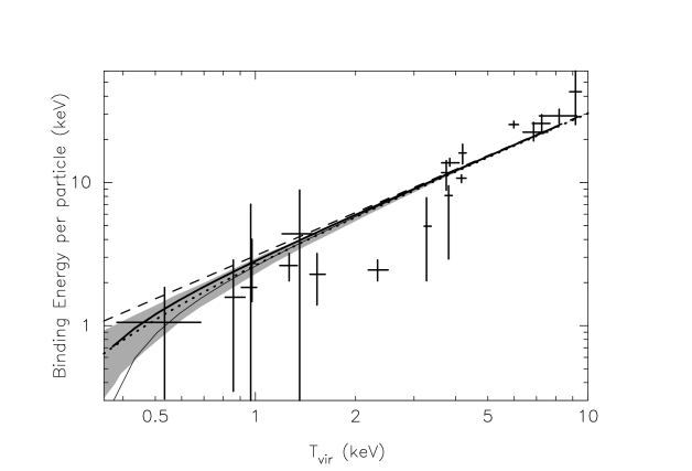
Figure 8: The prediction from our calculations is presented in the form of the final binding energy per particle of the central region of groups and clusters against the gas temperature. The data points are from the Figure 9 of Lloyd-Davies et al. (2000), and the dashed line refers to their fit $E\propto T$, derived from the data points for clusters with $T\geq 4$ keV. The dotted line refers to their second fit, with a constant excess energy of $0.44$ keV per particle (subtracted from the binding energy)along with a formal 1 $\sigma$ confidence interval shown by the shaded region. The thick solid line uses $f_{pdV}=3/8$ and the thin solid line uses $f_{pdV}$ from Figure 3.

The evolution of the rate of energy input (Figure 7) shows that the heat input before $z\sim 5$ is almost negligible. Most of the heating occurs in the range $z\sim 1\hbox{--}4$. It is also clearly seen that the ICM of poor groups is heated at lower redshifts, compared to the gas in massive clusters. This follows from the simple consideration that the evolution of objects in a given mass range (here, that of the quasars) typically occurs earlier in more massive clusters. Our results, therefore, suggests that the ICM in clusters were “preheated”, before the major mergers took place in them, whereas, the ICM in groups of galaxies were heated at epochs similar to that of their formation. It is interesting to note that the energy input epoch lies below the upper limit from recent observations of Lloyd-Davies et al. (2000). It is also consistent with the limit on the range of redshifts as shown by Yamada & Fujita (2001) given the level of uncertainty.

Recently, accelerated particles from shocks as a result of the formation of clusters have been hypothesized to be the source for the diffuse gamma ray background (Loeb & Waxman 2000). This gamma ray production will be suppressed, however, if the gas in the clusters were heated substantially at earlier epochs (Totani & Inoue 2001). Our results show that the ICM in massive clusters were preheated (and earlier than the ICM in groups), and the suppression of the gamma ray production will, therefore, be an important effect, if confirmed.

Finally, we discuss the uncertainties involved in our calculation. Apart from the uncertainties in cosmological parameters, the major uncertainties lies in the factors $f_{q}$ (§2) (connecting the abundances of quasars with PS mass function) , $f_{o}$ (the fraction of quasars with outflows) ,$f_{pdV}$ and $f_{gas}$. Among these, the most uncertain factor is $f_{o}$, which we have assumed to be of the order of unity for BAL outflows. The uncertainty in this factor will be reflected in the uncertainty of the final heat input (with a direct proportionality; see eqn 17). The uncertainty in $f_{pdV}$ has been already discussed earlier, and we found that even if $f_{pdV}$ is as low as $3/8$ for all cases, the final excess energy is certainly larger than that from supernovae driven winds, and is still within the required range of excess energy, especially for loose groups. As far as the uncertainty in $f_{gas}$ is concerned, we have also done our calculation with a varying $f_{gas}$, e.g., of the type,

$$f_{gas}=0.15(1+z)^{-0.5}\,(M_{cl}/10^{15}h^{-1})^{0.1}\,,$$ (24)

as has been advocated by Ettori & Fabian (1999), and we have found that the excess energy is approximately doubled in this case. It is, however, not clear if this correlation is a result of the excess energy, and, so, it would not be appropriate to attach much significance to this result. We have also varied the lower limit in our estimate of $f_{q}$ (eq. 1) and found that changing the lower limit from $10^{12}$ M_⊙ to $10^{11}$ M_⊙ increases the final heat input by only $\sim 10$ %. This is because of the fact that the increase in the number of quasars is compensated by the decrease in their mechanical luminosity. Lastly, we have already discussed in detail the uncertainty in the net formation rate of quasars in clusters, and as explained in §2, our approach here has been very conservative, and the final results should be regarded as conservative estimates in this regard.

6 Summary

We have calculated the excess energy deposited by quasar outflows in clusters in order to explain the observations of excess entropy in groups and clusters of galaxies. We summarise our findings below:

(1) We have used the extended Press-Sechter formalism to derive a formation rate of quasars inside clusters and groups, as a function of the cluster/group mass and its formation redshift.

(2) We have calculated the fraction of the kinetic luminosity of outflows (RLQ and BAL outflows) that is deposited onto the ambient medium, as a function of the density and temperature of the ambient medium. For outflows from radio-loud quasars, we have included the evolution of the cocoon after the jet turns off.

(3) The final excess energy from the mechanical work done by quasar outflows is found to be of order $0.18\hbox{--}0.85$ keV per particle, and is consistent with the data available at present. The excess energy in this scenario comes mainly from BAL outflows, with radio galaxies supplying about a tenth of the total. Keeping in mind the uncertainties in the estimate of energetics and abundances of radio and BAL outflows, we conclude that both radio galaxies and BAL outflows are promising candidates for heating the ICM. We found that this excess energy increases with decreasing mass of the cluster/group. This prediction could be tested with better data in the near future. The excess energy does not depend strongly on the formation redshift.

(4) The epoch of heating is found to be in the range $z\sim 1\hbox{--}4$, where this epoch is at lower redshifts for low mass clusters.

The authors would like to thank Nahum Arav, Andrew Blain, Sergio Colafrancesco, Zoltan Haiman, Subhbrata Majumdar and Trevor Ponman for valuable discussions. We have also benefitted from the detail comments of the anonymous referee. We are grateful to Ed Lloyd-Davies for supplying the data points for binding energy. We would also like to thank Rekhesh Mohan for help with plotting packages.

References

- [bn] Bahcall, J. N. & Chokshi, A. 1991, ApJ, 380, L9
- [bn] Balogh, M. L., Babul, A. & Patton, D. R. 1999, MNRAS, 307, 463
- [bn] Begelman, M. C. & Cioffi, D. F. 1989, ApJ, 345, L21
- [bn] Bialek, J. J., Evrard, A. E. & Mohr, J. 2001, ApJ, 555, 597
- [bn] Bicknell, G. V., Dopita, M. A. & O’Dea, C. P. O. 1997, ApJ, 485, 112
- [bn] Blain, A. W. & Longair, M. S. 1993, MNRAS, 265, L21
- [bn] Borgani, S., Governato, F., Wadsley, J., Menci, N., Tozzi, P., Lake, G., Quinn, T. & Stadel, J. 2001, ApJL, 559, L71
- [bn] Bower, R. G. 1991, MNRAS, 248, 332
- [bn] Brüggen, M. & Kaiser, C. R. 2001, MNRAS, 325, 676
- [bn] Bryan, G. L. & Norman, M. L. 1998, ApJ, 495, 80
- [bn] Cavaliere, A., Menci, N. & Tozzi, P. 1997, ApJ, 484, L21
- [bn] Chiu, W. A. & Ostriker, J. P. 2000, ApJ, 534, 507
- [bn] Churazov, E., Brüggen, M., Kaiser, C. R., Böhringer, H., Forman, W. 2001, ApJ, 554, 261
- [bn] David, L. P., Forman, W. & Jones, C. 1991, ApJ, 380, 39
- [bn] Daly, R. A. 1994, ApJ, 426, 38
- [bn] Eke, V., Navarro, J. F. & Frenk, C. S. 1998, ApJ, 503, 569
- [bn] Ellingson, E., Green R. F. & Yee, H. K. C. 1991, ApJ, 371, 49
- [bn] Elvis, M. et al. 1994, ApJS, 95, 1
- [bn] Ettori, S. & Fabian, A. C. 1999, MNRAS, 305, 834
- [bn] Evrard, A. E. & Henry, J. P. 1991, ApJ, 383, 95
- [bn] Fisher, K. B., Bahcall, J. N., Kirhakos, S., Schneider, D. P. 1996, ApJ, 468, 469
- [bn] Furlanetto, S. & Loeb, A. 2001, 556, 619 (FL01)
- [bn] Gallagher, S. C. et al. 1999, ApJ, 519, 549
- [bn] Gebhardt, K. et al. 2000, ApJ, 543, 5
- [bn] Gull, S. F. & Northover, K. J. E. 1973, Nature, 224, 80
- [bn] Haiman, Z. Loeb, A. 1998, ApJ, 503, 505
- [bn] Inoue, S. & Sasaki, S. 2001, ApJ, 562, 618
- [bn] Haehlent, M. & Rees, M. J. 1993, MNRAS, 263, 168
- [bn] Kaiser, N. 1991, ApJ, 383, 104
- [bn] Kaiser, C. R. & Alexander, P. 1999, MNRAS, 302, 515
- [bn] Kaiser, C. R. 2000, A&A, 362, 447
- [bn] Kitayama, T. & Suto, Y. 1996, ApJ, 469, 480
- [bn] Kravtsov, A. V. & Yepes, G. 2000, MNRAS, 318, 227
- [bn] Krolik, J. 1999, Active Galactic Nuclei (Princeton University Press: Princeton)
- [bn] Lacey, C. & Cole, S. 1993, MNRAS, 262, 627
- [bn] Lahav, O., Lilje, P. B., Primack, J. R., Rees, M. J. 1991, MNRAS, 251, 128
- [bn] Ledlow, M. J. & Owen, F. N. 1996, AJ, 112, 9
- [bn] Lloyd-Davies, E. J., Ponman, T. J. & Cannon, D. B. 2000, MNRAS, 315, 689
- [bn] Loeb, A. & Waxman, E. 2000, Nature, 405, 156
- [bn] Magorrian, J. et al. 1998, AJ, 115, 2285
- [bn] Mohr, J. J. & Evrard, A. E. 1997, ApJ, 491, 38
- [bn] Nath, B. B. 1995, MNRAS, 274, 208
- [bn] Navarro, J. F., Frenk, C. S. & White, S. D. M. 1995, MNRAS, 275, 720
- [bn] Percival, W. & Miller, L. 1999, MNRAS, 309, 823
- [bn] Ponman, T. J., Cannon, D, B. & Navarro, J. F. 1999, Nature, 397, 135
- [bn] Sasaki, S. 1994, PASJ, 46, 427
- [bn] Scheuer, P. A. G. 1982, in IAU Symp. 97, Extragalactic RAdio Sources, ed. D. S. Heeschen & C. M Wade (Dordrecht: Reidel), 163
- [bn] Schindler, S. 1999, A&A, 349, 435
- [bn] Stern, D. et al. 2000, AJ, 119, 1526
- [bn] Totani, T. & Inoue, S. 2002, Astroparticle Physics, 17, 79
- [bn] Valageas, P. & Silk, J. 1999, A&A, 350, 725
- [bn] Voit, G. M., Weymann, R. J. & Korista, K. T. 1993, ApJ, 413, 95
- [bn] Weymann, R. J., Morris, S. L., Foltz, C. B. & Hewett, P. C. 1991, ApJ, 373, 23
- [bn] Weymann, R. J. 1997, in Mass Ejection from AGN, ed. Arav, N., Shlosman, I. & Weymann, R. J. (ASP Press: San Fransisco), p.3
- [bn] Willot, C. J., Rawlings, S., Blundell, K. M. & Lacy, M. 1999, MNRAS, 309, 1017
- [bn] Wold, M., Lacy, M., Lilje, P. B., Serjeant, S., 2001, MNRAS, 323, 231
- [bn] Wu, K. K. S., Fabian, A. & Nulsen, P. E. J. 2000, MNRAS, 318, 889
- [bn] Yamada, M., Sugiyama, N. & Silk, J. 1999, ApJ, 622, 66
- [bn] Yamada, M. & Fujita, Y. 2001, ApJ, 553, L145