The counterrotating core and the black hole mass of IC 1459

Abstract

The E3 giant elliptical galaxy IC 1459 (catalog ) is the prototypical galaxy with a fast counterrotating stellar core. We obtained one HST/STIS long-slit spectrum along the major axis of this galaxy and CTIO spectra along five position angles. The signal-to-noise ($S/N$) of the ground-based data is such that also the higher order Gauss-Hermite moments ($h_{3}$–$h_{6}$) can be extracted reliably. We present self-consistent three-integral axisymmetric models of the stellar kinematics, obtained with Schwarzschild’s numerical orbit superposition method. The available data allow us to study the dynamics of the kinematically decoupled core (KDC) in IC 1459 and we find it consists of stars that are well-separated from the rest of the galaxy in phase space. In particular, our study indicates that the stars in the KDC counterrotate in a disk on orbits that are close to circular. We estimate that the KDC mass is $\approx 0.5$% of the total galaxy mass or $\approx 3\times 10^{9}M_{\odot}$.

We estimate the central black hole mass $M_{\bullet}$ of IC 1459 independently from both its stellar and its gaseous kinematics. Although both tracers rule out models without a central black hole, neither yields a particularly accurate determination of the black hole mass. The main problem for the stellar dynamical modeling is the fact that the modest $S/N$ of the STIS spectrum and the presence of strong gas emission lines preclude measuring the full line-of-sight velocity distribution (LOSVD) at HST resolution. The main problem for the gas dynamical modeling is that there is evidence that the gas motions are disturbed, possibly due to non-gravitational forces acting on the gas. These complications probably explain why we find rather discrepant BH masses with the different methods. The stellar kinematics suggest that $M_{\bullet}=(2.6\pm 1.1)\times 10^{9}M_{\odot}$ ($3\sigma$ error). The gas kinematics suggests that $M_{\bullet}\approx 3.5\times 10^{8}M_{\odot}$ if the gas is assumed to rotate at the circular velocity in a thin disk. If the observed velocity dispersion of the gas is assumed to be gravitational, then $M_{\bullet}$ could be as high as $\sim 1.0\times 10^{9}M_{\odot}$. These different estimates bracket the value $M_{\bullet}=(1.1\pm 0.3)\times 10^{9}M_{\odot}$ predicted by the $M_{\bullet}$-$\sigma$ relation. It will be an important goal for future studies to attempt comparisons of black hole mass determinations from stellar and gaseous kinematics for other galaxies. This will assess the reliability of black hole mass determinations with either technique. This is essential if one wants to interpret the correlation between the BH mass and other global galaxy parameters (e.g. velocity dispersion) and in particular the scatter in these correlations (believed to be only $\sim 0.3$ dex).

1 Introduction

The E3 giant elliptical galaxy IC 1459 ($M_{V}\simeq-22.3$ [LEDA, see Paturel et al. 1997], $D=30.3\pm 4.0$ Mpc [Ferrarese & Merritt 2000], $R_{e}\simeq 40\farcs 6$ [Burkert 1993]) is a member of a loose group consisting mainly of spirals. It shows clear signs of past interaction, evidenced by stellar “spiral arms” detected on deep photographs (Malin, 1985) and shells at large radii (Forbes & Reitzel, 1995). The nuclear region harbors a fast counterrotating stellar component (Franx & Illingworth, 1988), which cannot be identified as a separate structure in photometric observations. A blue LINER source (unresolved at HST resolution), surrounded by patchy dust absorption and by a gaseous disk, is found at the very center (Forbes, Franx, & Illingworth, 1995; Carollo et al., 1997; Verdoes Kleijn et al., 2000, hereafter VK00).

VK00 measured the mass of the central supermassive black hole in IC 1459 by analyzing kinematical observations of the nuclear gas disk, obtained with the Faint Object Spectrograph (FOS) on board the Hubble Space Telescope (HST). They found a central black hole mass of $M_{\bullet}=(2-6)\times 10^{8}M_{\odot}$ (scaling their values to our adopted distance). They also calculated isotropic two-integral axisymmetric dynamical models for ground-based major-axis stellar kinematics, resulting in a significantly larger mass estimate ($M_{\bullet}=[4-6]\times 10^{9}M_{\odot}$). For comparison, the $M_{\bullet}$-$\sigma$ relation (Ferrarese & Merritt, 2000; Gebhardt et al., 2000) as given by Tremaine et al. (2002) predicts a black hole mass of $(1.1\pm 0.3)\times 10^{9}M_{\odot}$.

In this paper, we construct axisymmetric three-integral models for IC 1459, using Schwarzschild’s orbit-superposition method (Rix et al., 1997; van der Marel et al., 1998; Cretton et al., 1999). The models are constrained by HST/STIS stellar kinematics measurements along the major axis and deep, ground-based spectroscopic observations along five different position angles of the slit. We show that this data-set allows us to derive information on the nature of the kinematically decoupled component (KDC). We also re-address the value for the mass of the nuclear BH in this galaxy.

This paper is organized as follows. We discuss the spectroscopic and photometric data in Section 2 and present the adopted dynamical model in Section 3. We discuss our results in Section 4 and summarize our conclusions in Section 5.

2 Data

2.1 HST spectroscopy

An HST spectrum of IC 1459 was obtained with STIS (GO 7352, PI: C.M. Carollo) along the galaxy major axis (as determined from the HST central isophotes), using the G430L grating with the 52″$\times$0$\farcs$1 slit. Four exposures, slightly shifted in the spatial direction, were obtained for a total of 9812 seconds. The availability of four shifted images allowed for a good removal of the numerous hot and bad pixels, together with cosmic rays, during the coaddition.

The extraction of the stellar kinematics was performed using the pixel-space Line-Of-Sight Velocity Distribution (LOSVD) fitting method of van der Marel (1994b). In pixel space, the masking of the prominent gas emission lines during the fit becomes straightforward. Specifically, a K3 III template star, observed with the 0$\farcs$2 STIS slit (GO 7388, PI: D. Richstone; no acceptable stellar template was available for the 0$\farcs$1 slit), was convolved with a parametrized LOSVD. The parameters of the LOSVD were optimized to the lowest $\chi^{2}$ by direct comparison with the observed spectrum. The galaxy spectrum was rebinned spatially before fitting, to an average S/N$\approx$20 per Å. The error images produced by the STScI pipeline were used to weight the measurements and estimate the errors in the fit. Our IDL fitting procedure differs from that of van der Marel (1994b) in the following aspects:

1. We used the elegant DIRECT deterministic global optimization algorithm (Jones, Perttunen, & Stuckman, 1993) to perform the $\chi^{2}$ optimization for the nonlinear variables $V$ and $\sigma$. This method is guaranteed to find the global minimum of a (possibly non-smooth) nonlinear function inside a finite box, even in the presence of multiple minima. It can be effectively used in many non-smooth real-world optimization problems with a small number of variables ($N\lesssim 10$).

2. We performed a $3\sigma$ clipped fit to make the fit stable against outliers (e.g. residual bad pixels, unmasked gas emission lines or template mismatch). In practice, once the global minimum is found, the galaxy pixels which deviate more than $3\sigma$ from the best fitting template spectrum are added to the list of masked pixels. The global optimization is repeated from scratch on the new set of pixels. This process is iterated until the set of bad pixels does not change anymore.

3. The errors on the $V$ and $\sigma$ fitting parameters are determined from the confidence levels for a $\chi^{2}$ distribution with two degrees of freedom.

The resulting dispersion measurements $\sigma_{\mathrm{fit}}$ were corrected by approximating the line-spread-function (LSF) by a Gaussian, for both the galaxy and the template star. The template was observed with an effective instrumental dispersion $\sigma_{{\rm LSF},t}\approx 100$ km s^-1 (Leitherer et al., 2001), while the galaxy was observed with $\sigma_{{\rm LSF},g}\approx 167$ km s^-1. The effective instrumental dispersion for the template star is smaller than that of the galaxy, even though the star was observed with a larger slit. The reason for this is that the STIS PSF falls completely within the 0$\farcs$2 slit that was used to observe the template, so that the template LSF is determined essentially by the PSF size. The corrected dispersion $\sigma$ was obtained from

$$\sigma^{2}=\sigma^{2}_{\rm fit}-\sigma^{2}_{{\rm LSF},g}+\sigma^{2}_{{\rm LSF},t}.$$ (1)

This correction is of the same order of magnitude as the measurement errors. No kinematic measurements could be extracted from the two central rows (0$\farcs$05 from the galaxy center) of the STIS spectrum due to the sharp decrease of the absorption line S/N of the stellar component, caused by the rise of a featureless non-thermal continuum from the central source. The non-thermal nature of the continuum is indicated by the sharp decrease of the line-strength parameter $\gamma$ towards the center.

The measured kinematical profiles are presented in Table 1 and in Figure 8.

Table 1: IC 1459, PA=34^∘, STIS stellar kinematics.

R	$V$	$\Delta V$	$\sigma$	$\Delta\sigma$
(″)	(km s-1)	(km s-1)	(km s-1)	(km s-1)
-1.50	-146	20	296	22
-1.03	-146	20	269	20
-0.73	-109	20	309	22
-0.48	-161	22	295	22
-0.25	-72	30	349	24
-0.10	-87	38	324	42
0.10	83	42	359	42
0.22	91	24	315	26
0.40	128	20	309	20
0.62	128	22	319	22
0.92	150	22	350	26
1.37	76	22	298	22

2.2 Ground-based spectroscopy

We also analyzed a set of ground-based spectroscopic observations taken with the CTIO 4m telescope in November 1988. These observations were made along five different position angles with a 1$\farcs$5 wide slit, using a CCD with a 0$\farcs$73 pixel size. The seeing PSF was $\approx 1\farcs 5$ FWHM during the observations. The major axis, two $\pm 45^{\circ}$ intermediate axes and two position angles close to the minor axis were observed. The location of the different slit positions is shown in Figure 1. The major axis data were presented previously in van der Marel & Franx (1993). The mean velocity $V$, the velocity dispersion $\sigma$ and the higher order Gauss-Hermite moments ($h_{3}$–$h_{6}$) were extracted from the high signal-to-noise spectra by the method described in that paper. The data are presented in Table 2.

Table 2: IC 1459, CTIO stellar kinematics and velocity profiles shape.

R	$V$	$\Delta V$	$\sigma$	$\Delta\sigma$	$h_{3}$	$\Delta h_{3}$	$h_{4}$	$\Delta h_{4}$	$h_{5}$	$\Delta h_{5}$	$h_{6}$	$\Delta h_{6}$
(″)	(km s-1)	(km s-1)	(km s-1)	(km s-1)
PA=39∘
-25.2	36.6	8.9	259.1	8.8	-0.008	0.031	-0.034	0.030	-0.017	0.033	0.077	0.031
-13.9	20.1	6.5	286.8	6.3	0.057	0.018	-0.027	0.019	-0.053	0.021	0.056	0.021
-7.3	-20.6	6.6	292.8	6.3	0.058	0.018	-0.003	0.019	-0.054	0.021	0.038	0.021
-4.7	-51.5	7.5	297.6	7.4	0.088	0.020	-0.009	0.021	-0.062	0.023	0.038	0.023
-3.7	-75.0	9.9	326.9	9.5	0.076	0.022	-0.019	0.023	-0.057	0.025	0.012	0.025
-2.9	-74.2	9.2	338.3	8.9	0.077	0.019	-0.006	0.020	-0.102	0.022	0.021	0.022
-2.2	-84.5	7.7	333.0	7.3	0.085	0.016	0.008	0.017	-0.062	0.019	0.023	0.019
-1.5	-85.5	6.5	339.9	6.5	0.079	0.014	0.016	0.014	-0.093	0.016	0.011	0.016
-0.7	-54.8	5.7	344.3	12.0	0.049	0.012	0.017	0.012	-0.087	0.013	0.021	0.013
0.0	-4.7	5.4	355.8	12.0	-0.030	0.011	-0.012	0.011	-0.041	0.013	0.033	0.012
0.7	58.0	5.6	342.6	12.0	-0.068	0.012	-0.041	0.012	0.003	0.014	0.068	0.014
1.5	79.9	6.5	332.3	6.2	-0.119	0.015	0.003	0.015	0.008	0.016	0.048	0.017
2.2	84.3	7.5	329.1	7.3	-0.158	0.017	-0.004	0.018	-0.006	0.020	0.029	0.020
2.9	80.7	9.1	339.9	9.1	-0.148	0.021	-0.013	0.021	0.032	0.023	0.082	0.024
3.7	75.7	10.0	333.2	9.4	-0.115	0.022	0.003	0.022	-0.034	0.025	-0.001	0.025
4.7	54.1	8.2	319.2	7.7	-0.081	0.019	-0.036	0.020	-0.015	0.022	0.074	0.023
7.3	26.7	6.6	303.9	6.1	-0.072	0.017	-0.045	0.018	0.017	0.020	0.080	0.020
13.9	-12.9	6.4	283.3	5.9	0.009	0.018	-0.044	0.019	0.002	0.021	0.057	0.020
25.2	-38.7	8.8	255.5	8.8	0.050	0.030	-0.037	0.030	-0.058	0.033	0.045	0.031
PA=83∘
-25.2	18.3	10.4	238.1	10.7	-0.064	0.041	-0.013	0.038	-0.016	0.042	0.054	0.040
-13.9	10.9	7.4	273.2	6.9	-0.027	0.022	-0.019	0.023	-0.002	0.025	0.044	0.024
-7.3	-9.9	7.0	268.0	7.0	0.051	0.022	0.036	0.022	-0.060	0.025	-0.004	0.024
-4.7	-31.5	7.6	272.9	7.7	0.028	0.024	0.028	0.025	-0.034	0.027	0.016	0.026
-3.7	-38.3	10.3	300.6	10.3	0.068	0.026	0.066	0.028	-0.046	0.031	-0.051	0.031
-2.9	-41.3	8.7	304.9	8.5	0.065	0.022	0.042	0.023	-0.029	0.026	-0.003	0.026
-2.2	-44.4	7.8	317.4	7.4	0.062	0.018	-0.011	0.019	-0.078	0.021	0.013	0.021
-1.5	-50.8	6.6	336.7	6.6	0.079	0.014	0.007	0.015	-0.083	0.016	0.010	0.016
-0.7	-32.4	6.2	370.2	12.0	0.027	0.012	0.006	0.012	-0.063	0.013	0.019	0.013
0.0	4.7	6.0	370.0	12.0	-0.036	0.011	-0.006	0.011	-0.061	0.013	0.027	0.012
0.7	45.9	6.1	347.7	12.0	-0.053	0.013	-0.024	0.013	-0.015	0.014	0.055	0.014
1.5	53.1	6.9	338.6	6.7	-0.049	0.015	0.004	0.015	0.017	0.017	0.026	0.017
2.2	48.4	8.0	325.7	8.0	-0.074	0.018	0.006	0.019	-0.031	0.021	0.024	0.022
2.9	31.1	8.8	308.7	8.7	-0.064	0.022	-0.007	0.023	-0.033	0.026	0.053	0.026
3.7	17.7	10.6	309.4	10.2	-0.066	0.026	-0.016	0.028	-0.032	0.030	0.054	0.031
4.7	14.3	8.3	295.6	8.2	-0.017	0.022	-0.005	0.023	-0.028	0.026	0.049	0.026
7.3	-7.8	7.1	279.6	7.0	-0.034	0.021	-0.005	0.022	-0.028	0.024	0.034	0.023
13.9	-37.8	6.8	260.7	6.8	0.034	0.023	0.015	0.023	-0.053	0.025	0.011	0.024
25.2	-56.4	10.6	273.3	10.3	0.041	0.032	-0.027	0.033	-0.054	0.037	0.066	0.036
PA=120∘
-25.2	11.0	12.2	257.8	11.7	0.034	0.040	-0.069	0.040	0.028	0.045	0.077	0.042
-13.9	23.0	7.4	248.8	7.6	0.053	0.026	0.014	0.026	-0.012	0.029	-0.009	0.027
-7.3	5.0	6.9	259.3	7.1	0.031	0.023	0.031	0.023	-0.014	0.026	0.007	0.024
-4.7	13.2	9.1	294.9	9.0	0.052	0.024	0.058	0.026	-0.073	0.029	-0.036	0.028
-3.6	7.6	11.1	311.5	10.6	0.008	0.026	-0.001	0.028	-0.045	0.031	0.009	0.031
-2.9	-9.7	9.4	294.8	9.2	0.036	0.025	0.042	0.026	-0.090	0.029	0.002	0.029
-2.2	-2.9	7.8	294.8	7.5	0.053	0.020	0.021	0.022	-0.061	0.024	0.011	0.024
-1.5	2.2	6.8	322.2	6.3	-0.007	0.015	0.001	0.016	-0.035	0.018	0.001	0.018
-0.7	-10.0	5.9	359.3	12.0	-0.013	0.012	0.002	0.012	-0.033	0.014	0.004	0.013
0.0	-3.8	5.9	380.0	12.0	-0.001	0.011	-0.015	0.011	-0.034	0.012	0.023	0.012
0.7	17.1	6.3	363.4	12.0	-0.011	0.012	-0.006	0.012	-0.022	0.014	0.035	0.013
1.5	1.3	6.7	331.5	6.8	-0.011	0.015	0.017	0.016	-0.025	0.018	0.014	0.018
2.2	-1.5	8.1	310.3	7.9	0.029	0.019	0.007	0.021	-0.030	0.023	0.046	0.023
2.9	-4.9	9.5	299.3	9.6	0.011	0.024	0.050	0.026	-0.036	0.029	0.001	0.029
3.6	-4.5	10.7	291.1	10.4	-0.006	0.028	0.021	0.030	-0.024	0.034	-0.002	0.033
4.7	-4.8	8.6	288.8	8.4	0.008	0.023	-0.025	0.025	0.012	0.028	0.049	0.027
7.3	-1.9	6.9	262.8	7.1	-0.012	0.023	0.035	0.023	0.003	0.026	0.006	0.025
13.9	-15.9	7.6	257.8	7.9	-0.023	0.026	-0.001	0.026	0.040	0.029	0.062	0.028
25.2	-26.0	10.9	217.3	11.7	0.087	0.047	0.027	0.044	0.016	0.049	-0.026	0.048
PA=128∘
-25.2	5.6	11.6	242.5	11.7	-0.006	0.044	-0.046	0.042	0.012	0.047	0.118	0.045
-13.9	10.6	7.2	247.3	7.5	0.030	0.027	0.003	0.026	0.007	0.029	0.044	0.027
-7.3	4.1	7.1	266.9	7.0	0.010	0.022	-0.006	0.023	-0.059	0.025	0.015	0.024
-4.7	6.1	8.2	277.9	8.2	-0.060	0.024	0.012	0.025	-0.049	0.028	0.011	0.027
-3.6	-4.1	10.1	284.7	9.8	0.011	0.029	0.023	0.030	-0.031	0.033	0.018	0.033
-2.9	-0.0	8.7	291.3	8.2	-0.028	0.023	-0.034	0.025	-0.080	0.027	0.053	0.027
-2.2	25.2	8.6	327.7	8.3	-0.028	0.019	-0.016	0.020	-0.056	0.022	0.036	0.023
-1.5	-2.3	7.5	351.2	7.1	-0.015	0.015	-0.007	0.015	-0.028	0.017	0.033	0.017
-0.7	-0.4	6.2	365.1	12.0	-0.013	0.012	-0.023	0.012	-0.038	0.014	0.036	0.013
0.0	-1.3	6.1	371.4	12.0	-0.027	0.011	-0.022	0.011	-0.057	0.013	0.052	0.012
0.7	-10.8	6.2	356.8	12.0	-0.013	0.013	-0.028	0.013	-0.045	0.014	0.070	0.014
1.5	-1.8	6.9	333.4	6.7	0.002	0.015	-0.004	0.016	-0.040	0.018	0.030	0.018
2.2	-9.2	8.3	319.5	8.1	0.002	0.019	0.011	0.020	-0.036	0.022	0.028	0.023
2.9	-7.4	9.3	312.2	9.1	0.001	0.023	0.016	0.024	-0.061	0.027	0.020	0.027
3.6	1.5	10.7	296.3	10.7	-0.008	0.028	-0.009	0.030	-0.080	0.033	0.051	0.033
4.7	5.0	8.6	289.5	8.5	0.008	0.024	0.019	0.025	-0.128	0.028	0.010	0.027
7.3	-10.4	6.6	248.6	6.4	0.027	0.023	-0.021	0.022	-0.059	0.025	0.033	0.024
13.9	-19.3	7.1	248.9	7.4	-0.002	0.026	0.011	0.025	-0.022	0.028	0.031	0.027
25.2	-29.1	11.9	245.1	11.2	0.065	0.040	-0.030	0.039	-0.010	0.044	-0.025	0.041
PA=173∘
-25.2	-45.5	10.5	229.5	10.9	0.046	0.042	0.003	0.040	0.004	0.044	0.039	0.043
-13.9	0.1	6.8	250.6	6.6	0.017	0.024	-0.031	0.023	-0.004	0.026	0.058	0.025
-7.3	5.0	7.3	290.0	7.2	-0.029	0.020	0.012	0.021	0.006	0.024	0.037	0.023
-4.7	33.6	7.6	275.7	7.5	-0.072	0.023	-0.012	0.023	-0.028	0.026	0.034	0.025
-3.7	47.9	9.7	308.7	9.4	-0.088	0.024	-0.006	0.026	0.040	0.028	0.041	0.029
-2.9	59.0	8.8	311.4	8.4	-0.089	0.022	-0.017	0.023	0.009	0.025	0.045	0.026
-2.2	57.7	8.0	329.5	7.8	-0.063	0.018	-0.007	0.019	0.001	0.021	0.039	0.021
-1.5	67.4	6.7	336.3	6.8	-0.063	0.015	0.013	0.015	-0.014	0.017	0.025	0.017
-0.7	41.3	6.0	349.1	12.0	-0.060	0.012	-0.024	0.012	-0.021	0.014	0.053	0.014
0.0	-3.9	5.8	357.8	12.0	-0.022	0.011	-0.019	0.011	-0.017	0.013	0.037	0.013
0.7	-40.4	5.7	344.5	12.0	0.006	0.012	-0.001	0.012	-0.045	0.014	0.024	0.014
1.5	-61.3	6.7	336.2	6.6	0.046	0.014	0.003	0.015	-0.066	0.016	0.005	0.016
2.2	-61.9	7.9	321.1	7.6	0.067	0.017	0.032	0.018	-0.033	0.021	-0.004	0.021
2.9	-71.9	8.2	299.5	8.2	0.054	0.021	0.006	0.022	-0.014	0.025	0.027	0.025
3.7	-34.2	10.4	314.4	10.0	0.003	0.024	0.027	0.026	-0.030	0.029	0.004	0.029
4.7	-25.4	9.1	312.5	9.0	0.006	0.022	0.042	0.023	-0.062	0.026	-0.006	0.026
7.3	-9.1	7.0	286.3	7.1	-0.002	0.020	0.021	0.021	-0.035	0.023	0.023	0.022
13.9	12.8	7.1	265.9	7.6	0.003	0.023	0.050	0.024	0.007	0.026	-0.013	0.025
25.2	19.0	10.3	250.5	10.2	-0.033	0.037	-0.023	0.036	0.111	0.040	0.020	0.038

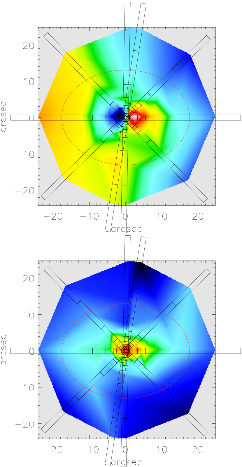
Figure 1: Interpolated velocity field of IC 1459. Upper Panel: mean velocity field, obtained by linear interpolation from the measured values at the aperture positions. The central counterrotating component is clearly visible. A representative galaxy isophote, the five slit positions and the regions along the slits that were averaged are also shown. Lower Panel: same as in the upper panel for the observed velocity dispersion field.

2.3 HST imaging: correction of dust absorption

For our dynamical modeling, we need to derive an $I$-band surface density model from the available WFPC2/F814W (460 s) Hubble Space Telescope image of IC 1459. A complication is that this galaxy contains gas and dust in its central regions, which has to be corrected for in order to obtain an accurate determination of the central stellar surface brightness. We derive this correction in a manner that is similar to Carollo et al. (1997, hereafter C97) and assume

1. the intrinsic color of the galaxy pixels that are affected by dust is the same as that of the surrounding pixels;

2. the dust is a screen in front of the stellar emission;

3. the Galactic extinction law (Cardelli, Clayton, & Mathis, 1989) applies.

In this process, we use the available WFPC2/F555W (1000 s) frame in addition to the WFPC2/F814W image.

In practice, C97 corrected the pixel values by assuming that all pixels on the same isophote have the same intrinsic color. We add the assumption that the intrinsic galaxy color varies smoothly as a function of radius. Specifically here we assume the color varies linearly with the logarithm of the radius. This assumption is justified by Figure 2. The pixel correction then involves the following steps:

1. We measure the average ellipticity and position angle on the original galaxy image.

2. We construct a calibrated color map (in our case $V-I$).

3. We perform a straight line fit to the pixel colors as a function of $\log m$, where $m$ represents the semimajor axis length (see Figure 2). The fit is done by minimizing the absolute deviation to reduce the effect of large systematic pixel value deviations due to dust.

4. We compute an $E(V-I)$ map by calculating, for every pixel, the color predicted from the previously fitted relation and subsequently subtracting this from the pixel value. The result is shown in Figure 3.

5. We correct the pixels above a given $E(V-I)$ threshold (in general as a function of $m$), using the standard Galactic extinction curve.

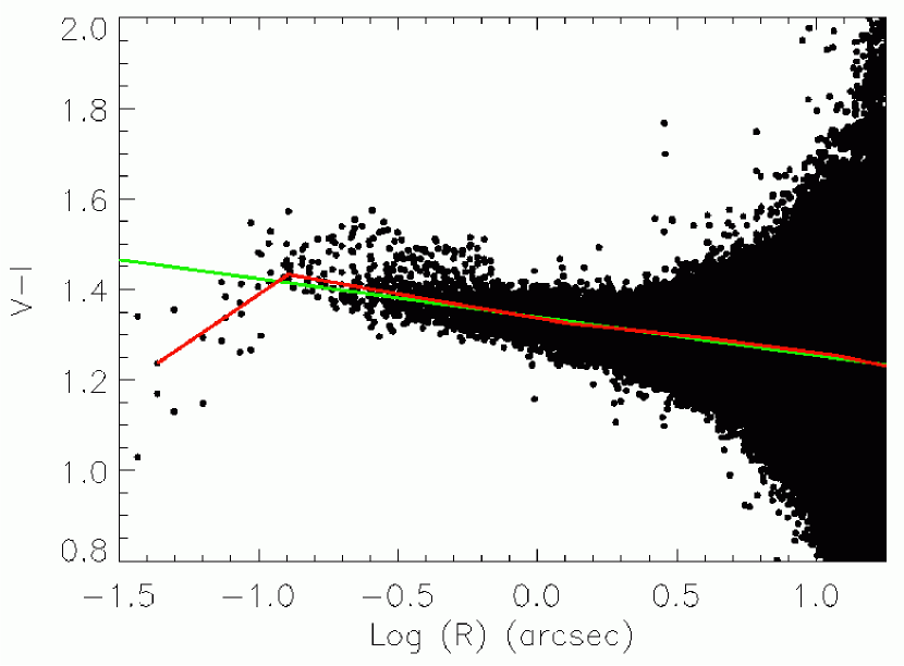
Figure 2: The calibrated $V-I$ color of every pixel in the WFPC2/PC1 image of IC 1459 as a function of its elliptical radius. The best-fitting straight line, obtained by minimizing the absolute deviation, is shown in green. For comparison, the red line shows the median color in logarithmically spaced radial bins. Notice the reddened pixels inside $R\lesssim 1\arcsec$, caused by dust effects, and the sharp decrease of the color in the nucleus $R\lesssim 0\farcs 1$, due to a blue source detected previously by Forbes et al. (1995) and C97.

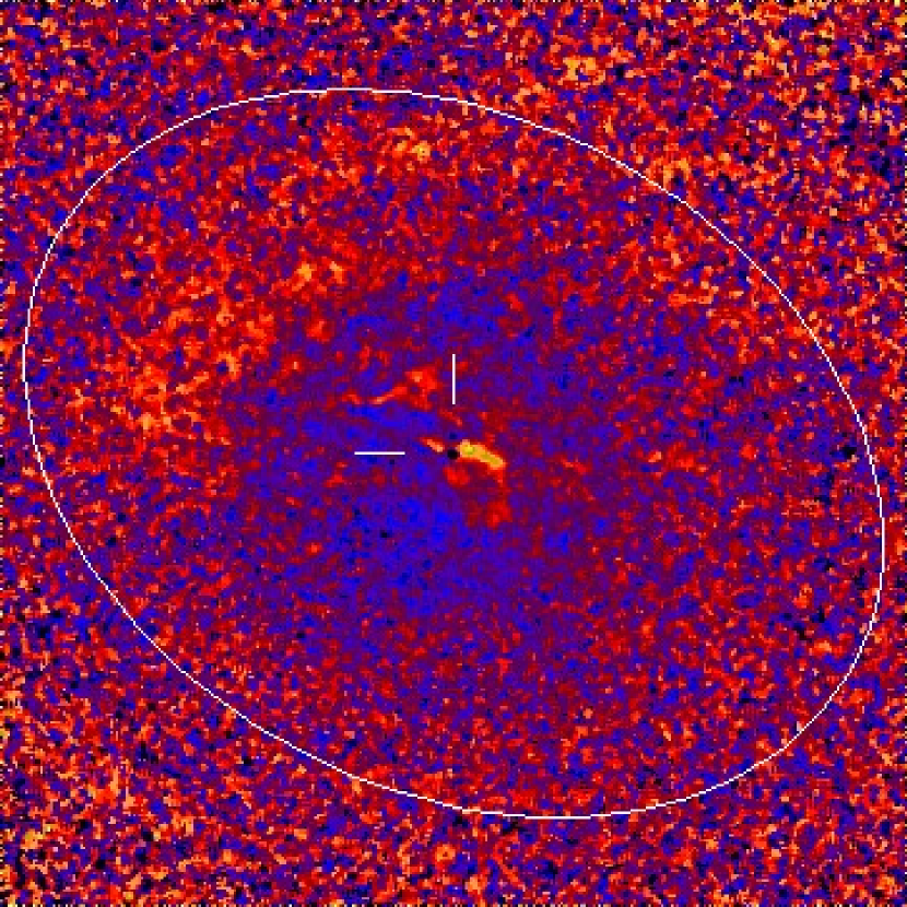
Figure 3: $E(V-I)$ map for the central regions of IC 1459, obtained after subtracting the underlying stellar color gradient (see text). Bright colors correspond to large color excesses. Notice the blue central spike (the black dot indicated by the two lines) surrounded by heavy dust absorption (jellow). A representative galaxy isophote, with an 8″ semi-major axis, is also shown.

This ad hoc method corrects the major effects of patchy dust absorption and can also be used to measure dust corrected color gradients (compare Figure 2 with Figure 1o in C97).

3 Dynamical model

3.1 The mass model with MGE

IC 1459 is not a perfectly axisymmetric body, evidenced by a small $\approx 5^{\circ}$ isophotal major axis twist in the range 25″–100″ (Franx et al. 1989; C97). Nevertheless, assuming axisymmetry seems reasonable to study its nuclear dynamics, given that our kinematical observations are all located inside the region that can be well reproduced by assuming axisymmetry.

The first step in the dynamical modeling is to obtain a parametrization of the stellar surface density. For this we adopted the Multi-Gaussian Expansion (MGE) method (Monnet, Bacon, & Emsellem, 1992; Emsellem, Monnet, & Bacon, 1994), which allows for non-elliptical isophotes and radial ellipticity variations.

We obtained an MGE fit to the WFPC2/F814W dust-corrected images of IC 1459 using the method and software developed by Cappellari (2002). The MGE fit was performed using both the PC1 (at full resolution) and the entire WFPC2 mosaic simultaneously. The PSF was parametrized by fitting a circular MGE model, of the form $PSF(R^{\prime})=\sum_{k=1}^{M}G_{k}\exp{[-R^{\prime 2}/(2\sigma^{\star 2}_{k})]}/(2\pi\sigma^{\star 2}_{k})$, to a PSF computed with TinyTim (Krist & Hook, 2001) for the center of the PC1 CCD. The numerical values of the relative weights $G_{k}$ (normalized such that $\sum_{k=1}^{M}G_{k}=1$), and of the dispersions $\sigma^{\star}_{k}$ are given in Table 3.

Figure 4 shows a comparison between the observed photometry and the MGE model along a number of profiles, while Table 4 gives the corresponding numerical values of the analytically deconvolved MGE parametrization of the galaxy surface brightness

$$\Sigma(x^{\prime},y^{\prime})=\sum_{j=1}^{N}\frac{L_{j}}{2\pi\sigma_{j}^{2}q^{\prime}_{j}}\exp\left[-\frac{1}{2\sigma_{j}^{2}}\left(x^{\prime 2}+\frac{y^{\prime 2}}{q^{\prime 2}_{j}}\right)\right].$$ (2)

Also tabulated are the distance-independent central surface brightness of each Gaussian $I^{\prime}_{j}=L_{j}/(2\pi\sigma_{j}^{2}q^{\prime}_{j})$. The central Gaussian (no. 1) represents the contribution of the blue unresolved central spike, which is of non-thermal origin and will not be included in the dynamical model calculation. The comparison between the isophotes of the convolved model and the actual image is shown in Figure 5. We confirm the finding of C97 that there is no photometric evidence for a nuclear disk in the dust corrected images.

Figure 4: Left Panels: Comparison between the WFPC2/F814W photometry of IC 1459 in counts (open squares) and the corresponding MGE best fit model (solid line) as a function of radius $R$. The individual convolved Gaussian components are also shown. The fit was performed along 19 sectors, each $5^{\circ}$ wide, linearly spaced in radius between the major and minor axis. Only every third sector is shown here. Right Panels: radial variation of the relative error $\epsilon$ along the profiles. Apart from the very innermost pixels where statistical fluctuations are important, the profiles are reproduced to within 2%. The RMS error is about 1.0%.

Table 3: Parameters of the HST/WFPC2/F814W circular MGE PSF

$k$	$G_{k}$	$\sigma_{k}^{\star}$
		(arcsec)
1	0.294	0.0224
2	0.559	0.0655
3	0.0813	0.214
4	0.0657	0.610

Table 4: MGE parameters for the deconvolved I-band WFPC2 surface brightness of IC 1459

$j$	$I^{\prime}_{j}$	$\sigma_{j}$	$q^{\prime}_{j}$	$L_{j}$
	(L⊙,I pc-2)	(arcsec)		($10^{9}$ L⊙,I)
1	727874	0.0172	1.000	0.0295
2	18191	0.268	0.899	0.159
3	22306	0.618	0.672	0.777
4	11511	0.993	0.815	1.25
5	11226	2.09	0.681	4.55
6	5243.0	3.77	0.775	7.82
7	1577.4	6.82	0.714	7.10
8	1105.6	11.2	0.738	13.9
9	337.28	21.8	0.732	15.9
10	194.31	39.6	0.733	30.3
11	59.276	126	0.774	99.5

Figure 5: Contour maps of the dust-corrected WFPC2 $I$-band image of IC 1459 at two different scales. Top Panel: the $35\arcsec\times 35\arcsec$ PC1 CCD. Bottom Panel: the entire $160\arcsec\times 160\arcsec$ WFPC2 mosaic. Superposed on the two plots are the contours of the MGE surface brightness model, convolved with the WFPC2 PSF. The model and data deviate more at larger radii, since the isophotal twist that occurs at these radii cannot be reproduced by an axisymmetric model.

3.2 Three-integral models

We model IC 1459 by using an axisymmetric three-integral implementation of Schwarzschild’s (1979) orbit superposition method, developed by Rix et al. (1997); van der Marel et al. (1998); Cretton et al. (1999) and Richstone et al. (2002). The method is described extensively in the above references and we will not repeat the details here. Very briefly, the stellar density is derived by deprojecting (see Appendix A) an MGE parametrization of the observed surface density (equation [2]), assuming axisymmetry and a value for the stellar mass-to-light ratio $\Upsilon$. Stellar orbits are integrated in the potential that is generated by both the stellar density and a central supermassive BH. Each orbit is projected onto the space of the observables, taking into account PSF convolution and aperture binning. Finally, the distribution of orbital weights that best fits both the luminosity density distribution of the model and the observed kinematics is determined by solving a Non-Negative Least-Squares (NNLS, Lawson & Hanson 1974) problem.

We modified the software implementation by van der Marel et al. (1998, hereafter M98) such that it can deal with the MGE parametrization of the surface brightness derived in the previous paragraph, in a way that is similar to Cretton & van den Bosch (1999). The differences between our software and the implementation used by M98 are:

1. Simplified calculation of the potential. This is possible because of the MGE formalism and the details described in Appendix A;

2. Substitution of the numerical integration of the luminosity density along the line of sight with the analytic MGE projection;

3. Simplified and more accurate (due to the smaller number of numerical integrations involved) evaluation of the density integration on a polar or Cartesian grid (Appendix B).

3.3 Orbit library

To include a representative set of orbits in the orbit library, we sample them on a grid that covers the full extent of the integral space $(E,L_{z},I_{3})$, where $E$ is the energy, $L_{z}$ is the angular momentum along the $z$ symmetry axis and $I_{3}$ is a non-classical integral. This is achieved by sampling the energy logarithmically in the radius of the circular orbit with the given energy $E(R_{c})$, from 0$\farcs$05 to 300″. This grid includes 99% of the total luminous mass of the galaxy. The quantity $\eta\equiv L_{z}/L_{\rm max}$ is sampled linearly on an open grid in the interval $[0,1]$. $I_{3}$ is sampled linearly in the angle $w$ on an open grid in the interval $[0,w_{\rm th}]$, where $w_{\rm th}$ is the angle $w$ for the “thin tube” orbit at the given $(E,L_{z})$ (see Figure 5 in M98 for details). After some testing we chose a $20\times 14\times 7$ grid in integral space (including both positive and negative $L_{z}$), but similar results (with longer computation times) were obtained with a $25\times 26\times 13$ grid. This choice of parameters is similar to that used in the modeling of other nearby galaxies (e.g. van der Marel et al. 1998; Verolme et al. 2002).

4 Results

4.1 Stellar kinematics

Our model has three free parameters: the galaxy inclination $i$, the BH mass $M_{\bullet}$ and the stellar mass-to-light ratio $\Upsilon$. Inclinations smaller than $i\lesssim 55^{\circ}$ can be excluded based on the observed axial ratio of IC 1459, since these values correspond to intrinsic stellar densities that are too flat for an elliptical galaxy.

We fitted dynamical models to the $V$, $\sigma$ and $h_{3}$–$h_{6}$ observations along all five position angles and to the STIS/G430L $V$ and $\sigma$ measurements. We varied the parameters $\Upsilon$ and $M_{\bullet}$ for three different values of the inclination $i=60^{\circ}$, $i=75^{\circ}$ and $i=90^{\circ}$. The overall best fit was found for an inclination $i=90^{\circ}$ (corresponding to edge-on viewing). Contours of equal $\chi^{2}$, using the confidence levels for a $\chi^{2}$-distribution with three degrees of freedom, are shown in the upper panel of Figure 6. The best-fit parameters are a mass-to-light ratio of $\Upsilon=3.1\pm 0.4$ (in the $I$-band) and a central black hole mass of $M_{\bullet}=(2.6\pm 1.1)\times 10^{9}M_{\odot}$ (3$\sigma$ level). The inclination is not strongly constrained by our data and our results do not depend significantly on the adopted value. In particular, the best-fitting black hole mass at $i=60^{\circ}$ is $M_{\bullet}=(2.5\pm 1.2)\times 10^{9}M_{\odot}$. The best-fit model has $\chi^{2}\approx 867$ with $N=594$ kinematical constraints. The fact that $\chi^{2}>N$ even for the best model, is due to some small systematic errors, which are in particular visible for the even Gauss-Hermite moments $h_{4}$ and $h_{6}$. The excellent match (Figure 7, 8) to the observed kinematical constraints along all position angles suggests that the decoupled core in IC 1459 can be well described as an axisymmetric component. This allows us to study its internal dynamics, shape and mass distribution.

Figure 6: Top Panel: Contours of constant $\chi^{2}$, measuring the goodness of fit of the edge-on axisymmetric models for IC 1459. The abscissa is the mass $M_{\bullet}$ of a point mass representing a nuclear BH; the ordinate is the constant stellar mass-to-light ratio $\Upsilon$. These two parameters uniquely determine the potential given the inclination $i$. Every dot corresponds to a three-integral axisymmetric dynamical model. The contours were obtained through a minimum curvature interpolation. The first three contours define the formal 68.3%, 95.4% and (heavy contours) 99.73% confidence regions for the three parameters $(i,M_{\bullet},\Upsilon)$ jointly; subsequent contours are characterized by a factor of 2 increase in $\Delta\chi^{2}$. The best fit is obtained with a mass for the BH $M_{\bullet}\simeq 2.6\times 10^{9}M_{\odot}$ and a stellar $\Upsilon\simeq 3.1$ in the $I$-band. Bottom Panel: Same as in top panel for a model with $\Upsilon$ varying as a function of radius (see text for details). Here the ordinate represents the value of $\Upsilon$ at a radius $R=1\arcsec$.

Figure 7: Data-model comparison. From top to bottom: the mean velocity $V$, the velocity dispersion $\sigma$ and the higher order Gauss-Hermite moments ($h_{3}-h_{6}$) as a function of position along the slit. From left to right: the measurements along the major (PA=39^∘), minor (PA=128^∘, 120^∘) and intermediate axis (PA=83^∘, 173^∘). The filled circles with error bars represent the measurements, while the solid line gives the prediction of the best fitting unregularized dynamical model, taking into account seeing and pixel binning. The dashed line shows the prediction of the high-regularization solution ($\Delta=1$). The case of small regularization ($\Delta=4$) lies between the two curves.

Figure 8: The fit to the STIS/G430L kinematic observations for the same model that is shown in Figure 7. The upper panel displays the mean velocity $V$, while the bottom panel is the velocity dispersion $\sigma$, both as a function of radius along the major axis. The filled circles with error bars represent the measurements, while the solid line gives the prediction of the best fit unregularized dynamical model. The dashed line shows the predictions of the high regularization solution ($\Delta=1$). As in Figure 7, the case of small regularization ($\Delta=4$) lies between the two curves.

The solid lines in Figure 7 and 8 were calculated by fitting to only the photometry and kinematics. The kinematical constraints are distributed over 95 apertures (not all independent), each of which provides 6 Gauss-Hermite moments and 12 STIS apertures with $V$ and $\sigma$ measurements. Selfconsistency is ensured by fitting to the mass in the meridional (120 constraints) and projected plane (140 constraints), as well as to the mass fractions contained in the kinematical apertures. The models therefore have to satisfy a total of 961 constraints, which are to some extent correlated. Since our library contains $20\times 14\times 7=1960$ orbits whose orbital weights are the unknowns that have to be determined, there is no unique solution that defines the internal dynamics of this galaxy (in the approximation of this model). In fact, the NNLS matrix equation that is solved is numerically rather ill-conditioned, giving rise to a distribution function composed of sharp isolated peaks. Such DFs are unphysical. A smoother and better (see Cretton et al. 1999; Verolme & de Zeeuw 2002) solution can be obtained by using regularization. The regularization scheme that is used here minimizes, up to a certain degree, the differences in weights between neighboring orbits. Although these additional regularization constraints result in a slightly poorer fit to the data, a considerable amount of smoothing can be forced upon the solution before systematic deviations in the fit become apparent.

Figure 9 shows the integral space [the weights on the $(E,L_{z},I_{3})$ grid] of our best-fitting model, for a selected set of energies (corresponding to the radii effectively constrained by the observations). The top row shows the integral space for the unsmoothed solution which, as a consequence, appears very noisy. A small amount of regularization ($\Delta=4$; see M98 for details) was added as a constraint in the middle row. While the fit to the data remains essentially unchanged, some coherent structures clearly emerge in the solution space. The bulk of the galaxy rotation can be recognized as a large bright (high weight) region at low and negative $\eta\equiv L_{z}/L_{\rm max}$ and high $w$ on the range $\approx$1″–13″. At radii smaller than $\approx$0$\farcs$8, the regularized solution contains a well-separated group of nearly circular orbits ($\eta\approx 1$), which counterrotates with respect to the main galaxy body. These orbits appear necessary to explain the observed rapid counterrotation in the kinematics. The contribution of the counterrotating component seems to decrease inside $R\lesssim 0\farcs 2$. This is probably not a real effect: there is not enough data inside this radius to constrain the phase space in detail and its appearance is dictated by the smoothness constraint.

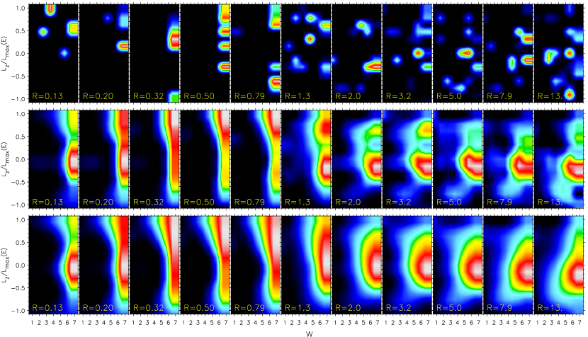
Figure 9: The top row shows the $(\eta,w)$ integral space (defined as described in the text) at a selected set of energies, for the best-fitting non-smooth orbit-superposition model. The radius of the circular orbit (in arcsec) at any given energy is printed at the bottom of each panel and only the radii that are actually constrained by the observed data are shown. The plots were obtained by bilinear interpolation on a $14\times 7$ grid in $(\eta,w)$, where each $(\eta,w)$ represents an orbit. Given that the value of $w$ does not have direct physical significance we labeled the abscissa with the bin number from 1–7. The colors show the fractional mass that was assigned to the orbit by the NNLS fit (bright colors correspond to large weights). The weights are normalized to the maximum value at the corresponding energy. Smoother solutions are obtained by adding regularization constraints to the NNLS fit. The second and third rows show the integral space for the same model with a small ($\Delta=4$) and a large ($\Delta=1$) amount of regularization, respectively. Negative values of $\eta\equiv L_{z}/L_{\rm max}(E)$ correspond to the bulk rotation of the galaxy body. The counterrotating component is clearly recognizable as a well-separated peak at $\eta\approx 1$ in the central and bottom row, in particular in the radial range 0$\farcs$3–0$\farcs$8 (panels 3–5 from the left).

The structure of integral space remains qualitatively the same at high regularization ($\Delta=1$, bottom row). This latter model is still able to produce a reasonable fit to all constraints (see dashed line in Figure 7, 8). Although our conclusions do not depend strongly on the regularization parameter $\Delta$, in the following we adopt $\Delta=4$ for our plots. Both Cretton et al. (1999) and Verolme et al. (2002) have carried out a number of tests of the Schwazrschild code, and established which value of $\Delta$ gives the best reconstruction of a known distribution function. The result is a $\Delta\sim 4$. Detailed comparison with independent results obtained by Gebhardt with a maximum entropy technique (which starts at the opposite end with a fully smooth distribution function, and then makes it less and less so) shows that again an amount of smoothing equivalent to our $\Delta\sim 4$ is optimal.

Both the best fit values and the details of the internal kinematic structure are in excellent agreement with our previous results (Cappellari, 2000; Cappellari et al., 2001), which started from a triple power-law parametrization of the stellar surface density instead of the MGE expansion and were constrained by ground-based data only. This comparison shows that the best-fitting parameters do not depend on the details of the adopted stellar density parametrization. However, our best-fitting black hole mass is slightly larger than the value $(1.1\pm 0.3)\times 10^{9}M_{\odot}$ that is predicted by the $M_{\bullet}$-$\sigma$ relation (Ferrarese & Merritt, 2000; Gebhardt et al., 2000) as given by Tremaine et al. (2002).

The contribution of a dark halo becomes evident in the observed stellar kinematics only well beyond an effective radius, and hence can be safely ignored (Carollo et al. 1995; Gerhard et al. 2001). Furthermore, we follow standard practice and assume that the stellar mass-to-light ratio does not vary with radius. To determine whether our results depend on this assumption, we also ran models in which $\Upsilon$ follows the change of the $V-I$ color presented in Fig. 2. The color gradient of IC 1459 is $d(V-I)/d(\log R)\approx-0.084$. Using models from Charlot, Worthey & Bressan (1996), the color variation can be translated into a fractional decrease of $\Upsilon$ by $\sim 15$ per cent per decade in radius, more or less independent of whether the color gradient is due to age or to metallicity variations. The results obtained from models with a non-constant $\Upsilon$ do not show any significant difference in the best fitting BH mass (bottom panel of Figure  6) or in the internal dynamical structure, compared to the models with constant $\Upsilon$.

Given that the counterrotating component appears so well isolated from the rest of the orbital distribution (see also Figure 10), we can make a quantitative estimate of the mass involved. This is not possible by any other means, due to the fact that the counterrotating component is not apparent from the photometry and does not appear as a double component in the LOSVD. By summing the solution weights of the orbits that contribute to the counterrotation, we find that this component carries $\approx 0.5$% of the luminous galaxy mass which is $\approx 3\times 10^{9}M_{\odot}$ (determined from the Gaussian components of Table 4, using the best fitting mass-to-light ratio).

Figure 10: The open squares show the mass fraction as a function of angular momentum, for orbits with an energy corresponding to a circular orbit of radius $R_{c}=0\farcs 79$. A small amount of regularization ($\Delta=4$) was used. The solid lines represent a double Gaussian fit to the mass fractions, while the dashed line is the corresponding sum. This plot illustrates the fact that we can make a distinction between the phase-space contribution of the counterrotating component, which peaks at $L_{z}/L_{\textrm{max}}\sim 1$, and the bulk of the galaxy stars (centered around $L_{z}/L_{\textrm{max}}\sim-0.4$).

Figure 11 shows the $V/\sigma$ field in the meridional plane of the model. This was calculated by adding the velocity moments of the orbits in the best fitting solution with low regularization of Figure 9. The flattened appearance of the counterrotating stellar component is clearly visible. Figure 12 presents the velocity moments in polar coordinates. We see the nuclear kinematics shows mild tangential anisotropy, which compares well with the corresponding measurements obtained for other galaxies (Gebhardt et al. 2002). However, the underlying structure is more complex as the distribution function is in fact the sum of the bulk of the galaxy and the counter rotating component, which is not evident in the second moments.

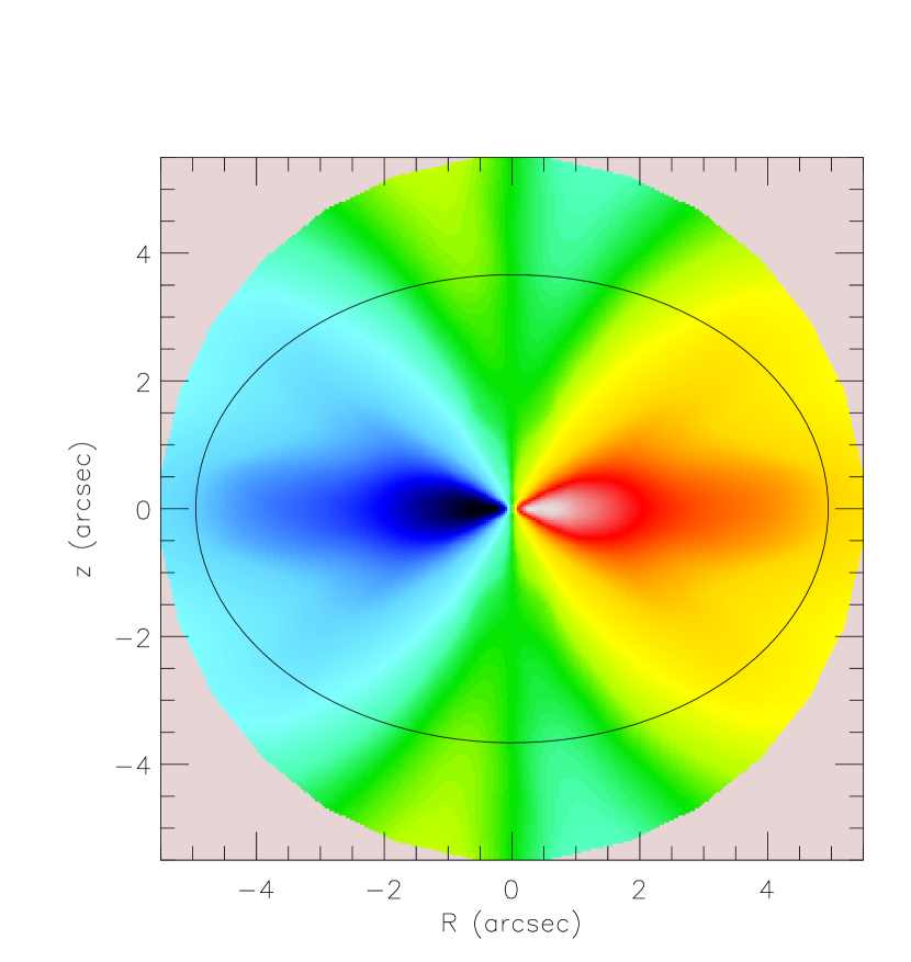
Figure 11: The $V/\sigma$ field in the meridional plane, computed from the velocity moments of the best fitting low regularization ($\Delta=4$) solution of Figure 9. White and black correspond to $V/\sigma=\pm 0.3$, while green indicates the zero velocity curve. The flattened appearance of the $R\lesssim 2$″ counterrotating component is readily apparent. A representative galaxy isodensity contour is also shown. This field was computed from the orbital solution moments on a complete grid in the galaxy meridional plane and was not interpolated from the values in a few aperture positions (as done in Figure 1).

Figure 12: The intrinsic second velocity moments $\left<v_{r}^{2}\right>^{\frac{1}{2}}$ (solid line), $\left<v_{\theta}^{2}\right>^{\frac{1}{2}}$ (dotted line) and $\left<v_{\phi}^{2}\right>^{\frac{1}{2}}$ (dashed line) are plotted as a function of the polar radius in the meridional plane, along sectors linearly spaced in angle between the symmetry axis (upper panel) and the equatorial plane (bottom panel). The moments are normalized by the total RMS velocity $\left<v^{2}\right>^{\frac{1}{2}}$.

Cretton & van den Bosch (1999) showed that the Gauss-Hermite (GH) parametrization for the LOSVD, which is used to constrain the kinematics, can produce artificial counterrotations in some special cases. This is essentially due to the fact that the model is trying to reproduce a small number of GH moments and not the actual observed LOSVD and when two functions coincide on a small set of GH moments this does not guarantee that they are the same function. This phenomenon can be easily recognized after the fit, however, by comparing the LOSVDs predicted by the model and the observed ones. Before interpreting the internal dynamics of IC 1459, we check that our best fit dynamical model does not suffer from this shortcoming.

Figure 13 shows the LOSVD of the model with low regularization ($\Delta=4$), obtained by direct summation on the velocity histograms of the best fitting orbits, together with the observed LOSVD. The latter was reconstructed from the Gauss-Hermite parametrization introduced by van der Marel & Franx (1993), using the mean velocity, the velocity dispersion and the Gauss-Hermite moments that are plotted in Figure 7 and 8. The Hermite polynomials are tabulated in the Appendix C. The plot only represents the most extreme observed LOSVD, but similar results are obtained at the other ground-based apertures. It is apparent from this comparison that the model provides an excellent fit to the observed LOSVD, at least well within the errors suggested by the observed differences in the LOSVD at opposite sides of the galaxy, that are visible in Figure 13. We can thus safely affirm that we are not in the situation of Figure 10 of Cretton & van den Bosch (1999) and that our model reproduces the data correctly.

Figure 13: The LOSVD predicted by the models with low regularization ($\Delta=4$, dashed line) at the radius of maximum observed rotation ($R=\pm 2\farcs 2$), together with the observed LOSVD, which is reconstructed from the first six Gauss-Hermite moments (solid line).

4.2 The STIS gas kinematics

The very central STIS/G430L spectrum of IC 1459 covers the wavelength range between 3500 and 5800 Å. It is dominated by an unresolved source of featureless, non-stellar continuum and by prominent and broad ($\sigma\sim 500$ km s^-1) forbidden gas emission lines of [O II] $\lambda$3727, [Ne III] $\lambda$3869, [S II] $\lambda\lambda$4068,4076, [O III] $\lambda$4363, [O III] $\lambda\lambda$4959,5007, [N I] $\lambda$5200 and the Balmer series emission-lines H$\delta$, H$\gamma$ and H$\beta$. A detailed analysis of the physical properties of this spectrum will be presented elsewhere. In this Section we focus on the gas kinematics.

Of all emission lines, [O II] $\lambda$3727 can be traced reliably to the largest distance from the center ($\sim$1″). Single Gaussians provide a good fit to the emission lines and are therefore used to determine the mean velocity and velocity dispersion at each row of the spectrum (Figure 14, Table 5). The reality of the velocity curve that was determined in this manner can be verified in Figure 15. The line intensity was normalized by dividing each column of the spectrum by the maximum intensity of the [O II] line in that column. The mean velocity curves for the other species agree within the errors with the [O II] line in the regions of overlap. The galaxy nucleus is assumed to be at the peak in the continuum flux. The most salient features are a central steep velocity gradient in the direction opposite to the nuclear stellar rotation and a clear asymmetry of the velocity curve with respect to the nucleus. The velocity curve reaches a peak velocity difference of $\pm 200$ km s^-1, then drops rapidly to zero and even changes sign at $\sim 0\farcs 5$ on one side of the nucleus.

Table 5: IC 1459, PA=34^∘, STIS gas kinematics.

R	$V$	$\Delta V$	$\sigma$	$\Delta\sigma$
(″)	(km s-1)	(km s-1)	(km s-1)	(km s-1)
[O II] $\lambda$3727 emission line
-0.97	20	78	327	79
-0.92	-98	57	243	57
-0.87	1	83	159	83
-0.82	-60	98	202	99
-0.77	-66	126	218	128
-0.72	-117	51	139	51
-0.67	-59	66	307	67
-0.62	15	50	127	50
-0.57	24	35	172	35
-0.52	40	33	179	33
-0.47	74	25	148	25
-0.42	73	19	207	19
-0.37	72	23	284	24
-0.32	142	16	271	16
-0.27	195	12	283	12
-0.22	211	9	295	9
-0.17	215	8	302	9
-0.12	266	11	344	11
-0.07	218	20	423	20
-0.02	18	26	470	26
0.02	-101	15	411	15
0.07	-118	12	326	13
0.12	-122	14	280	14
0.17	-143	12	253	12
0.22	-168	15	277	15
0.27	-213	18	250	18
0.32	-162	22	227	22
0.37	-201	28	299	29
0.42	-208	37	335	38
0.47	-119	33	212	34
0.52	-111	39	211	40
0.57	-185	57	294	58
0.62	-169	60	249	61
0.67	-134	42	214	41
0.72	-135	39	180	40
0.77	-46	51	242	51
0.82	-82	69	324	70
0.87	-3	71	120	71
0.92	-77	55	101	56
0.97	-54	71	293	72
H$\beta$ emission line
-0.32	55	46	100	47
-0.27	166	38	173	39
-0.22	218	30	145	30
-0.17	187	22	193	23
-0.12	278	18	340	19
-0.07	269	45	508	46
-0.02	11	65	532	67
0.02	-66	51	348	53
0.07	-104	47	224	48
0.12	-95	46	211	47
0.17	-165	51	20	52
0.22	-75	97	184	99
0.27	-298	72	181	73

Figure 14: Models of the STIS/G430L gas kinematics. The open circles with error bars represent the observed mean velocity of the gas as measured from the [O II] $\lambda$3727 line, the open squares are the measurements from the H$\beta$ line. Also shown with the filled circles are the measurements by VK00, derived from the H$\alpha$+[N II] blend on the FOS spectra, through the 0$\farcs$086 square apertures. The solid, dotted and dashed lines are the predicted model velocities assuming a disk inclination of $i=60^{\circ}$, $\theta=0^{\circ}$ and a central black hole masses of 0, $3.5\times 10^{8}M_{\odot}$ and $2.6\times 10^{9}M_{\odot}$, respectively. The dash-dotted line is the predicted velocity for a model with $i=20^{\circ}$, $\theta=0^{\circ}$ and $M_{\bullet}=2.6\times 10^{9}M_{\odot}$.

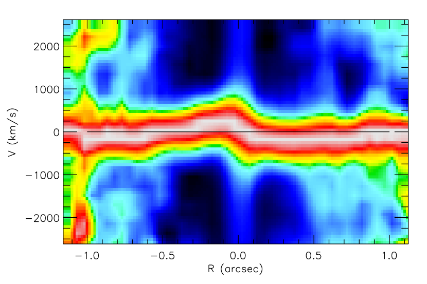
Figure 15: The observed [O II] $\lambda$3727 line on the STIS/G430L spectrum. To make the gas velocity curve more visible, each column of the spectrum was divided by the maximum value of the emission line in that column. The spectrum was then resampled on a $3\times$ finer grid by means of bilinear interpolation.

The asymmetry in the rotation curve with respect to the nucleus prevents a good fit to the complete curve using an axisymmetric gas dynamical model. However, the velocity curve inside $R\lesssim 0\farcs 3$ shows a clear sign of rotation and one might follow standard practice of assuming a gas disk. VK00 obtained 6 FOS emission-line spectra in this region which together with ground-based CTIO emission-line spectra suggested a thin disk in Keplerian rotation. Under this assumption, they determined a BH mass of $M_{\bullet}=1.5\times 10^{8}M_{\odot}$ from a combined best-fit to the H$\beta$ and H$\alpha$+[N II] gas kinematics (scaling their values to our adopted distance). The rotation velocities that VK00 obtained for H$\alpha$+[N II] with the smallest FOS aperture are compared to the STIS results in Figure 14. The data are in broad agreement, but the STIS data clearly provide a more complete and detailed view of the gas kinematics within the central arcsecond. In view of this we have performed a new analysis of the gas kinematics.

We constructed a model for the STIS kinematics using the IDL software we developed in Bertola et al. (1998). The model assumes the gas moves on circular orbits in a thin disk in the galaxy symmetry plane, in the combined potential of the stars and a possible central BH. Our model can deal with a general gas surface brightness distribution (e.g. an observed narrow band image) and takes into account pixel binning, PSF and slit effects to generate a two-dimensional model spectrum with the same pixel scale as the observations. Similar to the observations, the mean model velocity was determined by fitting a Gaussian to each row of the model spectrum. As the STIS observations use the narrow 0$\farcs$1 slit, whose width is comparable to the PSF FWHM, we neglect the velocity offset correction (van der Marel, de Zeeuw, & Rix, 1997; Maciejewski & Binney, 2001; Barth et al., 2001). A detailed comparison between our gas modeling software and the completely independent one used by VK00 shows agreement to better than 5 km s^-1 everywhere, for both $V$ and $\sigma$.

For our STIS model we used the $i=60^{\circ}$ inclination, the parametric approximation of the disk surface brightness and the ‘turbulent’ velocity dispersion parameters as derived by VK00. The stellar potential was determined by deprojecting the axisymmetric MGE fit to the galaxy surface brightness that was used for the stellar kinematic modeling and multiplying this with the best fitting stellar mass-to-light ratio $\Upsilon$. This $\Upsilon$ equals the one used by VK00 (taking into account the differences in assumed distance).

In Figure 14, we compare the gas velocities with models with several different BH masses. The main result is that none of the models properly fits the gas kinematics. This is not entirely surprising, given the somewhat disturbed nature of the gas kinematics, as discussed above. Nonetheless, it is striking to note that the model with $M_{\bullet}=2.6\times 10^{9}M_{\odot}$, the best-fit value inferred from the stellar kinematics, does not even come close to fitting the gas kinematics. It predicts a central rotation curve gradient that is steeper than what is observed and a a rotation curve amplitude that is larger than what is observed. The BH mass must be lowered by a factor of $\sim 7$ to provide a reasonable fit in the central region $R\lesssim 0\farcs 3$. The combined STIS, FOS and CTIO data in this region are best fit by a model with $M_{\bullet}\approx 3.5\times 10^{8}M_{\odot}$. This is somewhat larger than the value inferred by VK00, but is otherwise in reasonable agreement. A model with no BH predicts a rotation curve gradient that is considerably more shallow than what is observed.

4.3 The BH mass discrepancy

Discussions of BH demography have recently focused on the scatter in the relation between BH mass and velocity dispersion. Stellar and gas kinematical BH mass determinations are consistent with the same relation and suggest a scatter of $\sim 0.3$ dex (see e.g. the compilation by Tremaine et al., 2002). It is therefore surprising that our analyses of the stellar and gaseous kinematics in one and the same galaxy have yielded BH masses that differ by a factor $\sim 7$, i.e., $0.9$ dex. To understand the origin of this discrepancy we proceed by discussing the potential systematic problems that may have plagued our analysis.

4.3.1 Possible problems with the interpretation of the gas kinematics

There are several possible reasons why our analysis of the gas kinematics may have yielded an incorrect estimate of the BH mass.

First, it is possible that the underlying assumptions of our model are correct, but that we have used an incorrect value for the inclination of the inner gas disk ($i=60^{\circ}$) or the angle between its projected major axis and the slit ($\theta=0^{\circ}$). These angles are derived from images of the emission-line gas disk at arcsec scales and larger (see VK00 for discussion). However, the ellipticity of the gas disk isophotes in the range 0$\farcs$25–1$\farcs$0 is $\epsilon=$0.17–0.37. VK00 interpreted this as thickening of the gas disk. Alternatively, by allowing the disk to be actually more face-on, the ellipticity is consistent with inclinations between $\sim 10^{\circ}$ and $22^{\circ}$. By constructing models for various $(i,\theta)$, we find that a model with $i\sim 20^{\circ}$, $\theta\sim 0^{\circ}$ and $M_{\bullet}=2.6\times 10^{9}M_{\odot}$ indeed provides a reasonable and much better fit to the STIS mean gas velocities at $R\lesssim 0.3^{\prime\prime}$ than a model with $M_{\bullet}=3.5\times 10^{8}M_{\odot}$ (Figure 14). However, this interpretation implies that the gas disk is warped (e.g. Statler 2001) and that it cannot reside in the equatorial plane of the galaxy for $R\lesssim 1^{\prime\prime}$ (the galaxy inclination cannot be lower than $i\lesssim 55^{\circ}$: see Section 4.1). Although the spherical BH potential dominates the galaxy potential for $R\lesssim 0\farcs 65$, the severe warping likely invalidates the assumption of a thin circular gas disk in equilibrium.

Second, it is possible that the underlying assumptions of our model are incorrect, and that the gas does not move on circular orbits in an infinitely thin disk. In our models we have assumed that the observed velocity dispersion of the gas is ‘turbulent’ and does not contribute to its hydrostatic support. However, it may be that the gas is better modeled as individual clouds that move ballistically. In this case the velocity dispersion would contribute to the hydrostatic support and the gas would rotate slower than the circular velocity (asymmetric drift). This would have caused our models to underpredict the BH mass. If $\sigma/V$ is small, then the upward correction to the BH mass is small and it can be estimated using approximate equations for asymmetric drift (e.g. Barth et al., 2001). However, for IC 1459 the value of $\sigma/V$ of order unity, and to properly estimate the BH mass one would have to construct axisymmetric collisionless models for the gas kinematics. This is outside the scope of the present paper. However, one limiting case that can be calculated fairly easily is to assume that the gas can be modeled through the Jeans equations as an isotropic spherical distribution of collisionless cloudlets. This may not be entirely unreasonable, given that the isophotes of the gas disk become rounder towards the center. We find that the BH mass must then be $M_{\bullet}\approx 1.0\times 10^{9}M_{\odot}$ to reproduce the observed central velocity dispersion of the gas (this supersedes the somewhat smaller value that we quoted for this scenario in VK00).

Third, it is possible that our models for the gas kinematics of IC 1459 are flawed at an even more basic level. The gas may not be in equilibrium. The fact that IC 1459 has a counter-rotating core, possibly indicative of a recent accretion event, may be of relevance in this context. Or alternatively, the gas kinematics (mean velocities and velocity dispersions) may not be dominated by gravitational forces. For galaxies in which the central emission-line gas displays a LINER-type spectrum the gas excitation mechanism might be shock-ionization (e.g. Dopita et al., 1997) as opposed to photo-ionization (as inferred for Seyferts and Quasars). IC 1459 indeed shows LINER-type emission and hence shocks may influence the gas kinematics.

IC 1459 was originally identified by us as a good candidate for thin-disk modeling because of the regular, smooth and prominent rotation evident in ground-based CTIO spectra. With FOS, spectra could only be obtained for a few individual apertures (VK00). This yielded insufficient information to test the hypothesis that the gas is indeed rotating in a thin disk. The new STIS spectra provide a more complete view of the gas disk kinematics and clearly show that thin disk models are oversimplified. The gas does not rotate at all at $R\approx 1^{\prime\prime}$, indicating that the true state of the gas must be considerably more complicated than what we have been able to represent in any of our models. In hindsight, IC 1459 is a poor galaxy for which to attempt a gas kinematical determination of the central BH mass. The values that we have inferred range from $\sim 3.5\times 10^{8}M_{\odot}$ (thin gas disk) to $\sim 1.0\times 10^{9}M_{\odot}$ (spherical distribution of cloudlets), but we cannot attach strong confidence to either of these numbers.

4.3.2 Possible problems with the interpretation of the stellar kinematics

The highest spatial resolution stellar kinematical data presented here are based on a STIS spectrum obtained in 4 orbits of HST time. While this is a significant exposure time, the S/N of the spectrum is relatively low (due mostly to the very narrow slit employed). This has several consequences. The low S/N, the relatively low spectral resolution, and the presence of prominent gas emission lines filling important absorption features, prevent the reliable extraction of higher-order Gauss–Hermite moments. As a result, we can only obtain the mean velocity $V$ and velocity dispersion $\sigma$ of the best-fit Gaussian, with error bars that are considerably larger than those for the ground-based kinematics. Furthermore, the unresolved source of featureless non-thermal continuum that dominates the central spectrum of IC 1459 prevents the measurement of the stellar kinematics inside 0$\farcs$1. The latter is particularly unfortunate, because the influence of a BH is always expected to be largest close to the galaxy center.

The $V$ and $\sigma$ profiles derived from the STIS spectrum (for $R\gtrsim$0$\farcs$1) do not show any obvious evidence for the presence of a BH (Figure 8). While the central velocity gradient is steeper than the one measured from the ground, there is no strong central increase in $\sigma$. Also, the value of $\sigma$ at 0$\farcs$1 is no larger than the central dispersion observed from the ground. This might suggest a low black hole mass, and indeed, a dynamical model with the value, derived from the gas kinematics, of $M_{\bullet}=3.5\times 10^{8}M_{\odot}$, is consistent with the STIS data. However, our model with the much larger mass of $M_{\bullet}=2.6\times 10^{9}M_{\odot}$ (inferred from our analysis of all the stellar kinematical data) is also consistent. The reason for this surprising fact can be understood by considering the LOSVD predicted by the model with $M_{\bullet}=2.6\times 10^{9}M_{\odot}$ for the STIS apertures closest to the center ($R=\pm 0\farcs 10$; Fig. 16). It is strongly non-Gaussian and has very broad wings, caused by the high-velocity stars near the central BH. Qualitatively similar profiles, close to the BH, were predicted with analytic models (e.g. van der Marel, 1994a) and have been observed with HST since (e.g. Joseph et al., 2001). Figure 17 shows that the true centered moment $\sigma_{\rm true}$ displays a large increase inside the BH sphere of influence ($R_{\rm BH}\approx 0\farcs 65$). This rise is absent in $\sigma$ because the best-fitting Gaussian is quite insensitive to the wings, and as a result the model can fit the flat $\sigma$ profile even with a large black hole mass.

Figure 16: The LOSVD predicted by the Schwarzschild modeling with low regularization ($\Delta=4$, dashed line) at the smallest measured radii ($R=\pm 0\farcs 10$) within the STIS slit along the major axis, is compared to the Gaussian measured from the STIS spectrum (solid line). In both panels the true centered second order moment is $\sigma_{\rm true}\approx 422$ km s^-1, while the dispersion of the best fitting Gaussian is $\sigma\approx 325$ km s^-1.

Figure 17: Top Panel: The true centered second moment $\sigma_{\rm true}$ predicted by the Schwarzschild modeling, within the STIS slit along the major axis, for the model with $M_{\bullet}=3.5\times 10^{8}M_{\odot}$ (dashed line with triangles) and with $M_{\bullet}=2.6\times 10^{9}M_{\odot}$ (solid line with open squares). The predictions for the central aperture ($R=0$), where we have no data, is also shown. Bottom Panel: Same as in top panel for the dispersion $\sigma$ of the best fitting Gaussian.

As a further check of the consistency of our $M_{\bullet}=2.6\times 10^{9}M_{\odot}$ dynamical model with the STIS observations, we convolved a well-sampled K3 III stellar template with the predicted model LOSVD at the different apertures along the STIS slit and rebinned this to the STIS pixel scale. The spectrum thus obtained was processed through the same procedure, described in Section 2.1, to extract the $V$ and $\sigma$. The resulting values agree to within the errors with the model profiles presented in Figure 8.

For the above reasons, our black hole mass estimate is determined primarily by the ground-based data. Our axisymmetric models take into account the limited spatial resolution of the data, and they formally rule out the BH mass $M_{\bullet}=3.5\times 10^{8}M_{\odot}$ that was suggested by the gas kinematics. This comes about because the central $\sigma$ measured from the ground is larger than the models can handle with a black hole mass of less than $\sim 10^{9}M_{\odot}$, while also fitting the higher order moments. However, Fig. 18 shows just how small this effect is. The effect is formally quite significant, but this assumes that there are no uncertainties involved in the data-model comparison other than Gaussian random errors. This is obviously an oversimplification. On the one hand, the underlying assumptions of the models may not be fully correct. For example, IC 1459 could be significantly triaxial, the stars may not yet have settled into an equilibrium configuration, or line-of-sight projections may be partially compromised by dust. On the other hand, there could be systemic problems with the data, e.g., due to continuum subtraction or template mismatching. Such effects can easily compromise the data at the few percent level (van der Marel et al., 1994c). Since the very central region is affected by a continuum component that is not present at larger radii, it is quite possible that these errors could depend on radius. While there are no obvious indications that any of these issues may be affecting our analysis, it does mean that our BH mass determination via the stellar kinematics should be treated with caution.

Figure 18: Comparison of the velocity dispersion profiles for the dynamical models with $M_{\bullet}=3.5\times 10^{8}M_{\odot}$ (dotted line) and with $M_{\bullet}=2.6\times 10^{9}M_{\odot}$ (solid line). This profile corresponds to the central part of the intermediate axis ground-based measurements and is also shown in the last column of Fig. 7. The central $\sigma$ predicted by the model with lower BH mass is always at least one standard deviation below the measured value, for all observations along five position angles. Assuming Gaussian errors and considering only the central $\sigma$ measurements, the model with lower BH mass would be excluded at better than the $3\sigma$ level.

The accuracy of stellar dynamical BH mass determinations hinges critically on the availability of full LOSVD measurements inside the BH sphere of influence. Unfortunately, we have not been able to secure such a measurements with HST due to the complications introduced by the modest $S/N$, the presence of a non-thermal nuclear point source and of strong gas emission lines. Our BH mass measurement $M_{\bullet}=(2.6\pm 1.1)\times 10^{9}M_{\odot}$ therefore rests primarily on $\sim 1.5^{\prime\prime}$ resolution ground-based spectroscopy. This makes the accuracy of our measurement rather modest, despite the use of three-integral models and the well-defined formal errorbar.

5 Discussion and conclusions

We studied the dynamics of the elliptical galaxy IC 1459 using self-consistent axisymmetric dynamical models based on Schwarzschild’s orbit superposition method. The intrinsic density is obtained by deprojecting the observed HST/WFPC2 surface density using an MGE parametrization, after correction for the effects of patchy dust absorption. The axisymmetric model provides an excellent fit to all HST and ground-based kinematical constraints along five slit positions, while also matching the observed HST photometry. Moreover we verified that the model velocity histograms indeed reproduce the observed LOSVDs and not only its moments.

The good match to the observations obtained with an axisymmetric model provides a test that the counterrotating core in IC 1459 can be accurately described as an axisymmetric stellar component. We explored the $\chi^{2}$ map as a function of the three free parameters of the problem $(i,\Upsilon,M_{\bullet})$ and subsequently analyzed the best fit solution by adding linear regularization constraints in the integral space. The observations can only be reproduced if $\approx 0.5$% of the galaxy stellar mass ($\approx 3\times 10^{9}M_{\odot}$) counterrotates in the radial range $R\,\lesssim\,2\arcsec$ on nearly circular orbits in a flattened disk. This counterrotating component is found to be very well separated from the bulk of the stars in integral space. The mass estimation of the counterrotating stellar component is only possible by using dynamical modeling, since the decoupled component does not show in the surface brightness or color maps and cannot be isolated from the observed line profiles.

These results could be explained by a scenario in which the stellar counterrotating core in IC 1459 has an external origin, as evidenced by its clear isolation in integral space from the bulk of the stars in the galaxy. For example, the core may have formed by acquisition of a gas-rich component that settled into a disk in the galaxy potential and later turned into stars. In this scenario it is likely that the acquisition must have happened long ago. The current stellar core counterrotates not only with respect to the outer stellar body but also with respect to the nuclear gas-disk of IC 1459, which must have formed later. Numerical simulations of gas accretion by a BH that leads to disk formation and BH fueling were made by e.g. Bekki (2000) However, other formation scenarios are also possible. For example, Holley-Bockelmann & Richstone (2000) showed that, in the presence of a central BH, a rapidly rotating counterrotating core can also be produced by acquisition of a dense stellar satellite.

IC 1459 has a rotating gas component near its center. This offers the opportunity to estimate the BH mass independently from either gaseous or stellar kinematics. For both we have available high spatial resolution long-slit kinematics from STIS, as well as ground-based kinematics along multiple position angles. Unfortunately, we have found that neither the gaseous nor the stellar kinematics yield a very stringent determination of the BH mass. The main problem for the gas kinematical modeling is that there is evidence that the gas motions are disturbed, possibly due to non-gravitational forces acting on the gas. The main problem for the stellar kinematical modeling is that we were unable to obtain an HST measurement of the stellar LOSVD inside the BH sphere of influence, due to the modest $S/N$ of our STIS spectrum and due to the presence of the non-thermal nuclear point source of IC 1459 and prominent gas emission lines. Consequently, the stellar dynamically inferred BH mass hinges almost exclusively on the low spatial-resolution ground-based data. These complications may explain why we find rather discrepant BH masses with the different methods. The gas kinematics suggests that $M_{\bullet}=3.5\times 10^{8}M_{\odot}$ if the gas is assumed to rotate at the circular velocity in a thin disk. Alternatively, the central velocity dispersion of the gas implies that $M_{\bullet}=1.0\times 10^{9}M_{\odot}$ if the gas is modeled as an isotropic spherical distribution of ballistic cloudlets. The stellar kinematics suggest that $M_{\bullet}=(2.6\pm 1.1)\times 10^{9}M_{\odot}$. These different estimates bracket the value $M_{\bullet}=(1.1\pm 0.3)\times 10^{9}M_{\odot}$ predicted by the $M_{\bullet}$-$\sigma$ relation (Ferrarese & Merritt, 2000; Gebhardt et al., 2000) as given by Tremaine et al. (2002).

To our knowledge, IC 1459 is only the second galaxy (Pinkney et al. 2000 modeled NGC 4697) for which a BH mass determination has been attempted with HST observations of both gaseous and stellar kinematics. Unfortunately, as it turned out, IC 1459 may not been the best galaxy to attempt such a comparison. However, it certainly is important to perform such comparisons. They provide insight into the reliability of BH mass determinations, which is necessary to properly understand the correlation between the BH mass correlation and other global galaxy parameters (Tremaine et al. 2002 and the refs therein). This is particularly relevant if one wants to understand the scatter in such relations and their implications for our understanding of the galaxy formation process.

With the availability of 2D spectroscopic detectors (e.g. SAURON on WHT, VIMOS on VLT, GMOS on Gemini) it is possible to obtain fully two-dimensional distributions of LOSVDs and line-strengths of kinematically decoupled cores (e.g. Davies et al., 2001; de Zeeuw et al., 2002). These observations will provide a much larger number of kinematical constraints than can be obtained from a small number of slit positions, which results in dynamical models that better constrain the model parameters (e.g. Verolme et al., 2002), especially if they resolve the radius of influence of the BH. In turn, this will improve the reliability of internal dynamical studies such as that presented in this paper.

Appendix A MGE potential calculation

In this Appendix, we discuss the techniques that were used to efficiently and accurately evaluate the MGE potential. The MGE surface brightness defined in equation (2) can be deprojected analytically (Monnet et al., 1992) to derive an axisymmetric intrinsic luminosity density consistent with the observations. Using the equations in Cappellari (2002) the intrinsic luminosity density can be written as

$$\rho(R,z)=\sum_{j=1}^{N}\frac{L_{j}}{(\sigma_{j}\,\sqrt{2\pi})^{3}q_{j}}\exp\left[-\frac{1}{2\sigma_{j}^{2}}\left(R^{2}+\frac{z^{2}}{q_{j}^{2}}\right)\right],$$ (A1)

where $N$ is the number of Gaussians required in the expansion, $L_{j}$ is the Gaussian total luminosity, $\sigma_{j}$ the corresponding dispersion and the intrinsic axial ratio $q_{j}=\sqrt{q^{\prime 2}_{j}-\cos^{2}i}/\sin i$, where $i$ is the galaxy inclination.

The general form for the potential that corresponds to an MGE density profile is

$$\Psi(R,z)=G\Upsilon\sqrt{2/\pi}\;\sum_{j=1}^{N}{\frac{L_{j}\,{\mathcal{Q}}_{j}(R,z)}{\sigma_{j}}}$$ (A2)

(Emsellem et al., 1994), with

$${\mathcal{Q}}_{j}(R,z)=\int_{0}^{1}{\frac{{\exp\left\{-\frac{{T^{2}}}{{2\sigma_{j}^{2}}}\left[{R^{2}+\frac{{z^{2}}}{{1-(1-q_{j}^{2})T^{2}}}}\right]\right\}}}{{\sqrt{1-(1-q_{j}^{2})T^{2}}}}\mathrm{d}T}.$$ (A3)

Since the Gaussians of an MGE parametrization sample many orders of magnitude in radius, it is worthwhile to check if it is necessary to do the actual integration in equation (A3) or whether a limiting expression can be used instead. We desire a maximum relative error of $\epsilon\,\lesssim\,10^{-4}$ for the potential. This is at least two orders of magnitude more accurate than what can generally be achieved for photometric measurements.

An approximate expression for the potential at large radii can be found using a multipole expansion of the potential (e.g. Binney & Tremaine, 1987). Terminating the expansion at the first term, ${\mathcal{Q}}_{j}(R,z)$ in equation (A3) equals

$${\mathcal{Q}}_{j}(R,z)=\frac{\sigma_{j}\,\sqrt{\frac{\pi}{2}}}{\sqrt{R^{2}+z^{2}}},$$ (A4)

and the potential reduces to the potential of a point mass with mass $\mathcal{M}=\Upsilon L_{j}$. Even in the thin disk limit, a maximum relative error $\epsilon\,\lesssim\,10^{-4}$ is obtained outside the sphere $100\,\sigma_{j}\lesssim\sqrt{R^{2}+z^{2}}$. In the case of positive Gaussians this is a conservative estimate for the total relative error in the potential, since it applies only to one Gaussian, while in practice not all Gaussians in the expansion will be in the least favorable condition at the same time. This error limitation is generally not true when the MGE is composed by both positive and negative Gaussians, due to cancellation effects.

An approximate expression for the potential at small radii can be obtained by calculating a Taylor expansion of the $\exp(x)$ term in equation (A3) around $x=0$. The first term in this expansion equals

$${\mathcal{Q}}_{j}(R,z)=\frac{\arcsin\left({\sqrt{1-q_{j}^{2}}}\right)}{{\sqrt{1-q_{j}^{2}}}}.$$ (A5)

This corresponds to replacing the potential by its central analytic value $\Psi(0,0)$. Assuming a lower limit on the axial ratio $0.1<q_{j}$ a maximum relative error $\epsilon\,\lesssim\,10^{-4}$ is obtained inside the sphere $\sqrt{R^{2}+z^{2}}\lesssim\,\sigma_{j}/171$.

An example of the usefulness of this approximation is given by the present application. Our orbit grid spans the radial range $0\farcs 05<R<300\arcsec$; a comparison with Table 4 therefore shows that these approximations are used often and only a small number of integrations has to be carried out. A related advantage of this is that the regions where the approximations are used are precisely those where the integrand is badly behaved and the numerical integration may become inaccurate.

Similar considerations are valid for the two components of the acceleration in the meridional plane, which are required by the orbit integration.

When the integral in equation (A3) has to be evaluated, we use a globally adaptive, recursive Gauss-Kronrod integration scheme (Favati, Lotti, & Romani, 1991). The use of such an algorithm is very beneficial at small and large distances from the galaxy center (but before the switch to the limiting regimes), where the integrand of equation  (A3) shows a sharp peak close to $T=1$ or to $T=0$ respectively. In these cases the integrand is evaluated more densely around the peaks.

Appendix B Integration of a Gaussian on a grid

Axisymmetric Schwarzschild modeling is aimed at finding the linear combination of orbits that reproduces the observed kinematics at various apertures, the intrinsic density $\rho(R,z)$ on the meridional plane and, to limit the effect of discretization, also the surface density $\Sigma(x,y)$ on the projected plane. In general, the comparison with the density requires a double or triple integration. However, these computations can be simplified for an MGE parametrization. We discuss the different cases below. We always assume that the Gaussians have a maximum value of one, which means that intrinsic quantities have to be multiplied by $L_{j}/[(\sigma_{j}\,\sqrt{2\pi})^{3}q_{j}]$ and projected quantities by $L_{j}/(2\pi\,\sigma_{j}^{2}q^{\prime}_{j})$ (see Cappellari, 2002, for details). In the following equations, the index has been dropped from the $\sigma_{j}$ and $q_{j}$ variables and $q$ has to be substituted by $q^{\prime}$ when dealing with projected plane quantities.

B.1 Polar grid in the meridional plane

We integrate an axisymmetric three dimensional Gaussian defined by $\rho(R,z)$ in equation (A1) on the “torus” $D$ of Figure 19 around the galaxy symmetry axis, which is delimited by the intervals $[r_{0},r_{1}]$ and $[\theta_{0},\theta_{1}]$ in spherical coordinates ($\theta=0$ on the symmetry axis). The integrated mass is given in spherical coordinates by

$$\int_{D}\rho\,=\,2\pi\int_{\theta_{0}}^{\theta_{1}}\int_{r_{0}}^{r_{1}}e^{-(r/c(\theta))^{2}}\,r^{2}\,\sin\theta\mathrm{d}r\,\mathrm{d}\theta$$ (B1)

where $c(\theta)=2\,q\,\sigma\,/\sqrt{1+q^{2}+(1-q^{2})\cos 2\theta}$. The innermost integral can be performed analytically and the integral becomes

$$\pi\,\int_{\theta_{0}}^{\theta_{1}}\bigg{\{}\frac{c(\theta)\sqrt{\pi}}{2}\,\left[{\rm erf}\left(\frac{r_{1}}{c(\theta)}\right)-{\rm erf}\left(\frac{r_{0}}{c(\theta)}\right)\right]+r_{0}\,e^{-(r_{0}/c(\theta))^{2}}-\,r_{1}\,e^{-(r_{1}/c(\theta))^{2}}\bigg{\}}\,c(\theta)^{2}\,\sin\theta\mathrm{d}\theta$$ (B2)

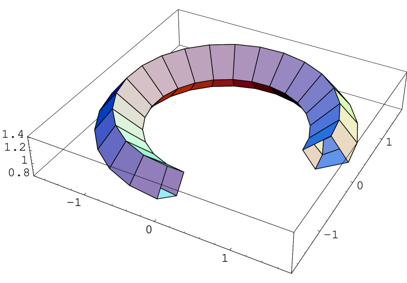
Figure 19: One of the elements of the meridional plane grid. Equation  B2 represents the mass of an axisymmetric Gaussian contained within this region. One quadrant has been removed from the element for display purposes.

B.2 Polar grid in the projected plane

In the case of the integration of a two dimensional Gaussian on a polar cell $D$, delimited by the intervals $[r_{0},r_{1}]$ and $[\theta_{0},\theta_{1}]$ in polar coordinates, we have to compute the integral

$$\int_{D}\Sigma\,=\,\int_{\theta_{0}}^{\theta_{1}}\int_{r_{0}}^{r_{1}}e^{-(r/c(\theta))^{2}}\,r\,\mathrm{d}r\,\mathrm{d}\theta,$$ (B3)

where $\theta=0$ on the Gaussian minor axis, which gives

$$\int_{\theta_{0}}^{\theta_{1}}\frac{c(\theta)^{2}}{2}\left[e^{-(r_{0}/c(\theta))^{2}}-e^{-(r_{1}/c(\theta))^{2}}\right]\mathrm{d}\theta.$$ (B4)

B.3 Cartesian grid on the projected plane

We compute the integral of a two-dimensional Gaussian on a Cartesian grid cell $D$ delimited by the intervals $[x_{0},x_{1}]$ and $[y_{0},y_{1}]$. Assuming the cell is parallel to the Gaussian major axis, the integral is given by

$$\int_{D}\Sigma\,=\,\frac{\pi\,q\,\sigma^{2}}{2}\left[{\rm erf}\left(\frac{x_{0}}{\sigma\sqrt{2}}\right)-{\rm erf}\left(\frac{x_{1}}{\sigma\sqrt{2}}\right)\right]\left[{\rm erf}\left(\frac{y_{0}}{q\,\sigma\sqrt{2}}\right)-{\rm erf}\left(\frac{y_{1}}{q\,\sigma\sqrt{2}}\right)\right].$$ (B5)

If the Gaussian major axis makes an angle $\theta$ with the $x$ axis, the double integral on the grid cannot be evaluated explicitly, but can still be expressed as a single integral in one of the coordinates as follows

$$\frac{q\,\sigma\sqrt{\pi}}{p}\!\int_{x_{0}}^{x_{1}}\!\!\left[{\rm erf}\!\left(\frac{f_{0}(x)}{2pq\sigma}\right)\!\!-\!{\rm erf}\!\left(\frac{f_{1}(x)}{2pq\sigma}\right)\right]\!e^{-[x/(p\,\sigma)]^{2}}\mathrm{d}x,$$ (B6)

with $p=\sqrt{1+q^{2}+(1-q^{2})\cos 2\theta}$, and we defined

$$f_{k}(x)=(1-q^{2})\,x\,\sin 2\theta-p^{2}\,y_{k}\qquad{\rm for}\qquad k=0,1.$$ (B7)

Appendix C Hermite polynomials

We tabulate the first seven Hermite orthogonal polynomials, following the normalization of van der Marel & Franx (1993). They are written in Horner form for efficient and stable evaluation. The first five are also given in equation (A5) of that paper.

$$H_{0}(y) = 1,\quad H_{1}(y)={\sqrt{2}}\,y,\quad H_{2}(y)=\frac{2\,y^{2}-1}{{\sqrt{2}}},\quad H_{3}(y)=\frac{y\,\left(2\,y^{2}-3\right)}{{\sqrt{3}}},$$

$$H_{4}(y) = \frac{y^{2}\,\left(4\,y^{2}-12\right)+3}{2\,{\sqrt{6}}},\quad H_{5}(y)=\frac{y\,\left[y^{2}\,\left(4\,y^{2}-20\right)+15\right]}{2\,{\sqrt{15}}},$$

$$H_{6}(y) = \frac{y^{2}\,\left[y^{2}\,\left(8\,y^{2}-60\right)+90\right]-15}{12\,{\sqrt{5}}}.$$ (C1)

References

- Barth et al. (2001) Barth, A. J., Sarzi, M., Rix, H.-W., Ho, L. C., Filippenko, A. V., & Sargent, W. L. W. 2001, ApJ, 555, 685
- Bekki (2000) Bekki, K. 2000, ApJ, 545, 753
- Bertola et al. (1998) Bertola, F., Cappellari, M., Funes, J. G., Corsini, E. M., Pizzella, A., & Vega Beltrán, J. C. 1998, ApJ, 509, L93
- Binney & Tremaine (1987) Binney, J. J., & Tremaine, S. D. 1987, Galactic Dynamics (Princeton, NJ: Princeton Univ. Press)
- Burkert (1993) Burkert, A. 1993, A&A, 278, 23
- Cappellari (2000) Cappellari, M. 2000, PhD thesis, Padova University
- Cappellari (2002) Cappellari, M. 2002, MNRAS, 333, 400
- Cappellari et al. (2001) Cappellari, M., Verolme, E. K., van der Marel, R. P., Verdoes Kleijn, G. A., Franx, M., Carollo, C. M., & de Zeeuw, P. T. 2001, in ASP Conf. Ser. 230, Galaxy Disks and Disk Galaxies, ed. J. G. Funes & E. M. Corsini (San Francisco: ASP), 439
- Cardelli et al. (1989) Cardelli, J. A., Clayton, G. C., & Mathis, J. S. 1989, ApJ, 345, 245
- Carollo et al. (1995) Carollo, C. M., de Zeeuw, P. T., van der Marel, R. P., Danziger, I. J., & Qian, E. E. 1995, ApJ, 441, L25
- Carollo et al. (1997) Carollo, C. M., Franx, M., Illingworth, G. D., & Forbes, D. A. 1997, ApJ, 481, 710, (C97)
- Charlot et al. (1996) Charlot, S., Worthey, G., Bressan, A. 1996, ApJ, 457, 625