Photon-axion oscillations and Type Ia supernovae

I Abstract

We compute the probability of photon-axion oscillations in the presence of both intergalactic magnetic fields and an electron plasma and investigate the effect on Type Ia supernovae observations. The conversion probability is calculated using a density matrix formalism by following light-paths through simulated universes in a Monte-Carlo fashion. We find, that even though the effect is highly frequency dependent, one needs to analyze relatively narrow spectral features of high redshift objects in order to discern between the dimming effect from oscillations and a cosmological constant, in contrast to earlier claims that broad-band photometry is sufficient.

PACS numbers: 13.40.Hq, 98.80.Es, 97.60.Bw

II Introduction

Recently, Csáki, Kaloper and Terning [1] (CKT) proposed that the observed faintness of high redshift supernovae (SNe) could be attributed to the mixing of photons with a light axion in an intergalactic magnetic field. The nature of the oscillations is governed by the strength of the coupling which in turn depends on the axion coupling constant mass scale, the photon energy and the strength of the magnetic field. Assuming magnetic domains with uncorrelated field direction of size $\sim$ Mpc, CKT found that for optical photons the oscillation is maximal and independent of energy, i.e., in the limit of infinite travel distance one approaches an equilibrium between the two photon polarization states and the axion. For optical photons, the probability to detect a photon as a function of the traveled distance, $l$, was approximated as

$$P_{\rm\gamma}\simeq\frac{2}{3}+\frac{1}{3}\exp{(-l/l_{\rm 0})},$$ (1)

where $l_{\rm 0}$ is the exponential decay-length. It was claimed that since this effect will cause additional dimming of high redshift SNe, constraints on the equation of state parameter of the dark energy component could be significantly relaxed. (The presence of a non-clustering component of “dark energy” has recently been independently inferred from a combination of measurements of the cosmic microwave background and the distribution of galaxies on large scales. The proposed photon-axion mixing does not remove the need for such a component, but its equation of state need not be as close to that for a cosmological constant as is the case without such a mixing.) For low photon energies, the oscillation was found to be energy dependent and the mixing very small. Therefore it should not severely affect the cosmic microwave background radiation which is redshifted to low energies at low $z$ where the magnetic fields appear. For a magnetic field strength of $|\vec{B}|\sim 10^{-9}$ G, CKT found that the current data can be accommodated by $\Omega_{\rm M}=0.3,\Omega_{\rm X}=0.7,\omega_{\rm X}=-1/3$ if the axion mass is $m\sim 10^{-16}$ eV and the coupling scale is $M\sim 4\cdot 10^{11}$ GeV.

It was then pointed out by Deffayet, Harari, Uzan and Zaldarriaga [2] that one has to take the effect of the intergalactic plasma into account, i.e., the free electrons, in which the photons are propagating. For a mean electron density of $n_{\rm e}\sim 10^{-7}\,{\rm cm}^{-3}$, they found that this will alter (lower) the oscillation probability and may also cause the oscillations for optical photons to be frequency dependent to a degree where the effect can be ruled out by observational constraints, namely by studying the color excess between the $B$ and $V$ wavelength bands. Only for very definitive properties of the intergalactic magnetic field could one get a large enough mixing angle and weak enough frequency dependence, namely with $|\vec{B}|\sim 10^{-8}$ G over domains of size $\sim 10$ kpc and weaker magnetic field strength over larger domains. (The strength and spatial properties of intergalactic magnetic are not well constrained by present measurements, for a recent review see [3].)

In a reply, Csáki et al. [4] pointed out that the mean electron density in most of space realistically is lower than the estimate used by Deffayet et al. by a factor of at least 15. Since the energy dependence of the oscillations is very sensitive to this value, they find that this factor is enough to bring the energy dependence within current experimental bounds.

In this note, we perform a full density matrix calculation of the photon-axion oscillations and find the conversion probability to be highly frequency dependent and also not necessarily monotonically increasing with increasing redshift. We also calculate the color excess between different wavelength bands for Type Ia SNe by integrating over spectrum templates modified by performing the density matrix calculation over the appropriate frequency range (taking the redshifting of the spectra into account).

III Density matrix formalism

We compute the mixing probability using the formalism of density matrices (see, e.g., [7]). Following the notation of [2], we define the mixing matrix as

$$M=\left(\begin{array}[]{ccc}\Delta_{\perp}&0&\Delta_{\rm M}\cos\alpha\\ 0&\Delta_{\parallel}&\Delta_{\rm M}\sin\alpha\\ \Delta_{\rm M}\cos\alpha&\Delta_{\rm M}\sin\alpha&\Delta_{\rm m}\end{array}\right).$$ (2)

The different quantities appearing in this matrix are given by

$$\Delta_{\perp} = -3.6\times 10^{-25}\left(\frac{\omega}{1\,{\rm eV}}\right)^{-1}\left(\frac{n_{\rm e}}{10^{-8}\,{\rm cm}^{-3}}\right){\rm cm}^{-1},$$ (3)

$$\Delta_{\parallel} = \Delta_{\perp},$$ (4)

$$\Delta_{\rm M} = 2\times 10^{-26}\left(\frac{B_{\rm 0,\perp}}{10^{-9}\,{\rm G}}\right)\left(\frac{M_{\rm a}}{10^{11}\,{\rm GeV}}\right)^{-1}{\rm cm}^{-1},$$ (5)

$$\Delta_{\rm m} = -2.5\times 10^{-28}\left(\frac{m_{\rm a}}{10^{-16}\,{\rm eV}}\right)^{2}\left(\frac{\omega}{1\,{\rm eV}}\right)^{-1}{\rm cm}^{-1},$$ (6)

where $B_{\rm 0,\perp}$ is the strength of the magnetic field perpendicular to the direction of the photon, $M_{\rm a}$ is the inverse coupling between the photon and the axion, $n_{\rm e}$ is the electron density, $m_{\rm a}$ is the axion mass and $\omega$ is the energy of the photon. The angle $\alpha$ is the angle between the (projected) magnetic field and the (arbitrary, but fixed) perpendicular polarization vector. Our standard set of parameter-values is given by

$$B_{\rm 0} = 10^{-9}(1+z)^{2}\,{\rm G},$$ (7)

$$M_{\rm a} = 10^{11}\,{\rm GeV},$$ (8)

$$m_{\rm a} = 10^{-16}\,{\rm eV},$$ (9)

$$n_{\rm e}(z) = 10^{-8}(1+z)^{3}\,{\rm cm}^{-3},$$ (10)

with a 20 % dispersion in $B_{0}$ and $n_{\rm e}$ and the redshift dependence of the magnetic field strength and the electron density comes from flux conservation and cosmological expansion, respectively. The equation to solve for the evolution of the density matrix $\rho$ is given by

$${\rm i}\delta_{\rm t}\rho=\frac{1}{2\omega}[M,\rho],$$ (11)

with initial conditions

$$\rho_{\rm 0}=\left(\begin{array}[]{ccc}\frac{1}{2}&0&0\\ 0&\frac{1}{2}&0\\ 0&0&0\end{array}\right).$$ (12)

Here the three diagonal elements refer to two different polarization intensities and the axion intensity, respectively. We solve the system of 9 coupled (complex) differential equations numerically [8], by following individual light paths through a large number of cells where the strength of the magnetic field and the electron density is determined from predefined distributions and the direction of the magnetic field is random. Through each cell the background cosmology and the wavelength of the photon are updated, as well as the matrices $\rho$ and $M$.

In order to study the qualitative behavior of the solutions, we rewrite $M$ as a $2\times 2$ matrix,

$$M^{\rm 2D}=\left(\begin{array}[]{ccc}\Delta&\Delta_{\rm M}\\ \Delta_{\rm M}&\Delta_{\rm m}\end{array}\right),$$ (13)

where $\Delta=\Delta_{\perp}=\Delta_{\parallel}$ and $\Delta_{\rm M}$ is the component of the magnetic field parallel to the some average polarization vector of the photon beam. We solve Eq. 11 for the density matrix $\rho^{\rm 2D}$ with initial conditions

$$\rho_{\rm 0}=\left(\begin{array}[]{cc}1&0\\ 0&0\end{array}\right),$$ (14)

where the diagonal elements refer to the photon and the axion intensity respectively. Assuming a homogeneous magnetic field and electron density, we can solve the two-dimensional system analytically. For the $\rho^{\rm 2D}_{11}$ component, referring to the photon intensity, we get

$$\rho^{\rm 2D}_{11} = 1-\left(\frac{\Delta_{\rm M}}{2\omega\Omega}\right)^{2}(1-\cos{\Omega t}),$$ (15)

$$\Omega = \frac{\sqrt{(\Delta-\Delta_{\rm m})^{2}+2\Delta_{\rm M}^{2}}}{2\omega}.$$ (16)

We see that we get maximal mixing if $\Delta=\Delta_{\rm m}$, i.e., if $m_{\rm a}=m_{\rm max}\approx 38\sqrt{n_{\rm e}/(10^{-8}{\rm cm}^{-3})}\,10^{-16}\,{\rm eV}$. For $m_{\rm a}\gg m_{\rm max}$, the oscillations are suppressed as $m_{\rm a}^{-4}$. For $m_{\rm a}\ll m_{\rm max}$, the effect is insensitive to the values of the axion mass. Our numerical simulations show that even for $m_{\rm a}\approx m_{\rm max}$, results are insensitive to the exact value of the axion mass. For values close to the typical set of parameter-values, we can set

$$\Omega\simeq\frac{\Delta}{2\omega},$$ (17)

to get

$$\rho^{\rm 2D}_{11}\simeq 1-\left(\frac{\Delta_{\rm M}}{\Delta}\right)^{2}(1-\cos{\frac{\Delta t}{2\omega}}).$$ (18)

For small mixing angles, the effect should be roughly proportional to $B_{\rm 0}^{2}$ and $M_{\rm a}^{-2}$, whereas the effect should be rather insensitive to the exact values of the input parameters in cases of close to maximal mixing. We also expect the effect to be stronger for low values of the electron density approaching maximal mixing for $n_{\rm e}=0$. These predictions are confirmed by numerical simulations. The oscillation length is of the order $\sim$ Mpc.

IV Results

In Fig. 1, we show the attenuation due to photon-axion oscillations as a function of wavelength for one specific line-of-sight for our standard set of input parameter-values (see Eq. 7) at $z=0.1$ (upper panel), $z=0.2$ (middle panel) and $z=0.5$ (lower panel) in a $\Omega_{\rm M}=0.28,\,\Omega_{\rm\Lambda}=0.72$ universe, which is what we will use subsequently. We have performed a number of simulations using a wide range of cosmological parameter-values and found the oscillation effect to depend only weakly on cosmology. The most dramatic effect is the strong variation of attenuation with photon energy.

FIG. 1.: The attenuation due to photon-axion oscillations for the standard set of parameter-values (see Eq. 7) as a function of wavelength at redshift $z=0.1$ (upper panel), $z=0.2$ (middle panel) and $z=0.5$ (lower panel).

Since the attenuation varies very rapidly with photon energy in a similar manner over a broad energy range, we expect the frequency dependence to wash out to large extent when doing broad-band photometry.

In Fig. 2, we show the rest-frame $B$-band magnitude attenuation for Type Ia SNe due to photon-axion oscillations for three different values of the electron density, in the redshift interval $0<z<2$, using values for the other input parameters from Eq. 7. Each point represents the average value and the error bars the dispersion for ten different lines-of-sight. In the upper panel, we have used $n_{\rm e}=10^{-7}\,{\rm cm}^{-3}(1+z)^{3}$, in the middle panel $n_{\rm e}=5\times 10^{-8}\,{\rm cm}^{-3}(1+z)^{3}$ and in the lower panel $n_{\rm e}=10^{-8}\,{\rm cm}^{-3}(1+z)^{3}$. Note that the effect is not necessarily increasing with increasing redshift. This is due to the fact that we are studying the rest-frame $B$-band magnitude. Since the amplitude of the oscillations scales roughly as $(\omega/n_{\rm e})^{2}$ (see Eq. 18), we need this combination to be large at some point in order to get close to maximal mixing. If the plasma density is high, the photon energy will be redshifted to too low energies before the plasma density is diluted due to the expansion.

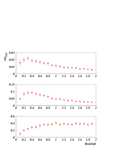
FIG. 2.: The attenuation integrated over the rest-frame $B$-band of Type Ia SNe due to photon-axion oscillations with $n_{\rm e}=10^{-7}\,{\rm cm}^{-3}(1+z)^{3}$ (upper panel), $n_{\rm e}=5\times 10^{-8}\,{\rm cm}^{-3}(1+z)^{3}$ (middle panel) and $n_{\rm e}=10^{-8}\,{\rm cm}^{-3}(1+z)^{3}$ (lower panel). All other parameter-values are given by Eq. 7.

In Fig. 3, the rest-frame $B$-band magnitude attenuation for Type Ia SNe for three different values of the intergalactic field strength is shown. Again, each point represents the average value and the error bars the dispersion for ten different lines-of-sight. In the upper panel, $B_{\rm 0}=10^{-10}(1+z)^{2}\,{\rm G}$, in the middle panel $B_{\rm 0}=5\times 10^{-10}(1+z)^{2}\,{\rm G}$ and in the lower panel $B_{\rm 0}=10^{-9}(1+z)^{2}\,{\rm G}$. All other parameter-values are given by Eq. 7.

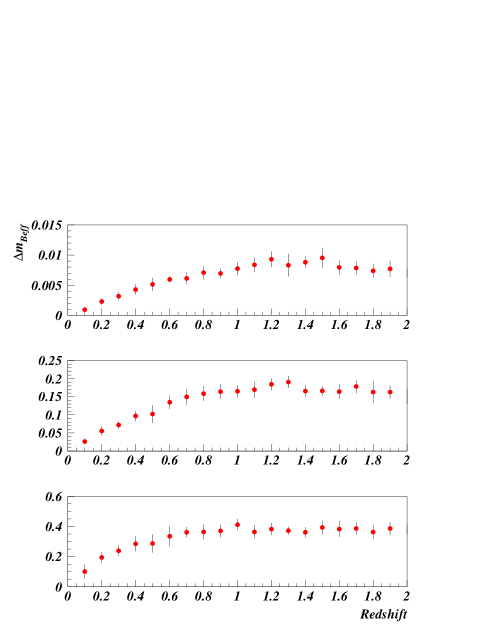
FIG. 3.: The attenuation integrated over the rest-frame $B$-band of Type Ia SNe due to photon-axion oscillations with $B_{\rm 0}=10^{-10}(1+z)^{2}\,{\rm G}$ (upper panel), $B_{\rm 0}=5\times 10^{-10}(1+z)^{2}\,{\rm G}$ (middle panel) and $B_{\rm 0}=10^{-9}(1+z)^{2}\,{\rm G}$ (lower panel). All other parameter-values are given by Eq. 7.

Our results indicate that we need low electron densities in order to get an attenuation that increases with redshift. One should keep in mind that the overall normalization can be set by varying the strength of the magnetic fields and/or the photon-axion coupling strength.

Based on a sample of 36 $z\sim 0.5$ SNe Perlmutter et al. [5] measured the the average rest-frame $B-V$ color excess to be $0.035\pm 0.022$ mag. We find the expected color excess with our standard set of parameters to be, $E(B-V)=0.006$, with a scatter around this value of 0.004 mag, as shown in Fig. 4 where we have simulated 200 Type Ia SNe at z=0.5.

FIG. 4.: Color extinctions for rest-frame $E(B-V)$ for 200 Type Ia SNe at $z=0.5$.

We can investigate the frequency dependence when doing broad-band photometry by studying the extinction (at maximum intensity) in $V-J$, $R-J$ and $I-J$ for Type Ia SNe as a function of redshift, as we show in Fig. 5. All the broad-band filters and spectroscopy wavelength scales are in the observer’s frame. We can see that in all three cases, the color excess is very small and thus difficult to measure.

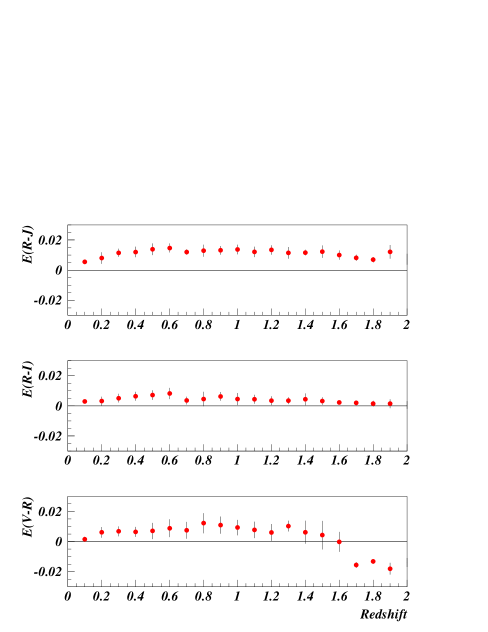
FIG. 5.: Color extinctions $E(V-J)$, $E(R-J)$ and $E(I-J)$ for Type Ia SNe as a function of redshift. Note that the dimming associated with photon-axion mixing, unlike extinction by dust, also can generate blueing.

In general, the nature of the frequency dependence will depend on the exact values of the input parameters with the possibility of generating both reddening and blueing, where in some cases the nature of the effect will depend on redshift (see, e.g., lower panel of Fig. 5). We thus conclude that it will be very difficult to use the color excess between different broad-bands to put severe limits on the photon-axion mixing parameters.

V Discussion

Our numerical simulations indicate that in order to get a dimming effect from photon-axion oscillations similar to the one from a cosmological constant (increasing at lower redshifts, saturating at higher), one would need to have an average intergalactic electron density of $n_{\rm e}\lesssim 10^{-8}\,{\rm cm}^{-3}(1+z)^{3}$. Assuming this, it should be possible to vary the average magnetic field strength or the photon-axion coupling strength in order to fit the current broad-band photometry data. Note that in the case of close to maximal mixing, results are generally not very sensitive to the exact values of the input parameters, yielding results similar to the upper panel in Fig. 2.

Depending on the choice of mixing parameters the color excess terms of sources at cosmological distances could be either positive or negative, the latter case being particularly interesting as it could not be confused with regular extinction by dust. Since photon-axion oscillations can cause either reddening or blueing (or no color excess at all) for close to maximal mixing and the integrated broad-band magnitudes wash out the dispersion in attenuation, we expect spectroscopic studies of high-z objects to be a more powerful discriminator between different oscillation models and the case of a cosmological constant or any other dark energy component (for which we suppose the dimming to be entirely frequency independent). Systematic analysis of quasar, gamma-ray burst and galaxy spectra as a function of redshift by, e.g., the Sloan Digital Sky Survey and 2dF groups are probably the best probes for the photon-axion mixing parameter space. Note that the source size sets a lower limit to the size of the fluctuations that can be probed since the fluctuations will average out if photons from different parts of the source will travel through different magnetic field strengths and electron densities.

SN spectra, available with good signal-to-noise ratios up to at least $z\sim 0.5$, are useful probes for the large mixing parameters that would yield a sufficient dimming of Type Ia SNe as to explain the Hubble diagrams in [5, 6] without invoking dark energy.

REFERENCES

- [1] C. Csaki, N. Kaloper and J. Terning, arXiv:hep-ph/0111311.
- [2] C. Deffayet, D. Harari, J. P. Uzan and M. Zaldarriaga, arXiv:hep-ph/0112118.
- [3] D. Grasso and H. R. Rubinstein, Phys. Rept. 348, 163 (2001) [arXiv:astro-ph/0009061].
- [4] C. Csaki, N. Kaloper and J. Terning, arXiv:hep-ph/0112212.
- [5] S. Perlmutter et al., Astrophys. J., 517 (1999) 565
- [6] A. G. Riess et al., Astron. J., 116 (1998) 1009
- [7] J.J. Sakurai, Modern Quantum Mechanics, Reading, 1995.
- [8] We have used the lsoda package from Netlib, http://www.netlib.org
- [9] A. Goobar, L. Bergström and E. Mörtsell Astron. & Astrophys., in press, arXiv:astro-ph/0201012.