NGC 1866: a workbench for stellar evolution

NGC 1866 is a young, rich star cluster in the Large Magellanic Cloud. Since the cluster is very well populated both in the main sequence and post main sequence stages, thus providing us with a statistically complete sample of objects throughout the various evolutionary phases of intermediate mass stars, it represents a good laboratory for testing stellar evolutionary models. More precisely, NGC 1866 can be used to discriminate among classical stellar models, in which the extension of the convective regions is fixed by the classical Schwarzschild criterion, from models with overshooting, in which an “extra-mixing” is considered to take place beyond the classical limit of the convective zone. Addressing this subject in a recent work, Testa et al. (1999) reached the conclusion that the classical scheme for the treatment of convection represents a good and sufficient approximation for convective interiors. Using their own data, we repeat here the analysis. First we revise the procedure followed by Testa et al. (1999) to correct the data for completeness, second we calculate new stellar models with updated physical input for both evolutionary schemes, finally we present many simulations of the colour-magnitude diagrams and luminosity functions of the cluster using the ratio of the integrated luminosity function of main sequence stars to the number of giants as the normalization factor of the simulations. We also take into account several possible physical agents that could alter the color-magnitude diagram and the luminosity function: they are unresolved binary stars, dispersion in the age, stochastic effects in the initial mass function. Their effect is analyzed separately, with the conclusion that binary stars have the largest impact. The main result of this study is that the convective overshoot hypothesis (together with a suitable percentage of unresolved binaries) is really needed to fully match the whole pattern of data. The main drawback of the classical models is that they cannot reproduce the correct ratio of main sequence to post-main sequence stars.

1 Introduction

In the context of stellar theories, it has long been acknowledged that the penetration of convective elements beyond the classical limit set by the Schwarzschild criterion could produce non-negligible effects on the stellar structure.

The young star cluster NGC 1866 in the Large Magellanic Cloud (LMC) is considered as an ideal laboratory for testing stellar models, especially concerning the extension of convection in the interiors of real stars, and discriminating among classical and so-called overshooting models. This cluster, well populated both in main sequence and giants stars, represents a statistically complete sample of objects, contrary to the young clusters of the Milky Way (that are relatively poor, especially in giant stars). Furthermore, NGC 1866 is young enough ($\simeq$100 Myr) to possess stars which develop a convective core in the phase of central H-burning ($M_{\rm TO}=4-5$ M_⊙), thus providing us the way to test the extension of overshooting. The theory of stellar structure predicts that convective cores in main sequence stars set in starting from initial masses greater than $M\simeq 1.1$ M_⊙. For these reasons NGC 1866 has been the subject of several analyses, aiming at testing how far convective elements overshoot from the core into the surrounding stable layers.

Becker & Mathews (1983), comparing observational and synthetic colour-magnitude diagrams (CMD) of NGC 1866, obtained the best fit to the data simulating a cluster of about $86$ Myr: the general features of the CMD were well-fitted on the whole, but the authors argued that the classical stellar models they used predicted a number of red giants larger than observed, and a smaller number of main sequence stars in turn as compared to the observations. The same authors suggested that a more careful treatment of core convection (i.e. larger convective cores) could remove the discrepancy. A number of subsequent studies confirmed this idea and demonstrated that the inclusion of overshooting in the description of convective motions could reproduce the correct ratio $N_{\rm PMS}/N_{\rm MS}$. Chiosi et al. (1989a), in particular, clearly showed that the overshooting scheme, by reducing the ratio $t_{\rm He}/t_{\rm H}$, offers a good and simple solution to the problem. This conclusion was also reinforced by Lattanzio et al. (1991), who analyzed the CMD of NGC 1866 by means of overshooting and classical models .

Over the years, sophisticated formulations of convective overshooting have been elaborated that are based on turbulence theories (Cloutman & Whitaker, 1980; Xiong, 1980) and fluid hydro-dynamics (Canuto & Mazzitelli, 1991; Canuto et al., 1996; Unno & Kondo, 1989). However, the ballistic approach at the problem proposed by Bressan et al. (1981) turns out to be fully adequate and it has been proved to best reproduce the numerical results of laboratory fluid-dynamics simulations (Zahn, 1991). The Bressan et al. (1981) algorithm adopts a non-local treatment of convection in the context of the mixing-length theory (MLT) by Böhm-Vitense (1958): it looks for the layers where the velocity of convective elements (accelerated by the buoyancy force in the formally unstable regions) becomes zero in the surrounding stable regions, then adopts a suitable temperature stratification in the overshooting regions, and finally assumes straight mixing over-there. Since the Bressan et al. (1981) formalism makes use of the MLT, it expresses the mean free path of the convective elements as $l=\Lambda_{\rm c}\times H_{\rm p}$ where $H_{\rm p}$ is the local pressure scale height.

Although some criticism has been advanced by Renzini (1987) –who erroneously concludes that the “miscellaneous” of local and non local formalisms leads to overestimating the overshooting distance– we remind the reader that overshooting is simply a logical consequence of the inertia principle, so that neglecting its existence would not be physically sound. It is worth recalling that convective overshooting is quite common in nature (Deardorff et al., 1969), and it has been demonstrated in a number of studies, including numerical simulations (Freytag et al., 1996), that the penetration depth of convective elements into a formally stable region represents a non-negligible fraction of the size of the unstable zone.

In addition to this, there are a number of astrophysical situations in which the hypothesis of substantial convective overshooting has been found to offer better and more elegant solutions than other explanations (see Bertelli et al., 1986; Chiosi et al., 1992). Among others, it suffices to recall here the so-called mass discrepancy of Cepheid stars (Bertelli et al., 1993; Chiosi et al., 1992).

Despite this, it has been often argued that unresolved binaries could mimic the effects of convective overshooting and easily account for the low ratio of red giant to main sequence stars observed in the young LMC clusters. This hypothesis has been investigated by many authors, both in open clusters of the Milky Way (see Carraro et al., 1994) and young clusters of the LMC (Chiosi et al., 1989a, b; Vallenari et al., 1992) with somewhat contrasting results.

In their study, Testa et al. (1999) emphasize the role of unresolved binaries in solving the problem, reaching the conclusion that overshooting is not needed. They obtain agreement with the observational data only by introducing a fraction of about $30\,\%$ of binary stars in a population of $\simeq 100$ Myr, and using the classical semi-convective models of Dominguez et al. (1999). In contrast, models computed with “enlarged” convective cores (i.e. cores in which convection extends beyond the Schwarzschild criterion to simulate overshooting), lead to worse fits of the observational data, especially when binary stars are included.

Unfortunately, Testa et al. (1999) adopt a wrong procedure to correct the observational star counts for photometric completeness (see the section below), thus obtaining differential ($N_{\rm MS}$, shortly indicated with DLF) and integrated luminosity functions ($\Sigma N_{\rm MS}$, shortly referred to as ILF) for the main sequence stars of NGC 1866 that are inconsistent. Furthermore, Testa et al. (1999) fail to make use of the ILF normalized to the number of evolved stars ($\Sigma N_{\rm MS}/N_{\rm PMS}$, hereinafter indicated as N-ILF) introduced by Chiosi et al. (1989a), which has been proved to be the only way to effectively discriminate between the two different evolutionary schemes. It is worth reminding the reader that the N-ILF is by definition proportional to the lifetime ratio $t_{\rm H}/t_{\rm He}$.

In this paper, first we correct the analysis of the observational data and second we show that the conclusions reached by Testa et al. (1999) entirely depend on the kind of diagnostic they have adopted. Exploring the relative effects of core overshoot and unresolved binary star frequency on intermediate age cluster CMD’s will be a side product of our analysis.

Starting from the same observational data used by Testa et al. (1999), and correctly applying the completeness correction, in this paper we shall discriminate –by means of simulated CMDs and LFs of NGC 1866– between classical semi-convective and overshooting models. After a brief description of the observational data (Sect. 2), in Sect. 3 we compare the stellar models calculated according to the two schemes, with particular attention to the values of critical masses and lifetime ratios. These latter are indeed the crucial point to test the validity of stellar models. In Sect. 4 we describe the isochrones and the methods used to simulate CMDs and LFs. In Sect. 5 we compare the results of these simulations with their observational counterparts. In Section 6 we thoroughly discuss the reasons why our conclusions differ from those by Testa et al. (1999). Finally, in Sect. 7 we summarize the main results of this study.

Figure 1: CMD for stars in the adopted sample, after statistical de-contamination (Testa et al., 1999)

2 Observational data

The observational data (Testa et al., 1999) have been obtained with the $2.2$ m ESO telescope at La Silla, Chile, on 1993 January 27. Two fields have been observed in $B$ and $V$ pass-bands: the first field is centered on the cluster, and the second one is located at $\sim 6^{\prime}$ from it. The second field is utilized for statistical field subtraction: the corrected and calibrated CMD of Testa et al. (1999) is presented in Fig. 1, in which the main sequence stars are separated from giants by dashed lines.

Table 1: Luminosity functions for main sequence stars in NGC 1866 as adopted in Testa et al. (1999): differential and integrated luminosity functions before the completeness correction (columns 2 ad 3), the completeness factors (column 4), differential and integrated luminosity functions after the completeness correction (column 5 and 6). The last three columns present the corrected luminosity functions as obtained independently by us, starting from the original Testa et al. (1999) data.

	Testa et al. (1999)					This work
(1)	(2)	(3)	(4)	(5)	(6)	(7)	(8)	(9)
$m_{\rm V}$	$N_{\rm MS}$	$\Sigma N_{\rm MS}$	$\lambda_{\rm c}$	$(N_{\rm MS})_{\rm corr}$	$\Sigma(N_{\rm MS})_{\rm corr}$	$N_{\rm MS}$	$(N_{\rm MS})_{\rm corr}$	$\Sigma(N_{\rm MS})_{\rm corr}$
16.5	0	0	1.000	0	0	3	3	3
16.7	2	2	1.000	2	2	3	3	6
16.9	9	11	1.000	9	11	10	10	16
17.1	17	28	1.000	17	28	20	20	36
17.3	37	65	1.000	37	65	37	37	73
17.5	29	94	1.000	29	94	33	33	106
17.7	56	150	1.000	56	150	59	59	165
17.9	55	205	1.000	55	205	61	62	227
18.1	69	274	0.996	69	275	74	74	301
18.3	90	364	0.992	90	367	84	85	386
18.5	116	480	0.988	117	486	129	131	517
18.7	135	615	0.981	137	627	144	146	663
18.9	160	775	0.975	163	795	167	172	835
19.1	164	939	0.966	168	972	174	180	1015
19.3	188	1127	0.958	194	1177	208	217	1232
19.5	215	1342	0.950	222	1413	227	238	1470
19.7	266	1608	0.939	279	1712	276	292	1762
19.9	250	1858	0.929	263	2001	256	274	2036
20.1	274	2132	0.916	292	2327	274	297	2333
20.3	323	2455	0.903	352	2720	313	346	2679
20.5	303	2758	0.889	332	3101	316	351	3030
20.7	322	3080	0.874	355	3524	299	334	3364
20.9	302	3382	0.859	336	3939	295	331	3695
21.1	290	3672	0.842	323	4362	282	318	4013
21.3	316	3988	0.823	358	4843	289	332	4345
21.5	261	4249	0.803	299	5290	238	278	4623
21.7	86	4335	0.776	100	5587	88	106	4729
21.9	16	4351	0.744	29	5850	36	50	4779

2.1 Correction for completeness

In their analysis, Testa et al. (1999) divide the sample in six concentric rings centered on the cluster, and calculate the completeness factors, $\lambda^{i}_{\rm c}$, ring by ring. Since $\lambda^{i}_{\rm c}$ is equal to the number ratio of artificial stars added and recovered in a given magnitude bin, they should be used to correct the DLF – i.e. the number of stars per magnitude bin – separately for each ring $i$:

$$(N^{i})_{\rm corr}=N^{i}/\lambda^{i}_{\rm c}$$ (1)

where $N^{i}$ and $(N^{i})_{\rm corr}$ stand for the observed and corrected numbers, respectively.

However, a substantial error is made by Testa et al. (1999): they use the same $\lambda_{\rm c}$ factors to correct both the number of stars and the ILF at each magnitude bin. This clearly produces the correct DLF $(N^{i})_{\rm corr}$, but over-estimates the ILF and N-ILF at fainter magnitude bins. This can be appreciated by looking at the first 6 columns of Table 1, where we present the original star counts and the luminosity functions used by Testa et al. (1999). In particular, it can be noticed that, starting from the uncorrected DLF and ILF of columns 2 and 3, the same “average” $\lambda_{\rm c}$ factors (column 4) have been used to derive the corrected DLF shown in column 5 (i.e. $(N_{\rm MS})_{\rm corr}=N_{\rm MS}/\lambda_{\rm c}$), and the corrected ILF shown in column 6 (i.e. $\Sigma(N_{\rm MS})_{\rm corr}=\Sigma N_{\rm MS}/\lambda_{\rm c}$). The corrected DLF and ILF obtained in such a way are no longer consistent with each other.

Noticing this, we decided to completely re-derive the luminosity functions for NGC 1866, starting from the statistically decontaminated photometric data of Testa et al. (1999) (see Fig. 1), and the completeness factors presented in their Fig. 6. In short, we have obtained the DLF for each annulus around NGC 1866, and corrected them using the corresponding completeness factors separately, according to Eq. (1). Then, the DLFs for annulus 2 to 5 were added

$$(N_{\rm MS})_{\rm corr}=\sum_{i=2}^{5}(N^{i}_{\rm MS})_{\rm corr}$$ (2)

producing the total DLF presented in column 8 of Table 1. (For the sake of comparison, column 7 of the same table presents the counts obtained by adding stars from annulus 2 to 5, without applying the completeness correction.) ¿From this corrected DLF we derive the total ILF of column 9 of the same table, by simply summing up the number of stars above each magnitude bin. As can be readily seen, our final numbers for the DLF are roughly consistent with those of Testa et al. (1999), but the two ILFs are sizeably different, especially for the faintest magnitude bins.

There is a final remark to be made for the sake of clarity. Comparing columns (2) and (7), which contain the rough counts in the various magnitude bins, a marginal disagreement is evident: our counts do not exactly coincide with those by Testa et al. (1999). The difference is due to the slightly different criteria adopted to define the numbers $N_{MS}$ of stars per magnitude interval. Testa et al. (1999) follow a complicated scheme in which (i) the mean location of the MS together with its color dispersion $\sigma$ are derived as a function of the magnitude, and (ii) in every magnitude bin only stars falling within 7$\sigma$ from the mean MS are taken into account. In contrast, we prefer to consider all stars falling within the considered magnitude interval. As a consequence of this, the $N_{MS}$ of Testa et al. (1999) are slightly smaller than ours because stars far away from the mean MS are neglected.

In Fig. 2 we compare our results for the corrected ILF (continuous line) with those obtained by Testa et al. (1999) (dashed line). It is important to stress here that one of reasons why our results differ from those by Testa et al. (1999), resides in the different (and erroneous) way of applying the completeness corrections used by them.

Figure 2: Integrated Luminosity Function of the main sequence stars of NGC 1866 before (dotted lines) and after (thick line) correcting for photometric completeness. The dashed line shows the same luminosity function calculated by Testa et al. (1999)

Finally, we summarize in Table 2 the total number of main sequence ($\Sigma N_{\rm MS})$ and post main sequence ($N_{\rm PMS})$ stars before and after the completeness correction is applied. The number of post main sequence stars amounts to $N_{\rm PMS}=100$.

3 Stellar tracks

We have calculated two sets of stellar tracks with the classical semi-convective scheme and initial chemical composition [$Y$=0.240,$Z$=0.004] and [$Y$=0.250,$Z$=0.008], and one set of models with convective overshooting and composition [$Y$=0.240,$Z$=0.004]. The initial masses of the models range from $1.0$ to $8$ M_⊙. The input physics is the same as in Girardi et al. (2000) and subsequently updated by Salasnich et al. (2000), to whom the reader should refer for all details. For purposes of comparison, whenever required we also utilize the stellar models by Salasnich et al. (2000) calculated with overshooting and chemical composition [$Y$=0.250,$Z$=0.008].

Table 2: Star counts for main sequence ($\Sigma N_{\rm MS}$) and post main sequence stars ($N_{\rm PMS}$), before and after completeness correction.

	$\Sigma N_{\rm MS}$	$N_{\rm PMS}$
observed	4395	100
corrected	4779	100

3.1 Prescriptions for semi-convection and overshooting

The algorithm dealing with semi-convection in classical models strictly follows the recipes given by Alongi et al. (1993) to whom the reader should refer for all details.

Convective overshooting is based on the formulation by Bressan et al. (1981) and the more recent revision by Bertelli et al. (1985) and Alongi et al. (1993). Suffice it to recall here that the overshooting parameter $\Lambda$ is chosen to be $\Lambda_{\rm c}$=0.5 for core convection and $\Lambda_{\rm e}$=0.7 for envelope convection (see Alongi et al., 1993).

For the sake of clarity and to avoid misunderstanding, we remind the reader that $\Lambda_{\rm c}$=0.5 in the formalism of Bressan et al. (1981) is equivalent to $\Lambda_{\rm c}$=0.25 in the description of Maeder & Meynet (1991). More precisely, while Bressan et al. (1981) define the overshooting distance as the path traveled by a convective element across the Schwarzschild border (half distance beneath and half above the border), Maeder & Meynet (1991) define it only as the distance above the border. Furthermore, the choice of $\Lambda_{\rm c}$=0.5 we have adopted is the same as in previous studies aimed at generating stellar models best suited to interpret observational data of star clusters. To mention a few we recall Alongi et al. (1993), Bressan et al. (1993), Maeder & Meynet (1991), Meynet et al. (1994), Chiosi et al. (1992), Chiosi (1999) and references therein. Exploring the effects of core overshooting for other choices of $\Lambda_{\rm c}$ is beyond the scope of this study.

Figure 3: The stellar tracks for the $2.5$ e $4$ M_⊙ stars with composition [$Y$=0.250, $Z$=0.008]. The solid lines are the stellar models with convective overshooting, whereas the dotted lines are the models with the classical extension of the convective core

3.2 Critical masses $M_{\rm HeF}$, $M_{\rm up}$

As long ago pointed out by Chiosi et al. (1989a), see also Chiosi et al. (1992), in the presence of core overshooting the minimum initial masses, below which core He-flash and core C-ignition in highly degenerate material occur, $M_{\rm HeF}$ and $M_{\rm up}$ respectively, get smaller. Table 3 summarizes the results obtained for classical semi-convective and overshooting models with metallicity $Z$=0.004 and $Z$=0.008. The same result holds good for both values of $Z$.

Table 3: Critical masses $M_{\rm HeF}$ e $M_{\rm up}$ – in units of M_⊙ – for classical semi-convective and overshooting models.

	$M_{\rm HeF}$	$M_{\rm up}$
classical	$2.2-2.5$	$>8$
overshooting	$1.8-2.0$	$\simeq 7$

Table 4: Lifetimes for classical models with chemical composition [$Y$=0.250,$Z$=0.008]. The lifetimes are in Gyr.

$M/M_{\odot}$	$t_{\rm H}$	$t_{\rm He}$	$t_{\rm He}/t_{\rm H}$
2.5	0.4094	0.2436	0.595
3.5	0.1769	0.1293	0.389
4.0	0.1271	0.0688	0.340
5.0	0.0775	0.0219	0.283
6.0	0.0524	0.0126	0.241
7.0	0.0385	0.0079	0.208
8.0	0.0299	0.0056	0.189

Table 5: The same as in Table 4 but for the overshooting models.

$M/M_{\odot}$	$t_{\rm H}$	$t_{\rm He}$	$t_{\rm He}/t_{\rm H}$
2.5	0.5438	0.1376	0.253
3.5	0.2308	0.0380	0.165
4.0	0.1674	0.0237	0.141
5.0	0.0999	0.0116	0.116
6.0	0.0672	0.0065	0.096
7.0	0.0487	0.0043	0.090
8.0	0.0376	0.0032	0.085

3.3 Lifetimes and lifetime ratios

Because of the increased size of the convective cores, the central H-burning lifetime $t_{\rm H}$ in the overshooting models is $30\,\%$ longer than in classical ones, this effect depending on the parameter $\Lambda_{\rm c}$ (Bressan et al., 1981). The “over-luminosity” caused by overshooting during the core H-burning phase (see Fig. 3) still remains during the He-burning phase (for stars with initial mass greater than $M_{\rm HeF}$): consequently, the lifetime of the He-burning phase ($t_{\rm He}$) gets shorter by about $40-45\,\%$. This, combined with the longer $t_{\rm H}$, results in a strong decrease ($\sim 55-60\,\%$) of the ratio $t_{\rm He}/t_{\rm H}$. Tables 4 and 5 summarize the lifetimes for some of the $Z$=0.008 models calculated with the classical and overshooting scheme, respectively.

4 Isochrones and synthetic CMDs

4.1 Isochrones

For the above four groups of evolutionary tracks, we have derived the isochrones, adopting the algorithm of “equivalent evolutionary points” developed by Bertelli et al. (1994). The age ranges from about $0.05$ to $10$ Gyr. Isochrones are calculated at $\Delta\log t=0.01$ intervals: this means that any two consecutive isochrones differ by $\sim 2\,\%$ in their ages. Along each isochrone we give: the initial and actual stellar masses, the logarithm of surface luminosity, the effective temperature and surface gravity, the absolute bolometric magnitude, and the absolute magnitudes in the $UBVRIJHK$ pass-bands. Finally we list the indefinite integral over the initial mass $M$ of the initial mass function (IMF). For any other detail see Girardi et al. (2000).

Theoretical luminosities and effective temperatures are translated into magnitudes and colours in the Johnson-Cousins system, using the conversions of Bertelli et al. (1994), which provides colours and bolometric corrections as a function of the effective temperature and gravity. The Bertelli et al. (1994) conversions are based on the library of synthetic spectra obtained from theoretical models of stellar atmospheres by Kurucz (1992).

We only note here, as illustrated in Fig. 4, that an isochrone of the overshooting scheme runs at higher luminosities as compared to a “classical” isochrone of the same age, that is, in the presence of overshooting isochrones of older ages are required to fit the observational data of a cluster.

Figure 4: Isochrones of same age ($200$ Myr) and chemical composition, [$Y$=0.250,$Z$=0.008] calculated with classical (dashed line) and overshooting models (solid line)

4.2 Synthetic CMDs

The synthetic CMDs are constructed by means of a Monte Carlo algorithm, which randomly distributes stars along a given isochrone according to evolutionary lifetimes and IMF. The code takes into account the photometric errors affecting the observational data (derived from Testa et al. (1999) tables), by adding an artificial dispersion to the theoretical magnitudes and colours, and generates numerical simulations of CMDs allowing for effects due to: age spread of the cluster population, different slopes of the IMF, and presence of a certain fraction of unresolved binary stars with mass ratio ranging in a given interval.

Since any plausible IMF preferentially populates the main sequence region of an isochrone, in order to reproduce the right proportion of main sequence to post main sequence stars –according to the lifetimes in the various evolutionary phases– we populate our synthetic CMDs until an assigned number of post main sequence stars $N_{\rm PMS}$ is matched: in particular in each simulation presented here, we impose that the total number of red giant stars present in the data is matched. In such a way $N_{\rm PMS}$ is taken as the “normalization” parameter of the simulations (see Chiosi et al., 1989a; Vallenari et al., 1991; Lattanzio et al., 1991).

4.3 Luminosity functions

Special care is paid to the integrated number of stars from the tip of main sequence band down to the current magnitude interval, normalized to the number of red giant stars (i.e. the N-ILF). As pointed out by Chiosi et al. (1989a), the N-ILF can be directly compared with the ratio of lifetimes in the core H- and He-burning phases, $t_{\rm H}$ and $t_{\rm He}$, respectively. At fixed $N_{\rm PMS}$, the ratio in each simulation $\Sigma N_{\rm MS}/N_{\rm PMS}$ depends on the age –an older population clearly has a larger $N_{\rm PMS}$– and the theoretical model in use. As already noted in previous sections, the size of the convective cores strongly affects the ratio $t_{\rm He}/t_{\rm H}$, and in turn, the ratio $\Sigma N_{\rm MS}/N_{\rm PMS}$. Thus the N-ILF, when compared to the observational counterpart, reliably discriminates classical from overshooting models.

Concluding this section, it is worth remarking that reproducing synthetic CMDs with an assigned number of post main sequence stars is by far preferable to simulating CMDs with a fixed total number of stars brighter than a certain magnitude. As a matter of fact, the distribution of stars along the main sequence is driven almost exclusively by the IMF, evolutionary effects playing only a marginal role. Therefore, the LF (either DLF or ILF) of the main sequence stars, if not normalized to the number of giants, would only reflect the underlying IMF, and would not be affected by the effects of overshooting we want to test.

5 The simulations

In this section we present the CMDs and LFs resulting from our simulations, and compare them with the observational ones, both for classical semi-convective and overshooting models.

5.1 Adopted parameters

Before presenting the simulations, we briefly summarize the values adopted for parameters such as reddening, metallicity, and distance modulus.

5.1.1 IMF

All the simulations are calculated adopting the Salpeter (1955) law $dN\propto M^{-\alpha}dM$ for the IMF and assuming, unless otherwise specified, the parameter $\alpha=2.35$.

5.1.2 Metallicity

Rough estimates of the metallicity of NGC 1866 derived from the $BVI_{\rm c}$ colors of the Cepheids (Caldwell & Coulson, 1985; Feast, 1989) yield [Fe/H]$=-0.1\pm 0.3$ (see also Bertelli et al., 1993), finally the recent analysis by Testa et al. (1999) yielded [Fe/H]$\simeq-0.35$. This roughly corresponds to $Z=0.009$. Therefore, improving upon the metallicity used in the old studies by Chiosi et al. (1989a) and Brocato et al. (1989) who adopted isochrones with [$Y$=0.280,$Z$=0.020] in the present simulations we assume the composition [$Y$=0.250,$Z$=0.008].

5.1.3 Distance modulus

The distance modulus to the LMC is a hotly debated issue: we summarize here some of the most recent determinations of this parameter. Cepheid stars with Hipparcos parallaxes indicate $(m-M)_{\rm 0}\sim 18.6$ (Feast, 2000). The analysis of the expanding ring around SN1987A yields $(m-M)_{\rm 0}=18.58\pm 0.05$ (Panagia, 1998). The simultaneous study of the Cepheids stars and CMD of NGC 1866 by Bertelli et al. (1993) yields $(m-M)_{\rm 0}=18.51\pm 0.21$ In a recent study on young LMC clusters Keller et al. (2000) utilize the value $(m-M)_{\rm 0}=18.45$. We adopt here $(m-M)_{\rm 0}=18.5$, as the “classical” value for the LMC distance modulus (Westerlund, 1997). Passing from $(m-M)_{\rm 0}=18.5$ to $(m-M)_{\rm 0}=18.6$ would not significantly change the results of the present analysis.

5.1.4 Reddening

The study of the dust distribution across the LMC by means of photometric and spectroscopic data gives reddening maps from which one derives an estimate of the mean value $E_{B-V}=0.16$ (Oestreicher & Schmidt-Kaler, 1996), with a maximum value of 0.29 (reached in the region of 30 Dor) and a minimum of 0.06 (Zaritsky et al., 1997). While Testa et al. (1999) assume $E_{B-V}$ in the range between $0.06$ to $0.10$, we prefer to adopt the value $0.10$ which, taking the total visual extinction $A_{V}$ to be $3.1\times E_{B-V}$ (Rieke & Lebofsky, 1985), corresponds to $A_{V}=0.31$.

5.2 Classical semi-convective models

In Fig. 5 is shown a synthetic CMD for the age of 76 Myr, and turn-off mass $M_{\rm TO}=5M_{\odot}$. The termination magnitude of the main sequence band fits the observational data. However, the luminosity interval spanned by the blue loop does not agree with the observed CMD. Theoretical luminosities are indeed brighter than observed. Contrary-wise, if we impose that the mean luminosity of red giants is matched, the age increases to $110$ Myr but the observational termination magnitude of the main sequence is about $1$ mag brighter than the theoretical one. In Fig. 6 we present the comparison between the observational (dashed line) and the theoretical N-ILF (solid line) for the population of $76$ Myr in Fig. 5. The stellar models in use yield a ratio $\Sigma N_{\rm MS}/N_{\rm PMS}$ lower than the observational one. Since $N_{\rm PMS}$ is taken equal to the number of red giants detected in NGC 1866, this implies that the classical semi-convective models produce more giants than observed (a long known result).

Figure 5: Synthetic CMD constructed with classical models. The age is $76$ Myr, the chemical composition is [$Y$=0.250,$Z$=0.008].

Figure 6: Observational (dashed line) N-ILF —with the poissonian error bars— and theoretical N-ILF (thick line) for the case of classical models shown in Fig. 5. The age is of $76$ Myr and the chemical composition is [$Y$=0.250,$Z$=0.008]

Figure 7: Synthetic CMD for the age of $160$ Myr, obtained from models with overshooting and chemical composition [$Y$=0.250,$Z$=0.008]

Figure 8: Observational (dashed line) N-ILF —with the poissonian error bars— and theoretical N-ILF (thick line) for the case of $160$ Myr shown in Fig. 7

5.3 Models with overshooting

As already anticipated commenting Fig. 4, the longer lifetime and brighter luminosities of stellar models with overshooting impose older isochrones to be adopted in the CMD simulations. Figs. 7 and 8 illustrate the synthetic CMD and the N-ILF, respectively, and compare them with their observational counterparts for a population $160$ Myr old and turn-off mass of $M_{\rm TO}=4.1M_{\odot}$. Although a larger ratio $\Sigma N_{\rm MS}/N_{\rm PMS}$ is obtained as compared with the classical case, still the agreement between theory and observations is not fully satisfactory: indeed, while the region of the blue loop is well fitted, the main sequence termination magnitude is about $1$ mag fainter than observed.

Alternatively, if a younger age ($\simeq 100$ Myr) is adopted to match the main sequence termination luminosity, theory and observations would disagree in the morphology of the blue loop. Furthermore, it would predict too a high number of main sequence stars ($\Sigma N_{\rm MS}\simeq 10000$) compared to the observed number of red giants ($N_{\rm PMS}=100$), i.e. the ratio $\Sigma N_{\rm MS}/N_{\rm PMS}$ would be too high.

5.4 Including binary stars

The effect of unresolved binary stars (UBS) on the CMD of stellar clusters has been investigated in a number of studies (see Chiosi et al., 1989a; Vallenari et al., 1991).

The main effect of UBS on the main sequence morphology would be the appearance of a second sequence, running parallel to the main sequence, but systematically cooler and with brighter luminosities ($\simeq 0.7$ mag for binary stars of equal mass). It goes without saying that in order to detect this secondary sequence the number of UBS must be significant.

The percentage of UBS in open clusters of the Milky Way seems to amount to about 30 % – 50 % of the cluster population (Mermilliod & Mayor, 1989; Carraro et al., 1994). Likely the same percentage of UBS could exist also in young clusters of the LMC. Strong observational evidence of this comes from the recent study of Elson et al. (1998) on NGC 1818, a young cluster similar to NGC 1866. In the CMD obtained with $HST$ data, the existence of a “double” main sequence is soon evident. Elson et al. (1998) explain this feature by supposing the existence of a population of UBS amounting to 30–35 % of the total and with mass ratios in the range $0.7$ to $1$. Systems with mass ratios different from these cannot be excluded. In any case they would be hardly distinguishable from single objects.

Basing on the study by Elson et al. (1998), we include in our simulations the same fraction of binary stars, to understand how they alter the above conclusions both for classical and overshooting models. Unless otherwise specified, the mass ratio $q$ of the UBS included in the simulations falls in the interval $0.7<q<1$ in agreement with Elson et al. (1998).

The presence of UBS, shifting the main sequence termination toward brighter luminosities, requires older ages. At the same time, the older the isochrone, the fainter is the blue loop. Therefore, under the action of the two effects, the luminosity gap between the main sequence termination and red giants is reduced and the overall morphology of the CMD is better reproduced.

Figure 9: Synthetic CMD constructed with classical models, chemical composition [$Y$=0.250,$Z$=0.008], and presence of UBS. The age is $105$ Myr; the percentage of UBS amounts to $30\,\%$

Figure 10: Observational N-ILF (dashed line) —with the poissonian error bars— and theoretical ILF (thick line) for the case shown in Fig. 9: classical models, age 105 Myr, and $30\,\%$ of UBS.

5.4.1 Binary stars in the classical picture

In Fig. 9 we present the synthetic CMD for the age of $105$ Myr (turn-off mass $M_{\rm TO}=4.3$ M_⊙), in which $30\,\%$ of UBS are included. Compared to the results obtained simulating only single stars, the agreement with the observed CMD has much improved, but the theoretical N-ILF (the thick line in Fig. 10), clearly suffers the same difficulty already encountered neglecting the effects of binary stars, i.e. too low a ratio $\Sigma N_{\rm MS}/N_{\rm PMS}$. The same simulation has been repeated adopting the same percentage of binaries ($30\,\%$) but supposing that the mass ratio is distributed according to a Gaussian curve, as suggested by Testa et al. (1999). No significant difference is noticed both in the CMD morphology and N-ILF.

5.4.2 Initial mass function

How do the above results depend on the particular slope ($\alpha=2.35$) adopted for the Salpeter IMF? To cast light on this topic we have repeated our simulations varying $\alpha$ and keeping constant all other parameters. The analysis shows that while the CMD morphology is scarcely affected, the N-ILF is sensitive to variations of $\alpha$. As illustrated in Fig. 11, the N-ILF gets steeper at increasing $\alpha$. We note that, in order to reach agreement between observational and theoretical N-ILFs using the classical semi-convective models, one should adopt $\alpha$=(3.5 – 4), This would favor the formation of low mass stars still located on the main sequence. The problem is whether or not such high values of $\alpha$ are acceptable. The present results re-confirm what already pointed out in the earlier studies by Becker & Mathews (1983) and Chiosi et al. (1989a).

Figure 11: Comparison between the observational N-ILF (dashed line) and the theoretical ones (thick lines) obtained in the classical picture for a population of $105$ Myr and three different slopes for the Salpeter IMF, namely $\alpha=3,\alpha=3.5,\alpha=4$. The initial chemical composition, [$Y$=0.250,$Z$=0.008], the number of post main sequence stars ($N_{\rm PMS}=100$), and the fraction of binaries present in the sample ($30\,\%$) are constant in the three simulations

Figure 12: Synthetic CMD for overshooting models: age of $148$ Myr $30\,\%$ of UBS, and chemical composition [$Y$=0.250,$Z$=0.008]

Figure 13: Observational N-ILF (dashed line) –with the Poissonian error bars– and theoretical N-ILF (thick line) for the $148$ Myr old population shown in Fig. 12: overshooting models and $30\,\%$ of UBS

5.4.3 Binary stars in the overshooting picture

The synthetic CMD presented in Fig. 12 refers to stellar models with convective overshooting and simulates a population $148$ Myr old (turn-off mass $M_{\rm TO}=4.2$ M_⊙) containing $30\,\%$ of UBS. We note that the luminosity gap between the red giant region and the main sequence termination has now disappeared. The CMD of NGC 1866 is perfectly reproduced. The most important result is, however, the N-ILF shown in Fig. 13, which fully agrees with the observations. In other words, the ratio $\Sigma N_{\rm MS}/N_{\rm PMS}$ predicted by stellar models with convective overshoot together with the presence of a certain fraction of binary stars fully agrees with that obtained from star counts.

Figure 14: Mean N-ILF (thick line) and related $2\sigma$ levels of expectancy (dotted lines) resulting from 100 simulations of the same population including $30\,\%$ of UBS. The chemical composition is [$Y$=0.250,$Z$=0.008]. With the classical scheme (top panel) and age of 105 Myr the observational N-ILF (dashed line) is steeper than the theoretical one; for the overshooting scheme (bottom panel) and age of 148 Myr, the observational N-ILF lies inside the $\pm 2\sigma$ range around the theoretical prediction

5.5 Effects of stochastic fluctuations in the IMF

The discussion of the ILF we have presented so far, refers to a particular simulation of the CMD, which does not explicitly take into account possible effects of stochastic nature caused by the finite number of stars in a cluster. It is worth recalling here that the concept itself of IMF allows for important fluctuations to occur around the ideal distribution of stars as a function of the mass. The problem may be particularly severe for $N_{\rm PMS}$ which in most cases is a small number. In other words the question to be addressed is whether stochastic effects may change $N_{\rm PMS}$ with respect to $\Sigma N_{\rm MS}$ or conversely, whether $N_{\rm PMS}$ which has been used as the key constraint to our simulated CMDs and ILFs is generated by a unique population of main sequence stars or if many others are equally eligible.

To cast light on this issue, we have performed many simulations of our reference CMD keeping constant all parameters and letting the stochastic nature of the IMF develop thanks to the Monte Carlo technique we have adopted. To this aim, 100 simulations of the same CMD are calculated in order to get the mean N-ILF and its standard deviation $\sigma$.

For the sake of brevity, we illustrate here the results only for the cases of classical models (Fig. 14a) and overshooting models (Fig. 14b), in which $30\,\%$ of binary stars are included. No variations to the previous conclusions seem to appear. With classical semi-convective models the observed N-ILF (dashed line) runs above the $\pm 2\sigma$ interval (dotted lines) around the mean N-ILF (thick line). In contrast, with the overshooting models theoretical and observational N-ILFs agree at the $\pm 2\sigma$ level. Considering the errors affecting the observational N-ILF, the agreement is extremely good.

5.6 Age dispersion

There is a final effect to be considered, i.e. the possibility that stars in the cluster are born over a finite time interval, i.e. that a significant age spread exists.

Starting from our best-fit CMD, obtained from overshooting models with age of $\simeq 148$ Myr and including $30\,\%$ of binary stars, adding an age spread of about $20$ Myr (about 10 %) would further improve the CMD, especially in the region of red giant stars. This final CMD is presented in Fig. 15b, and compared with that of NGC 1866 (Fig. 15a). This small spread in the age while giving the final make-up of the CMD does not affect the N-ILF, and the picture outlined in Fig. 14b still holds.

Figure 15: Comparison between the CMD of NGC 1866 (Testa et al., 1999) (top panel) and our best-fit case (bottom panel), characterized by stellar models with convective overshooting, age in the interval 140–160 Myr, $30\,\%$ of UBS. The initial chemical composition is [$Y$=0.250,$Z$=0.008]. The intrinsic distance modulus is $(m-M)_{\rm 0}=18.5$.

5.7 Major uncertainties

Looking at CMD of Figs. 15b and 15a, we see that while overall agreement is reached especially as far as the magnitudes and colors of the main sequence stars, and the mean luminosity of the stars in the blue loop are concerned, there is still a marginal disagreement in the colour range spanned by the red giant stars, i.e. the extension of the blue loop. This, however, is known to depend on several factors: (i) the overshooting parameters $\Lambda_{\rm c}$ assumed for the nuclear region (see Chiosi et al., 1989a) and the one adopted for the envelope, $\Lambda_{\rm e}$ (see Alongi et al., 1991); (ii) the rate of the nuclear reaction ${}^{12}{\rm C}(\alpha,\gamma)^{16}{\rm O}$ –which determines the abundances of ${}^{12}{\rm C}$ and ${}^{16}{\rm O}$ at the end of central He-burning phase– the higher the rate, the bluer the loop (Bertelli et al., 1985). It is worth noting, however, that these uncertainties on the extension of the blue loop do not affect the star counts at the base of the ILF.

On the observational side, apart from photometric errors, completeness correction, and fraction of UBS that have already been taken into account, one has to check whether the results could depend in a crucial way on the particular calibration adopted to convert luminosities and effective temperatures into magnitudes and colours of the $UBVRI$ system. To clarify this point, we have also used the empirical conversions by Alonso et al. (1999), who present tabulations of colours and bolometric corrections as a function of the effective temperature and metallicity [Fe/H] of the stars. However, comparing isochrones calculated with this transformation and those obtained with the Bertelli et al. (1994) no appreciable difference is noticed.

Some uncertainty could be related to the particular choice for the percentage of UBS ($30\,\%$) and their mass ratios $0.7<q<1$ we have adopted. How could a change in these parameters affect our conclusions? To cast light on the issue we have performed additional simulations with different percentages and mass ratios. Increasing the binary fraction up to about $40\,\%$, and extending the mass ratio interval down to $0.5-0.6$, the CMD and N-ILF are still in agreement with the cluster data. However, assuming an even larger percentage of binary stars ($>40-45\,\%$), the CMD gets worse as the main sequence band spreads too much toward red colors.

6 Why do we disagree with Testa et al. (1999)?

The results of our analysis wholly disagree with those by Testa et al. (1999), despite the fact that we are using the same observational data for NGC 1866. Their main conclusion is indeed that classical stellar models without overshooting fit the CMD and ILF of NGC 1866 at the age of 100 Myr provided that a population of binary stars amounting to about $30\,\%$ of the total is included. In contrast our main conclusion is that even including the same percentage of binary stars only models with overshooting simultaneously reproduce the CMD, the ILF, and the correct ratio $\Sigma N_{\rm MS}/N_{\rm PMS}$. The age now is about 150 Myr.

What is the cause of the opposite conclusions? There are several factors concurring to the final result:

(i) The different procedure applied to correct star counts for photometric completeness. The ILF of Testa et al. (1999) is over-estimated due to the the fact that instead of summing up the DLF corrected for completeness in every magnitude bin, they apply the correction procedure to every step of the ILF.

(ii) The different normalization procedures of the simulations. In the present study, the normalization parameter of the simulated CMD and ILF is the total (observed) number of red giants $N_{\rm PMS}$. It is worth recalling that the N-ILF is given by $\Sigma N_{\rm MS}/N_{\rm PMS}$. The advantage of this type of normalization has already been explained by Chiosi et al. (1989a) and briefly summarized in previous sections. In contrast Testa et al. (1999) assume that each simulation is complete as soon as a given total number of stars with magnitude brighter than $M_{V}=2.6$ is reached. They justify this choice by saying that their main sequence is well defined and complete up to three magnitudes fainter than the turn-off, and assume the total number of stars observed in this magnitude interval as the normalization parameter of the simulations instead of the giant (post main sequence) stars.

(iii) This choice of the normalization factor is, however, not physically sound because a deeply observed, well populated main sequence does not tell much about the inner structure, evolutionary rates, lifetimes etc. of its stars. Indeed the distribution of the stars along the main sequence almost exclusively depends on the IMF. Therefore, the choice of a “normalization parameter” insensitive to the size of the convective core simply precludes all chances of discriminating between the two evolutionary schemes under examination. Simulations of CMDs and ILFs based on this criterion may fail to reproduce the correct ratio $\Sigma N_{\rm MS}/N_{\rm PMS}$.

(iv) In relation to this, is also the fact that the total number of stars brighter than $M_{V}=2.6$ on which the simulations are normalized is determined by the procedure of correcting for photometric incompleteness. We have already argued that the Testa et al. (1999) method is inconsistent, and overestimates the total number of stars in the main sequence. Since their simulated CMDs and ILF do actually depend on this parameter, there is no way of becoming aware of the internal inconsistency.

Considering all the differences between the present and Testa et al. (1999) analyses, we should recognize that the contrasting results are mainly due to the different way of normalizing the ILF: we choose a normalization factor (number of giants) that is sensitive to overshooting, whereas Testa et al.’s (1999) choice (stars brighter than $M_{V}=2.6$) is essentially insensitive to this effect. In fact, no clear discrimination between classical and overshooting models is expected with the latter method.

(v) To better understand this point of controversy we have repeated our simulations strictly following the procedure described by Testa et al. (1999): each one contains the same total number of stars brighter than $V=22$ as the observational data, i.e. 4879. The results are displayed in Fig. 16, limited to the few cases we have already examined. The layout of Fig. 16 is organized in vertical and horizontal groups of panels. Panels in the same vertical row correspond to the case as indicated by the top heading of the row. Panels in horizontal rows show different types of LFs as indicated: the DLF in the bottom, the total ILF (main sequence and giant stars) in the middle panels, and the ILF for the sole main sequence stars in the top panels. The results can be commented as follows:

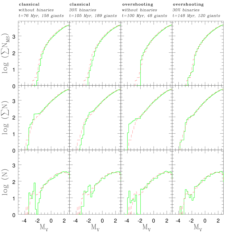
Figure 16: Summary of the four cases under consideration: the heading of each column lists the type of stellar model (classical or overshooting), the percentage of unresolved binaries, the age, and the number of giant stars. The three horizontal rows display the LFs as shown in Testa et al. (1999): the top row is the integrated LF for the sole main sequence stars in the simulation, the middle row is the integrated LF for all stars in the simulation, finally the bottom row is the DLF for the whole sample. In each panel the solid line is the theoretical LF or DLF, whereas the dashed line is the same but for the observational data. Each simulation contains a total number of stars brighter than $V=22$ equal to $4879$

• The DLFs in the bottom horizontal row make evident the luminosity gap between the main sequence termination and the giant stars, located at $M_{V}\simeq-2$. On the observational side, the gap is almost invisible, whereas on the theoretical side, the inclusion of binaries wipes out the gap in both classical and overshooting models. All models seem to reproduce the main sequence part of the DLF ($M_{V}\ga-1$) equally well.

• The total ILFs, i.e. inclusive of the post main sequence stars, are shown in the central horizontal row. For the models without binaries, the luminosity interval between the main sequence termination and the giant stars appears as a plateau in the ILF at $M_{V}\simeq-2$. To the left of this plateau, the detailed shape of the ILF is determined mainly by the location of giant stars: a slight over luminosity of the giants (with respect to observations) causes an apparent excess of stars at $M_{V}<-2$, which can be noticed in the cases of classical models with and without binaries, and overshooting models without binaries. In the case of overshooting models with binaries, giant stars are predicted at the right magnitude level, and no such discrepancy can be noticed in the ILF.

  But it is important to notice that the “excess” suggested by the ILF does not necessarily correspond to a real excess of evolved stars. This is evident if we look at the total number of giants in each simulation (see the labels at the top of the figure): in the case of classical models there is a real excess of giants (158 and 189 depending on whether or not binaries are included), which has no observational counterpart. The situation is the opposite for models with convective overshoot and no binary stars. Now the simulated number of giants is 48 (about half of what observed). Finally, models with overshooting and binaries predict the correct number of post main sequence stars (120, to be compared with the 100 observed).

• The ILF of main sequence stars (top horizontal row) does not show substantial differences passing from one case to another. This simply reflects the constancy of the IMF. There are small differences at the turn-off level, however too small to be significant.

¿From the plots in Fig. 16, there is a hint that models with overshooting and binary stars are in slightly better position, because they fit well the observed LFs in all panels. However, the most indicative result is not derived from the shape of the different LFs, but comes from the expected number of giants in the simulations: models with overshooting and binary stars are the only ones to predict the observed number of giant stars.

In other words, with the kind of plot used by Testa et al. (1999), one cannot pin down the correct value of the ratio $\Sigma N_{\rm MS}/N_{\rm PMS}$. Finally, we like to call attention to the fact that even with the Testa et al. (1999) method, no strong indication is found that classical stellar models are to be preferred.

7 Conclusions

The main goal of this study is to compare with observational data the predictions for CMD and ILF obtained from two different types of stellar models: the classical ones in which the extension of convective zones is defined by the Schwarzschild criterion (whenever required semi-convection is also taken into account), and the models with overshooting (calculated accordingly to the Bressan et al. (1981) formalism), which allow the penetration of convective elements into the surrounding formally stable layers. The ultimate goal is to cast light on which type of stellar models find better correspondence with the physical structure of real stars.

The main result that bears very much on the comparison with the observational data is the net decrease –about $55-60\,\%$– of the lifetime ratio $t_{\rm He}/t_{\rm H}$ passing from classical to overshooting models.

The analysis begins with correcting in the proper way the star counts and the LFs to get the LF of main sequence stars normalized to the number of evolved stars (N-ILF). The N-ILF yields the ratio $\Sigma N_{\rm MS}/N_{\rm PMS}$ of main sequence to giant stars, and directly measures the ratio $t_{\rm He}/t_{\rm H}$ (see Chiosi et al., 1989a).

Many simulations of the CMD and LF of NGC 1866 have been performed, in which not only the effect of the different stellar models but also those given by the presence of binary stars is taken into account. The results can be summarized as follows:

• The observed ILF cannot be matched at all by the classical models, showing too large a ratio of evolved to main sequence stars. The reason for the discrepancy between our results and the conclusion reached by Testa et al. (1999) has already been discussed and will not be repeated here.

• The situation is the opposite for the case of models with overshooting. It is slightly worse neglecting unresolved binaries and fully satisfactory with binaries.

• The presence of unresolved binaries in the simulations both for classical and overshooting models, allows to simultaneously match the luminosity of the main sequence termination and giant stars.

• Binary stars act on the main sequence morphology in a way roughly mimicking the effect of an enlarged H-burning core, i.e. shifting the turn-off toward brighter luminosities and forcing us to use older isochrones to fit the cluster data. However, they do not alter the ratio $t_{\rm He}/t_{\rm H}$.

• If all this can be taken as observational evidence for more extended mixing in the cores of hydrogen burning stars, the stellar models with convective overshooting constitute the simplest solution. They are indeed able to simultaneously match the CMD and ILF of NGC 1866, thus re-confirming what already found in previous studies (Chiosi et al., 1989a, b; Lattanzio et al., 1991; Vallenari et al., 1991, 1992).

• By adopting the intrinsic distance modulus $(m-M)_{\rm 0}$=$18.5$ and the initial chemical composition [$Y$=0.250,$Z$=0.008], our best-fit of the CMD and ILF of NGC 1866 is for an age in the range 140 to 160 Myr, turn-off mass $M_{\rm TO}$=$4.2$ M_⊙, 30 to 40 % of binary stars with mass ratio $q$ lying in the interval $0.6<q<1$.

• Finally, it is expected that adopting slightly different values for the distance modulus will not change the above conclusions. Looking at the turn-off luminosity and its relation with the age, we estimate that $\Delta(m-M)_{\rm 0}$=$\pm 0.1$ with respect to the adopted value $(m-M)_{\rm 0}$=$18.5$ would change the age (and age range) by $\Delta t\simeq\pm 10$ Myr. Small variations in the percentage of binaries and/or age dispersion would immediately follow.

New observational data will certainly improve the exact values of age, metallicity, binary star percentage so that the present values ought to be considered as provisional estimates. Although the new generation telescopes could make it possible to reach the innermost regions of the cluster, scarcely or not at all affected by field star contamination, thus providing us with better CMDs and ILFs, it is unlikely that the present conclusions will change significantly. Real stars should indeed possess bigger convective cores than predicted by the classical theory of stellar evolution.

The civil war strikes again …

Acknowledgments. We like to thank V. Testa and O. Straniero for the helpful clarifications about the observed luminosity functions of NGC 1866. This study has been financed by the Italian Ministry of Education, University, and Research (MIUR).

References

- Alongi et al. (1991) Alongi, M., Bertelli, G., Bressan, A., & Chiosi, C. 1991, A&A, 244, 95
- Alongi et al. (1993) Alongi, M., Bertelli, G., Bressan, A., Chiosi, C., Fagotto, F., Greggio, L., & Nasi, E. 1993, A&AS, 97, 851
- Alonso et al. (1999) Alonso, A., Arribas, S., & Martinez-Roger, C. 1999, A&AS, 140, 261
- Barmina (2001) Barmina, R. 2001, in Thesis for the Master Degree in Astronomy, University of Padova, Italy
- Becker & Mathews (1983) Becker, S. & Mathews, J. 1983, AJ, 270, 155
- Bertelli et al. (1985) Bertelli, G., Bressan, A., & Chiosi, C. 1985, A&A, 150, 33
- Bertelli et al. (1986) Bertelli, G., Bressan, A., Chiosi, C., & Angerer, K. 1986, A&AS, bf 66, 191
- Bertelli et al. (1994) Bertelli, G., Bressan, A., Chiosi, C., Fagotto, F., & Nasi, E. 199 4, A&AS, 106, 275
- Bertelli et al. (1993) Bertelli, G., Bressan, A., Chiosi, C., Mateo, M., & Wood, P. 1993, ApJ, 412, 160
- Böhm-Vitense (1958) Böhm-Vitense, E. 1958, Z. Astroph., 46, 108
- Bressan et al. (1981) Bressan, A., Bertelli, G., & Chiosi, C. 1981, A&A, 102, 25
- Bressan et al. (1993) Bressan, A., Fagotto, F., Bertelli, G., & Chiosi, C. 1993, A&AS, bf 100, 647
- Brocato et al. (1989) Brocato, E., Buonanno, R., Castellani, V., & Walker, A. 1989, ApJS, 71, 25)
- Caldwell & Coulson (1985) Caldwell, J. & Coulson, I. 1985, MNRAS, 212, 879
- Canuto & Mazzitelli (1991) Canuto, S. & Mazzitelli, I. 1991, ApJ, 370, 295
- Canuto et al. (1996) Canuto, V. M., Goldman, I., & Mazzitelli, I. 1996, ApJ, 473, 550
- Carraro et al. (1994) Carraro, G., Chiosi, C., Bressan, A., & Bertelli, G. 1994, A&AS, bf 103, 375
- Chiosi (1999) Chiosi, C. 1999, in Stellar Structure: Theory and Test of Convective Energy Transport, eds. Alvaro Gimenez, Edward F. Guinan, and Benjamin Montesinos, ASP Conference Series, 173, ASP (San Francisco), 9
- Chiosi et al. (1992) Chiosi, C., Bertelli, G., & Bressan, A. 1992, ARA&A, 30, 235
- Chiosi et al. (1989a) Chiosi, C., Bertelli, G., Meylan, G., & Ortolani, S. 1989a, A&A, 219, 167
- Chiosi et al. (1989b) —. 1989b, A&AS, 78, 89
- Cloutman & Whitaker (1980) Cloutman, L. & Whitaker, R. W. 1980, ApJ, 237, 900
- Deardorff et al. (1969) Deardorff, J., Willis, G., & Lilly, D. 1969, Fluid Mech., 35, 7
- Dominguez et al. (1999) Dominguez, I., Chieffi, A., Limongi, M., & Straniero, O. 1999, ApJ, 524, 226
- Elson et al. (1998) Elson, A., Sigurdsson, S., Davies, M., Hurley, J., & Gilmore, G. 1998, MNRAS, 300, 857
- Feast (1989) Feast, M. 1989, in The World of Galaxies, (ed.) Corwin, H.G. and and Bottinelli, L., (NY: Springer), 118
- Feast (2000) Feast, M. 2000, astro-ph/0010590
- Freytag et al. (1996) Freytag, B., Ludwig, H., & Steffen, M. 1996, A&A, 313, 497
- Girardi et al. (2000) Girardi, L., Bressan, A., Bertelli, G., & Chiosi, C. 2000, A&AS, bf 141, 371
- Keller et al. (2000) Keller, S., Da Costa, G., & Bessel, M. 2000, astro-ph/0011285, to appe ar in Astronomical Journal
- Kurucz (1992) Kurucz, R. L. 1992, in IAU Symposium: The Stellar Populations of Galaxies, Barbuy, B. and Renzini, A. (eds.). Dordrecht: Kluwer, Vol. 149, 225
- Lattanzio et al. (1991) Lattanzio, J., Vallenari, A., Bertelli, G., & Chiosi, C. 1991, A&A, 250, 340
- Maeder & Meynet (1991) Maeder, A. & Meynet, G. 1991, A&AS, 89, 451
- Mermilliod & Mayor (1989) Mermilliod, J. & Mayor, M. 1989, A&A, 219, 15
- Meynet et al. (1994) Meynet, G., Maeder, A., Schaller, G., Schaerer, D., & Charbonnel, C. 1994, A&AS, 103, 97
- Oestreicher & Schmidt-Kaler (1996) Oestreicher, M. & Schmidt-Kaler, T. 1996, A&AS, 117, 303
- Panagia (1998) Panagia, N. 1998, MmSAI, 69, 225
- Renzini (1987) Renzini, A. 1987, A&A, 188, 49
- Rieke & Lebofsky (1985) Rieke, G. H. & Lebofsky, M. 1985, ApJ, 288, 618
- Salasnich et al. (2000) Salasnich, B., Girardi, L., Weiss, A., & Chiosi, C. 2000, A&A, 361, 1023
- Salpeter (1955) Salpeter, E. 1955, ApJ, 121, 161
- Testa et al. (1999) Testa, V., Ferraro, F., Chieffi, A., Straniero, O., Limongi, M., & Fusi Pecci, F. 1999, AJ, 118, 2839
- Unno & Kondo (1989) Unno, W. & Kondo, M. 1989, PASJ, 41, 197
- Vallenari et al. (1992) Vallenari, A., Chiosi, C., Bertelli, G., Meylan, G., & Ortolani, S . 1992, AJ, 104, 1100
- Vallenari et al. (1991) Vallenari, A., Chiosi, C., Bertelli, G., Meylan, S., & Ortolani, S . 1991, A&AS, 87, 517
- Westerlund (1997) Westerlund, B. 1997, in The Magellanic Clouds (Cambridge: Cambridge University Press)
- Xiong (1980) Xiong, D. R. 1980, ChA, 4, 234
- Zahn (1991) Zahn, J. 1991, A&A, 252, 179
- Zaritsky et al. (1997) Zaritsky, D., Harris, J., & Thompson, I. 1997, AJ, 114, 1933