Physical Sources of Scatter in the Tully-Fisher Relation

Abstract

We analyze residuals from the Tully-Fisher relation for the emission-line galaxies in the Nearby Field Galaxy Survey, a broadly representative survey designed to fairly sample the variety of galaxy morphologies and environments in the local universe for luminosities from $\rm M_{\rm B}=-15$ to $-23$. For a subsample consisting of the spiral galaxies brighter than $\rm M_{\rm R}^{i}=-18$, we find strong correlations between Tully-Fisher residuals and both $B-R$ color and EW(H$\alpha$). The extremes of the correlations are populated by Sa galaxies, which show consistently red colors, and spiral galaxies with morphological peculiarities, which are often blue. If we apply an EW(H$\alpha$)-dependent or $B-R$ color-dependent correction term to the Tully-Fisher relation, the scatter in the relation no longer increases from R to B to U but instead drops to a nearly constant level in all bands, close to the scatter we expect from measurement errors. We argue that these results probably reflect correlated offsets in luminosity and color as a function of star formation history. Broadening the sample in morphology and luminosity, we find that most non-spiral galaxies brighter than M${}_{\rm R}^{i}=-18$ follow the same correlations between Tully-Fisher residuals and $B-R$ color and EW(H$\alpha$) as do spirals, albeit with greater scatter. However, the color and EW(H$\alpha$) correlations do not apply to galaxies fainter than M${}_{\rm R}^{i}=-18$ or to emission-line S0 galaxies with anomalous gas kinematics. For the dwarf galaxy population, the parameters controlling Tully-Fisher residuals are instead related to the degree of recent evolutionary disturbance: overluminous dwarfs have higher rotation curve asymmetries, brighter U-band effective surface brightnesses, and shorter gas consumption timescales than their underluminous counterparts. As a result, sample selection strongly affects the measured faint-end slope of the Tully-Fisher relation, and a sample limited to include only passively evolving, rotationally supported galaxies displays a break toward steeper slope at low luminosities.

1 Introduction

The tight correlation between luminosity and rotation velocity for spiral galaxies, a.k.a. the Tully-Fisher relation (TFR, Tully & Fisher, 1977), has motivated dozens of studies over the years. In pursuit of the best possible distance indicator, most TF analyses have been carried out in red or infrared passbands (see reviews by Strauss & Willick, 1995; Jacoby et al., 1992), which offer lower scatter than bluer passbands. However, recent theoretical work has emphasized the value of studying TF scatter for its own sake, as this scatter holds fundamental clues to the formation and evolution of galaxies (e.g. Buchalter et al., 2001; Elizondo et al., 1999; Eisenstein & Loeb, 1996). Observations in bluer passbands are extremely useful for understanding TF scatter, because the scatter arising from recent star formation, differences in stellar populations, and the spread in formation redshifts is most visible in the blue.

Physical scatter in the TFR can come from three sources: (1) variations in the stellar mass-to-light ratio, (2) variations in the stellar mass fraction (stellar-to-total mass ratio), and (3) differences in how the observed velocity width relates to the total mass. By identifying physical scatter from any one of these sources we limit the contributions of the other two, simultaneously gaining insight into the star formation histories of galaxies, the relationship between visible galaxies and dark matter halos, and the dynamics and structure of galaxy disks.

A better understanding of the sources of TF scatter may also minimize uncertainties in other types of TF analyses. For example, if TF slope varies with environment, or if galaxies with different colors define different TF zero points, then a cluster TFR calibrated with a small set of galaxies that have Cepheid distances may not be universal (e.g. as in Tully & Pierce, 2000; Sakai et al., 2000). Correcting for these systematics could reduce scatter and improve the TFR as a distance indicator. Calibrating zero point shifts as a function of color and emission line strength could also aid in the interpretation of evidence for luminosity evolution in the intermediate-redshift TFR (Simard & Pritchet, 1998; Vogt et al., 1997, see also Kannappan, Fabricant, & Franx, in preparation).

Here, we use a well-defined sample of emission-line galaxies drawn from the 196-galaxy Nearby Field Galaxy Survey (NFGS, Jansen et al., 2000b; Kannappan, 2001) to examine how offsets from the U, B, and R-band TFRs depend upon the physical properties of galaxies. While previous TF studies have often included hundreds or thousands of galaxies (e.g. Aaronson et al., 1982; Pierce & Tully, 1992; Mathewson et al., 1992; Willick et al., 1996; Giovanelli et al., 1997a; Courteau, 1997; Sakai et al., 2000; Tully & Pierce, 2000), none of these data sets has both the broadly representative sample demographics and the wide array of supporting data of the NFGS (§2). Thus despite its modest size, the present survey offers unique advantages for studying scatter in the TFR.

The bulk of this paper analyzes a sample of NFGS galaxies consisting of $\sim$70 Sa–Sd spiral galaxies brighter than M${}_{\rm R}^{i}=-18$. This spiral sample allows us to investigate the behavior of galaxies often excluded from the TFR: Sa galaxies and galaxies with peculiarities such as warps, multiple nuclei, or interacting companions. Ultimately, we seek to fit these galaxies into a unified picture, in which we understand TF residuals in terms of continuous physical properties. To this end we undertake a detailed analysis of third-parameter correlations with TF residuals, and we attempt to form a physical understanding of TF scatter.

The remainder of the paper draws from the full NFGS to define an extended sample of $\sim$110 galaxies including very late types, emission-line E/S0 galaxies, and faint dwarfs. The extended sample allows us to search for physical drivers of TF scatter in a heterogeneous population. The only other comparable TF sample is the $\sim$40-galaxy Ursa Major sample of Verheijen & Sancisi (2001), which was drawn from a restricted environment. The Virgo and Fornax cluster samples of Yasuda et al. (1997) and Bureau et al. (1996) apply morphology restrictions that exclude irregular or interacting galaxies. Although some intermediate-redshift TF analyses have included a wide range of morphologies (Rix et al., 1997; Forbes et al., 1996; Simard & Pritchet, 1998), these studies nonetheless favor a select population: typically, moderately bright blue galaxies with strong emission and high surface brightness. And although the samples studied by Pierini & Tuffs (1999) and McGaugh et al. (2000) both span large ranges in luminosity, the former study is restricted by Hubble type and evidence for interaction, while the latter study is drawn from a heterogeneous mix of smaller samples selected by various criteria in different photometric bands. The NFGS thus provides an unusually broad and unbiased representation of the general galaxy population.

In what follows, we describe the survey and briefly review our data reduction and analysis techniques (§2–4), then present results for the spiral sample (§5–7) and for the extended sample (§8). We summarize our major conclusions in §9. Further details on our data analysis methods may be found in Appendices A–C.

2 The Nearby Field Galaxy Survey

The comprehensive nature of the Nearby Field Galaxy Survey (NFGS) enables us to analyze how TF scatter depends on a broad range of galaxy properties. The database includes UBR photometry, integrated and nuclear spectrophotometry, and gas and stellar kinematic data for a statistically representative sample of the local galaxy population (Jansen et al., 2000a, b, Kannappan et al., in preparation). The 196 NFGS galaxies were objectively selected from the CfA 1 redshift survey (Huchra et al., 1983) without preference for morphology, color, diameter, inclination, environment, or any other galaxy property, as described in Jansen et al. (2000b). To counteract the bright galaxy bias of CfA 1, galaxies were included approximately in proportion to the local B-band galaxy luminosity function (LF, e.g. Marzke et al., 1994), with the final sample spanning luminosities from M_B $\sim$$-$23 to $-$15.

The resulting sample provides an unusually unbiased sampling of the general galaxy population. However, no sample is completely free of selection effects. The NFGS is subject to the inherent color and surface brightness biases of the parent CfA 1 survey, itself a descendent of the Zwicky catalog and therefore essentially B-selected. Also, despite the attempt to favor faint galaxies in the selection process, the NFGS reproduces the local LF imperfectly. Figure 1 shows that the sample luminosity distribution varies slowly over the range $-16>\rm M_{\rm B}>-22$ and cuts off for brighter and fainter galaxies.

Figure 1: Luminosity distribution for the Nearby Field Galaxy Survey, using B-band CCD magnitudes from the NFGS database (Jansen et al., 2000b) converted to H₀=75. The dotted line shows the full NFGS and the solid line shows the 153 galaxies with extended ionized gas emission (optical rotation curves).

Another potential concern is the luminosity-distance correlation built into the NFGS. The survey was selected with a luminosity-dependent lower redshift limit instead of a maximum diameter limit, in order to increase the odds that galaxies would fit within the length of the 3$\arcmin$ spectrograph slit without biasing the sample in diameter (Jansen et al., 2000b). As a result, fainter galaxies have greater fractional uncertainties in distances and absolute magnitudes, and such galaxies receive less weight in error-weighted TF fits. For this reason, we adopt unweighted fits as our primary fitting technique (see Appendix A for a discussion of the differences between techniques).

3 Velocity Width Data

3.1 Velocity Width Sample

Our primary velocity widths are derived from the full set of 153 major-axis ionized gas rotation curves (RCs) obtained for the NFGS kinematic database (Kannappan et al., in preparation). This sample is complete in the sense that kinematic observations were attempted for all NFGS galaxies; however, emission line detection limits varied with observing conditions, integration times, and available emission lines (see §3.2). Figure 2 displays the emission line properties of the optical RC sample in the context of the NFGS as a whole.

Figure 2: Detection of extended emission (rotation curves) as a function of emission line strength. Left panels: H$\alpha$ and [OII] 3727 equivalent widths for the entire NFGS (outline) and for the 153-galaxy optical RC sample (solid). Right panels: Calibrated line fluxes in the same format. Cross-hatched bins represent all galaxies for which the integrated spectrophotometry indicates lines in absorption; with the higher resolution kinematic data we can detect extended emission in a number of these galaxies. The scales of the top two panels are truncated for clarity. Galaxies with EW(H$\alpha$) less than $-$100 are plotted in the first bin of the top left panel; those with H$\alpha$ flux greater than 100 are plotted in the last bin of the top right panel. Galaxies with strong H$\alpha$ emission but no rotation curve are AGNs. We use equivalent widths from the NFGS database (Jansen et al., 2000a) and fluxes courtesy of R. A. Jansen (private communication).

As illustrated in Figure 3, the optical RC sample includes all NFGS galaxies of type Sab and later (including type “Pec” galaxies), except for two galaxies that show largely featureless spectra. In addition, the sample includes 12 of the 13 Sa’s in the NFGS and 17 of the E/S0’s.

Figure 3: Overview of the Nearby Field Galaxy Survey, showing the demographics of all 196 galaxies sorted by morphology and B-band luminosity. A circular symbol indicates that we have stellar absorption line data for the galaxy, while an S-shaped symbol indicates that we have extended gas emission line data. The optical RC sample consists of the 153 galaxies shown with an S-shaped symbol. Strong AGNs are marked with a star.

For comparison with the optical data, we have also extracted H I 21-cm linewidths for 105 NFGS galaxies from the catalogs of Bottinelli et al. (1990) and Theureau et al. (1998). These galaxies are not a statistically fair subsample of the NFGS: H I data are more often missing for the higher luminosity NFGS galaxies. We exclude from analysis one galaxy that has H I data but no optical RC (NGC 2692, an Sa galaxy).

The NFGS includes galaxies at all inclinations $i$, but $\sin{i}$ corrections are uncertain for galaxies with $i<40$, so most of our analysis considers only the 108 NFGS emission-line galaxies with $i>40$. However, we do not restrict inclinations when calibrating optical-to-radio conversions (§3.3), because no inclination correction is required.

3.2 Optical Rotation Curve Observations

Long slit spectra were obtained during several observing runs between 1996 and 1999, using the FAST spectrograph on the Tillinghast Telescope (Fabricant et al., 1998). For most galaxies we observed the H$\alpha$, [NII], and [SII] lines between $\sim$6200–7200 Å, with spectral resolution $\sigma\sim$ 30 $\rm km\,s^{-1}$, a 2^′′ or occasionally 3^′′ wide slit, and a spatial binning of 2.3^′′/pixel (comparable to the typical seeing of 2^′′). For some galaxies, in conjunction with stellar absorption line observations, we also observed the H$\beta$ and [OIII] emission lines between $\sim$4100–6100 Å, again with 2.3^′′ spatial binning and a 2^′′ slit, but with reduced spectral resolution, $\sigma\sim 60$ $\rm km\,s^{-1}$. These lower resolution observations serve as the primary emission line data for 10 galaxies for which we lack high resolution observations.

The alignment between the slit position angle and the galaxy major axis position angle listed in the UGC (Nilson, 1973) was generally tight, $\Delta$P.A. $<$ 6$\arcdeg$. For two galaxies the slit was severely misaligned ($\Delta$P.A. = 40$\arcdeg$ and 75$\arcdeg$). Also, a few galaxies had no UGC P.A. and were instead assigned P.A.’s based on visual inspection of the digitized POSS images; these galaxies have uncertain $\Delta$P.A. All galaxies with large or uncertain $\Delta$P.A. have photometric inclination $i<40$ and so are automatically excluded from our TF samples. In Appendix B, where we do not employ an inclination restriction, we explicitly exclude galaxies with large or uncertain $\Delta$P.A.

All of the data were reduced using standard methods, including bias and dark subtraction, flat-fielding, wavelength calibration, heliocentric velocity correction, sky subtraction, spectral straightening, and cosmic ray removal, using IRAF and IDL. We extracted rotation curves by fitting all available emission lines simultaneously with fixed line spacing in $\log{\lambda}$, rejecting fits with S/N $\lesssim$ 3. In cases of severe H$\alpha$ or H$\beta$ absorption, these lines were omitted from the fits.

3.3 Velocity Width Definitions

We have considered three possible optical velocity measures: $V_{max}$, the single largest velocity in the rotation curve; $V_{fit}$, the velocity interpolated at the “critical radius” (1.3$r_{e}$, the peak velocity position for a theoretical exponential disk, Freeman, 1970) using a functional fit to the rotation curve (cf. Courteau, 1997); and $V_{pmm}$, defined as half the difference between the statistical “probable minimum” and “probable maximum” velocities in the rotation curve (cf. Raychaudhury et al., 1997). The prescriptions for these velocity measures are fully described in Appendix B. As illustrated in Figure 4, $V_{max}$ is overly sensitive to details of RC shape. $V_{fit}$ sucessfully models bright spiral galaxies similar to those in Courteau’s sample but sometimes fails when confronted with the full variety of rotation curve shapes in the NFGS. For our sample, the most robust velocity width estimator is $V_{pmm}$, which makes use of all of the data without imposing a specific model on the RC.

Figure 4: Comparison of optical velocity width definitions (described fully in Appendix B). The data are shifted to the galaxy rest frame using the redshift determined by minimizing RC asymmetry (Appendix C), and the arrow marks the largest velocity with respect to that origin, defined as $V_{max}$. The two dashed lines indicate the probable minimum and maximum velocities, with half the difference between the two equalling $V_{pmm}$ (independent of origin). The solid line shows a functional fit to the data with the RC origin varied as a fit parameter; an X marks the fitted origin and an open triangle marks the point defined as $V_{fit}$, which is interpolated at 1.3$r_{e}$ where $r_{e}$ is the B-band half-light radius along the major axis (converted from the elliptical $r_{e}$ in Jansen et al., 2000b).

Except when comparing our data with other optical RC TF samples, we convert all of our optical and radio velocity widths to an equivalent W₅₀ linewidth scale (where W_p is the HI linewidth at $p$% of peak intensity, see Bottinelli et al., 1990). For galaxies with W₂₀ but no W₅₀ in the catalog, we simply subtract 20 $\rm km\,s^{-1}$ from the W₂₀ linewidths and use the adjusted W₂₀’s together with the W₅₀’s, referring to the combined data set as W_HI. The number 20 $\rm km\,s^{-1}$ comes from a comparison of W₂₀ and W₅₀ where we have both measures; Haynes et al. (1999) derive a similar value from a much larger sample.

Appendix B presents the empirically fitted relations we use to convert raw optical $V$’s to W₅₀-equivalent W_V’s, as determined from the 96 galaxies for which we have both optical RC and W₅₀ data. We use the scatter in the conversion relations to set the nominal error bars for the final velocity widths. These error bars include not only the optical RC measurement errors (which are small) but also all other sources of discrepancy between optical and radio velocity widths, including P.A. misalignment errors as well as “physical” errors due to fundamental differences between the kinematics of unresolved global HI fields and the kinematics of HII regions that happen to lie along arbitrary 1D lines. However, contrary to common assumption, the limited extent of the optical RCs does not lead to any significant discrepancy with the global HI linewidths. Radio W₅₀’s and optical velocity widths agree well even for the NFGS galaxies whose RCs are truncated at $<$1.3$r_{e}$ (see Appendix B). Except when comparing with Courteau (1997), we adopt the W₅₀-equivalent velocity width W${}_{V_{pmm}}$ as our default optical velocity width, with a nominal error bar of 20 $\rm km\,s^{-1}$.

3.4 Corrections to Velocity Widths

All optical velocity widths are computed from rest-frame rotation curves, so no additional correction for cosmological expansion is necessary. H I linewidths are corrected for cosmological expansion by dividing by $(1+z)$.

We correct for inclination by dividing by $\sin i$, denoting corrected velocity widths with a superscript $i$. Here

$$i=\cos^{-1}\sqrt{\left(\left(b/a\right)^{2}-q_{0}^{2}\right)/\left(1-q_{0}^{2}\right)}$$ (1)

with $i$ set to 90 whenever $b/a<q_{0}$, the assumed intrinsic minor-to-major axis ratio. We adopt $q_{0}=0.20$ except when comparing with Courteau (1997), in which case we use his value (0.18). Tests with a range of $q_{0}$’s indicate that TF scatter is remarkably insensitive to the details of computing inclinations. The errors are propagated assuming errors in $b$ and $a$ equal to their measurement precision in the UGC (typically 0.05–0.1$\arcmin$). We have checked the quality of the UGC estimates against estimates derived from both 2MASS data and NFGS CCD photometry (R. Jansen, private communication): the newer measurements do not improve TF scatter.

We do not apply turbulence corrections to either optical or radio velocity widths, except when calculating extinctions (see §4.2). Turbulence estimates are uncertain, and furthermore turbulence corrections may be inappropriate for small galaxies and non-equilibrium systems. In fact turbulence may provide an important source of support for such systems, and we might wish to add a gas pressure correction to the optical velocity widths. The conversion of optical velocity widths to an equivalent W₅₀ scale (§3.3) effectively makes such a correction, averaged over the sample.

Simulations by Giovanelli et al. (1997b) indicate that slit misalignment effects remain negligible for $\Delta$P.A. $<$ 15$\arcdeg$, and observational tests in the range $\Delta$P.A. $<$ 8$\arcdeg$ confirm this result (Courteau, 1997). For galaxies with $i>40$, our P.A. alignments are all within 6$\arcdeg$ of the reference P.A.’s listed in the UGC (§3.2). Comparison between the UGC P.A.’s and corresponding automated P.A. measurements from 2MASS and POSS (Garnier et al., 1996) suggests typical catalog-to-catalog deviations of under 15$\arcdeg$. Therefore the combined misalignment from observational mismatch and reference uncertainty should nearly always be within the range tested by Giovanelli et al. (1997b), and we choose to make no correction. However, an rms P.A. misalignment error term is de facto included in our errors, because we estimate the optical velocity width errors based on the scatter in the optical-to-radio conversion (§3.3).

4 Luminosity Data

Extrapolated total B and R magnitudes are available in the NFGS photometry database (Jansen et al., 2000b) for all galaxies with optical RCs. In addition, Jansen et al. provide U-band magnitudes for all but two of the galaxies. The database magnitudes include corrections for galactic absorption and have typical errors of $\sim$0.02–0.03 mag.

4.1 Absolute Magnitudes

We compute absolute magnitudes using distances derived from a linear Hubble flow model with H${}_{0}=75$, corrected for Virgocentric infall. For consistency, we use the redshifts tabulated by Jansen et al. (2000b) and adopt their Virgocentric infall correction (from Kraan-Korteweg et al., 1984). Comparison with our newly measured redshifts indicates good agreement between the two sets of measurements ($\sigma\sim$35 $\rm km\,s^{-1}$) with a few outliers. We assign a redshift error of the greater of 35 $\rm km\,s^{-1}$ or the difference between the tabulated and newly measured redshifts and add this term in quadrature with an assumed peculiar velocity uncertainty of 200 $\rm km\,s^{-1}$.

4.2 Internal Extinction Corrections

Magnitudes corrected for internal extinction are denoted by a superscript $i$. Except when comparing with Courteau (1997), we adopt the velocity width-dependent (and thus implicitly luminosity-dependent) internal extinction corrections of Tully et al. (1998):

$$A_{i}^{\lambda}=\gamma_{\lambda}\log{\left(a/b\right)},$$ (2)

where $a/b$ is the major to minor axis ratio and $\gamma_{\lambda}$ is the extinction coefficient. Tully et al. measure $\gamma_{\lambda}$ at B, R, and K’. For the U band we use extrapolated coefficients:

$$\gamma_{U}=1.69+3.00\left(\log W^{i}_{R}-2.5\right).$$ (3)

Here $W_{R}$ is the velocity width on the turbulence-corrected scale of Tully & Fouque (1985):

$$W_{R}^{2}=W_{20}^{2}+W_{t}^{2}-2W_{t}W_{20}\left(1-e^{-W_{20}^{2}/W_{c}^{2}}\right)-2W_{t}^{2}e^{-W_{20}^{2}/W_{c}^{2}}+4W_{dwarf}^{2},$$ (4)

where $W_{t}=38$, $W_{c}=120$, and $W_{dwarf}=17$. Tully & Fouque introduce the last term to define a dynamical velocity width suitable for dwarf galaxies; it prevents small linewidths from being “corrected” to square roots of negative numbers. Note that we add the 17 $\rm km\,s^{-1}$ “restored turbulence” term before the inclination correction, apparently contrary to the formula in Tully & Fouque, because otherwise the turbulence correction is multiplied by $1/\sin{i}$ while the restoration is not, which still results in square roots of negative numbers. While we do not generally use turbulence corrections (see §3.4), for consistency with Tully et al. we make an exception when computing $W_{R}$. W₂₀-equivalent linewidths are calculated from optical velocity widths as described in §3.3 and Appendix B.

We apply the above extinction corrections to galaxies of type Sa and later; extinction corrections for E/S0 galaxies are set to zero. Except for one E galaxy, this choice has little impact, since applying the extinction formula to the other E/S0’s would yield corrections of $\lesssim$0.15 mag. Note that we do apply the correction to dwarf galaxies. Although the Tully et al. (1998) extinction corrections were derived for a sample composed primarily of spiral galaxies, Pierini (1999) has shown that they perform well for dwarf galaxies. As prescribed by Tully et al., the extinction corrections are set to zero whenever they go negative, to avoid having the corrected luminosities come out fainter than the observed luminosities. For the same reason, the error bars on the corrected magnitudes do not extend fainter than the measurement errors on the observed magnitudes.

Courteau (1996), following Willick et al. (1996), uses an alternative correction formula with no velocity width or luminosity dependence. However, if we follow their procedure and choose a luminosity-independent value of $\gamma$ to best minimize TF scatter, we find that no value of $\gamma$ reduces scatter as well as the Tully et al. formulation. In the R band, the Tully et al. corrections perform only marginally better than the luminosity-independent corrections, but at B and U the differences become more substantial (at U, scatter decreases by 18% compared to 8%). We therefore conclude that the general behavior, if not the zero point, of the luminosity-dependent corrections appears correct.

5 The Spiral TFR 1: Basic Calibration & Literature Comparison

Traditional TF samples consist of moderately bright spiral galaxies, chosen to be relatively edge-on to avoid uncertain $\sin{i}$ corrections. In this section and §6–7 we analyze the TFR for spiral galaxies brighter than $\rm M_{\rm R}^{i}=-18$ and inclined by more than 40$\arcdeg$. The NFGS contains 69 Sa–Sd galaxies that meet these criteria; optical velocity widths and magnitudes are available for 68 of these (67 at U). H I linewidths are available for 46 of the 68 (or 45 of the 67).

5.1 Basic Calibration

Table 1 gives TF fit parameters for the spiral TF sample in U, B, and R, including the observed scatter values and the scatter values predicted to arise from measurement errors. We provide fit results using three different types of fits, as discussed in Appendix A, but in what follows we prefer the inverse fit (a linear fit that minimizes residuals in velocity width), which best avoids slope bias.

Table 1: Tully-Fisher Fits to the Sa-Sd M${}_{\rm R}^{i}<-18$ Sample 

		RC Results		H I Results
Band	Wtd Inv	Bivariate	Unwtd Inv	Unwtd Inv
Slope
U	-9.54$\pm$0.29	-8.36$\pm$0.34	-10.85$\pm$0.46	-10.53$\pm$0.33
B	-9.52$\pm$0.27	-8.68$\pm$0.33	-10.09$\pm$0.39	-10.44$\pm$0.32
R	-9.70$\pm$0.27	-9.15$\pm$0.31	-10.14$\pm$0.37	-9.75$\pm$0.27
Zero Point
U	-19.60$\pm$0.04	-19.71$\pm$0.05	-19.82$\pm$0.06	-19.71$\pm$0.04
B	-19.71$\pm$0.04	-19.79$\pm$0.05	-19.83$\pm$0.05	-19.74$\pm$0.04
R	-20.69$\pm$0.04	-20.76$\pm$0.05	-20.81$\pm$0.05	-20.62$\pm$0.03
Scatter
U	0.88(0.56)	0.81(0.51)	1.02(0.63)	0.85(0.45)
B	0.78(0.56)	0.73(0.52)	0.82(0.59)	0.77(0.46)
R	0.70(0.56)	0.67(0.53)	0.74(0.58)	0.68(0.42)

Measurement-error scatter remains fairly constant across the three passbands, while observed scatter increases sharply from R to B to U. Subtracting the two in quadrature yields an estimate of the intrinsic scatter in the TFR. Using the 46 galaxies in the H I linewidth sample, we have directly compared the intrinsic scatter estimates from the H I linewidth and optical RC TFRs. We find a slightly lower intrinsic scatter for the optical TFR, which probably indicates that the errors on the optical velocity widths have been overestimated, and those on the catalog H I linewidths underestimated (the H I errors do not account for systematic effects such as confusion in the beam). However, we have not adjusted the predicted scatter values in Table 1, as the listed values would change by only $\sim$0.02 mag and the comparison performed here is based on an incomplete subsample.

The steep slopes and high scatter values reported here may be surprising to those familiar with restricted TF samples and/or alternate analysis techniques based on forward fits (Appendix A) and luminosity-independent extinction corrections. We stress that the slope, zero point, and scatter in different samples can only be meaningfully compared when differences in sample selection and analysis techniques are fully taken into account. In addition, it is important to quantify measurement-error scatter, which may be qualitatively different for cluster and field samples. Below, §5.2–5.3 compare the NFGS TF sample with several previous field and cluster TF samples and demonstrate that our results are consistent when samples and analysis techniques are carefully matched. The reader who wishes to skip directly to new results may go to §6.

5.2 Comparison with Field Galaxy Samples

The Courteau (1997) and Mathewson et al. (1992, hereafter MFB) samples are ideal for a direct comparison with the NFGS because both employ optical rotation curves. Both data sets have been analyzed by Courteau (1997) using the $V_{fit}$ velocity width parameter described in Appendix B. The Courteau sample consists of $\sim$300 Sb–Sc galaxies with $55<i<75$, typically brighter than $M_{R}^{i}\sim-18$ (using Courteau’s extinction corrections) and pruned by eye to eliminate peculiar and interacting galaxies (Courteau, 1996). The MFB sample includes $\sim$950 Sb–Sd galaxies with $i>40$, typically brighter than $M_{R}^{i}\sim-18$ (assuming $R-I$ colors of $\sim$0.5 mag and using our standard extinction corrections).

Figure 5 plots the TFRs for two subsamples of the NFGS defined to match the Courteau and MFB selection criteria. Except for the exclusion of Sa–Sab galaxies, the Sb–Sd sample defined to match the MFB selection criteria is identical to the spiral sample analyzed throughout §5–7. The left panels show Courteau’s TF fits for the MFB and Courteau samples overlaid on our matching subsample data points and fits. Here we use Courteau’s analysis techniques, including forward fits (minimizing residuals in M${}_{\rm R}^{i}$), the $V_{fit}$ velocity width parameter, and Courteau’s luminosity-independent extinction corrections. For the 15 NFGS galaxies matching the Courteau selection criteria, the biweight scatter of 0.21 mag is lower than Courteau’s 0.46, probably fortuitously. The apparent zero point offset may also represent small-number statistics, especially since no significant zero point shift is apparent between the NFGS and MFB samples. For the 54 NFGS galaxies matching the MFB selection criteria, the biweight scatter of 0.63 mag is quite close to the value Courteau measures from the MFB data, 0.56. The slightly lower MFB scatter most likely reflects smaller measurement errors; we return to this point below.

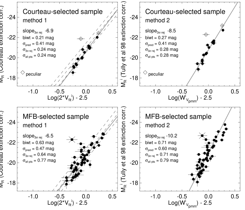
Figure 5: Comparison between TF fits for the NFGS and for the samples of Courteau (1997) and Mathewson et al. (1992, as analyzed by Courteau 1997). The upper panels show NFGS data meeting Courteau’s selection criteria (interpreted to include Sab and Scd galaxies to improve statistics), while the lower panels show NFGS data meeting MFB’s selection criteria (§5.2). Diamonds indicate peculiar/interacting galaxies eliminated from the Courteau-selected sample following Courteau (our peculiarity classification is discussed in §6.2). X’s indicate a galaxy rejected from the MFB sample fits as a $>$3$\sigma$ outlier (but still included in calculating the biweight scatter and $\sigma_{\rm all\,pts}$). Left Panels: NFGS comparison samples analyzed using the methods of Courteau (forward fits, luminosity-independent extinction corrections, $V_{fit}$ velocity parameter, and q${}_{0}=0.18$). Printed parameters and thick gray lines give fit results for the NFGS data. Dashed lines show Courteau’s forward fits to the Courteau and MFB data sets and the $\pm 1\sigma$ scatter on these fits; both fits have been adjusted to H${}_{0}=75$. The Courteau fits have also been shifted from Gunn r to Cousins R using r $-$ R = 0.354 (Jorgensen, 1994), and the MFB fits have been shifted from Cousins I to Cousins R using R $-$ I = 0.5 (Frei & Gunn, 1994, their I_c and R_c). Right Panels: The same data analyzed using our standard techniques (unweighted inverse fits, luminosity-dependent extinction corrections, W${}_{V_{pmm}}$ velocity parameter, and q${}_{0}=0.20$). Printed parameters and thick gray lines give fit results for the NFGS data.

The right panels of Figure 5 demonstrate the effect of switching to our standard analysis techniques. We use unweighted inverse fits (minimizing residuals in velocity width), the W${}_{V_{pmm}}$ velocity parameter, and luminosity-dependent extinction corrections (Tully et al., 1998). With these conventions, the slope of the TFR steepens considerably, and the measured scatter about the fit increases, despite the smaller scatter perceived by eye. The eye perceives the scatter in velocity width, whereas we measure the scatter in absolute magnitudes: the scatter in absolute magnitudes increases as a result of the steeper slope of the TFR. This steeper slope is due in roughly equal measure to the use of inverse fits and to the use of luminosity-dependent extinction corrections.

Another factor affecting scatter is measurement errors. In fact, the good agreement between our scatter and the scatter in the MFB sample should really be taken as evidence that the measurement errors in the two data sets are very similar. For the NFGS subsample defined by MFB’s criteria and analyzed using our standard techniques (lower right panel of Figure 5), we calculate that 0.60 mag of the observed 0.71 mag of scatter arises from measurement errors, leaving only $\sim$0.38 mag of intrinsic scatter after subtraction in quadrature. The NFGS subsample error budget includes four contributions added in quadrature: photometry errors and Hubble-law distance uncertainties (0.18 mag, dominated by the contribution of the peculiar velocity field); photometric inclination errors (0.42 mag, dominated by the one-decimal place precision of the UGC axial ratios); velocity width uncertainties (0.38 mag, dominated by intrinsic scatter in the correspondence between “true” rotation velocities and measured optical velocity widths, regardless of high-quality rotation curves); and extinction correction errors (0.09 mag, derived from the uncertainties in inclination and velocity width). For the MFB sample, inclination errors should be somewhat smaller. MFB galaxies are generally larger on the sky than NFGS galaxies, so assuming that the photometric inclinations for the MFB sample were computed using axial ratios with round-off precision at least comparable to that of the UGC (and with at least comparable accuracy), the MFB inclinations will almost certainly be better than ours. If we ascribe the (slight) scatter difference between the MFB and NFGS samples entirely to the difference in inclination errors, then we infer MFB inclination errors of $\sim$0.3 mag.

5.3 Comparison with Cluster Samples

Except for its restriction to a single environment, the Ursa Major sample of Verheijen & Sancisi (2001, hereafter VS) is almost as broadly representative as the NFGS. Like the NFGS, the VS sample is morphology-blind, including both Sa galaxies and peculiar and interacting galaxies. Here we restrict both samples to M${}_{\rm R}^{i}<-18$, type Sa–Sd, and $i>45$. Within these limits VS’s H I data set is nearly complete, with only one Sa galaxy missing.

Figure 6 directly compares the NFGS and VS spiral samples. With distance scales, extinction corrections, and velocity width definitions matched as described in the figure caption, we detect no zero point offset within the errors. The slope of the VS sample appears considerably shallower, but inspection of the data reveals that the behavior of a few galaxies at the faint end of the TFR accounts entirely for the difference. In §8.4 we discuss possible reasons for the divergence of the two samples at the faint end.

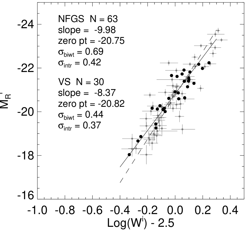
Figure 6: Comparison of TFRs for the NFGS (gray) and for the Ursa Major sample of Verheijen & Sancisi (2001, black), with both samples restricted to types Sa–Sd, M${}_{\rm R}<-18$, and $i>45$. Solid and dashed lines are unweighted inverse fits to the VS and NFGS data respectively. Biweight scatter values are with respect to the corresponding fits. Intrinsic scatter values are computed by subtracting measurement-error scatter in quadrature (see §5.3). We have recomputed VS’s extinction corrections using the original $W_{R}^{i}$ definition of Tully & Fouque (1985) to exactly reproduce the method used for the NFGS corrections (§4.2). $W^{i}$ is W${}_{V_{pmm}}^{i}$ for the NFGS (§3.3) and W${}_{50}^{i}$ for the VS sample; these linewidth measures are calibrated to the same scale in Appendix B. To match VS’s distance scale (18.6 Mpc to Ursa Major), we temporarily adopt H${}_{0}=77$ for NFGS galaxy distances; this value of H₀ and the corresponding Ursa Major distance were both derived from the same Cepheid-based distance calibration (Tully & Pierce, 2000). Note that we find an Ursa Major distance of 16.9 Mpc, which would shift the cluster TFR $\sim$0.2 mag fainter, if we simply apply the Tully & Pierce value of H₀ to the group velocity of Ursa Major ($V\sim 1000$ km sec${-1}$ with respect to the Local Group) and correct for Virgocentric infall at the coordinate center of Ursa Major according to the same prescription used for NFGS recession velocities.

The sources of measurement error for the Ursa Major sample are qualitatively different than for the NFGS, so we must compare intrinsic scatter values, formed by subtracting measurement-error scatter from observed scatter in quadrature. We predict the measurement-error scatter for VS using the same code with which we propagate our own errors, which yields a total predicted R-band scatter of 0.24 mag from four sources: hybrid kinematic-photometric inclination errors (0.09 mag); H I linewidth errors (0.13 mag); distance uncertainties from cluster depth effects (0.17 mag, as estimated by Verheijen, 2001); and errors in photometry and extinction corrections (0.06 mag). These numbers are based on the inclination and H I linewidth errors given by VS combined with basic photometry errors of $\sim$0.05 mag (Verheijen, 2001). Because the NFGS error budget is dominated by inclination errors, it is worth mentioning that VS’s inclination errors are smaller than ours not so much because they sometimes use kinematic inclinations, as because their photometric inclinations are better than ours. Our inclination errors would probably be comparable to theirs if our galaxies were equally large on the sky: the one-decimal-place precision of the UGC adds greater round-off error for galaxies of smaller angular diameter. To illustrate this, we have recomputed photometric inclinations for the Ursa Major sample using UGC axial ratios and the method of §3.4. Substituting these inclinations for VS’s preferred inclinations only slightly increases TF scatter.

After subtracting measurement-error scatter in quadrature, we obtain very similar intrinsic R-band scatter values for the NFGS and the Ursa Major sample: 0.42 mag and 0.37 mag. Similar agreement is found in the B band. Recomputing the NFGS scatter and errors about the shallower slope of the Ursa Major sample, we find even better agreement, but if the NFGS velocity width errors are slightly overestimated (§5.1) then the intrinsic NFGS scatter about the Ursa Major slope may still be as high as $\sim$0.42 mag. The moderately higher intrinsic scatter of the NFGS compared to Ursa Major should not be at all surprising, as the NFGS includes a wide range of environments and star formation histories. Apart from the hint of a systematic offset at the faint end mentioned previously, the two samples are in excellent agreement.

Other cluster TF studies quote lower scatter than we find for the complete Ursa Major sample.

For example, combining data from multiple clusters (including Ursa Major, Fornax, Coma, the Pisces Filament, and several others), Tully & Pierce (2000) measure an R-band scatter of 0.34 mag. Sakai et al. (2000) obtain the same result with a partially overlapping data set and similar analysis techniques. However, directly comparing the NFGS spiral sample with these multi-cluster samples would be misleading, for several reasons. First, each individual cluster in the multi-cluster samples obeys a different definition of “complete” and satisfies that definition to a different degree. For example, the “complete” Fornax sample rejects interacting or disturbed galaxies and multiple systems (Bureau et al., 1996). Second, each cluster represents a different environment with a different star formation history, so each cluster’s color–magnitude relation may have a different color zero point (e.g. Tully & Pierce find $B-I$ color zero point offsets of $\sim$0.1 mag when they compare cluster color–magnitude relations; see also Watanabe et al., 2001). We will see in §7.2.1 that if real, such color offsets almost certainly imply TF zero point offsets between the clusters. However, the TF scatter due to these TF zero point offsets is suppressed in the multi-cluster analyses to the extent that the individual cluster TFRs are allowed to shift freely to minimize zero point offsets (the absolute zero point is generally determined separately using the Cepheid calibrator galaxies). A third concern is the effect of a top-heavy luminosity distribution: in combining more distant clusters with more nearby ones, the multi-cluster studies define samples that statistically favor bright galaxies. This bias may drive down scatter if fainter galaxies have higher scatter. While the existence of such a trend is unclear in our restricted spiral sample, dwarf galaxies definitely show higher scatter in the full sample (§8).

6 The Spiral TFR 2: Sa & Peculiar Galaxies

We have shown that our TF results are consistent with previous studies if we reproduce their sample selection criteria. These criteria often exclude Sa galaxies and/or galaxies with morphological peculiarities. Here, we begin the process of analyzing TF scatter for a broad spiral sample by turning the spotlight on Sa and peculiar galaxies, highlighting where these galaxies’ TF residuals fall within the general spiral TFR. For this analysis we return to the full NFGS spiral TF sample: types Sa–Sd brighter than M${}_{\rm R}^{i}=-18$ and inclined by $>$40$\arcdeg$.

6.1 An Sa Galaxy Offset

Fourteen of the 68 galaxies in the NFGS spiral TF sample are Sa–Sab galaxies, collectively referred to as “Sa” galaxies from here on. As a group, these 14 galaxies sit clearly to one side of the TFR (Figure 7), with offsets toward lower $L$/higher $W^{i}$ of 0.76 mag at R, 0.95 mag at B, and 1.20 mag at U as compared to Sb–Sd galaxies (where both Sa and Sb–Sd offsets are computed with respect to the unweighted inverse TF fits in Table 1, with relative offset uncertainties of $\sim$0.17 mag).

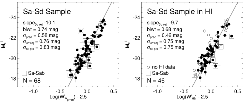
Figure 7: TFR for the Sa–Sd sample, illustrating the Sa galaxy offset toward higher $W^{i}$/lower $L$. The left panel uses optical velocity widths while the right panel uses H I linewidths, with missing data points indicated by an open circle at the position of the optical velocity width. Lines show unweighted inverse fits to the solid points.

The possibility that Sa galaxies rotate faster at a given luminosity was first suggested by Roberts (1978) based on 21 cm data. Sa offsets became controversial after Rubin et al. (1985) claimed that the Sa TFR lies 2 mag below the Sc TFR in the B band. Other studies reported smaller offsets (e.g. Pierce & Tully, 1988). Simard & Pritchet (1998) argue that a greater intrinsic spread of luminosities for late-type vs. early-type galaxies at a given velocity width, combined with Malmquist bias, may explain the large offset found by Rubin et al. (1985). However, Sa offsets continue to be observed in increasingly complete samples (e.g. Verheijen, 1997, see §7.2.1).

The scatter properties of our data suggest that the offset we observe is mostly real. In the R band, the Sa galaxies and the Sb–Sd galaxies have biweight TF scatter values of 0.63 mag and 0.70 mag, respectively. These numbers imply that Malmquist bias is unlikely to produce the observed 0.76 mag offset between the two populations. In the B and U bands, the scatter in each population increases but the offset increases even more. The offset exceeds the scatter by 0.3 mag at U.

We have investigated whether the Sa offset in our data may be ascribed to systematic errors in luminosity or velocity width measurements. For example, large bulges could make Sa galaxies appear rounder (and more face on) than they really are, leading to underestimated extinction corrections and overestimated $\sin i$ corrections. Sa’s in the present sample do have more face-on inclination estimates on average (61$\arcdeg$ vs. 66$\arcdeg$ for the full spiral TF sample); however, this difference can account for an offset of only $\sim$0.2 mag at a TF slope of $-$10. Furthermore, even extreme assumptions about axial ratios (e.g. assigning an intrinsic axial ratio of $q_{0}=0.4$ to Sa’s and assigning $q_{0}=0.09$ to all other types) reduce the R-band offset by at most half and have much less effect in the B and U bands. No other aspect of our analysis is responsible for the offset either. Whether we adopt luminosity-dependent or independent extinction corrections has negligible effect on our results. We do not add an explicit morphological type dependence to our extinction corrections, but in any case adding such a dependence would probably only increase the Sa offset: extinction is likely to be lower in Sa galaxies (Kodaira & Watanabe, 1988). The offset is not appreciably affected when we substitute $V_{fit}$ for $V_{pmm}$ or when we omit the optical-to-radio conversion. Finally, the available H I data also seem to confirm the offset (Figure 7), although these data are subject to incompleteness and high scatter for the Sa population.

We conclude that the bulk of the Sa offset in our sample is real. However, with just 14 Sa galaxies, our analysis is subject to small number statistics. Formally, a Kolmogorov-Smirnov test yields a probability of $6\times 10^{-4}$ that the R-band TF residuals of the Sa and Sb–Sd subpopulations were drawn from the same parent population ($\sim$3.5$\sigma$). A possible physical explanation for the Sa offset and a way to remove the offset to reduce scatter will be discussed in §7.2.1.

6.2 Galaxy Peculiarity and Sample Pruning

TF samples are frequently pruned to remove morphologically peculiar galaxies and sometimes also to remove barred galaxies. Here we use the term “peculiar galaxies” to mean disturbed spiral galaxies (i.e. those with warps, tidal features, multiple nuclei, polar rings, or interacting neighbors) rather than galaxies that cannot be reliably classified as spirals. Figure 8 shows rotation curves and images for three NFGS galaxies we have identified as morphologically peculiar. To avoid bias, bars and morphological peculiarities were independently identified by two of us (S.K. and M.F.) without reference to TF residuals, and the identifications were further checked against the notes provided by R.A. Jansen in Jansen et al. (2000b). Although a number of weak bars and peculiarities were noted, we report here only strong, unambiguous cases identified by more than one observer. Such cases are broadly distributed across a wide range of spiral types and luminosities.

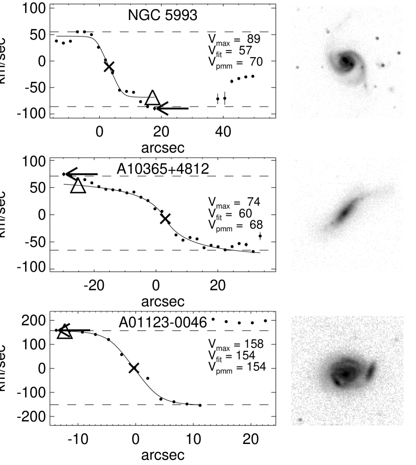
Figure 8: B-band images and rotation curves for three galaxies with morphological peculiarities (§6.2). Notation is as in Figure 4. The distinct kinematic components at large radii in the first and third panels were not used in computing velocity widths. Images are courtesy of Jansen et al. (2000b).

Figure 9a uses two different (possibly overlapping) symbols to identify peculiar and barred galaxies within the NFGS TFR. Although the barred galaxies that are not peculiar do not show a clear systematic offset, the peculiar galaxies as a group tend to lie on the high $L$/low $W^{i}$ side of the TFR. This pattern suggests that pruning such galaxies may obscure interesting physics hidden in TF scatter.

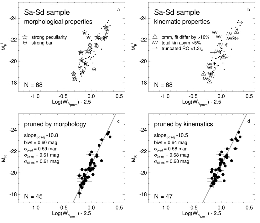
Figure 9: Upper Panels: Location of kinematically and morphologically peculiar galaxies within the Sa–Sd TFR. Lower Panels: Effect of pruning the sample to remove such galaxies. Unweighted inverse fit results are shown.

Even when the goal is scatter reduction, pruning may not be the most effective strategy. Figure 9c demonstrates that pruning barred and peculiar galaxies from the NFGS spiral sample reduces R-band TF scatter to approximately the level expected from measurement errors. In bluer passbands, however, the reduced scatter still exceeds the level expected from measurement errors: we measure 0.63 mag and 0.71 mag in B and U, respectively, compared to a predicted measurement-error scatter of 0.58 mag in both passbands. Also, the decrease in scatter won by pruning comes at a high price, as $>$30% of the sample must be rejected. In §7 we will use more objective, physically motivated techniques to reduce TF scatter to a level comparable to measurement-error scatter in all passbands without discarding galaxies from the sample.

We have also considered independent definitions of peculiarity involving kinematic data: Figure 9b identifies galaxies with truncated rotation curves ($r_{max}<1.3r_{e}$, §3.3), rotation curve asymmetries greater than 5% (our RC asymmetry index is defined in Appendix C), or discrepancies between W${}_{V_{fit}}$ and W${}_{V_{pmm}}$ greater than 10%. Interestingly, galaxies with high RC asymmetry behave much like those with strong morphological peculiarities, with high $L$/low $W^{i}$ offsets. Figures 9c and 9d show that pruning based on either morphology or kinematics produces a comparable reduction in scatter, although kinematic pruning misses some Sa outliers.

To test whether our definitions of kinematic peculiarity have physical significance or merely identify faulty rotation curves, we have tried pruning the H I linewidth TFR using kinematic peculiarity information obtained from our optical RCs. Amazingly, optical RC peculiarities are at least as effective as morphological peculiarities in flagging outliers in the H I linewidth TFR. This result implies that either (1) optical RC peculiarities are associated with observational errors in the NFGS surface photometry or the UGC-derived photometric inclinations common to both the H I and optical RC TFRs, or (2) optical RC peculiarities occur in galaxies that lie off the TFR for physical reasons. We find evidence for the latter in §7.

7 The Spiral TFR 3: Third Parameters & Physical Sources of Scatter

We have seen that interacting, merging, and peculiar galaxies often lie on the high $L$/low $W^{i}$ side of the TFR, while Sa galaxies lie on the low $L$/high $W^{i}$ side (§6). Figure 10 shows that in addition, NFGS galaxies brighter than M${}_{\rm R}^{i}\sim-22.5$ display asymmetric scatter about the best-fit TFR for fainter galaxies, with a systematic offset of $\sim$0.7 mag toward lower $L$/higher $W^{i}$. Below we demonstrate that all of these offsets reflect underlying correlations between TF residuals and quantitative galaxy properties, most notably $B-R$ color and H$\alpha$ equivalent width (EW). Following tradition, we refer to these properties as “third parameters,” i.e. additional variables that control physical scatter in the two-parameter TFR.

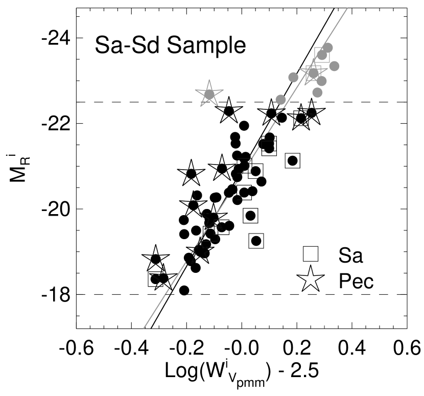
Figure 10: Systematic offsets in the Sa–Sd TFR. Sa and peculiar galaxies fall on opposite sides of the TFR, helping to drive strong correlations between TF residuals and physical properties such as effective $B-R$ color and global EW(H$\alpha$). In §7 we quantify the statistical significance of these correlations within the luminosity range between the dashed lines. This range excludes the asymmetric scatter at the bright end of the relation to ensure fair statistical tests (§7.1). The gray and black lines show unweighted inverse TF fits to the sample with and without galaxies brighter than M${}_{\rm R}^{i}=-22.5$. For statistical tests, we define residuals relative to the black line.

7.1 Third Parameter Analysis Technique

Barton et al. (2001) demonstrate that false correlations between TF residuals and candidate third parameters may arise when the TF slope is measured incorrectly, in which case any parameter that varies along rather than perpendicularly to the TFR will produce a correlation. A true third parameter should vary at least partly perpendicularly to the TFR.

We adopt the following strategy to avoid false detections of third parameters. First, we apply strict cuts in Mⁱ to eliminate sections of the data where the velocity width scatter is clearly asymmetric. For the R band, these cuts are indicated by the dashed lines in Figure 10 (see also Table 2): the upper line excludes galaxies brighter than M${}_{\rm R}^{i}\sim-22.5$, which show a systematic offset as discussed above, and the lower line excludes galaxies that do not meet the M${}_{\rm R}^{i}<-18$ sample definition criterion. After these cuts, the data are biased in Mⁱ but nearly perfectly unbiased in velocity width. Second, we apply an inverse TF fit to the data, which minimizes residuals in velocity width. At this point the velocity width residuals are completely uncorrelated with luminosity Mⁱ. Finally, we use Spearman rank tests to quantify both the candidate third parameter–TF residual correlation and the candidate third parameter–luminosity correlation. For the Spearman tests, velocity width residuals and magnitude residuals are interchangeable. If these tests show that the candidate third parameter correlates with TF residuals but not with luminosity, then we conclude that it varies perpendicularly to the TFR.

Table 2: Magnitude Cuts for Spearman Rank Tests 

	U	B	R
bright cut	-21	-21	-22.5
standard faint cut	-17	-17	-18
dwarf faint cut	-16	-16	-17

In fact, even if a parameter does vary with luminosity, it may still qualify as a third parameter if it also correlates clearly with TF residuals, because we have in principle eliminated the TF residual–luminosity correlation. Nonetheless, one must be wary if the parameter-luminosity correlation is stronger than the parameter–TF residual correlation, as in such a case even small TF slope errors may lead to false correlations. For luminosity-dependent parameters, one may wish to subtract out the luminosity dependence and measure the correlation between TF residuals and “parameter residuals,” i.e. parameter offsets from the fitted parameter–luminosity correlation (cf. Courteau & Rix, 1999). Below we give results based on raw parameters, but we have also checked our results using parameter residuals. The parameter–luminosity correlations are strongest for color and rotation curve asymmetry (Figure 11); however, even for these parameters we find that correcting for the luminosity dependence makes little difference, slightly improving the third-parameter correlation if anything.

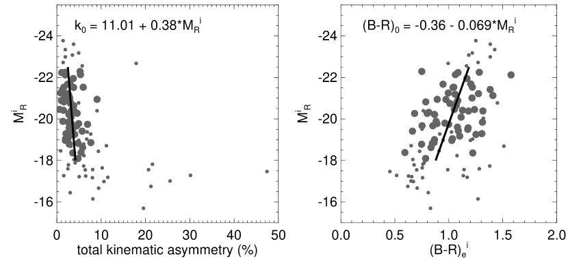
Figure 11: M${}_{\rm R}^{i}$ vs. total RC asymmetry (Appendix C) and effective $B-R$ color. Larger points represent the luminosity and inclination-restricted spiral sample of Figure 10, while smaller points show other galaxies in the optical RC sample. Galaxies with $i<40$ are excluded from both panels. Black lines represent least-squares inverse fits to the larger points, minimizing residuals in color and RC asymmetry. Note that inverse fits are appropriate for combining with our inverse TF fits; some bias is clear in the line slopes, but it has no effect on our conclusions.

In general, we use unweighted TF fits to define TF residuals. Unweighted fits avoid the slope bias that would otherwise arise because our errors vary systematically with luminosity and velocity width. However, we have confirmed all correlations using both weighted and unweighted fits. We have also confirmed all correlations using two definitions of velocity width (W${}_{V_{fit}}$ and W${}_{V_{pmm}}$) and using both luminosity-dependent and luminosity-independent extinction corrections (§4.2). Results quoted in the text use W${}_{V_{pmm}}$ and the Tully et al. (1998) extinction corrections.

7.2 Third Parameter Test Results

We have tested a wide range of candidate third parameters, making use of photometric and spectrophotometric quantities from the NFGS database (Jansen et al., 2000a, b) and photometric asymmetries kindly provided by R. Jansen (private communication, see also Jansen, 2000). For the luminosity-restricted Sa–Sd sample of Figure 10, TF residuals correlate strongly with $(B-R)_{e}$ (effective $B-R$ color measured within the B-band half-light radius) and global EW(H$\alpha$) in all bands. Other measures of color and emission-line strength yield somewhat noisier correlations. We also find correlations with rotation curve asymmetry, photometric asymmetry, and two measures of surface brightness; these correlations reach $>$3$\sigma$ significance only in certain photometric bands. TF residuals do not correlate with luminosity (by construction) or with inclination, validating our analysis. Likewise, we detect no correlation between TF residuals and rotation curve extent, isophotal radius, effective radius, H I gas mass, gas consumption timescale, or $M_{\rm HI}/L$ (we have incomplete data for the last three however, see §7.2.6).

Figure 12 displays some of the correlations in the R band and lists Spearman rank test results for U, B, and R (the “probability of no correlation” $p$ is given, where $1-p$ is the confidence of the result). The symbol coding shows that Sa and peculiar galaxies drive most of the statistical signal in the R-band correlations. If we eliminate both groups of galaxies, no R-band correlation survives with $>$3$\sigma$ confidence. However, the $(B-R)_{e}$ correlation does survive in B, and both color and emission line correlations remain significant in U. In general, the two groups of galaxies contribute roughly equally to the correlations, with the Sa galaxies showing a slightly stronger signal due to lower scatter. The peculiar galaxies form a more heterogeneous group, including not only interacting, merging, and warped galaxies, but also a few galaxies whose oddities may indicate later evolutionary states, e.g. a bulge-dominated Sa galaxy with a prominent polar dust lane (NGC 984).

Figure 12: TF residuals vs. physical properties of the Sa–Sd $i>40$ $-18<\rm M^{i}_{\rm R}<-22.5$ sample (see also Figure 10). Squares indicate Sa galaxies and stars indicate galaxies with morphological peculiarities (§6.2). The Spearman rank probability of no correlation between the parameter and TF residuals in each optical band is given as $p_{band}$. Only R-band TF residuals are plotted. Dashed and dotted lines in the top panels show forward least-squares and least-squares bisector fits (Isobe et al., 1990, see §7.3.1). Colors in the top right panel are defined relative to the color–magnitude relation (Figure 11).

Although Sa and peculiar galaxies dominate the statistical signal we measure, the correlations in Figure 12 apply to all galaxies in the sample. A blue, strongly star-forming galaxy whose image does not appear peculiar nonetheless shows the expected TF residual. Thus the correlations provide a physical, quantitative basis for understanding systematic offsets in the TFR, independent of morphological classification.

Furthermore, the correlations are not limited to the optical TFR. Despite disproportionate H I catalog incompleteness for bright and peculiar galaxies, mixed H I data quality, and confusion in single-dish linewidths, we still detect 2–3$\sigma$ correlations between radio TF residuals and both $(B-R)_{e}$ and global EW(H$\alpha$). We also find evidence for a TF residual–total color correlation in radio data from the complete Ursa Major database of Verheijen & Sancisi (2001), see §7.2.1. These results emphasize the close link between optical and radio velocity widths already noted in §3.3 and §6.2 (see also Appendix B). However, we do not perform a detailed third-parameter analysis of the radio TFR, as the catalog H I linewidths are incomplete and of mixed quality.

7.2.1 Color

Effective $B-R$ color yields a striking correlation with TF residuals, predicting spiral galaxy TF offsets better than any other physical parameter we have tested. Effective $U-B$ color also produces a clear correlation in all three bands. The color–TF residual correlations strengthen from R to B to U, as blue peculiar galaxies and red Sa galaxies move further apart in the TFR. Although we correct colors for internal extinction (see §4.2), omitting the extinction correction does not significantly affect the correlation strength. The correlation slope is quite a bit steeper than expected from dust extinction and reddening ($\sim$1.3 in the R band with $B-R$ colors, e.g. Gordon et al., 1997, Table 1).

We stress that the correlation reported here cannot be dismissed as merely the “built-in” correlation due to the variation of TF scatter with passband. A weak correlation of U and B-band TF residuals with color might have been expected from the fact that TF scatter is significantly higher in these bands than in the R band, which implies that both $B-R$ and $U-R$ colors may be used to reduce scatter (most trivially, simply by adding these colors to the U and B magnitudes to recover the R magnitudes). In this case, the color–TF residual correlation would have a slope of $\sim$1 and there would be no correlation between R-band TF residuals and $B-R$ colors. However, both the persistence of the correlation in the R band and the steep slope of the correlation point to a more interesting result: we explore this result empirically in this section and discuss its physical significance in §7.3.

For our sample, effective colors produce much tighter correlations than total colors. In the R band, Spearman tests yield $p=6.1\times 10^{-5}$ for the ($B-R$)${}_{e}^{i}$ correlation, or $\sim$4$\sigma$, but only $p=0.034$ for the total ($B-R$)ⁱ correlation, or just over 2$\sigma$. Total colors dilute the correlation signal with observational scatter from profile extrapolation and background subtraction (R. Jansen, private communication). However, we see no strong systematic differences between $B-R$ and $(B-R)_{e}$: on average the two track closely, with $(B-R)_{e}$ slightly redder, by at most $\sim$0.1 mag for the reddest galaxies.

The color–TF residual correlation offers an alternative to sample pruning for reducing TF scatter. If we restore spiral galaxies brighter than M${}_{\rm R}^{i}=-22.5$ to the sample (they were not used in Figure 12, see Figure 10), then refitting the color–TF residual correlation provides a color-correction formula to go with the unweighted inverse TF fit in Table 1. A least-squares forward fit to $\Delta$M vs. $(B-R)_{e}^{i}$ yields

$$\Delta\rm M_{\rm R}^{i}=-2.0+1.8(B-R)_{e}^{i}$$ (5)

where $\Delta\rm M_{\rm R}^{i}$ is the measured TF residual (observed magnitude minus fitted relation). If we correct our R-band magnitudes with equation 5 and recompute the residuals with respect to the original TF fit, the biweight scatter falls from 0.74 mag to 0.66 mag. An analogous procedure reduces scatter to 0.64 mag in both the B and U bands, from 0.82 and 1.02 mag respectively, essentially eliminating the differences between wavelength bands (Figure 13). The corrected scatter values come quite close to the scatter expected from measurement errors (Table 1). Determining whether these errors hide further non-random behavior in TF scatter would require smaller measurement errors. Full two-dimensional velocity fields, with kinematic inclinations and modeling of disk warps and asymmetries, offer the best hope of progress (cf. Bershady & Andersen, 2000).

Figure 13: Scatter reduction in the U-band TFR using a fit to the effective color–TF residual correlation (§7.2.1). Diamonds show the original points and dots show the color-corrected points. Note that the corrected points define a steeper slope due to the color-magnitude relation. The biweight scatter for the original and color-corrected magnitudes is given in mag.

The existence of a strong color–TF residual correlation is not entirely unexpected. Pierce & Tully (1992) describe environmental shifts in the B-band TFR for a mixed cluster-field sample that are linked to galaxy colors, which suggests the possibility of a color–TF residual correlation. Giraud (1986) demonstrates reduced TF scatter in a two-color Tully-Fisher relation (essentially equivalent to our color-corrected TFR, as in Figure 13, but with the slope of the color–TF residual correlation assumed rather than measured). Rhee (1996) reduces TF scatter using 60 $\mu$m data to define “population corrected” luminosities. Bershady et al. (1999) present initial evidence for a color–TF residual correlation in their intermediate-redshift sample, which spans a wide range of galaxy types; however, the TF residuals are measured relative to an externally defined TFR, making it harder to eliminate systematic errors (also a potential problem for Zaritsky (1995), see Barton et al. (2001) and the discussion in §7.1). Most significantly, Verheijen (2001) reports a $B-I$ color vs. TF residual correlation for a subsample of 21 galaxies drawn from his complete Ursa Major sample, and our own analysis of his full Sa–Sd data set indicates that total $B-R$ colors correlate with B-band TF residuals at $\sim$3–3.5$\sigma$ confidence (using unweighted inverse fits, our standard luminosity cuts, and the W₅₀ and M${}_{\rm B}^{i}$ from Verheijen & Sancisi, 2001). The R-band correlation for this sample registers at $\sim$2$\sigma$, consistent with our expectations given that total rather than effective colors were used.

Most other low-redshift TF studies exclude Sa and peculiar galaxies and/or use red to near-infrared photometry, making it difficult to observe the color–TF residual correlation. For example, Courteau & Rix (1999) find only a slight, statistically insignificant color–TF residual correlation in a sample of undisturbed Sb–Sc galaxies observed in the R band. The close galaxy pairs sample of Barton et al. (2001) includes disturbed galaxies but was not designed to evenly sample the range of spiral morphologies; again no correlation emerges using total colors and R-band TF residuals (E. Barton, private communication).

The color–TF residual correlation provides a natural explanation for two effects noted previously: the Sa galaxy offset (§6.1) and the asymmetric scatter at the bright end of the TFR (§7). Sa galaxies are typically red and show relatively little scatter in color compared to later type galaxies (Jansen et al., 2000b). As a consequence, Sa galaxies deviate from the TFR as a group, with larger offsets in bluer bands. Applying the color correction given in Equation 5 reduces the R-band offset between Sa and Sb–Sd galaxies from 0.76$\pm$0.17 to 0.28$\pm 0.23$ mag, where we have computed offsets using TF residuals relative to the unweighted inverse fit in Table 1. The remaining offset is not statistically significant. Similarly, the $\sim$0.7 mag offset for galaxies brighter than M${}_{\rm R}^{i}=-22.5$ shrinks to $\sim$0.15 mag following the color correction, suggesting that the asymmetric scatter at the bright end of the TFR may simply reflect the rarity of extremely luminous blue galaxies.

Verheijen (2001) has also reported a link between color dependence and morphological type dependence in the TF residuals for his pruned Ursa Major spiral sample. The Sa and Sab galaxies are underluminous by $\sim$0.5 mag in the B band (consistent with our result when normalized for slope differences, $-$6.7 vs. $-$10), while the same galaxies have normal luminosities at K, suggesting a color effect. Later types show a wide range of positive and negative TF residuals in both Verheijen’s complete TF sample (Verheijen, 1997) and in the NFGS spiral TF sample, consistent with the much greater color dispersion observed for types Sb and later in the full NFGS (Jansen et al., 2000b). We discuss a physical interpretation of the color–TF residual correlation in terms of stellar populations in §7.3.

7.2.2 Emission Line Strength

Global H$\alpha$ equivalent width (integrated over the entire galaxy, see Jansen et al., 2000a) correlates with TF residuals for the Sa–Sd subsample almost as well as $(B-R)_{e}$ (Figure 12). This result should not be too surprising: the two parameters are highly correlated. EW(H$\alpha$) measures recent star formation on timescales of Myr relative to integrated past star formation, while $(B-R)_{e}$ measures the ratio between young and old stellar populations and thus traces star formation on timescales of Gyr (e.g. Kennicutt et al., 1994). As expected, the EW(H$\alpha$)–TF residual correlation intensifies in bluer TF bands, although not quite so strongly as the color correlation. Substituting either nuclear (fixed $3^{\prime\prime}\times 7^{\prime\prime}$ aperture) H$\alpha$ or global [OII] 3727 measurements for global H$\alpha$ weakens the correlation, but it still reaches $>$3$\sigma$ significance in the B and U bands.

Restoring spiral galaxies brighter than M${}_{\rm R}^{i}=-22.5$ to the sample, we can fit an EW(H$\alpha$)-correction formula analogous to the color-correction formula in equation 5:

$$\Delta\rm M_{\rm R}^{i}=0.5+0.026EW(H\alpha).$$ (6)

For the unweighted inverse fits in Table 1, this formula and its B and U analogues reduce scatter to 0.66, 0.67, and 0.78 mag in the R, B, and U bands respectively. The EW(H$\alpha$) correction thus performs nearly as well as the color correction in both B and R, although it underperforms in U.

To our knowledge, this paper is the first to report a correlation between TF residuals and EW(H$\alpha$). Barton et al. (2001) search unsuccessfully for such a correlation using nuclear (fixed slit) H$\alpha$ measurements and R-band TF residuals. These results are consistent, given that (a) our sample yields only a 2.9$\sigma$ correlation between R-band TF residuals and nuclear EW(H$\alpha$), and (b) the Barton et al. survey targets a specific population (galaxies in close pairs) rather than a broad cross-section of galaxies.

7.2.3 Photometric Asymmetry

The existence of a correlation between TF residuals and photometric asymmetry has not been firmly established. Zaritsky & Rix (1997) argue that I-band asymmetry and B-band TF residuals are correlated, but Barton et al. (2001) suggest that the bulk of this correlation arises from a systematic error in TF calibration. We measure no significant correlation of R-band asymmetry with TF residuals in any passband, but we do see a marginal 3$\sigma$ correlation between B-band asymmetry and R-band TF residuals, which weakens for B and U-band residuals. We conclude that photometric asymmetry is a weak third parameter at best. Since asymmetry arises from multiple causes that may move TF residuals in different directions (knottiness from dust, unevenness from recent starbursts or accretion, etc.), sample selection may partly determine whether or not a correlation is detected.

7.2.4 Rotation Curve Asymmetry

Rotation curve asymmetry (defined in Appendix C) correlates with TF residuals in the B and U bands with $\sim$3$\sigma$ significance. The RC asymmetry vs. TF residual plot (Figure 12) may also indicate a discrete effect: galaxies with asymmetry less than $\sim$2% show lower scatter and a slight offset relative to those with higher asymmetry. Barton et al. (2001) also report a discrete effect in their close pairs sample: the R-band TF residuals of galaxies identified as severely kinematically distorted differ from the residuals for the remaining galaxies by 3$\sigma$ in a K-S test. We return to the possible link between kinematic distortions and TF offsets in §7.3.2.

7.2.5 Surface Brightness

Courteau & Rix (1999) argue against any surface brightness dependence in the TF residuals of high surface brightness spiral galaxies, while O’Neil et al. (2000) demonstrate that extreme low surface brightness (LSB) galaxies can lie well off the TFR. In our sample we find no clear correlation in any passband with the most common measure of surface brightness used in the literature, the extrapolated disk central surface brightness (as measured from exponential profile fits, R. Jansen, private communication). On the other hand, we do detect marginal correlations between TF residuals and two other measures of surface brightness. The observed R-band central surface brightness (measured from raw profiles including both disk and bulge light, and subject to uncertainties due to both seeing and the distance to the galaxy) correlates with U and B-band TF residuals at $>$3$\sigma$, but the detection has high uncertainty due to a strong central surface brightness–luminosity correlation (which causes the third parameter correlation to weaken if weighted TF fits are used, see §7.1), and it disappears for the full sample. A more robust quantity, the effective surface brightness in the U band ($\mu_{e}^{U}$, the surface brightness measured at $r_{e}$) displays a 3$\sigma$ correlation with R-band TF residuals, but this correlation fades in the B and U bands (Figure 12). However, the correlation becomes stronger for the full sample; we discuss it in §8.2.2.

7.2.6 Neutral Gas Properties

The present spiral sample shows no correlation between TF residuals and neutral gas properties such as $M_{\rm HI}$, gas consumption timescale, and $M_{\rm HI}/L$, where we determine $L$ in the same passband as the TF residuals to eliminate any correlation due to color. However, we compute gas masses from the catalogs of Bottinelli et al. (1990) and Theureau et al. (1998), and these catalogs do not provide H I masses for $\sim$31% of the Sa–Sd subsample. The incompleteness preferentially affects Sa and peculiar galaxies, which have the largest TF offsets, so our results should be treated with caution.

Nonetheless, our failure to detect an $M_{\rm HI}$–TF residual correlation is interesting in light of the strength of the $M_{\rm HI}$–luminosity correlation. For the Sa–Sd subsample, the $M_{\rm HI}$–luminosity correlation rivals the TFR itself in correlation strength: although weaker at B and R, it is actually stronger at U, with a Spearman rank probability of no correlation of $10^{-11}$. Therefore even a small TF slope error could easily generate a false correlation between TF residuals and H I mass in this sample. The fact that we detect nothing validates our fitting and analysis procedures, as H I masses and TF velocity widths are measured completely independently. Furthermore, since the color–luminosity correlation is much weaker than the H I mass–luminosity correlation in our data, this argument supports our claim that slope errors do not drive the strong correlation we observe between color and TF residuals.

7.3 What Causes Offsets from the Spiral TFR?

The existence of a well-defined Tully-Fisher relation for spiral galaxies suggests that for large disk galaxies, the total mass of the system (traced by its rotation velocity) closely couples to the mass of its stars (traced by their luminosity). TF residuals may arise from any of three basic relations underlying the overall relation: (1) the relation between observed rotation velocity and total mass, (2) the relation between total mass and stellar mass, and (3) the relation between stellar mass and observed luminosity. Below, we examine the possibility that variations in stellar $M/L$ due to differences in stellar populations can fully explain the color–TF residual correlation, with TF offsets interpreted as luminosity offsets. We then discuss alternative explanations for the color–TF residual correlation that interpret TF offsets as velocity width offsets that correlate with color.

7.3.1 Luminosity Offsets

Variations in stellar $M/L$ due to differences in stellar populations provide the simplest explanation of TF scatter (e.g., Rhee, 1996). Scatter driven by population differences should be higher in bluer passbands, where variations in $M/L$ are greater, and indeed TF scatter increases from R to B to U. If there is negligible scatter in the correlation between rotation velocity and stellar mass (i.e., the combination of relations (1) and (2) above), then the color–TF residual correlation follows directly from the dependence of color on $M/L$, provided that color variations are not dominated by the systematic correlation between color and magnitude (in agreement with our observations, see §7.2.1 and Figure 11). The only caveat is that different star formation histories may yield different ratios of luminosity evolution to color evolution ($LE/CE$), producing different TF offsets for a given color change. Thus we can test the hypothesis that stellar population differences drive the color–TF residual correlation by comparing the slope of the correlation to the $LE/CE$ predictions of population synthesis models designed to describe the general population of spiral galaxies.

We perform this comparison using the model predictions of Bell & de Jong (2001). These authors use population synthesis models to evaluate the slope of the color vs. stellar $M/L$ correlation for passively evolving disk galaxies subject to a variety of star formation histories in which stars form in a reasonably smooth fashion with no major bursts. These slope predictions may be compared to the measured slopes shown in the top two panels of Figure 12. The top right panel shows the color residual–TF residual correlation, where color residuals are defined relative to the color–magnitude relation; this relation offers the most direct measurement of $LE/CE$, suitable for comparison with a simple model such as a closed box model. (One might prefer to define color residuals relative to the color-velocity width relation; however, because our sample is defined by strict limits in magnitude rather than in velocity width, the color-velocity width relation would be biased.) The standard color–TF residual correlation, uncorrected for the color–magnitude relation, may correspond better with models employing mass-dependent star formation histories.

Depending on the particular star formation history used, Bell & de Jong’s predicted slope varies from 1.8–2.5 for R-band TF residuals and $B-R$ colors, with a closed box model giving a slope of 2.3. For the observed correlation, a forward least-squares fit yields a slope of 2.2(2.5) $\pm 0.5$ for the uncorrected(corrected) correlation, while a least-squares bisector fit yields 3.5(3.9) $\pm 0.5$ (cf. Isobe et al., 1990). The latter fit technique is more realistic as it assumes intrinsic scatter in both fit variables; slopes measured by this technique are broadly consistent with the Bell & de Jong predictions but appear to favor slightly steeper values. Slopes measured in the B band are also somewhat steep: e.g. while the closed box model gives a slope of 3.3 in B, we derive values of 3.2 and 4.4 using forward and least-squares bisector fits, respectively, for the color residual–TF residual correlation.

The basic agreement between Bell & de Jong’s predictions and our observations supports our interpretation of the data in terms of stellar populations. With this interpretation we find a single passband-independent stellar-mass TFR (i.e., our “color-corrected” TFR, §7.2.1) with lower scatter than the conventional TFR and a form very similar to that predicted by Bell & de Jong: $L\propto V^{4.6\pm 0.3}$. To the extent that there is any discrepancy between observed and predicted $LE/CE$ ratios, the data would appear to support slightly steeper slopes than the models. This result is largely insensitive to the choice of extinction corrections, even when we omit such corrections altogether, although it is possible to push the observations closer to the models with selected analysis techniques (e.g. adopting the type-dependent $q_{0}$ described in §6.1 and using colors uncorrected for the color–magnitude relation). If real, the steeper slopes might reflect several effects: (1) variations in dark matter fraction or dark matter structure that correlate with color; (2) systematic velocity width offsets due to inclination errors or rotation curve distortions that correlate with color; or (3) star formation histories that include recent starburst activity ($\lesssim$1 Gyr ago), which would give $LE/CE$ ratios $\gtrsim$5 (e.g., Bell & de Jong Figure 5). In support of option (3), many NFGS galaxies show morphological and kinematic evidence of disturbance (§6.2), suggesting the likelihood of starbursts driven by interactions, mergers, or global instabilities. We discuss options (1) and (2) in the next section.

We have also analyzed the color–TF residual correlation for one other complete TF sample, the Ursa Major sample of Verheijen & Sancisi (2001), and we find much shallower slopes ($\sim$1 in R, $\sim$2 in B). These slopes are even shallower than expected purely from population synthesis. As the Ursa Major cluster represents a uniform moderate-density environment, the difference may be related to a greater homogeneity of star formation histories compared to what we see in the general field. In this case the TF residuals in the color–TF residual correlation might have less to do with luminosity offsets related to stellar populations and more to do with color-dependent velocity width offsets driven by one of the mechanisms described in §7.3.2 below.

7.3.2 Velocity Width Offsets

TF residuals are very sensitive to small offsets in velocity width because of the steep slope of the TFR. Therefore any systematic velocity width trends in our data must correlate tightly with color, given the success of the color correction in reducing scatter to near measurement-error levels in all bands (§7.2.1). Possible sources of velocity width residuals include variations in dark matter fraction or dark matter structure, systematic errors in photometric inclination, and symmetric or asymmetric distortions in rotation curves. If any of these correlates strongly with color, it may offer an alternative explanation for the color–TF residual correlation in terms of velocity width offsets rather than luminosity offsets.

A full consideration of dark matter structure is beyond the scope of this paper, but we can address one plausible scenario with straightforward observable consequences. Halo contraction in bulge-dominated galaxies could lead to increased rotation velocities within the central parts of the galaxies, in turn driving a correlation between color and velocity width residuals insofar as higher bulge-to-disk ratios correlate with redder colors. However, the high color dispersion for later morphological types (Jansen et al., 2000b) suggests a relatively weak link between colors and bulge-to-disk ratios, except for early types such as Sa galaxies. Furthermore, the observed RCs for our Sa galaxies do not decrease in velocity in their outer parts, so we have no independent evidence that these galaxies’ high central concentrations have in fact increased their measured rotation velocities. Extended H I data might reveal such an effect.

Alternatively, velocity width offsets might be driven by photometric inclination errors that correlate with color. A color–inclination error correlation could arise indirectly, via a color-morphology connection involving either bulge-to-disk ratios or morphological peculiarities, both of which can affect photometric inclination estimates. We cannot directly test this possibility without kinematic inclinations. However, raising the inclination cut from $i>40$ to $i>60$ to reduce inclination-related offsets simply tightens the color–TF residual correlation, reducing its scatter without significantly changing its slope (in the R band, the range of acceptable slopes narrows to 2.5–3.4). Furthermore, we have argued that inclination errors cannot explain the Sa galaxy offset, although they may contribute to it (§6.1), and that the link between colors and bulge-to-disk ratios is probably fairly weak. It is also hard to imagine how a heterogeneous population of peculiar galaxies could yield consistently high inclinations, as required to explain their high $L$/low $W^{i}$ offsets. Systematically high random errors for peculiar galaxies would produce a net offset in the wrong direction, due to the nonlinearity of the sine function.

Rotation curve asymmetries cannot explain the color–TF residual correlation either, although these asymmetries do correlate weakly with both TF residuals and $(B-R)_{e}$ (see §7.2.4). Even supposing that a 5% asymmetry produces a 5% offset in rotation velocity (certainly an overestimate), that velocity offset will in turn generate a TF residual of only $\sim$0.2 mag. Relatively few galaxies have asymmetries that large (see Figures 9 and 12).

Symmetric rotation curve distortions could be more important, if these distortions correlate with color. 2D velocity fields would be required to evaluate their role. Franx & de Zeeuw (1992) have shown that intrinsically elongated disks can produce symmetric kinematic distortions, but random orientations to the line of sight will lead primarily to scatter rather than to a systematic correlation. Galaxy interactions could create distortions that correlate with blue color, but a mechanism for shifting both radio and optical velocity widths in the same direction is not obvious. Tutui & Sofue (1997) argue that tidal interactions broaden H I linewidths, which would actually weaken the color–TF residual correlation for the H I TFR, as would H I confusion. Technically, these authors’ observations do not distinguish between broadening of H I linewidths and narrowing of CO linewidths, which is likely to occur as molecular gas concentrates at the center of a galaxy where it does not sample the full velocity field (Mihos & Hernquist, 1996). Ionized gas is also likely to concentrate at the center for starburst galaxies, yielding low velocity width TF outliers due to rotation curve truncation (Barton et al., 2001; Barton & van Zee, 2001, see also §8.1). While this effect may create offsets for a few galaxies, it does not contribute to systematic trends: TF residuals show no significant correlation with rotation curve extent.

We conclude that the color–TF residual correlation is most easily explained as being fundamentally a color–luminosity residual correlation, although it may be steepened by a secondary color–velocity width residual correlation.

8 The TFR for the General Galaxy Population

We now turn to the full TF sample of NFGS emission-line galaxies, with no restrictions on luminosity or morphology, but still requiring $i>40$. Table 3 gives fitted TF parameters for this sample in the U, B, and R bands, with optical RC results based on 108 galaxies (107 at U) and H I linewidth results based on 76 galaxies (75 at U). The R-band TFR is shown in Figure 14.

Table 3: Tully-Fisher Fits to the Full Sample 

		RC Results		H I Results
Band	Wtd Inv	Bivariate	Unwtd Inv	Unwtd Inv
Slope
U	-9.47$\pm$0.21	-7.91$\pm$0.24	-8.97$\pm$0.22	-8.48$\pm$0.16
B	-9.65$\pm$0.21	-8.31$\pm$0.25	-9.06$\pm$0.21	-8.48$\pm$0.16
R	-9.92$\pm$0.21	-8.77$\pm$0.24	-9.23$\pm$0.22	-8.56$\pm$0.16
Zero Point
U	-19.68$\pm$0.04	-19.79$\pm$0.04	-20.00$\pm$0.04	-19.87$\pm$0.03
B	-19.76$\pm$0.04	-19.86$\pm$0.04	-20.02$\pm$0.04	-19.84$\pm$0.03
R	-20.72$\pm$0.04	-20.82$\pm$0.04	-20.99$\pm$0.04	-20.80$\pm$0.03
Scatter
U	1.26(0.78)	1.05(0.68)	1.19(0.75)	1.09(0.53)
B	1.20(0.79)	1.02(0.70)	1.11(0.75)	1.03(0.53)
R	1.16(0.81)	1.02(0.73)	1.07(0.76)	1.00(0.53)

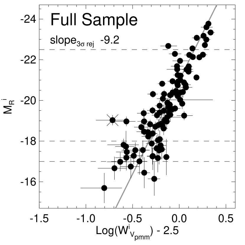
Figure 14: TFR for the full sample, including all morphologies and luminosities but restricted to $i>40$. Dashed lines indicate luminosity cuts used for Spearman rank tests (§8.1–8.2, see also §7.1). The gray line shows an unweighted inverse fit to all points, and the X marks a point automatically rejected by that fit as a $>$3$\sigma$ outlier.

As illustrated in Figure 15, scatter is dramatically higher for the full sample than for the spiral sample of §5–7. Including non-spiral and dwarf galaxies adds 0.77 mag of scatter in quadrature, yielding a total scatter of 1.07 mag. Faint non-spiral galaxies are responsible for most of the new scatter, so the relative importance of the morphology and luminosity extensions is unclear. The two E/S0’s brighter than M${}^{i}_{\rm R}=-20$ behave much like Sa galaxies, with a slight low $L$/high $W^{i}$ offset. Neistein et al. (1999) observe a similar TF offset for S0 galaxies using stellar kinematics.

Figure 15: Increase in TF scatter caused by extending the sample in morphology and luminosity. Scatter measurements are relative to an unweighted inverse fit. The full sample includes two emission-line galaxies of type E, whose inclinations may be unreliable. We include them for completeness, noting that one is very disky.

8.1 Physical Sources of Scatter in a Morphology-Blind TFR

We begin by broadening the spiral sample of §7 to include all morphologies, staying within the luminosity limits used in §7 (Table 2 and Figure 14) and as usual requiring $i>40$. In §8.2 we extend the luminosity range 1 mag fainter. Adding non-spirals brighter than M${}_{\rm R}^{i}=-18$ to the spiral sample strengthens the correlations between TF residuals and both rotation curve asymmetry and nuclear EW(H$\alpha$). We also see a hint of a new correlation between TF residuals and gas consumption timescale (based on incomplete data, as discussed in §7.2.6, but with 88% completeness for the newly added non-spiral galaxies). The TF residual–$\mu_{e}^{U}$ correlation remains about the same.

However, the expanded sample displays weaker correlations between TF residuals and both effective $B-R$ color and global (as opposed to nuclear) EW(H$\alpha$). As shown in Figure 16, the $(B-R)_{e}$ correlation actually falls below 3$\sigma$ at R. Although most non-spiral galaxies, marked with circled and boxed points in Figure 16, follow the correlation established by spiral galaxies quite well (albeit with slightly larger scatter), three of the six emission-line E/S0 galaxies in the sample are extreme outliers. These three outliers, labeled by name in Figure 16, have red colors $\gtrsim$1.2 and TF residuals $>$1 mag toward high $L$/low $W^{i}$. H I linewidths are available for two of the three S0 outliers; these two galaxies are clear outliers from the H I TFR as well, although the H I residuals are smaller than the optical RC residuals.

Figure 16: Correlation between TF residuals and $(B-R)_{e}^{i}$ color for galaxies of all morphologies in the range $-18<\rm M^{i}_{\rm R}<-22.5$. As before, we consider only galaxies with $i>40$. Boxed and circled points represent galaxies with morphological type later than Sd and earlier than Sa, respectively, which were not included in the spiral sample of §7. Most of these galaxies follow the spiral correlation well, except for three clear S0 outliers (discussed in §8.1). The Spearman rank probability of no correlation between $(B-R)_{e}^{i}$ and TF residuals in each optical band is given as $p_{band}$. Only R-band TF residuals are plotted.

The large TF residuals for these three S0 galaxies suggest that our observations do not accurately reflect their disk rotation velocities and/or their underlying luminosities. In each case the data are likely to be influenced by central activity, in the form of either an AGN or a central starburst. However, the central luminosity enhancements are too small to account for the TF offsets. Inclination errors are also unlikely to explain the outliers, as all three galaxies show disky morphologies and inclinations of $\sim$60-70 degrees. We suspect kinematic effects. NGC 4117 is a Seyfert II and has a truncated rotation curve that extends to only 0.56$r_{e}$; its stellar kinematics are peculiar and may indicate gas-stellar decoupling. A11332$+$3536 hosts a central starburst and has a truncated rotation curve that extends to 0.92$r_{e}$; the gas seems to lie in an inclined counterrotating disk (Kannappan & Fabricant, 2001). A12001$+$6439 has an unusually bright nucleus and its rotation curve reaches only 1.31$r_{e}$; the gas displays velocity reversals. For the latter two galaxies H I masses are available, from which we calculate rapid gas consumption timescales of $\sim$2 Gyr.

The irregular kinematics and starburst/AGN activity found in these S0 galaxies may result from recent interactions or mergers. As discussed by Barton & van Zee (2001), interacting galaxies may display radially truncated emission due to centrally concentrated starbursts, leading to artificially low velocity widths. Interactions and mergers can also generate non-coplanar gas and stellar rotation in early-type galaxies (Kannappan & Fabricant, 2001; Haynes et al., 2000), in which case artificially low gas velocities will be measured because the spectrograph slit P.A. is aligned to the stellar major axis rather than to the gas major axis. Deviations from the color–TF residual correlation provide a convenient and physically motivated way to identify such galaxies and prune them from a TF sample.

8.2 Physical Sources of Scatter in the Dwarf Extension of the TFR

Figure 17 plots third parameter–TF residual correlations for the full TF sample, with luminosity cuts extended to include dwarf galaxies down to M${}_{\rm R}^{i}=-17$ (see Table 2). Adding these dwarfs dilutes the third-parameter correlations for $(B-R)_{e}$ and EW(H$\alpha$) severely; for R-band TF residuals they become scatterplots. The only third-parameter correlations that reach 3$\sigma$ significance in the R band involve parameters that showed weak or nonexistent correlations for the spiral sample: rotation curve asymmetry, U-band effective surface brightness, and gas consumption timescale (see §7.2.4–7.2.6).

Figure 17: TF residuals vs. physical properties of the full sample (all morphologies, $i>40$, $-17<\rm M^{i}_{\rm R}<-22.5$, see §8.2 and Figure 14). Boxed and circled points represent galaxies with morphological type later than Sd and earlier than Sa, respectively, which were not included in the spiral sample of §7. (Other additional points are dwarf late-type spiral galaxies.) The Spearman rank probability of no correlation between the parameter and TF residuals in each optical band is given as $p_{band}$. Only R-band TF residuals are plotted.

Because these correlations are highly scattered, they are more easily understood in terms of bulk differences in properties for galaxies on either side of the TFR, rather than in terms of a linear trend like the color–TF residual correlation. Figure 18 illustrates these bulk differences with separate histograms for galaxies on either side of the TFR, considering only galaxies fainter than M${}_{\rm R}^{i}=-19$ since these galaxies are the primary drivers of the new correlations. (Unlike Figure 17, Figure 18 excludes galaxies with truncated rotation curves, which might appear on the low $W^{i}$ side of the TFR erroneously; however, Figure 18 applies no lower limit on luminosity.) In what follows we refer to galaxies fainter than M${}_{\rm R}^{i}=-19$ as “dwarfs.” Figure 15 shows that the non-spiral morphologies typical of dwarfs are most common below M${}_{\rm R}^{i}=-19$.

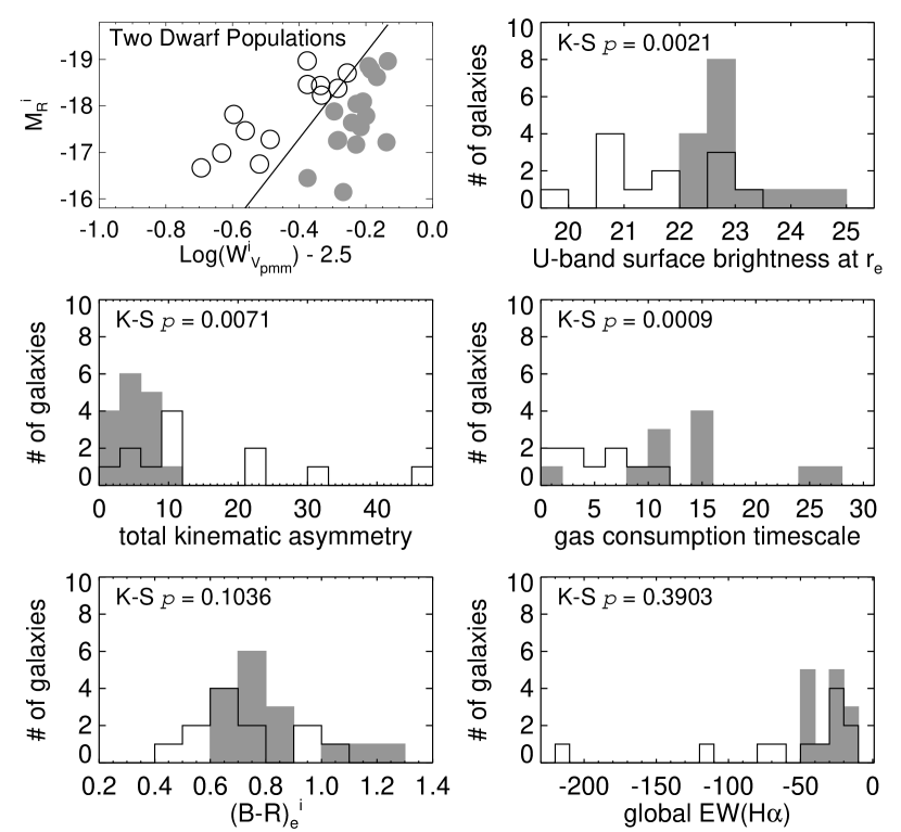
Figure 18: Physical properties of dwarf galaxies on either side of the TFR. Dwarfs on the high $W^{i}$/low $L$ side of the TFR are shown in gray, while those on the low $W^{i}$/high $L$ side are outlined in black. Each panel lists the Kolmogorov-Smirnov probability that the two sets of dwarfs were drawn from the same parent population with respect to the property shown. Here “dwarf” means anything fainter than M${}_{\rm R}^{i}=-19$; the luminosity cuts used for the third-parameter tests are not applied. Galaxies with truncated RCs ($<$1.3$r_{e}$) have been excluded from the figure because of uncertain location with respect to the TFR (however they do appear in Figure 17). Restoring these galaxies minimally affects the K-S test results for gas consumption timescale and U-band surface brightness but weakens the results for rotation curve asymmetry to 2$\sigma$ and eliminates any significant result for $B-R$ color. The reference TFR is the full sample TFR shown in Figure 14.

8.2.1 Rotation Curve Asymmetry

Asymmetries in rotation curves arise from multiple sources including turbulence, bars, tidal distortions, early or late-stage infall, and satellite accretion. Most of these underlying phenomena are likely to enhance star formation, qualitatively explaining the sense of the correlation in Figure 17 as well as its stronger statistical signal in bluer passbands. However, the scatter and substructure in the correlation suggest that the RC asymmetry–star formation connection may be complex. On the the high $L$/low $W^{i}$ side of the TFR, several dwarf galaxies show RC asymmetries $\gtrsim$10% (much higher than expected from the RC asymmetry–luminosity relation in Figure 11). On the other side of the TFR, RC asymmetries are generally lower and more uniform (Figure 18; see also §8.3).

8.2.2 U-Band Effective Surface Brightness

If U-band effective surface brightness ($\mu_{e}^{U}$) measures the surface density of recent star formation in galaxy disks, then high $\mu_{e}^{U}$ (numerically small values) should correlate with high global star formation activity, consistent with the observed TF residual–$\mu_{e}^{U}$ correlation. However this view may be too simplistic, because galaxies ranging from undisturbed spirals to emission-line S0’s with kinematically decoupled gas all seem to follow the same correlation, albeit with very large scatter. Given the constancy of the Spearman test significance for this correlation whether using U, B, or R-band TF residuals (Figure 17), we suggest that variations in $\mu_{e}^{U}$ may track not only star formation but also structural differences between classes of galaxies located in different parts of the $L$–$W^{i}$ plane, such as differences in the concentration of light or the velocity width at a given luminosity. Dwarfs on opposite sides of the TFR have different $\mu_{e}^{U}$ distributions (Figure 18), analogous to the different rotation curve asymmetry distributions discussed in the previous section. While low to moderate surface brightnesses occur on both sides of the TFR, high surface brightnesses occur only on the high $L$/low $W^{i}$ side.

8.2.3 Gas Consumption Timescale

Typical gas consumption timescales also appear to differ for dwarfs on the two sides the TFR, although this result relies on incomplete H I mass data (82% complete for the galaxies in Figure 18, with fainter galaxies preferentially missing). In Figures 17 and 18, only a few galaxies have low $L$/high $W^{i}$ (positive) residuals and very short gas consumption timescales. By contrast, short gas consumption timescales are the norm for galaxies with negative residuals. Most of the latter set are low-luminosity non-spiral galaxies, which explains the emergence of a gas consumption timescale correlation in the full sample, where there was no correlation in the spiral sample of §7.

8.3 Is the Dwarf Split Real?

In §8.2.1–8.2.3 we showed that if we divide the dwarf population into two groups with positive and negative offsets from the TFR, the groups have distinct physical properties (summarized in Figure 18). Although K-S tests yield only $\sim$3$\sigma$ confidence that the two populations are distinct based on any one property, the same split is observed for three completely independent parameters: rotation curve asymmetry (based on high-resolution spectra), $\mu_{e}^{U}$ (based on surface photometry), and gas consumption timescale (based on catalog H I data and NFGS spectrophotometry). The TF residuals for the two dwarf populations differ by $\sim$2 mag in the mean.

We now consider whether systematic effects might create such a split. Because the two sets of dwarfs in Figure 18 show similar distributions in inclination and morphology, correlated inclination errors are unlikely. Truncated optical RCs are also unlikely to play a role, as Figure 18 excludes galaxies whose RCs do not reach 1.3$r_{e}$. Furthermore, replacing optical velocity widths with H I linewidths preserves the division. RC asymmetries may affect measured velocity widths, but the asymmetries we measure are too small to produce a 2 mag difference between the two groups of dwarfs (cf. §7.3.2).

Correlated distance errors might be a concern. Both dwarf populations show broad distributions in R.A.-Dec.-redshift space, but due to the NFGS selection procedure, the two sets of dwarfs in Figure 18 have systematically different recession velocities: 500–1300 and 700–1600 $\rm km\,s^{-1}$ for underluminous and overluminous dwarfs respectively, with over half the underluminous set in the range 500–700 $\rm km\,s^{-1}$ (measured with respect to the Local Group). To test whether peculiar velocities or local flows may have affected our distance estimates and produced a spurious bifurcation in luminosities, we have substituted distances estimated by a number of techniques. These include: (1) Hubble-law distances assigned using group recession velocities rather than individual galaxy recession velocities (Tully, 1988; Tully et al., 1992); (2) absolute distances derived from the light-to-mass model of Tully et al. (1992); (3) Hubble-law distances with and without corrections for Virgocentric infall (§4.1) and/or for the Local Anomaly (Han & Mould, 1990). The segregation of the two dwarf populations is robust under all of these substitutions, with the caveat that many of the overluminous (low velocity width) dwarf galaxies lack distances from methods (1) and (2).

We conclude that the TF offset between the two groups of NFGS dwarfs is probably real. These results confirm trends reported for two other heterogeneous TF samples (Stil & Israel, 1998; Pierini, 1999). Both studies identify a rotationally supported dwarf population on the faint side of the TFR and a population with comparable rotational and random velocities on the bright side (where we measure high rotation curve asymmetries).

The physical mechanisms responsible for the disturbed kinematics and rapid gas consumption of the dwarfs on the bright side of the TFR are uncertain, but interactions are an obvious possibility. Without deep wide-field imaging we cannot evaluate the frequency of close companions for the two populations, particularly given the possibility of relatively faint neighbors. Nonetheless, it is intriguing to note that deep survey work by Taylor et al. (1996) has demonstrated a statistically higher rate of companions near starbursting dwarfs than near LSB dwarfs (see also Pustilnik et al., 2001). The analogy is suggestive rather than exact, as our two dwarf populations do not show a definitive split in EW(H$\alpha$), although the three most extreme starbursting dwarfs do fall on the bright side of the TFR (Figure 18).

8.4 Dwarfs in Ursa Major

The three studies that have reported a difference in dwarf properties on either side of the TFR are all based on heterogeneous galaxy samples representing a variety of environments (our own; Stil & Israel, 1998; Pierini, 1999). Here we investigate dwarf properties and their relationship to the TFR for the Ursa Major sample of Verheijen & Sancisi (2001), which represents a single moderate-density environment. While the VS data set does not include kinematic asymmetries or U-band data, we can examine B-band surface brightnesses and TF offsets. (Although not significant at the 3$\sigma$ level, $\mu_{e}^{B}$ trends basically follow $\mu_{e}^{U}$ trends with weaker signal.)

As noted in §5.3 (see also Figure 6), the Ursa Major TFR appears to diverge from the NFGS TFR at the faint end. When we expand the two spiral samples to include late-type galaxies and dwarfs down to M${}_{\rm B}=-16.8$ (the Ursa Major sample completeness limit), we find a TF offset of $\sim$0.5 mag between the NFGS and Ursa Major dwarfs, with the Ursa Major dwarfs showing higher $L$/lower $W^{i}$. For the same NFGS and Ursa Major dwarfs, we also find a mean effective surface brightness ($\mu_{e}^{B}$) offset of $\sim$0.5 mag arcsec^-2, with the Ursa Major dwarfs fainter. These results do not conform to what we observe in the NFGS, where overluminous dwarfs have relatively bright $\mu_{e}^{B}$ values. Also, Figure 19 shows that the Ursa Major dwarfs display a very narrow range in $\mu_{e}^{B}$ compared to the NFGS, with a faint median value of 23.7. Herein lies a possible explanation for the discrepancy: if LSB dwarfs are more likely to have rising RCs at their outermost observed radii, then the “true” halo velocities of the Ursa Major dwarfs may be systematically underestimated (cf. Verheijen, 2001).

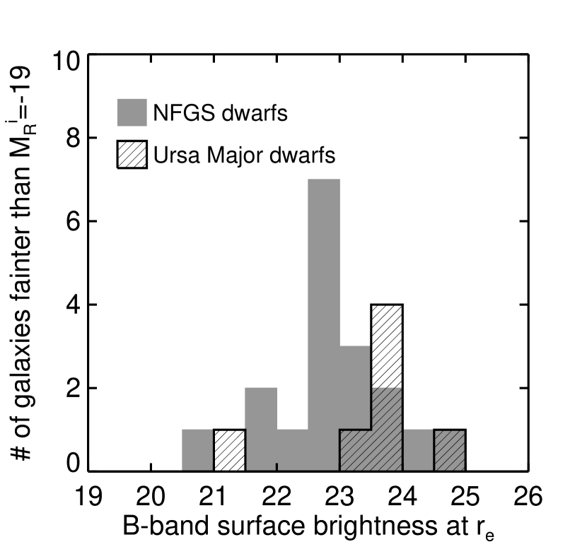
Figure 19: Comparison of B-band effective surface brightnesses for the NFGS and Ursa Major dwarfs that meet the TF sample criteria described in §8.4. To match the Ursa Major sample completeness limit (M${}_{\rm B}=-16.8$), the figure omits many of the fainter NFGS galaxies included in §8.2. We measure $\mu_{e}^{B}$ for the Ursa Major galaxies directly from the profiles given in Tully et al. (1996), using the effective radii listed in their Table 4 and the Dexter java applet in the ADS (NASA’s Astrophysics Data System). The measured values are corrected for a small mean offset (0.2 mag arcsec^-2) determined by comparing $\mu_{e}^{B}$ values for six galaxies common to both the NFGS and Ursa Major databases; without this correction the dwarf surface brightness offset shown in the figure would be smaller.

In this case the divergence of the two TFRs may be due to real physical differences between the two dwarf populations, and the narrow range of properties seen for the Ursa Major dwarfs may simply reflect the specific environment of Ursa Major. The cluster consists of a moderate overdensity of spiral galaxies that lacks any discernible core, contains no elliptical galaxies, and includes surprisingly few dwarfs relative to bright galaxies (Tully et al., 1996; Trentham et al., 2001). Trentham et al. (2001) infer from the scarcity of dwarf galaxies in Ursa Major that the cluster collapsed late, so that its dwarf halos formed after reionization when conditions were poor for star formation.

Nonetheless, the environmental differences hypothesis should be treated with caution, because the Ursa Major dwarfs differ from those in the NFGS at only the 2$\sigma$ level, with velocity width data missing for a few dwarfs and with the cluster membership of another dwarf in question (see note 5; this galaxy happens to appear in both data sets). Furthermore, we cannot completely eliminate small systematic uncertainties in relative distance scale and photometric calibration between the two data sets; a larger and more uniform data set would be required to definitively establish the existence of environmental effects.

8.5 Two Dwarf Galaxy Populations and the Slope of the TFR

As noted by Pierini (1999), the existence of two dwarf populations complicates TF slope measurements. For the full sample, we find a linear TF slope with no break at low luminosities (top left panel of Figure 20). However, different sample selection criteria may favor one dwarf population over the other, with consequences for the faint-end slope.

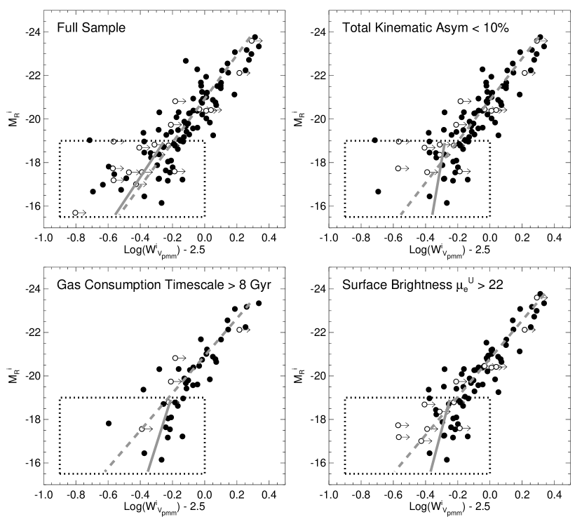
Figure 20: Effects of sample selection on the faint-end slope of the TFR. Each panel shows galaxies that meet the selection criterion indicated and have inclinations $i>40$. Arrows mark galaxies whose rotation curves are truncated at less than 1.3$r_{e}$; these galaxies may have velocity widths larger than we measure. The dashed and solid gray lines show the TFR for galaxies brighter and fainter than M${}_{\rm R}^{i}=-19$, respectively; the dashed line determined by the brighter galaxies extends into the box for reference only.

If we consider the TFR as a physical rather than an empirical relation, linking luminosity and rotation velocity for passively evolving disk galaxies, then we should restrict it to undisturbed rotationally supported systems. Dwarf galaxies on the low $L$/high $W^{i}$ side of the TFR best meet this description. These galaxies show moderate rotation curve asymmetries, indicating that they are probably rotationally supported. In addition, their long gas consumption timescales and low U-band effective surface brightnesses appear consistent with quiescent evolution. (We note that photometric “normalcy” is not a useful criterion for dwarfs, as almost all are lumpy and asymmetric, so defining what is “peculiar” becomes extremely difficult.)

Figure 20 demonstrates the effect of selecting restricted TF samples to match the properties of the quiescent dwarfs at all luminosities. Each panel shows separate TF fits for galaxies above and below M${}_{\rm R}^{i}=-19$, first for the full TF sample, and then for subsamples restricted in turn to have low kinematic asymmetry, long gas consumption timescale, and faint U-band effective surface brightness. The faint-end fits should not be interpreted as precisely measuring the slope of the dwarf TFR, given the small number statistics and short lever arm. Nonetheless, these fits clearly suggest a faint-end slope discontinuity for TF samples restricted to undisturbed, rotationally supported galaxies: the dwarfs in these samples appear underluminous when compared to the extrapolated bright-galaxy TFR.

Breaks in the faint-end slope of the TFR have been previously observed for extremely late type spirals (Matthews et al., 1998) and LSB dwarfs (McGaugh et al., 2000). McGaugh et al. demonstrate that a straight TF slope (the “baryonic Tully-Fisher relation”) can be restored for LSB dwarfs by mathematically converting their gas into stars and correcting the luminosity for these unformed stars. This procedure does not work very well for our faint galaxies, but McGaugh et al. see significant effects primarily for galaxies fainter than our cutoff of M${}_{\rm R}^{i}\sim-16$.

9 Conclusions

The Nearby Field Galaxy Survey offers an ideal sample for exploring the link between offsets from the Tully-Fisher relation and the evolutionary states of galaxies. Galaxies in the NFGS were selected from the CfA 1 redshift survey without preference for morphology or environment and span a wide range of luminosities, $-23<\rm M_{\rm B}<-15$. Using UBR photometry, optical rotation curve data, and H I linewidths, we have analyzed TF residuals for two subsamples of the NFGS, a sample of Sa–Sd galaxies brighter than $\rm M_{\rm R}^{i}=-18$ and an extended sample including dwarfs and non-spiral galaxies.

Within the spiral sample, we find strong third-parameter correlations between TF residuals and both $B-R$ color and EW(H$\alpha$). The cleanest correlations are achieved using effective colors (measured within the effective radius) and global equivalent widths of H$\alpha$ and [OII] (integrated over the entire galaxy). Using the color–TF residual correlation in each TF band to define a color-correction term to the TFR, we reduce scatter to a single constant value across the R, B, and U bands, eliminating the usual trend of increasing scatter with bluer passbands. The remaining scatter of $\sim$0.65 mag (at a slope of $-$10) approximately equals the scatter we expect from measurement errors. An EW(H$\alpha$)-correction term performs equally well for the R and B-band TFRs and almost as well for the U-band TFR.

The color and EW(H$\alpha$) correlations are continuous, but their statistical signal is strongly driven by two morphology classes: peculiar galaxies (by which we mean recognizable spiral galaxies with oddities such as warps, multiple nuclei, or interacting companions) that fall on the high luminosity/low velocity width side of the TFR, and Sa galaxies that fall on the low luminosity/high velocity width side of the TFR. This result offers a different perspective on the longstanding debate over the Sa offset, by linking the offset simply to the fact that Sa galaxies are consistently red.

Differences in star formation history offer the simplest explanation for the color–TF residual correlation: as stellar populations evolve, changes in their colors and luminosities are intimately connected. We argue that the steep slope of the correlation cannot be explained in terms of a trivial correlation due to passband-dependent scatter. Interpreting TF residuals as luminosity residuals, the slope of the color–TF residual correlation can be directly compared with the predictions of population synthesis models of disk galaxy evolution. The slopes we find using R and B band TF residuals closely match the slopes predicted from the passively evolving galaxy models of Bell & de Jong (2001). However, we find a slight suggestion of steeper slopes, which might be taken as evidence that in addition to passive evolution, many spiral galaxies experience significant starburst-driven evolution, e.g. triggered by interactions or minor mergers (as independently suggested by the disturbed morphology and kinematics of many of our bluer galaxies). Variations in dark matter structure could also steepen the correlation if they were correlated with color, although we find no independent evidence for such an effect. Finally, the present data set cannot conclusively rule out systematic trends caused by kinematic distortions or inclination errors that correlate with galaxy color: such trends are unlikely to explain the entire color–TF residual correlation but may affect its slope.

Removing the spiral morphology restriction, we find that most non-spiral galaxies brighter than $\rm M_{\rm R}^{i}=-18$ follow the color–TF residual and EW(H$\alpha$)–TF residual correlations established by spiral galaxies, but with greater scatter. A few emission-line S0 galaxies at the faint end of the included range deviate strongly from both the TFR and the color–TF residual correlation; these galaxies all show starburst or AGN activity and anomalous gas kinematics.

Dwarf galaxies fainter than $\sim\rm M_{\rm R}^{i}=-18$ do not follow the color–TF residual correlation. However, dwarfs on the high luminosity/low velocity width side of the TFR have higher rotation curve asymmetries, higher U-band effective surface brightnesses, and shorter gas consumption timescales than dwarfs on the low luminosity/high velocity width side of the TFR. These properties suggest that many of the high $L$/low $V$ dwarfs are “disturbed,” while the low $L$/high $V$ dwarfs are likely to be passively evolving, rotationally supported systems.

This split in dwarf properties implies that the faint-end slope of the TFR depends on sample selection. We find no break in slope for dwarf galaxies in the full NFGS sample. However, if we select for rotationally supported, passively evolving galaxies at all luminosities, we find evidence for a break toward steeper slope at the faint end of the TFR, consistent with recent work by Matthews et al. (1998) and McGaugh et al. (2000).

Appendix A Tully-Fisher Fitting Technique

TF samples are generally incomplete at low luminosities and low surface brightnesses, resulting in asymmetric scatter about the fundamental relation. In a fit to magnitude as a function of $\log v$ (the “forward” TFR), this asymmetric scatter leads to artificially shallow slopes. Extended luminosity coverage, as in the NFGS, helps to alleviate the problem, but asymmetric faint-end scatter can still bias results.

Willick (1994) describes one way to address TF slope bias, using an iterative analysis. His technique assumes that the “missing” galaxies have the same intrinsic TF slope and scatter as the observed galaxies. However, if either the scatter or the slope increases at low luminosity, the bias-corrected slope is still too shallow.

Alternatively, one can fit the “inverse” relation (minimizing the scatter in velocity width as a function of magnitude) without any bias correction, assuming that velocity width biases are negligible (cf. Tully & Pierce, 2000; Schechter, 1980). This approach seems appropriate for our sample, because: (1) optical RC data (unlike radio data) are not subject to a velocity width detection bias, and (2) the NFGS makes no explicit diameter cut that might introduce an indirect velocity width bias through a correlation of rotation speed with surface brightness. However, intrinsic surface brightness and color bias in the parent survey may still play a role.

Tables 1 and 2 present our basic TF calibrations using three different techniques: error-weighted inverse fits, bivariate fits with regression in both magnitude and velocity width errors, and unweighted inverse fits, our preferred technique. Error-weighted inverse fits avoid the usual TF slope bias, but they favor galaxies with higher luminosity and larger velocity width, which have smaller errors. Bivariate fits use all the available information but at the expense of introducing some slope bias (c.f.  Sakai et al., 2000). Note that the systematic differences between these fitting techniques often exceed the formal errors (Tables 1 and 2).

We compute unweighted inverse fits in two steps. First we find the 68% confidence interval for the slope, where for each test value of the slope we allow the intercept to assume the value that minimizes deviations for that slope. Once we have the best-fit slope, we fit for the intercept with the slope fixed. Although the results are the same as those of a one-step two-parameter fit, the errors are different. This type of fit is appropriate for comparing the slopes of different samples irrespective of zero point, or conversely for comparing their zero points at fixed slope.

All fits are subject to one round of 3$\sigma$ rejection. Such rejection reduces measured scatter in a Gaussian distribution by $\sim$2%, which we correct for in $\sigma_{3\sigma\,\rm rej}$. Using the same slope and zero point we also compute the full scatter $\sigma_{\rm all\,pts}$, the biweight scatter (Beers et al., 1990), and the predicted scatter from observational errors $\sigma_{\rm pred}$. The biweight statistic provides the most robust measure of observed scatter, generally agreeing closely with $\sigma_{3\sigma\,\rm rej}$.

Appendix B Velocity Width Definitions & Optical-To-Radio Conversions

Below we present three different optical velocity width definitions, $V_{max}$, $V_{fit}$, and $V_{pmm}$, and place them on an equivalent W₅₀ scale. Our optical-to-radio conversions are expected to differ from those of Courteau (1997), not just because of differences in sample selection, but also because Courteau’s conversions are calibrated using turbulence-corrected H I linewidths (taken from Giovanelli et al., 1997b). In our case, the conversions are calibrated using uncorrected H I linewidths.

B.1 $V_{max}$

We define $V_{max}$ as the single largest velocity in the rotation curve, relative to the origin defined by minimizing the RC asymmetry (Appendix C). Because this number does not make use of the full information in the rotation curve, we expect it to be somewhat unreliable. Nonetheless, it correlates surprisingly well with the radio linewidth W₅₀ (Figure 21), even when the optical RC does not extend as far as 1.3$r_{e}$ Freeman (the peak velocity position for an exponential disk with effective radius $r_{e}$, 1970). An iterative least-squares fit with automatic 3.5$\sigma$ outlier rejection yields

$$\rm W_{50}=19\left(\pm 6\right)+0.90\left(\pm 0.03\right)\left(2V_{max}\right)$$ (B1)

with scatter 25 $\rm km\,s^{-1}$.

Figure 21: W₅₀ versus $V_{max}$, $V_{fit}$, and $V_{pmm}$ for the 96 galaxies with both optical RC and H I W₅₀ velocity widths. Boxes indicate points for which the optical rotation curve does not extend to 1.3$r_{e}$; remarkably, these points show no strong deviation from the general correlation. Lines indicate least squares fits to the data with automatically rejected points ($>$3.5$\sigma$) marked by an X. All three X’s represent galaxies currently interacting with another galaxy: NGC 4795, NGC 7752, and NGC 2799. The open-circle points mark galaxies with potentially large position angle misalignment in the optical RC data (§3.2); these are also excluded from the fit. The zero point offset indicates the nonzero contribution of turbulence to the H I profiles even at zero rotation velocity.

B.2 $V_{fit}$

Following Courteau (1997), we define $V_{fit}$ by first fitting the empirical function

$$v=v_{0}+v_{c}\frac{(1+x)^{\beta}}{(1+x^{\gamma})^{1/\gamma}}$$ (B2)

to the observed RC, with the origin unconstrained, and then interpolating to find the velocity at a specific radius. Here $x=r_{t}/(r-r_{0})$, $(r_{0},v_{0})$ defines the origin, $v_{c}$ gives the velocity scale, $r_{t}$ is related to the turnover radius, and $\gamma$ and $\beta$ are free parameters governing the shape of the rotation curve. We modify Courteau’s technique slightly, in that we interpolate the velocity $V_{fit}$ at 1.3$r_{e}$ rather than at 2.2 disk scale lengths $r_{d}$, because 1.3$r_{e}$ remains well defined even for non-disk galaxies and does not require bulge+disk decomposition. Theoretically the two radii are equivalent, in that both represent the peak velocity position for a pure exponential disk (Freeman, 1970). For disk-dominated galaxies in the NFGS, 1.3$r_{e}$ and 2.2$r_{d}$ also match well observationally. (Disk scale lengths are courtesy of R. Jansen, private communication; both disk scale lengths and $r_{e}$’s are from the B band images of Jansen et al. (2000b).)

As shown in Figure 4, our modified-Courteau technique performs well for bright spiral galaxies comparable to those in Courteau’s sample, but less regular RCs are poorly modeled. Figure 21 displays the correlation of $V_{fit}$ with the radio linewidth W₅₀, demonstrating reasonable agreement, although some points are simply missing because the fit would not converge. An iterative least-squares fit with automatic 3.5$\sigma$ outlier rejection yields

$$\rm W_{50}=45\left(\pm 5\right)+0.90\left(\pm 0.03\right)\left(2V_{fit}\right).$$ (B3)

We define the equivalent W₅₀ linewidth W${}_{V_{fit}}$ by this equation and assign it an error equal to the scatter in the fit, 25 $\rm km\,s^{-1}$.

B.3 $V_{pmm}$

Following Raychaudhury et al. (1997), we define $V_{pmm}$ as half the difference between the statistical “probable maximum” and “probable minimum” velocities implied by the observed rotation curve. The probable maximum velocity $v_{pmax}$ is defined to have a 10 percent chance of exceeding all velocities in the rotation curve:

$$\prod_{i}P\left(v_{pmax}>v_{i}\right)=0.1.$$ (B4)

Modeling each velocity $v_{i}$ as a Gaussian distribution about the measured value, with $\sigma$ equal to the measurement error, we obtain

$$\prod_{i}\left(\frac{1}{2}+\frac{1}{2}{\rm erf}{\frac{v_{pmax}-v_{i}}{\sqrt{2}\sigma_{i}}}\right)=0.1,$$ (B5)

which may be solved numerically for $v_{pmax}$. The probable minimum velocity $v_{pmin}$ is defined by analogy, and $2V_{pmm}=v_{pmax}-v_{pmin}$.

Courteau (1997) suggests that $V_{pmm}$ will be very sensitive to outlying points in the rotation curve, while Raychaudhury et al. (1997) claim the opposite. The difference seems to hinge on the size of the error bars associated with the outliers — if a high S/N cosmic ray hit masquerades as a very high-velocity data point, it may indeed throw off $V_{pmm}$, but outlying points with large error bars will have relatively little impact. In practice, $V_{pmm}$ produces smaller scatter than $V_{fit}$ in the optical-to-H I conversion. More importantly, as Raychaudhury et al. point out, $V_{pmm}$ has the virtue of using all of the data in the rotation curve without imposing any particular model on the data. The diversity of the NFGS defies modeling through a simple fitting function (see Figure 4).

Figure 21 shows the correlation of $V_{pmm}$ with radio linewidth W₅₀. An iterative least-squares fit with automatic 3.5$\sigma$ outlier rejection yields

$$\rm W_{50}=33\left(\pm 5\right)+0.92\left(\pm 0.02\right)\left(2V_{pmm}\right).$$ (B6)

We define the equivalent W₅₀ linewidth W${}_{V_{pmm}}$ by this equation and assign it an error equal to the scatter in the fit, 20 $\rm km\,s^{-1}$.

Appendix C Rotation Curve Asymmetry Measurements

We compute optical rotation curve asymmetries using a technique similar to the photometric technique of Abraham et al. (1996). Reflecting the rest-frame rotation curve about its origin, we find the average absolute deviation between the two sides, $<\mid\!v-v^{\rm reflected}\!\mid>$, and express the result as a percentage of the velocity width $2V_{pmm}$ (Appendix B.3). Our asymmetry, velocity width, and central redshift measurements are not completely independent of one another, therefore in practice we perform these calculations iteratively.

Asymmetry measurements depend sensitively on the choice of origin for the spatial and velocity axes. We therefore vary the position of the origin to minimize the asymmetry, keeping the spatial coordinate constrained within the one-sigma error bars of the continuum peak position, while allowing the velocity coordinate to vary freely. At each step in the minimization process we resample the rotation curve onto a uniform spatial grid about the trial origin.

To partially standardize our asymmetry index for rotation curves of differing spatial extent, we define an inner asymmetry using only points within 1.3$r_{e}$ (the peak velocity position for a pure exponential disk, Appendix B.2). When the rotation curve does not extend this far, we compute the inner asymmetry from the data available. The rotation curve origin is determined by minimizing the inner asymmetry. All other analysis makes use of the total asymmetry, which we compute relative to the origin defined by minimizing the inner asymmetry.

References

- Aaronson et al. (1982) Aaronson, M., Huchra, J., Mould, J., Schechter, P. L., & Tully, R. B. 1982, ApJ, 258, 64
- Abraham et al. (1996) Abraham, R. G., Tanvir, N. R., Santiago, B. X., Ellis, R. S., Glazebrook, K., & van den Bergh, S. 1996, MNRAS, 279, L47
- Barton et al. (2001) Barton, E. J., Geller, M. J., Bromley, B. C., van Zee, L., & Kenyon, S. J. 2001, AJ, 121, 625
- Barton & van Zee (2001) Barton, E. J. & van Zee, L. 2001, ApJ, 550, L35
- Beers et al. (1990) Beers, T. C., Flynn, K., & Gebhardt, K. 1990, AJ, 100, 32
- Bell & de Jong (2001) Bell, E. F. & de Jong, R. S. 2001, ApJ, 550, 212
- Bershady & Andersen (2000) Bershady, M. A. & Andersen, D. R. 2000, in ASP Conf. Ser. 197: Dynamics of Galaxies: from the Early Universe to the Present, 175
- Bershady et al. (1999) Bershady, M. A., Haynes, M. P., Giovanelli, R., & Andersen, D. R. 1999, in ASP Conf. Ser. 182: Galaxy Dynamics - A Rutgers Symposium, 499
- Bottinelli et al. (1990) Bottinelli, L., Gouguenheim, L., Fouque, P., & Paturel, G. 1990, A&AS, 82, 391
- Buchalter et al. (2001) Buchalter, A., Jimenez, R., & Kamionkowski, M. 2001, MNRAS, 322, 43
- Bureau et al. (1996) Bureau, M., Mould, J. R., & Staveley-Smith, L. 1996, ApJ, 463, 60
- Courteau (1996) Courteau, S. 1996, ApJS, 103, 363
- Courteau (1997) —. 1997, AJ, 114, 2402
- Courteau & Rix (1999) Courteau, S. . & Rix, H. 1999, ApJ, 513, 561
- Eisenstein & Loeb (1996) Eisenstein, D. J. & Loeb, A. 1996, ApJ, 459, 432
- Elizondo et al. (1999) Elizondo, D., Yepes, G., Kates, R., Müller, V., & Klypin, A. 1999, ApJ, 515, 525
- Fabricant et al. (1998) Fabricant, D., Cheimets, P., Caldwell, N., & Geary, J. 1998, PASP, 110, 79
- Forbes et al. (1996) Forbes, D. A., Phillips, A. C., Koo, D. C., & Illingworth, G. D. 1996, ApJ, 462, 89
- Franx & de Zeeuw (1992) Franx, M. & de Zeeuw, T. 1992, ApJ, 392, L47
- Freeman (1970) Freeman, K. C. 1970, ApJ, 160, 811
- Frei & Gunn (1994) Frei, Z. & Gunn, J. E. 1994, AJ, 108, 1476
- Garnier et al. (1996) Garnier, R., Paturel, G., Petit, C., Marthinet, M. C., & Rousseau, J. 1996, A&AS, 117, 467
- Giovanelli et al. (1997a) Giovanelli, R., Haynes, M. P., Herter, T., Vogt, N. P., da Costa, L. N., Freudling, W., Salzer, J. J., & Wegner, G. 1997a, AJ, 113, 53
- Giovanelli et al. (1997b) Giovanelli, R., Haynes, M. P., Herter, T., Vogt, N. P., Wegner, G., Salzer, J. J., da Costa, L. N., & Freudling, W. 1997b, AJ, 113, 22
- Giraud (1986) Giraud, E. 1986, A&A, 164, 17
- Gordon et al. (1997) Gordon, K. D., Calzetti, D., & Witt, A. N. 1997, ApJ, 487, 625
- Han & Mould (1990) Han, M. & Mould, J. 1990, ApJ, 360, 448
- Haynes et al. (1999) Haynes, M. P., Giovanelli, R., Chamaraux, P., da Costa, L. N., Freudling, W., Salzer, J. J., & Wegner, G. 1999, AJ, 117, 2039
- Haynes et al. (2000) Haynes, M. P., Jore, K. P., Barrett, E. A., Broeils, A. H., & Murray, B. M. 2000, AJ, 120, 703
- Huchra et al. (1983) Huchra, J., Davis, M., Latham, D., & Tonry, J. 1983, ApJS, 52, 89
- Isobe et al. (1990) Isobe, T., Feigelson, E. D., Akritas, M. G., & Babu, G. J. 1990, ApJ, 364, 104
- Jacoby et al. (1992) Jacoby, G. H., Branch, D., Clardullo, R., Davies, R. L., Harris, W. E., Pierce, M. J., Pritchet, C. J., Tonry, J. L., & Welch, D. L. 1992, PASP, 104, 599
- Jansen (2000) Jansen, R. A. 2000, PhD thesis, Univ. Groningen, The Netherlands
- Jansen et al. (2000a) Jansen, R. A., Fabricant, D., Franx, M., & Caldwell, N. 2000a, ApJS, 126, 331
- Jansen et al. (2000b) Jansen, R. A., Franx, M., Fabricant, D., & Caldwell, N. 2000b, ApJS, 126, 271
- Jorgensen (1994) Jorgensen, I. 1994, PASP, 106, 967
- Kannappan (2001) Kannappan, S. J. 2001, PhD thesis, Harvard University
- Kannappan & Fabricant (2001) Kannappan, S. J. & Fabricant, D. G. 2001, AJ, 121, 140
- Kennicutt (1998) Kennicutt, R. C., J. 1998, ARA&A, 36, 189
- Kennicutt et al. (1994) Kennicutt, R. C., J., Tamblyn, P., & Congdon, C. E. 1994, ApJ, 435, 22
- Kodaira & Watanabe (1988) Kodaira, K. & Watanabe, M. 1988, AJ, 96, 1593
- Kraan-Korteweg et al. (1984) Kraan-Korteweg, R. C., Sandage, A., & Tammann, G. A. 1984, ApJ, 283, 24
- Marzke et al. (1994) Marzke, R. O., Huchra, J. P., & Geller, M. J. 1994, ApJ, 428, 43
- Mathewson et al. (1992) Mathewson, D. S., Ford, V. L., & Buchhorn, M. 1992, ApJS, 81, 413
- Matthews et al. (1998) Matthews, L. D., van Driel, W., & Gallagher, J. S. 1998, AJ, 116, 2196
- McGaugh et al. (2000) McGaugh, S. S., Schombert, J. M., Bothun, G. D., & de Blok, W. J. G. 2000, ApJ, 533, L99
- Mihos & Hernquist (1996) Mihos, J. C. & Hernquist, L. 1996, ApJ, 464, 641
- Neistein et al. (1999) Neistein, E., Maoz, D., Rix, H., & Tonry, J. L. 1999, AJ, 117, 2666
- Nilson (1973) Nilson, P. 1973, Uppsala general catalogue of galaxies (Uppsala: Astronomiska Observatorium, 1973)
- O’Neil et al. (2000) O’Neil, K., Bothun, G. D., & Schombert, J. 2000, AJ, 119, 136
- Pierce & Tully (1988) Pierce, M. J. & Tully, R. B. 1988, ApJ, 330, 579
- Pierce & Tully (1992) —. 1992, ApJ, 387, 47
- Pierini (1999) Pierini, D. 1999, A&A, 352, 49
- Pierini & Tuffs (1999) Pierini, D. & Tuffs, R. J. 1999, A&A, 343, 751
- Pustilnik et al. (2001) Pustilnik, S. A., Kniazev, A. Y., Lipovetsky, V. A., & Ugryumov, A. V. 2001, A&A, 373, 24
- Raychaudhury et al. (1997) Raychaudhury, S., von Braun, K., Bernstein, G. M., & Guhathakurta, P. 1997, AJ, 113, 2046
- Rhee (1996) Rhee, M.-H. 1996, PhD thesis, Univ. Groningen, The Netherlands
- Rix et al. (1997) Rix, H., Guhathakurta, P., Colless, M., & Ing, K. 1997, MNRAS, 285, 779
- Roberts (1978) Roberts, M. S. 1978, AJ, 83, 1026
- Rubin et al. (1985) Rubin, V. C., Burstein, D., Ford, W. K., & Thonnard, N. 1985, ApJ, 289, 81
- Sakai et al. (2000) Sakai, S., Mould, J. R., Hughes, S. M. G., Huchra, J. P., Macri, L. M., Kennicutt, R. C., Gibson, B. K., Ferrarese, L., Freedman, W. L., Han, M., Ford, H. C., Graham, J. A., Illingworth, G. D., Kelson, D. D., Madore, B. F., Sebo, K., Silbermann, N. A., & Stetson, P. B. 2000, ApJ, 529, 698
- Schechter (1980) Schechter, P. L. 1980, AJ, 85, 801
- Simard & Pritchet (1998) Simard, L. & Pritchet, C. J. 1998, ApJ, 505, 96
- Stil & Israel (1998) Stil, J. M. & Israel, F. P. 1998, in astro-ph/9810151
- Strauss & Willick (1995) Strauss, M. A. & Willick, J. A. 1995, Phys. Rep., 261, 271
- Taylor et al. (1996) Taylor, C. L., Thomas, D. L., Brinks, E., & Skillman, E. D. 1996, ApJS, 107, 143
- Theureau et al. (1998) Theureau, G., Bottinelli, L., Coudreau-Durand, N., Gouguenheim, L., Hallet, N., Loulergue, M., Paturel, G., & Teerikorpi, P. 1998, A&AS, 130, 333
- Trentham et al. (2001) Trentham, N., Tully, R. B., & Verheijen, M. A. W. 2001, MNRAS, 325, 385
- Tully (1988) Tully, R. B. 1988, Nearby galaxies catalog (Cambridge and New York, Cambridge University Press)
- Tully & Fisher (1977) Tully, R. B. & Fisher, J. R. 1977, A&A, 54, 661
- Tully & Fouque (1985) Tully, R. B. & Fouque, P. 1985, ApJS, 58, 67
- Tully & Pierce (2000) Tully, R. B. & Pierce, M. J. 2000, ApJ, 533, 744
- Tully et al. (1998) Tully, R. B., Pierce, M. J., Huang, J., Saunders, W., Verheijen, M. A. W., & Witchalls, P. L. 1998, AJ, 115, 2264
- Tully et al. (1992) Tully, R. B., Shaya, E. J., & Pierce, M. J. 1992, ApJS, 80, 479
- Tully et al. (1996) Tully, R. B., Verheijen, M. A. W., Pierce, M. J., Huang, J., & Wainscoat, R. J. 1996, AJ, 112, 2471
- Tutui & Sofue (1997) Tutui, Y. & Sofue, Y. 1997, A&A, 326, 915
- Verheijen (1997) Verheijen, M. A. W. 1997, PhD thesis, Univ. Groningen, The Netherlands
- Verheijen (2001) Verheijen, M. A. W. 2001, ApJ, accepted
- Verheijen & Sancisi (2001) Verheijen, M. A. W. & Sancisi, R. 2001, A&A, 370, 765
- Vogt et al. (1997) Vogt, N. P., Phillips, A. C., Faber, S. M., Gallego, J., Gronwall, C., Guzman, R., Illingworth, G. D., Koo, D. C., & Lowenthal, J. D. 1997, ApJ, 479, L121
- Watanabe et al. (2001) Watanabe, M., Yasuda, N., Itoh, N., Ichikawa, T., & Yanagisawa, K. 2001, ApJ, 555, 215
- Willick (1994) Willick, J. A. 1994, ApJS, 92, 1
- Willick et al. (1996) Willick, J. A., Courteau, S., Faber, S. M., Burstein, D., Dekel, A., & Kolatt, T. 1996, ApJ, 457, 460
- Yasuda et al. (1997) Yasuda, N., Fukugita, M., & Okamura, S. 1997, ApJS, 108, 417
- Zaritsky (1995) Zaritsky, D. 1995, ApJ, 448, L17
- Zaritsky & Rix (1997) Zaritsky, D. & Rix, H. 1997, ApJ, 477, 118