Probing the dark energy with redshift space quasar clustering distortion

M. O. Calvão, J. R. T de Mello Neto and I. Waga

Universidade Federal do Rio de Janeiro
Instituto de Física, C. P. 68528
CEP 21945-970 Rio de Janeiro, RJ
Brazil

We have run Monte Carlo simulations, for quasar clustering redshift distortions in the Two-Degree Field QSO Redshift Survey (2QZ), in order to elicit the power of redshift distortions (geometric Alcock-Paczyński and linear kinematic) to constrain the cosmological density and equation of state parameters, $\Omega_{m0},\Omega_{x0},w$, of a pressureless matter + dark energy model. It turns out that, for the cosmological constant case ($w=-1$), the test is especially sensitive to the difference $\Delta:=\Omega_{m0}-\Omega_{\Lambda 0}$, whereas for the spatially flat case ($k=0$), it is quite competitive with SNAP and DEEP, besides being complimentary to them; furthermore, we find that, whereas not knowing the actual value of the bias does not compromise the correct recovering of $\Delta$, taking into account the linear velocity effect is absolutely relevant, all within the $2\sigma$ confidence level.

PRESENTED AT

COSMO-01
Rovaniemi, Finland,
August 29 – September 4, 2001

1 Introduction

The new millennium has ushered in a golden era for cosmology, driven by a flood of high quality observational data, from supernovae [1, 2, 3] to cosmic microwave background [4, 5, 6, 7, 8], passing through galaxies and quasars [9, 10], to mention just a few. All of them favor a spatially flat cosmological model, with a nonrelativistic matter with density parameter $\Omega_{m0}\simeq 1/3$ and a negative-pressure dark energy component with density parameter $\Omega_{x0}\simeq 2/3$. The exact nature, however, of this dark energy is not currently well understood, possible alternatives being a vacuum energy or cosmological constant ($\Lambda$) or a dynamical scalar field (quintessence) [11, 12, 13, 14]. An important task for present cosmology is thus to find new methods that can probe the amount of dark energy present in the Universe as well as its equation of state. These new methods may constrain distinct regions of the parameter space and are usually subject to different systematic errors.

The test we focus on here is the one suggested by Alcock and Paczyński (hereafter AP)[15], which has attracted a lot of attention during the last years [16, 17, 18, 19, 20, 21]. This test is based on the fact that transverse (angular separation) and radial (redshift separation) distances have a different dependence on cosmological parameters, rendering a high redshift spherical object in real space distorted in redshift space. The degree of distortion increases with redshift and is very sensitive to $\Lambda$ or, more generally, to dark energy. In particular, Popowski et al. [22] (hereafter PWRO) extended a calculation by Phillips [23] of the geometrical distortion of the QSO correlation function. They suggested a simple Monte Carlo experiment to see what constraints should be expected from the 2dF QSO Redshift Survey (2QZ) and the Sloan Digital Sky Survey (SDSS). However, they did not estimate the probability density in the parameter space and, as a consequence, they could not notice that the test is in fact very sensitive to the difference $\Omega_{m0}-\Omega_{\Lambda 0}$. Further, they did not take into account the effect of peculiar velocities, although they discussed its role arguing that it would not overwhelm the geometric signal.

Here we summarize the results which confirm the feasibility of redshift distortion (geometric AP + peculiar velocity) measurements to constrain cosmological parameters, by extending the PWRO Monte Carlo experiments and obtaining confidence regions in the ($\Omega_{m0},\Omega_{\Lambda 0}$) and ($\Omega_{m0},w$) planes. We compare the expected constraints from the AP test, when applied to the 2QZ survey, with those obtained by other methods. We include a general dark energy component with equation of state $P_{x}=w\,\rho_{x}$, with $w$ constant. Our analysis can be generalized to dynamical scalar field cosmologies as well as to any model with redshift dependent equation of state. Since most quasars have redshift at around $z=2$ we expect the test to be useful in the determination of a possible redshift dependence of the equation of state. We explicitly take into account the effect of large-scale coherent peculiar velocities. Our calculations are based on the measured 2QZ distribution function and we consider best fit values for the amplitude and exponent of the correlation function as obtained by Croom et al. [24]. In this work, we only consider the 2QZ survey although the results can easily be generalized to SDSS.

2 Results and discussion

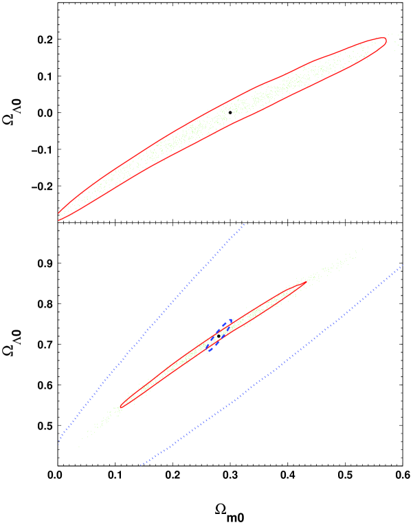
In Figure 1, we show the predicted AP likelihood contours in the ($\Omega_{m0},\Omega_{\Lambda 0}$)-plane for the 2QZ survey (solid lines), in the case $w=-1$, in a universe with arbitrary spatial curvature. The scattered points represent maximum likelihood best fit values for $\Omega_{m0}$ and $\Omega_{\Lambda 0}$. The assumed “true” values are ($\Omega_{m0}=0.3,\Omega_{\Lambda 0}=0$) and ($0.28,0.72$), for the top and bottom panels, respectively. In the top panel the displayed curve corresponds to the predicted $2\sigma$ likelihood contour. In the bottom panel the predicted $1\sigma$ contour (dashed line) for one year of SNAP data [25] is displayed, together with the predicted $1\sigma$ AP contour. For the SNAP contour, it is assumed that the intercept $\cal{M}$ is exactly known. To have some ground of comparison with current SNe Ia observations, in the same panel, we also plot (dotted lines) the Supernova Cosmology Project [2] $1\sigma$ contour (fit C). As expected, in both cases, the test recovers nicely the “true” values. We stress out that the test is very sensitive to the difference $\Omega_{m0}-\Omega_{\Lambda 0}$. From the bottom panel we note that the sensitivity to this difference is comparable to that expected from SNAP, of the order $\pm 0.01$. Comparatively, however, the test has a larger uncertainty in the determination of $\Omega_{m0}+\Omega_{\Lambda 0}$, of the order $\pm 0.17$. The degeneracy in $\Omega_{m0}+\Omega_{\Lambda 0}$ may be broken if we combine the estimated results for the AP test with, for instance, those from CMB anisotropy measurements, whose contour lines are orthogonal to those exhibited in the panels [26].

Figure 1: Simulated models at fixed $w=-1$ and corresponding predicted AP confidence contours (solid lines). In the top panel we show the predicted $2\sigma$ likelihood contour assuming a “true” model ($\Omega_{m0}=0.3,\Omega_{\Lambda 0}=0)$. In the bottom panel the predicted $1\sigma$ contour (dashed line) for one year of SNAP data [25] is displayed, together with the predicted $1\sigma$ AP contour. For both tests we consider $\Omega_{m0}=0.28$ and $\Omega_{\Lambda 0}=0.72$; also displayed is a $1\sigma$ confidence contour obtained by the Supernova Cosmology Project (dotted lines; [2]).

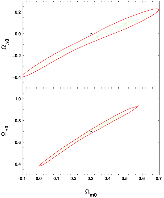
In order to estimate the consequences of neglecting the effect of linear peculiar velocities, in the top panel of Figure 2, we included them in the calculation of the $A_{i}$ values but neglected them in the computation of the maximum likelihood; in this panel, we assume $\Omega_{m0}=0.3$ and $\Omega_{\Lambda 0}=0$ as “true” values. Notice that the point with the “true” $\Omega_{m0}$ and $\Omega_{\Lambda 0}$ values is outside the $2\sigma$ contour. It is clear, therefore, the necessity of taking this effect in consideration when analyzing real data.

To illustrate that the AP test is in fact more sensitive to the mean amplitude of the bias rather than to its exact redshift dependence, we plot, in the bottom panel of Figure 2, the $2\sigma$ contour line, assuming as “true” values $\Omega_{m0}=0.3$ and $\Omega_{\Lambda 0}=0.7$. For this panel, the “true” $A_{i}$ values were generated assuming $b_{0}=1.45$ and $m=1.68$. However, for the simulations, we considered a constant bias ($m=0$), such that $b_{0,sim}:=\int_{z=z_{min}}^{z_{max}}F(z)b_{true}(z)dz=2.46$. We remark that the contour is slightly enlarged, mainly in the direction of the “ellipsis” major axis. However, the uncertainty in $\Omega_{m0}-\Omega_{\Lambda 0}$ is practically unaltered, confirming the strength of the test [27]. We did the same analysis assuming $\Omega_{m0}=1$ and $\Omega_{\Lambda 0}=0$ and obtained similar results.

Figure 2: Simulated models at fixed $w=-1$ and corresponding $2\sigma$ predicted AP confidence contour; in both panels, the “true” model is indicated by a solid dot. Top panel: The “true” model, $(0.3,0)$, takes into account the effect of peculiar velocities, but the simulated ones do not. Notice that the “true” model does not fall into the $2\sigma$ confidence region. Bottom panel: The “true” model, $(0.3,0.7)$, uses a redshift dependent bias function with $b_{0}=1.45$ and $m=1.68$, whereas the simulated ones use a constant bias equal to 2.46.

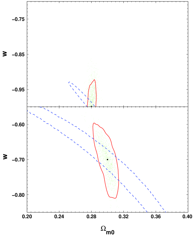
In Figure 3, we show the predicted AP likelihood contours in the $(\Omega_{m0},w)$-plane for the 2QZ survey (solid lines) for flat models ($\Omega_{k0}=0$). The “true” values are $(\Omega_{m0}=0.28,w=-1)$ and $(\Omega_{m0}=0.3,w=-0.7)$ for the top and bottom panels, respectively. In the top panel, we show, besides the AP contour, the predicted contour for one year of SNAP data (dashed line; [25]), both at $1\sigma$ level. For the SNAP contour, the intercept $\cal{M}$ is assumed to be exactly known. Notice that the contours are somewhat complementary and are similar in strength. In the bottom panel, we compare the predicted $95\%$ confidence contour of the AP test with the same confidence contour for the number count test as expected from the DEEP redshift survey (dashed line; [28]). Again the contours are complementary, but the uncertainties on $\Omega_{m0}$ and $w$ for the AP test are quite smaller.

Figure 3: Simulated flat models and corresponding predicted AP confidence contours (solid lines). The top panel is from a “true” model ($\Omega_{m0}=0.28$, $w=-1$), and displays the predicted confidence contours for the AP test and the SNAP mission (dashed line; [25]), both at $1\sigma$ level. The bottom panel is from a “true” model ($\Omega_{m0}=0.3$, $w=-0.7$), and displays the predicted confidence contours for the AP test and the DEEP survey (dashed line; [28]), both at the $95\%$ level.

In summary, we have shown that the Alcock-Paczyński test applied to the 2dF quasar survey (2QZ) is a potent tool for measuring cosmological parameters. We stress out that the test is especially sensitive to $\Omega_{m0}-\Omega_{\Lambda 0}$. We have established that the expected confidence contours are in general complementary to those obtained by other methods and we again emphasize the importance of combining them to constrain even more the parameter space. We have also revealed that, for flat models, the estimated constraints are similar in strength to those from SNAP with the advantage that the 2QZ survey will soon be completed.

Of course our analysis can be improved in several aspects. For instance, for the fiducial Einstein-de Sitter model, we have assumed that $\gamma$ and $r_{0}$ do not depend on redshift. In fact, observations [24] seem to support these assumptions, but further investigations are necessary. Since the test is very sensitive to $\Omega_{m0}-\Omega_{\Lambda 0}$, the effect of small-scale peculiar velocities should also be incorporated in future analyses in order to eliminate any potential source of systematic bias. At present, the quasar clustering bias is not completely well understood. Theoretical as well as observational progress in its determination will certainly improve the real capacity of the test. However, confirming previous investigations [27], we have found that the test is, in fact, more sensitive to the mean amplitude of the bias rather than to its exact redshift dependence. A more extensive detailed report of this work can be found in [29].

ACKNOWLEDGEMENTS

We would like to thank J. Silk for calling attention to the potential of the AP test and T. Kodama for suggestions regarding numerical issues. We also thank the Brazilian research agencies CNPq, FAPERJ and FUJB.

References

- [1] A. G. Riess et al., AJ 116, 1009 (1999).
- [2] S. Perlmutter et al., ApJ 517, 565 (1999).
- [3] Supernova Acceleration Probe: http://snap.lbl.gov/
- [4] P. de Bernardis et al., Nature 404, 955 (2000).
- [5] A. Balbi, et al., ApJ, 545, L1 (2000).
- [6] C. Pryke et al., astro-ph/0104490 (2001).
- [7] Microwave Anisotropy Probe: http://map.gsfc.nasa.gov/
- [8] Planck Surveyor: http://astro.estec.esa.nl/Planck/
- [9] Two-Degree Field Survey: http://www.aao.gov.au/2df/
- [10] Sloan Digital Sky Survey: http://www.sdss.org/
- [11] B. Ratra, and P. J. E. Peebles Phys. Rev. D, 37, 3406(1988).
- [12] J. A. Frieman, C. T. Hill, A. Stebbins, and I. Waga, Phys. Rev. Lett., 75, 2077 (1995).
- [13] R. R. Caldwell, R. Dave, and P. J. Steinhardt, Phys. Rev. Lett., 80, 1582 (1998).
- [14] P. Ferreira, and M. Joyce, Phys. Rev. D, 58, 023503 (1998).
- [15] C. Alcock, and B. Paczyński, Nature, 281, 358 (1979) [AP].
- [16] B. S. Ryden, ApJ, 452, 25 (1995).
- [17] W. E. Ballinger, J. A. Peacock, and A. F. Heavens, MNRAS, 282, 877 (1996).
- [18] T. Matsubara, and Y. Suto, ApJ, 470, L1 (1996).
- [19] L. Hui, A. Stebbins, and S. Burles, ApJ, 511, L5 (1999).
- [20] P. McDonald, and J. Miralda-Escudé, ApJ, 518, 24 (1999).
- [21] J. Kujat, A. M. Linn, R. J. Scherrer, and D. H. Weinberg, astro-ph/0112221 (2001)
- [22] P. A. Popowski, D. H. Weinberg, B. S. Ryden, and P. S. Osmer, ApJ, 498, 11 (1998) [PWRO].
- [23] S. Phillipps, MNRAS, 269, 1077 (1994).
- [24] S. M. Croom et al., MNRAS, 325, 483 (2001).
- [25] M. Goliath, R. Amanullah, P. Astier, A. Goobar, and R. Pain, Astron. Astrophys., 380, 6 (2001).
- [26] W. Hu, D. J. Eisenstein, M. Tegmark, and M. White, Phys. Rev. D, 59, 023512 (1999).
- [27] K. Yamamoto, and H. Nishioka, ApJ, 549, L15 (2001).
- [28] J. F. Newman, and M. Davis, ApJ, 534, L11 (2000).
- [29] M. O. Calvão, J. R. T. de Mello Neto, and I. Waga, Phys. Rev. Lett. (in press); astro-ph/0107029