The Star Formation Rate Intensity Distribution Function — Comparison of Observations with Hierarchical Galaxy Formation

Abstract

Recently, Lanzetta et al. (2002) have measured the distribution of star formation rate intensity in galaxies at various redshifts. This data set has a number of advantages relative to galaxy luminosity functions; the effect of surface-brightness dimming on the selection function is simpler to understand, and this data set also probes the size distribution of galactic disks. We predict this function using semi-analytic models of hierarchical galaxy formation in a $\Lambda$CDM cosmology. We show that the basic trends found in the data follow naturally from the redshift evolution of dark matter halos. The data are consistent with a constant efficiency of turning gas into stars in galaxies, with a best-fit value of $2\%$, where dust obscuration is neglected; equivalently, the data are consistent with a cosmic star formation rate which is constant to within a factor of two at all redshifts above two. However, the practical ability to use this kind of distribution to measure the total cosmic star formation rate is limited by the predicted shape of an approximate power law with a smoothly varying power, without a sharp break.

Key Words: galaxies: high-redshift, cosmology: theory, galaxies: formation

PACS: 98.80.-k, 98.62.Ai

1 Introduction

One of the major goals of the study of galaxy formation is to achieve an observational determination and a theoretical understanding of the cosmic star formation history. Previous measurements have generally found a factor of $\sim 4-10$ increase in the cosmic star formation rate (henceforth SFR) from redshift $z=0$ out to $z\sim 1$–2, with the cosmic SFR remaining roughly constant at higher redshifts out to $z\sim 4$, once approximate corrections are included for incompleteness or for the effect of dust extinction.

In general, estimates of the SFR apply locally-calibrated correlations between emission in particular lines or wavebands and the total SFR. The observational picture is based on a large number of observations in different wavebands. These include various ultraviolet/optical/near-infrared observations (e.g., Madau et al., 1996; Lilly et al., 1996; Madau, Pozzetti, & Dickinson, 1998; Treyer et al., 1998; Pettini et al., 1998; Cowie, Songaila & Barger, 1999; Glazebrook et al., 1999; Flores et al., 1999; Steidel et al., 1999; Hopkins, Connolly, & Szalay, 2000). At the shortest wavelengths, the extinction correction may be large (a factor of $\sim 5$ at the highest redshifts) and is still highly uncertain. At longer wavelengths, the star formation history has been reconstructed from submillimeter observations (Blain et al., 1999; Hughes et al., 1998) and radio observations (Cram et al., 1998); in this range of the spectrum, large uncertainties remain because of the insufficiency of current observational constraints on the spectral shape of the galaxies’ dust emission.

Hierarchical models have been used in many papers to match observations on star formation at $z\lesssim 4$ (e.g., Baugh et al., 1998; Kauffmann & Charlot, 1998; Somerville, Primack, & Faber, 2001). This comparison should become increasingly profitable for our physical understanding of galaxy formation as observations probe the galaxy population more completely at low redshift and also push towards high redshift.

Recently, Lanzetta et al. (2002) introduced a new data set, which takes advantage of the deepest images taken by the Hubble Space Telescope (HST), namely the Hubble Deep Field (HDF), and the Hubble Deep Field South (HDF-S) WFPC2 and NICMOS fields. These fields contain a fairly large number of galaxies, including a good fraction at high redshift. Combining a large variety of space- and ground-based optical and infrared images of these fields, Lanzetta et al. (2002) found photometric redshifts for $\sim 3000$ galaxies. They measured redshifts using a sequence of six spectral templates which account for different galaxy types. Their redshift technique has been checked with spectroscopic measurements at $z<6$, yielding a relative root-mean-square dispersion of 0.065 in $1+z$; however, the check applies mainly to $z=0$–1.2 and $z=2.2$-3.5, with only a small number of checks outside these redshift ranges (Yahata et al., 2000). Another limitation of the current data is that the fields are relatively small, and are not randomly selected. The HDF was chosen to be in a relatively empty field, while the HDF-S was chosen to be near a $z=2.2$ quasar. Thus, cosmic variance may be significant, although it should be greatly suppressed by the large redshift bins that are used in the analysis.

The data analysis of Lanzetta et al. (2002) presents several novelties compared to optical and infrared determinations of the galaxy luminosity function. Since most galaxies are well-resolved in the HST images, Lanzetta et al. (2002) divide each galaxy into individual pixels, and measure the SFR intensity $x$ in each pixel, in units of $M_{\odot}$ yr^-1 kpc^-2, where all quantities are proper. They then add up the proper areas of all pixels, within a given redshift range, with SFR intensity in the interval $x$ to $x+dx$. Dividing by the comoving volume in the redshift bin, and by $dx$, they obtain $h(x)$, the SFR intensity distribution function, expressed in units of proper kpc² per comoving Mpc³ per unit of $x$, i.e., kpc² Mpc${}^{-3}/(M_{\odot}$ yr^-1 kpc${}^{-2})$. Once $h(x)$ has been obtained, the total cosmic SFR per comoving volume is simply $\int x\,h(x)\,dx$.

Measuring the SFR in pixels offers a number of advantages compared to measuring the total SFR in a galaxy. First, as noted by Lanzetta et al. (2002), the total luminosity of a galaxy is in practice not very well defined, because the luminosity is integrated out to a radius where the surface brightness drops below the noise, and this radius depends strongly on redshift due to cosmological surface brightness dimming. In addition, the effect of surface brightness limits on the selection function is non-trivial in the case of galaxy luminosity functions; specifically, whether or not a galaxy is detected does not depend only on its luminosity, but also on its size and its orientation relative to the line of sight. On the other hand, since each pixel has a definite, known angular size, the selection function is simple, i.e., there is a minimum $x$ that can be detected within the pixel, as a function of redshift (and of position on the CCD). For this data set, the size distribution of galaxies does not enter as a nuisance in the data analysis, instead it enters as an important element of any theoretical model, an element which directly affects the predicted function $h(x)$.

Lanzetta et al. (2002) obtained the function $h(x)$ over a limited range of $x$ values in each of ten redshift bins. They then fit the curves to a broken power law model, allowing one of the parameters of the model to vary with redshift. The choice of a broken power law and of the allowed types of variation with redshift was motivated by the appearance of the data, not by any physical model of galaxy formation. Due to surface brightness dimming, at high redshift the observations can only detect the upper end of pixels, i.e., those with the highest SFR intensities. Indeed, at all redshifts $z>2$, most of the cosmic SFR occurs at $x$ values that are below the detection limit, and thus the total cosmic SFR is sensitive to an extrapolation which depends on the assumed shape of the function $h(x)$. In this paper, we confront the data with a semi-analytic model based on the theoretical understanding of hierarchical galaxy formation in a $\Lambda$CDM cosmology. We examine whether the model can explain the overall trends in the data, and we use the predicted, physically-motivated shape of $h(x)$ to carry out a measurement of the cosmic SFR.

The basic theoretical framework in which the matter content of the universe is dominated by CDM has recently received a major confirmation from measurements of the cosmic microwave background (Netterfield et al., 2002; Lee et al., 2002; Halverson et al., 2002). Based primarily on these measurements, in this paper we assume a $\Lambda$CDM cosmology with parameters $\Omega_{m}$ = 0.3, $\Omega_{\Lambda}$ = 0.7, $\Omega_{b}=0.05$, $\sigma_{8}=0.8$, $n=1$, and $h=0.7$, where $\Omega_{m}$, $\Omega_{\Lambda}$, and $\Omega_{b}$ are the total matter, vacuum, and baryon densities in units of the critical density, $\sigma_{8}$ is the root-mean-square amplitude of mass fluctuations in spheres of radius $8\ h^{-1}$ Mpc, and $n=1$ corresponds to a primordial scale-invariant power spectrum.

Throughout this paper we express results in physical units in $\Lambda$CDM. Note that Lanzetta et al. (2002) calculated results in an $\Omega_{m}=1$ cosmology, and expressed most quantities in units of $h=1$. We convert their measurements into our units and cosmology, using the redshift distribution of their galaxy sample. Note that $x$ depends on redshift but not on the cosmological matter content, since it is derived from observations of surface brightness. However, $h(x)$ and the cosmic SFR do change, through the change in both the proper area and the comoving volume corresponding to a given solid angle. Using $h=0.7$ reduces $h(x)$ by a factor of 1.4, and the conversion to $\Lambda$CDM causes an additional decline by a factor which equals 1.3 for the $z=0$–0.5 bin, and rises up to 1.8 for all $z>2$ bins.

In the following section we present the details of our theoretical model. Readers primarily interested in the comparison to the data may go directly to the summary of the basic setup in §3, the results in §4 and the conclusions in §5.

2 Theoretical Model

In this section we describe a model which allows us to predict the SFR intensity distribution function $h(x)$ in the context of hierarchical galaxy formation in $\Lambda$CDM. Briefly, we require the distribution of halo masses for halos which host galaxies, the SFR of each galaxy, and the size distribution of galactic disks.

We assume that the abundance of halos is given by the Press-Schechter model (Press & Schechter 1974; recent corrections to this model are insignificantly small for the current work). Galaxies form in halos in which gas can accumulate and cool. At high redshift, gas can cool efficiently in halos down to a virial temperature of $\sim 10^{4}$ K or a circular velocity of $V_{c}\sim 16.5\ {\rm km\ s}^{-1}$ with atomic cooling, which we assume to be the dominant cooling mechanism. Before reionization, the IGM is cold and neutral, and these cooling requirements set the minimum mass for halos which can host galaxies. During reionization, however, when a volume of the IGM is ionized by stars, the gas is heated to a temperature $T_{\rm IGM}\sim 1$–$2\times 10^{4}$ K. We adopt a standard temperature of $T_{\rm IGM}=1.5\times 10^{4}$ K, and then the linear Jeans mass corresponds to a virialized halo with a circular velocity of

$$V_{J}=82\left(\frac{T_{\rm IGM}}{1.5\times 10^{4}{\rm K}}\right)^{1/2}\ {\rm km\ s}^{-1}\ ,$$ (1)

where this value is essentially independent of redshift. Even halos well below the Jeans mass can pull in some gas once the dark matter collapses to the virial overdensity. For simplicity, we adopt a sharp cutoff associated with this suppression, at a circular velocity of $V_{c}=V_{J}/2$, based on the results of numerical simulations (Thoul & Weinberg, 1996; Quinn et al., 1996; Weinberg et al., 1997; Navarro & Steinmetz, 1997; Kitayama & Ikeuchi, 2000). However, this pressure suppression is not expected to cause an immediate suppression of the cosmic star formation rate, since even after fresh gas infall is halted the gas already in galaxies continues to produce stars, and mergers among already-formed gas disks also trigger star formation. Indeed, after reionization we assume that the minimum $V_{c}$ for hosting a galaxy rises with time only gradually, so that the total gas fraction in galaxies does not decline with time, as it physically must not [Some gas already in galaxies before reionization does photoevaporate at reionization, but this happens mostly in small halos which could not have cooled via atomic cooling (Barkana & Loeb, 1999)]. We assume that reionization occurs gradually, with H II regions fully engulfing the low density intergalactic medium at $z=6.5$, as suggested but not implied by recent observations (Becker et al., 2002; Djorgovski et al., 2002; Barkana, 2002). Note that while we include aspects of reionization in the model, this mostly affects the SFR at redshifts $z>4.5$, where the photometric redshifts may be less reliable; in this paper we focus on redshifts up to $z\sim 4$.

Once gas collects inside a halo and cools, it can collapse to high densities and form stars (and perhaps also a mini-quasar). The ability of stars to form is determined by gas accretion which, in a hierarchical model of structure formation, is driven by mergers of dark matter halos. Therefore, in order to determine the lifetime of a typical source, we first define the age of gas in a given halo using the average rate of mergers which built up the halo. Based on the extended Press-Schechter formalism (Lacey & Cole, 1993), for a halo of mass $M$ at redshift $z$, the fraction of the halo mass which by some higher redshift $z_{2}$ had already accumulated in halos with galaxies is

$$F_{M}(z,z_{2})={\rm Erfc}\left(\frac{1.69/D(z_{2})-1.69/D(z)}{\sqrt{2(S(M_{\rm min}(z_{2}))-S(M))}}\right)\ ,$$ (2)

where $D(z)$ is the linear growth factor at redshift $z$, $S(M)$ is the variance on mass scale $M$ (defined using the linearly-extrapolated power spectrum at $z=0$), and $M_{\rm min}(z_{2})$ is the minimum halo mass for hosting a galaxy at $z_{2}$ (as determined by the cutoff $V_{c}$ as was discussed above).

We estimate the total age of gas in the halo as the time since redshift $z_{2}$ where $F_{M}(z,z_{2})=0.2$, so that most ($80\%$) of the gas in the halo has fallen into galaxies only since then. Low-mass halos form out of gas which has recently cooled for the first time, while high-mass halos form out of gas which has already spent previous time inside small galaxies. We emphasize that the age we have defined here is not the formation age of the halo itself, but rather it is an estimate for the total period during which the gas which is currently in the halo has participated in star formation. However, the rate of gas infall is not constant, and even within the galaxy itself, the gas likely does not form stars at a uniform rate. Indeed, galaxies could go through repeated cycles of a star formation burst followed by feedback squelching, followed by another cycle of cooling, fragmentation and star formation. The details involve complex astrophysics, which are not understood even at low redshift, so we account for the general possibility of bursting sources by adding a parameter $\zeta\leq 1$, the duty cycle. When $\zeta<1$, compared to $\zeta=1$ there are fewer sources (by a factor of $\zeta$) but each has a larger SFR (by a factor of $1/\zeta$). Thus, $\zeta$ is a free parameter which does not change the total cosmic SFR. In addition, the cosmic SFR is proportional to the efficiency parameter $\eta$, which is the fraction of gas in each galaxy which turns into stars. In summary, the SFR of a galaxy in a halo of mass $M>M_{\rm min}(z)$ is

$${\rm SFR}=\frac{\Omega_{b}}{\Omega_{m}}\,\frac{\eta}{\zeta}\,\frac{M}{t_{\rm gas}}\ ,$$ (3)

where $t_{\rm gas}$ is the gas age as defined above.

A crucial element of the function $h(x)$ is its dependence on the size distribution of galactic disks. The formation of galactic disks within dark matter halos has been previously explored and compared to observed properties of disks at low redshift (Fall & Efstathiou, 1980; Dalcanton, Spergel, & Summers, 1997; Mo, Mao, & White, 1998). The observed distribution of disk sizes suggests that the specific angular momentum of the disk is similar to that of the halo. If they are assumed to indeed be equal, then for the simple model of an exponential disk in a singular isothermal sphere halo, the exponential scale radius of the disk is given by a fraction $\lambda/\sqrt{2}$ of the halo virial radius, where $\lambda$ is the dimensionless spin parameter of the halo (Mo, Mao, & White, 1998). The spin parameter distribution is approximately independent of halo mass, environment, and cosmological parameters, and approximately follows a lognormal distribution,

$$p(\lambda)d\lambda=\frac{1}{\sigma_{\lambda}\sqrt{2\pi}}\exp\left[-\frac{\ln^{2}(\lambda/\bar{\lambda})}{2\sigma_{\lambda}^{2}}\right]\frac{d\lambda}{\lambda}\ ,$$ (4)

with $\bar{\lambda}=0.05$ and $\sigma_{\lambda}=0.5$ following Mo, Mao, & White (1998), who determined these values based on the N-body simulations of Warren et al. (1992).

As a final element, we include a random orientation, i.e., a uniform distribution of the angle of each galactic disk relative to the line of sight to the observer. The distributions of both disk size and orientation must be integrated over in order to determine the observable function $h(x)$.

3 Basic Setup

Before discussing the results, we first summarize the essential properties of the data and the model, focusing on their primary advantages and disadvantages, some of which were discussed in the previous sections.

The advantages of the data set of Lanzetta et al. (2002) are:

1. A large number of galaxies ($\sim$3000), all imaged at high resolution with HST, and all with measured photometric redshifts.

2. Since most galaxies are well-resolved, the SFR can be measured within individual pixels rather than in entire galaxies. As a result, the effect of surface-brightness dimming on the selection function is simpler to understand than in the usual case of measuring the galaxy luminosity function.

3. The measured distribution, which focuses on the SFR intensity, is sensitive to the size distribution of galactic disks of a given luminosity, and thus the data allows a test of this additional aspect of theoretical models, unlike the galaxy luminosity function.

The disadvantages of the data set are:

1. The observed fields are very deep but relatively small in angular size, and they were not randomly selected. Thus, cosmic variance could be significant despite the large redshift bins that are used.

2. Since galaxies are pixelized, this introduces some smoothing relative to a comparison to a theoretical model, especially at high redshift where the number of pixels per galaxy is relatively small. Also, different photometric bands have different resolutions, so the spectrum of each galaxy is assumed to be fixed; if the actual spectrum varies among pixels in a given galaxy, then this affects the inferred SFR.

3. The photometric redshift measurements use six galactic spectral templates, while these templates may in reality evolve with redshift in unknown ways. However, this redshift technique has been checked with spectroscopic measurements, though mainly at $z=0$–1.2 and $z=2.2$-3.5 (Yahata et al., 2000).

The advantages of the theoretical model that we use are:

1. The model is based on the theoretical understanding of hierarchical galaxy formation within a $\Lambda$CDM cosmology, a cosmology which is strongly supported by recent observations.

2. The model assumes that galaxy formation is, on the whole, driven by the hierarchical merging of dark matter halos. Specifically, the timescale for star formation in a galaxy of a given mass and redshift is set by the infall history of the gas into halos.

3. Given the uncertainty, especially at high redshift, of the detailed properties of star formation and feedback, the model includes a reasonable flexibility with two free parameters, the efficiency of star formation, and a duty cycle ($\leq 1$) which allows for the possibility of episodic bursts of star formation.

4. The model includes the distribution of galaxy disk sizes which is expected theoretically, given the distribution of the angular momenta of dark matter halos. It also includes a random orientation of the disk relative to the line of sight.

5. The model accounts, in a simplified way, for the effect of reionization at redshift 6.5. This, however, mostly affects the star formation rate at redshifts $z>4.5$, where the photometric redshifts may be less reliable.

The disadvantages of the theoretical model are:

1. We do not include a distribution of possible merger histories for a halo of a given mass and redshift.

2. Our model focuses on disk galaxies, which should dominate star formation, especially at high redshift where most of the gas in a forming galaxy is falling in and forming stars for the first time. However, ellipticals and strongly irregular or disrupted disks are not correctly modeled in detail. Also, patchy star formation and extinction may make disks appear irregular in the rest-frame ultraviolet. Note, though, that the basic arguments for the star formation timescales and for the characteristic sizes of galaxies are very general, and should describe all galaxies sufficiently accurately for an initial comparison with observational data.

3. We do not model feedback processes in detail, only through the two free parameters. Also, we assume that the star formation efficiency and the duty cycle are constant, while more complicated models with additional free parameters are possible. E.g., we do not model cooling in detail, but increasing virial temperatures and decreasing densities should decrease the cooling efficiency at the lowest redshifts. Our approach is to first compare the data to a model which contains most of the relevant physics, in order to judge whether this type of data could, in the future, constrain even more detailed models.

4 Results

To begin the comparison, we first note that the points of Lanzetta et al. (2002) have a typical vertical $1-\sigma$ error of about a factor of 2 (up or down). It is difficult to estimate the additional systematic errors which arise from the just-noted limitations of the model and the data, but they are likely at least as large as the assigned error bars. In order to gauge the ability of the model to fit the data, we assume a minimum $1-\sigma$ error of a factor of 2 on each $h(x)$ bin, but we adopt the error bar of Lanzetta et al. (2002) on points where the error bar is larger than this.

Figure 1 compares the best-fit theoretical model to the data points of Lanzetta et al. (2002), converted into our units and cosmology (see the end of §1). Note that while the figure shows the smooth theoretical curves, in the fitting the theoretical predictions were binned into the same $x$-bins as the data. The best-fit parameter values and (formal) $1-\sigma$ errors are

$$\eta=2.3^{+0.4}_{-0.3}\%\ ,\ \ \ \ \zeta=17^{+7}_{-5}\%\ ,$$ (5)

with $2-\sigma$ ranges of $1.8\%<\eta<3.1\%$ and $9<\zeta<35\%$. The fit is acceptable, with a $\chi^{2}=59$ for 65 degrees of freedom (67 data points and 2 parameters). The fit is better over the redshift range with the most reliable data; fitting only the $z<4$ bins yields a $\chi^{2}=36$ for 55 degrees of freedom (with best-fit parameters $\eta=2.4\%$ and $\zeta=20\%$). Thus, the data are consistent with the theoretical model under the assumption of parameters $\eta$ and $\zeta$ which do not evolve with redshift. Note that a parameter $\zeta\sim 17\%$ is consistent with our assumption of regular disks, if the star formation bursts are triggered mostly by minor mergers which the disk may survive (e.g., Walker, Mihos, & Hernquist, 1996).

Hierarchical galaxy formation provides a natural explanation for the observed redshift evolution in the shape of $h(x)$. At high redshift, there is a shift towards higher values of SFR intensity, with $h(x)$ increasing at large $x$ and decreasing at small $x$. Galaxies at high redshift have lower typical masses than at low redshift, but the typical value of $x$ increases nonetheless because of two additional effects. First, high redshift disks are compact due to the increased mean density of the universe and the proportional increase in the typical density of virialized halos and of the disk galaxies forming within them. The second effect results from the vigorous star formation rates that are expected in high redshift galaxies despite their small masses. The increased rates of star formation are caused by the increased merger rate of dark matter halos. Since lower-mass halos are forming at high redshift, the power spectrum at the relevant mass scales is steeper, i.e., closer to the slope of $-3$ for which all mass scales would collapse together. Thus, at high redshift, when one mass scale collapses, a higher mass scale soon collapses as well, and this corresponds to a vigorous merger rate [For a further discussion of the redshift evolution of the size and surface brightness of galactic disks, see Barkana & Loeb (2000)].

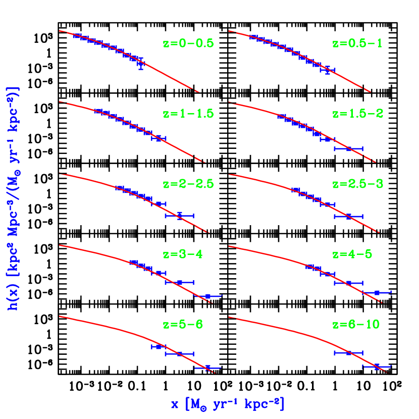
Figure 1: Comparison between our theoretical model and the data points of Lanzetta et al. (2002). Shown is the SFR intensity distribution function $h(x)$ versus SFR intensity $x$, for various redshift bins. Points with error bars are taken from Lanzetta et al. (2002), except that they are converted into our units and cosmology, and the error bars are slightly larger (see the text). Note that the horizontal brackets indicate bins, not error bars. Solid curves show the best-fit theoretical model (eq. 5).

Figure 2 illustrates how the shape of $h(x)$ is determined in the theoretical model. If all galactic disks are assumed to be face-on, and to also have a halo spin parameter equal to the average value ($\lambda=0.05$), then $h(x)$ is driven by the shape of the halo mass function and shows a steep drop-off at large values of $x$. If the spin-parameter distribution is included, $h(x)$ is smoother; the numerous galaxies in relatively low-mass halos contribute to high values of $x$ when $\lambda$ is small, and the break is smoothed from exponential to power law. Finally, including the distribution of disk orientations smoothes $h(x)$ further, and reduces the magnitude of the break in the power law. Figure 2 also shows that in the standard case with the full distributions, the shape of $h(x)$ depends only weakly on the precise value of $\sigma_{\lambda}$ in eq. (4).

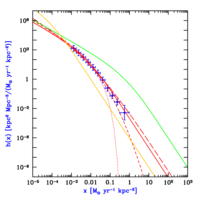
Figure 2: Theoretical models and data points in the $z=0.5-1$ redshift bin. Shown is the SFR intensity distribution function $h(x)$ versus SFR intensity $x$. Points with error bars are taken from Lanzetta et al. (2002) except for modifications (see the caption of Figure 1). The solid curve which goes through the data points shows the theoretical model with the parameters as in eq. (5). The other solid curves illustrate the effect of varying the parameters, i.e., multiplying $\eta$ by a factor of 100 (highest curve at $x=0.01$) or multiplying $\zeta$ by a factor of 100 (lowest curve at $x=0.01$). The three additional curves illustrate the effect on the shape of $h(x)$ of increasing $\sigma_{\lambda}$ in eq. (4) to unity (long-dashed curve), of assuming that all galactic disks are face-on (short-dashed curve), or of assuming that all galactic disks are face-on and have a halo spin parameter $\lambda=0.05$ (dotted curve).

Also shown in Figure 2 is the effect on $h(x)$ of changing the parameters $\eta$ and $\zeta$. The effect is simple in a log-log plot, e.g., multiplying $\eta$ by $10^{2}=100$ shifts the curve right by 2 and down by 2, while multiplying $\zeta$ by $100$ shifts the curve left by 2 and up by 4. More generally, given $h_{\eta,\zeta}(x)$, changing the parameters to $\eta^{\prime}$ and $\zeta^{\prime}$ yields the new function

$$h_{\eta^{\prime},\zeta^{\prime}}(x)=\left(\frac{\zeta^{\prime}}{\zeta}\right)^{2}\frac{\eta}{\eta^{\prime}}\ h_{\eta,\zeta}\left(\frac{\eta}{\eta^{\prime}}\frac{\zeta^{\prime}}{\zeta}x\right)\ .$$ (6)

As noted above, the total cosmic SFR is proportional to $\eta$ and independent of $\zeta$. The two parameters $\eta$ and $\zeta$ are really effective fitting parameters. For instance, the parameter $\eta$ includes the conversion between observed 1500Å flux and underlying SFR, which in turn includes assumptions about the stellar initial mass function. Also, any dust extinction reduces the fitted parameter $\eta$ compared to the actual star formation efficiency, and extinction could well be significant given the use of rest-frame ultraviolet wavelengths. The parameter $\zeta$, meanwhile, is exactly degenerate with the mean spin parameter; varying $\bar{\lambda}$ by a factor $\alpha$ affects $h(x)$ in the same way as would varying $\zeta$ by the factor $\alpha^{2}$. This latter degeneracy can in principle be lifted by combining measurements of $h(x)$ with other quantities such as the galaxy luminosity function.

Eq. (6) implies that instead of parameters $\eta$ and $\zeta$, we can choose two linear combinations (in a log-log plot) which correspond separately to shifting the $h(x)$ curve right or left, and shifting up or down. Thus, if $h(x)$ were an exact power law, there would be an exact degeneracy between the fitted values of $\eta$ and $\zeta$. Breaking this degeneracy requires a clear feature; however, the predicted shape of $h(x)$ is an approximate power law with only a smooth, gradual break. While the power law breaks more rapidly at high redshift, the $h(x)$ curve is observed over only a very limited range of $x$ values at high redshift, and thus the near-degeneracy remains. This degeneracy is clear in Figure 3, which shows two-parameter confidence limits for $\eta$ and $\zeta$. Indeed, the contours are elongated ellipses, and this limits our ability to separately measure each parameter. Note that the confidence regions for the fit to the entire data, and the separate fit to the $z=0.5-1$ bin (the bin with the largest number of data points), are consistent with each other, with the parameters constrained much more strongly in the single overall fit.

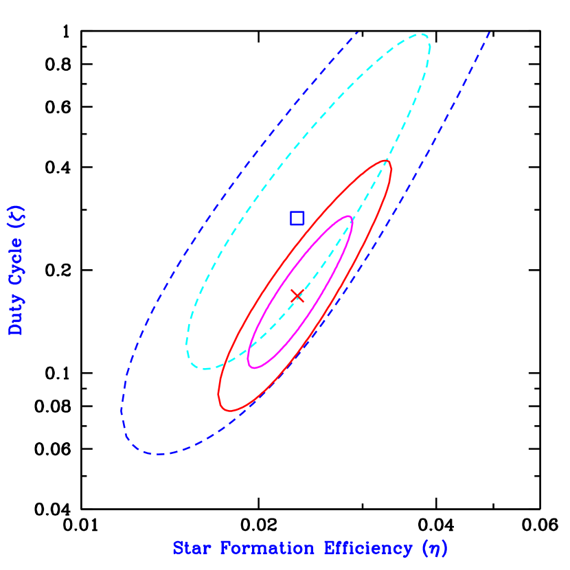
Figure 3: Two-parameter confidence regions, derived from the fitting of $h(x)$. Shown are constant $\chi^{2}$ curves in the $(\eta,\zeta)$ space. The $\times$ marks the best-fit point in the fit to the entire data set, and it is surrounded by solid curves which indicate $68\%$ and $95\%$ confidence limits, respectively. Similarly, the open square marks the best-fit point in the separate fit to the $z=0.5-1$ bin, and it is surrounded by dashed curves which indicate $68\%$ and $95\%$ confidence limits, respectively, for this case. Note that we cut off the figure at the top due to the constraint $\zeta\leq 1$.

Figure 4 shows the cosmic SFR versus redshift as derived from the fitting of $h(x)$. The results of fitting the theoretical model independently to each redshift bin are consistent, to about 1 $\sigma$, with the result of the simultaneous, overall fit to the data. Thus, there is no significant indication of an evolution in the parameters $\eta$ and $\zeta$. Our error bars on the independent fits in each bin are rather large, caused by the near-degeneracy between the parameters, as illustrated in Figure 3. Note that if we integrate over the cosmic star formation history, then the model with $\eta=2.3\%$ implies that the total density parameter in stars today is $\Omega_{*}\sim 0.15\%$. This is somewhat lower than the observed $z=0$ range of $0.19\%<\Omega_{*}<0.57\%$ (central value $0.35\%$; Fukugita, Hogan, & Peebles 1998), and suggests that extinction may be hiding a substantial fraction of the SFR (although the stellar initial mass function introduces additional uncertainties into this comparison).

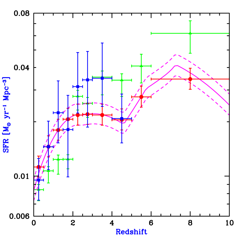
Figure 4: Cosmic SFR versus redshift, derived from the fitting of $h(x)$. The solid curve shows our best-fit theoretical model, with dashed curves showing the $1-\sigma$ range. Circles also show $h(x)$ from the theoretical model, but binned in redshift just like the data. Squares show the theoretical model binned in redshift, but these are results of independent fits to the $h(x)$ curves within each redshift bin (The two highest-redshift bins are not shown, since they contain too few data points to meaningfully constrain our two parameters). Triangles show the points from Figure 4 of Lanzetta et al. (2002) [specifically, their green circles, converted into our units and cosmology].

Figure 4 also shows one of the fits given by Lanzetta et al. (2002) to their data. Their results are generally consistent with our independent fits in each bin, although we do not find evidence for a large jump in the cosmic SFR at $z=2$. Their error bars are smaller than ours, but this is a result of their arbitrary decision to allow only a single parameter to vary in the fit within each redshift bin. Also, Lanzetta et al. (2002) give two other possible SFR histories from fits to the data; those fits are much higher than the one shown in Figure 4, by factors at $z=4$ of roughly 3 and 10, respectively, and those extrapolations from the data disagree strongly with our results, which are based on a physically-derived shape of $h(x)$. The shape of the cosmic SFR that we find, i.e., a sharp rise from $z=0$ to $z\sim 1$ followed by a flat segment out to $z\sim 4$, agrees with estimates based on extrapolations of the galaxy luminosity function (e.g., Steidel et al., 1999, and other references given in §1).

5 Summary

We have predicted the distribution of SFR intensity based on models of hierarchical galaxy formation. We have found that these models provide a natural explanation for the observed trend of the increase in the typical SFR intensity with redshift, an increase which occurs despite the decrease in the typical mass of galaxies. The observed data of Lanzetta et al. (2002) are consistent with a constant efficiency of turning gas into stars (best-fit $\eta=2.3\%$) and a constant duty cycle (best-fit $\zeta=17\%$). Thus, the data are consistent with the standard picture of the cosmic SFR rising from $z=0$ to $z=2$ and not increasing much further at $z>2$.

However, the $h(x)$ data are limited as a probe of star formation efficiency, since the broad spin-parameter distribution, along with the distribution of disk orientations, smoothes $h(x)$ into an approximate power law with only a gradual break. This break is difficult to measure, since only a limited range of $x$ values can be detected, especially at high redshift. Thus, two-parameter $\chi^{2}$ contours show a near-degeneracy between the two fitted parameters, and much more data would be required in order to fit even more detailed theoretical models of $h(x)$.

Luminosity functions of galaxies can be obtained for relatively large populations, using ground-based observations; also, if the total luminosity of each galaxy can be reliably measured, then this integrated quantity may allow a more robust comparison with theoretical models. However, data in the form of $h(x)$ do have a number of advantages. The effects of surface-brightness dimming and of the size distribution of galaxies can both be directly incorporated in the analysis, unlike the case of galaxy luminosity functions where both effects enter the selection function in ways that are difficult to model. In addition, other corrections may also be simpler; e.g., extinction may well depend directly on $x$, and not on the total luminosity of a galaxy, though high resolution images in many wavebands would be needed in order to determine the level of extinction separately in every pixel. Indeed, the upcoming Next Generation Space Telescope should produce a great leap forward for this type of data. It should probe a much wider range of $x$ values, with large numbers of galaxies detected over redshifts up to 10 and beyond. It should also provide high angular resolution over a wide range of optical and infrared wavelengths, which will likely allow it to overcome the limitations of current data.

References

- Barkana (2002) Barkana, R. 2002, New Astronomy, 7, 85
- Barkana & Loeb (1999) Barkana, R., & Loeb, A. 1999, ApJ, 523, 54
- Barkana & Loeb (2000) Barkana, R., & Loeb, A. 2000, ApJ, 531, 613
- Baugh et al. (1998) Baugh, C. M., Cole, S., Frenk, C. S., & Lacey, C. G. 1998, ApJ, 498, 504
- Becker et al. (2002) Becker, R. H., Fan, X., White, R. L., Strauss, M. A., & Narayanan, V. K. 2002, AJ, submitted (astro-ph/0108097)
- Blain et al. (1999) Blain, A. W., Smail, I., Ivison, R. J., & Kneib, J.-P., 1999, MNRAS, 302, 632
- Cowie, Songaila & Barger (1999) Cowie, L. L., Songaila, A., & Barger, A. J., 1999, AJ, 118, 603
- Cram et al. (1998) Cram, L. E., 1998, ApJL, 508, 85
- Dalcanton, Spergel, & Summers (1997) Dalcanton, J. J., Spergel, D. N., & Summers, F. J. 1997, ApJ, 482, 659
- Djorgovski et al. (2002) Djorgovski, S. G., Castro, S. M., Stern, D., & Mahabal A. 2002, ApJL, submitted (astro-ph/0108069)
- Fall & Efstathiou (1980) Fall, S. M., & Efstathiou, G. 1980, MNRAS, 193, 189
- Flores et al. (1999) Flores, H. et al. 1999, ApJ, 517, 148
- Fukugita, Hogan, & Peebles (1998) Fukugita, M., Hogan, C. J., & Peebles, P. J. E. 1998, ApJ, 503, 518
- Glazebrook et al. (1999) Glazebrook, K., Blake, C., Economou, F., Lilly, S., Colless, M. 1999, MNRAS, 306, 843
- Halverson et al. (2002) Halverson, N. W., Leitch, E. M., Pryke, C., Kovac, J., et al. 2002, ApJ, submitted (astro-ph/0104489)
- Hopkins, Connolly, & Szalay (2000) Hopkins, A. M., Connolly, A. J., & Szalay, A. S. 2000, AJ, 120, 2843
- Hughes et al. (1998) Hughes, D., et al., 1998, Nat, 394, 241
- Kauffmann & Charlot (1998) Kauffmann, G., & Charlot, S. 1998, MNRAS, 297, L23
- Kitayama & Ikeuchi (2000) Kitayama, T., & Ikeuchi, S. 2000, ApJ, 529, 615
- Lacey & Cole (1993) Lacey, C. G., & Cole, S. M. 1993, MNRAS, 262, 627
- Lanzetta et al. (2002) Lanzetta, K. M., Yahata, N., Pascarelle, S., Chen, H.-W., & Fernández-Soto, A. 2002, ApJ, in press (astro-ph/0111129)
- Lee et al. (2002) Lee, A. T., Ade, P., Balbi, A., Bock, J., et al. 2002, submitted (astro-ph/0104459)
- Lilly et al. (1996) Lilly, S. J., Le Fèvre, O., Hammer, F., & Crampton, D. 1996, ApJL, 460, 1lei
- Madau et al. (1996) Madau, P., Ferguson, H. C., Dickinson, M., Giavalisco, M., Steidel, C. C., & Fruchter, A. 1996, MNRAS, 283, 1388
- Madau, Pozzetti, & Dickinson (1998) Madau, P., Pozzetti, L., & Dickinson, M. 1998, ApJ, 498, 106
- Mo, Mao, & White (1998) Mo, H. J., Mao, S., & White, S. D. M. 1998, MNRAS, 295, 319
- Navarro & Steinmetz (1997) Navarro, J. F., & Steinmetz, M. 1997, ApJ, 478, 13
- Netterfield et al. (2002) Netterfield, C. B., Ade, P. A. R., Bock, J. J., Bond, J. R., et al. 2002, ApJ, submitted (astro-ph/0104460)
- Pettini et al. (1998) Pettini, M., Kellogg, M., Steidel, C. C., Dickinson, M., Adelberger, K. L., & Giavalisco, M. 1998, ApJ, 508, 539
- Press & Schechter (1974) Press, W. H., & Schechter, P. 1974, ApJ, 187, 425
- Quinn et al. (1996) Quinn, T., Katz, N., & Efstathiou, G. 1996, MNRAS 278, L49
- Somerville, Primack, & Faber (2001) Somerville, R. S., Primack, J. R., & Faber, S. M. 2001, MNRAS, 320, 504
- Steidel et al. (1999) Steidel, C. C., Adelberger, K. L., Giavalisco, M., Dickinson, M., & Pettini, M. 1999, ApJ, 519, 1
- Thoul & Weinberg (1996) Thoul, A. A., & Weinberg, D. H. 1996, ApJ, 465, 608
- Treyer et al. (1998) Treyer, M. A., Ellis, R. S., Milliard, B., Donas, J., & Bridges, T. J., 1998, MNRAS, 300, 303
- Walker, Mihos, & Hernquist (1996) Walker, I. R., Mihos, J. C., & Hernquist, L. 1996, ApJ, 460, 121
- Warren et al. (1992) Warren, M. S., Quinn, P. J., Salmon, J. K., & Zurek, W. H. 1992, ApJ, 399, 405
- Weinberg et al. (1997) Weinberg, D. H., Hernquist, L., & Katz, N. 1997, ApJ, 477, 8
- Yahata et al. (2000) Yahata, N., Lanzetta, K. M., Chen, H.-W., Fernández-Soto, A., Pascarelle, S., & Yahil, A. 2000, ApJ, 538, 493