ISOCAM observations of Galactic Globular Clusters:
mass loss along the Red Giant Branch.

Abstract

Deep images in the 10 $\mu$m spectral region have been obtained for five massive Galactic globular clusters, NGC 104 (=47 Tuc), NGC 362, NGC 5139 (=$\omega$ Cen), NGC 6388, NGC 7078 (=M15) and NGC 6715 (=M54) in the Sagittarius Dwarf Spheroidal using ISOCAM in 1997. A significant sample of bright giants have an ISOCAM counterpart but only $<$ 20% of these have a strong mid-IR excess indicative of dusty circumstellar envelopes. From a combined physical and statistical analysis we derive mass loss rates and frequency. We find that i) significant mass loss occurs only at the very end of the Red Giant Branch evolutionary stage and is episodic, ii)  the modulation timescales must be greater than a few decades and less than a million years, and iii) mass loss occurrence does not show a crucial dependence on the cluster metallicity.

1 Introduction

A complete, quantitative understanding of the physics of mass loss processes and the precise knowledge of the gas and dust content in Galactic globular clusters is crucial in the study of Population II stellar systems and their impact on the Galaxy evolution. It also has major astrophysical implications on related problems such as the ultraviolet excess found in elliptical galaxies (Greggio & Renzini 1990; Dorman et al. 1995) and the interaction between the intracluster medium and the hot halo gas (cf. e.g. Faulkner & Smith, 1991).

Indirect evidence for mass loss in Population II stars includes the observed morphology of the horizontal branch (HB) in the cluster color–magnitude diagrams, the pulsational properties of the RR Lyrae stars, and the absence of asymptotic giant branch (AGB) stars brighter than the red giant branch (RGB) tip (Rood 1973, Fusi Pecci & Renzini 1975; 1976, Renzini 1977, Fusi Pecci et al. 1993, D’Cruz et al. 1996). The expected mass loss is about $0.2\,M_{\odot}$ along the RGB and about $0.1\,M_{\odot}$ along the AGB (e.g. Fusi Pecci & Renzini 1976). As a consequence of such mass loss processes, dust and gas should be present in the intracluster medium, as diffuse clouds (cf. e.g. Angeletti et al. 1982) or concentrated in circumstellar envelopes. If no cleaning mechanism is at work between two Galactic plane crossings, a few tens solar masses of intracluster matter should be accumulated in the central regions of the most massive clusters (i.e. those with large central escape velocity).

Early searches (see Roberts 1988, Smith et al. 1990 and references therein) for this intracluster gas (HI, HII, CO) and more recently detection of ionized gas in 47 Tuc (Freire et al. 2001), yielded upper limits or marginal detections well below 1 $M_{\odot}$.

Mid–IR excesses and scattered polarized light have also been observed in the central region of massive globular clusters (Frogel & Elias, 1988; Gillet et al. 1988; Forte & Mendez 1989; Minniti et al., 1992; Origlia, Ferraro & Fusi Pecci 1995, Origlia et al. 1997b). They are mainly associated with long period variables evolving along the AGB. These preliminary results seem to indicate that in globular clusters even the brightest IR point sources are fainter than 1 Jy in the 10 $\mu$m spectral region and most of the emission comes from warm circumstellar dust with a minor photospheric contribution. Any diffuse component is much fainter than 10 mJy$\,{\rm arcsec^{-2}}$.

Other evidence of dust in the intracluster medium of globular clusters comes from the presence of IRAS sources (Lynch & Rossano 1990, Knapp & Gunn 1995, Origlia et al. 1996) in their central regions and from more recent surveys using ISOPHOT (Hopwood et al. 1999) and ground based sub-millimeter antennas (cf. e.g. Origlia et al. 1997a, Penny, Evans & Odenkirchen 1997, Hopwood et al. 1998).

However, all these studies show that globular clusters are deficient in diffuse intracluster matter and that some mechanism(s) must be at work to remove the gas and dust which should have accumulated between each passage through the Galactic plane (cf. e.g. Faulkner & Smith, 1991).

Given this observational scenario the desirability of a deep mid-IR survey of the central regions of globular clusters in the continuum and in selected dusty features is obvious. Such a deep, spatially resolved photometric survey became possible with the spectrophotometric capabilities of ISOCAM on board of the Infrared Space Observatory (ISO, Kessler et al. 1996). ISOCAM (Cesarsky et al. 1996) provided relatively fine spatial resolution, large field coverage, and high sensitivity in the 10 and 20 $\mu$m spectral regions.

Ramdani & Jorissen (2001) performed a deep survey at 12 $\mu$m in the external regions of 47 Tuc at different distances from the cluster center, with the specific goal of studying the mass loss during the AGB evolutionary stage. They cross-correlated their ISOCAM survey with the DENIS survey and found dust excess only in two well known bright variables, confirming the strong link between stellar pulsation activity and mass loss modulation.

With the goal of studying the mass loss during the RGB evolutionary stage, a deep survey of the very central regions of six, massive globular clusters has been made using ISOCAM with two different filters in the 10 $\mu$m spectral region. Mid-IR observations have the advantage of sampling an outflowing gas fairly far from the star (typically, tens/few hundreds stellar radii). At 10 $\mu$m the sampled material typically left the star a few decades previously. Thus mass loss rates inferred from the mid-IR will smooth the mass loss rate over a few decades. For astrophysical purposes it is the longterm average mass loss which is important. Conceptually one could sample different distances and smoothing times by observing at different wavelengths, however at this time that is not practical. At longer wavelengths detectors lack the requisite sensitivity; at shorter wavelengths the photosphere dominates.

2 The data set

Five massive Galactic globular clusters, NGC 104 (=47 Tuc), NGC 362, NGC 5139 (=$\omega$ Cen), NGC 6388, NGC 7078 (=M15) and NGC 6715 (=M54) in the Sagittarius Dwarf Spheroidal were observed with ISOCAM between February and August 1997, (proposals ISO_GGCS and DUST_GGC, P.I.: F. Fusi Pecci). Each of the clusters has an IRAS point source in its core (Origlia, Ferraro & Fusi Pecci 1996). The 12 $\mu$m IRAS flux is 1.7 Jy in 47 Tuc and 1.2 Jy in NGC 6388 and ranges between 0.4–0.5 Jy in the others. 47 Tuc, NGC 6388, and NGC 5139 show extended IRAS emission at 12 $\mu$m as well, with typical sizes of 2–4′ and total flux densities between 3 and 11 Jy.

Beam-switching observations were performed using CAM03 and 6″$\,{\rm pixel^{-1}}$ scale in two filters, LW7[9.6] (8.3–10.9 $\mu$m, centered on a silicate dust feature) and LW10[12] (8.6–15.4 $\mu$m, the IRAS 12 $\mu$m band). The total integration time for each cluster was about 2500s and the field of view was about 3′$\times$3′. 47 Tuc was also observed a second time in four filters, LW6[7.7] (6.9–8.5 $\mu$m), LW7[9.6], LW8[11.3] (10.7-11.9 $\mu$m) and LW10[12], for a total integration time of about 6700s and a field coverage of about 5′$\times$3′.

Near-IR photometry of the clusters observed with ISOCAM was obtained at ESO, La Silla (Chile), using the ESO-MPI 2.2m telescope and the near IR camera IRAC-2 (Moorwood et al. 1992) equipped with a NICMOS-3 256$\times$256 array detector, during different runs between 1992 and 1994. The frames were taken through standard $J$ and $K$ broad band filters. The overall spatial coverage is about 4′$\times$4′ with a 0$\farcs$5 pixel. More details on the reduction procedure and the photometric calibration are given by Ferraro et al. (1994; 2000) and Montegriffo et al. (1995). $\omega$ Cen was also observed (May 1999) with the ESO-NTT telescope using SOFI, the near-IR imager/spectrometer equipped with a 1024$\times$1024 array detector. The images were acquired through the $J$ and $K_{s}$ filters using a 0$\farcs$3 pixel scale. The $K_{s}$ photometry has been converted into the standard $K$ system using the stars in common with the IRAC-2 survey, and the calibration of Origlia, Ferraro & Fusi Pecci (1995). Accurate Point Spread Function (PSF) fitting reductions of the stellar fields have been carried out using the ROMAFOT package (Buonanno et al. 1983).

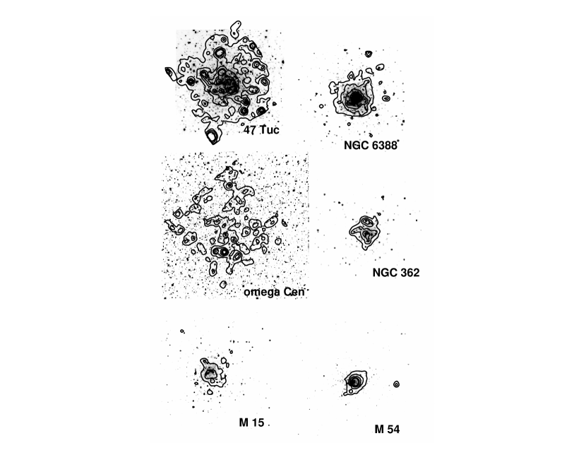
Figure 1: $K$ band images of the six clusters with the ISOCAM 12 $\mu$m emission contours at 2, 5, 10, 20 and 30 mJy superimposed. North is up, east is left. Each image field of view centered at the cluster center is about 4′$\times$4′. The bright, isolated 12 $\mu$m source on right side from the M54 center is associated with a Sagittarius field variable.

Fig. 1 shows the $K$ band images of the six clusters with the ISOCAM 12 $\mu$m contour plots superimposed. The latter were obtained using the background subtracted, mosaiced images (CMOS) generated by the ISOCAM auto-analysis pipeline (7.0 version of the off-line processing system).

3 Stellar Point Sources

The ISOCAM point source catalogs were also generated using the auto-analysis pipeline. For each beam–switching pointing the pipeline generates a calibrated flux image (CMAP) and the corresponding catalog of detected point sources. The point source searching and photometry was performed by maximum-likelihood estimates and PSF fitting. The nominal flux uncertainty is $\leq 20$%.

For each filter configuration we cross-correlated the various ISOCAM point source catalogs from the different beam-switching pointings and generated a final catalog with average fluxes and positions. This procedure has also allowed us to remove spurious detections due to possible transient or memory effects. The fluxes were first color–corrected, according to a blackbody energy distribution in the range of temperatures between 3000 and 5000 K, typical of the globular cluster red giants. The applied color–correction factors for the LW6[7.7], LW7[9.6], LW8[11.3] and LW10[12] filters are 1.06, 1.01, 1.00 and 1.26, respectively.

In order to convert the observed fluxes into magnitudes, 86.5, 66.4, 43.6 and 28.3 Jy were adopted as zero–magnitude fluxes at the reference wavelengths of the LW6[7.7], LW7[9.6], LW8[11.3] and LW10[12] filters, respectively. These zero point values were obtained using the IRAS flux density calibration at 12 $\mu$m (cf. Beichman et al. 1985) and a 10,000 K blackbody to obtain the zero-magnitude fluxes at the other reference wavelengths.

The near-IR stellar counterpart of each ISOCAM point source was identified by roto-translating the ISOCAM coordinate system into the near-IR system and cross-correlating the two catalogs with an overall accuracy $\leq$2 arcsec. Given the large pixel size of the ISOCAM images, several stars are often associated to each mid-IR source on the basis of the spatial coordinates alone. The brightest one within a square box of 30″ $\times$ 30″ (5 $\times$ 5 ISOCAM pixels) was selected. In all cases the brightest star turns to be also the reddest in (J-K).

The near-IR $J$ and $K$ magnitudes were de-reddened and transformed into bolometric magnitudes using the reddening and distance moduli given in Table 1, and the bolometric corrections as a function of the de-reddened $(J-K)_{0}$ colors listed by Montegriffo et al. (1998). The distance moduli in Table 1 are those from Harris (1996) with a $+0.2$ mag correction, based on the new calibration by Ferraro et al. (1999).

The average accuracy of the relative photometry is $\leq 0.2$ mag in the mid-IR and $\leq 0.1$ mag in the near-IR. The uncertainty of the zero point calibrations for absolute photometry is somewhat larger, a conservative estimate being $\leq 0.5$ mag.

In the two closest clusters, 47 Tuc and $\omega$ Cen, the limiting bolometric magnitude is $M_{\rm bol}\leq-1.0$; in M15 and NGC 6388 (the most distant ones in our Galactic sample) the detection threshold is $M_{\rm bol}\leq-2.5$. Our statistical analysis is based on this second limit. M54 in the Sagittarius Dwarf Spheroidal is more distant and even the brightest stars are close to the detection limit of our ISOCAM survey. The number of stellar counterparts identified in each cluster is given in Table 2. The $K$ band stellar maps of the six clusters down to a bolometric magnitude $M_{\rm bol}=-2.5$ and their associated ISOCAM point sources are plotted in Fig. 2. The only known variables in this sample are V42 in $\omega$ Cen (a long period variable) and six other stars with small amplitude variability and unknown period present in the observed field of view of 47 Tuc (cf. Montegriffo et al. 1995 and reference therein).

Using the ISOCAM mosaiced images (CMOS, cf. Fig. 1) we also performed aperture photometry of the central core region of each cluster within an $\approx 1\farcm 5$ radius. We then compared these integrated flux densities with those obtained by summing the contributions of each ISOCAM point source over the same field of view and determined an upper limit to the percentage concentrated in circumstellar (CS) envelopes with identified stellar counterparts. Both the total fluxes and these percentages are given in Table 2. These percentages scale approximately with the geometrical dilution, and very similar values are also inferred using the $K$ band flux, which is fully dominated by the stellar photosphere. Such a behavior suggests that the 12 $\mu$m emission not associated with bright circumstellar envelopes is most likely due to the unresolved stellar background, although some contribution by diffuse warm dust heated by the cluster radiation field can be also possible.

4 Color excess and dust parameters

Suitable color–magnitude and color–color diagrams of the ISOCAM point sources were constructed in order to quantify the relative photospheric and dust excess contribution. Fig. 3 shows the $M_{\rm bol},~{}(J-K)_{0}$ and $M_{\rm bol},~{}(K-[12])_{0}$ color–magnitude diagrams. Fig. 4 shows the corresponding $(K-[12])_{0},~{}(K-[9.6])_{0}$ color–color diagram.

The $(J-K)_{0}$ color mainly traces the photospheric temperature, thus defining the RGB ridge line of each cluster (Ferraro et al. 2000). Possible circumstellar dust excess is best shown using a combination of near and mid-IR colors. Overall a good correlation between the $(K-[12])_{0}$ and $(K-[9.6])_{0}$ colors is found, indicating that both the broad band continuum filter LW10[12] and the narrow band filter LW7[9.6] centered on a silicate dust feature are good tracers of dust excess. However, since the broad LW10[12] filter is somewhat more sensitive in detecting mid-IR excess and taking into account the actual color scatter along the observed RGB, $(K-[12])_{0}\approx 0.65$ was adopted as a conservative, border value between pure photospheric emission and significant dust excess. Mass loss at a lower rate could be traced by bluer $(K-[12])_{0}$ colors as well, but the observed photometric scatter and the spatial resolution of our mid-IR survey is not adequate to further constrain mass loss in this regime.

20 out of the 52 ISOCAM sources detected in the upper 1.5 bolometric magnitudes of the RGB show direct evidence of mid-IR circumstellar dust excess: 2 variables (V8 and V26, cf. Montegriffo et al. 1995) and 5 normal giants in 47 Tuc, 6 in NGC 6388, 3 in NGC 362, 2 in M15, the only candidate cluster member in M54 and the long period variable V42 in $\omega$ Cen (also see Table 2). The de-reddened photometry of these sources with dust excess is reported in Table 3. From pure evolutionary timescale considerations (e.g., Renzini & Fusi Pecci 1988), 10% or less of bright giants are expected to be in the AGB phase. Since we observed the very central region of each cluster where most of the luminous giants should be located, we expect less than 5 AGB stars in our global sample, hence when lacking further information we neglect them since they have a minor impact on the overall statistics. One exception is V42 in $\omega$ Cen: this star well fits the Period-Luminosity relation of classical Mira variables (especially if our slightly larger distance modulus is adopted, cf. Feast, Whitelock & Menzies, 2001) and it should be more likely on the AGB evolutionary stage, so we do not consider it in our further statistical analysis on the mass loss along the RGB.

In NGC 6388 and in M15, the most distant clusters in our Galactic sample, also very centrally concentrated, both the total number of ISOCAM sources and the number of those with mid-IR excess must be regarded as lower limits, since stellar counterparts to the 12 $\mu$m emission cannot be identified in the very central core where the crowding is too severe given the ISOCAM spatial resolution.

Somewhat surprisingly, no significant mid-IR excess has been found around any giant star in the observed central region of $\omega$ Cen. However, this cluster is known to be anomalous in many respects, with a multi-population RGB (cf. Pancino et al. 2000). More crucially in the current context, while the cluster is large in absolute size, it is very low density, and our sample size is small. Taking advantage of the wide field photometry recently published by Pancino et al. (2000), it has been possible to estimate that only $<30$% of the brightest giants are located in the central region covered by our mid-IR survey, while in the other clusters we sample almost all of the brightest giants. In order to obtain a similar statistical significance as in the other clusters of our survey, a much larger mid-IR spatial mapping is definitely needed.

In order to estimate the dust parameters a simple model using an optically and geometrically thin shell at constant temperature and with a $\nu B_{\nu}$ grain emissivity (cf. e.g. Natta & Panagia 1976; Origlia, Ferraro & Fusi Pecci 1996; Origlia et al. 1997b) has been computed. Standard grain radius and density of 0.1 $\mu$m and 3 g cm^-3, respectively, are adopted.

The mid-IR fluxes of those sources showing dust excess have been re-calibrated according to this modeling, using an average dust temperature of 300 K. The applied color–correction factors for the LW6[7.7], LW7[9.6], LW8[11.3] and LW10[12] filters are 1.01, 1.01, 1.00 and 0.95, respectively. The fraction of flux due to the photospheric emission has been neglected since it is small and always within the photometric errors.

The dust temperature has been inferred from the $([9.6]-[12])$ color in all clusters, for homogeneity. Since 47 Tuc has been also observed in two additional narrow band filters (LW6[7.7] and LW8[11.3], cf. Sect. 2), the $([7.7]-[11.3])$ and $([7.7]-[9.6])$ colors can be also used to derive dust temperatures and to check the consistency with those derived from the $([9.6]-[12])$ color. Fig. 5 shows that only minor ($<$50 K) systematic differences exist between the three methods. The inferred values of $T_{\rm dust}$ are between $\approx 200$ and $\approx 600$ K and the dust equilibrium radii $R_{\rm dust}$ between 300 and 40 stellar radii, respectively. The corresponding dust masses range between a few 10^-9 and a few 10^-7 $M_{\odot}$.

Fig. 6 shows that for lower dust temperature there is a somewhat larger dust mass, while there is not any evident correlation between the latter and the stellar luminosity.
The amount of material available to make dust in RGB stars must be proportional to the cluster metallicity. Only with helium burning stages could stars produce their own dust raw material; this should reach the surface only on the luminous AGB if then. Indeed, Fig. 6 shows that a large amount of dust has been only detected in the most metal rich clusters of our sample (47 Tuc and NGC 6388) while the two metal poor stars of M15 have low dust content.

5 Circumstellar mass loss

Empirical mass loss rates can be derived from dust masses by assuming a gas-to-dust ratio and a typical timescale for the outflow.

Since more dust should be present in more metal rich objects one also expects that the gas-to-dust ratio increases when metallicity decreases (cf. e.g. van Loon 2000). Assuming a gas-to-dust mass ratio of 200 in 47 Tuc, the value for the other clusters is scaled accordingly to their metallicity:

$$\rho=M_{\rm gas}/M_{\rm dust}=200\times 10^{-({\rm[Fe/H]}+0.76)}$$ (1)

An empirical estimate of the epoch of dust ejection can be inferred from the dust equilibrium radius and assuming an outflow velocity:

$$\tau_{\rm outflow}=R_{\rm dust}/v_{\rm outflow}$$ (2)

The outflow velocity should depend on the stellar luminosity and the gas-to-dust ratio (cf. e.g. Habing, Tignon & Tielens 1994). Larger luminosity leads to a higher momentum flow by the photons, and thus the kinetic energy and velocity in the flow could be higher. For lower gas-to-dust ratio the number of grains per molecule of gas is larger, and could lead to a higher outflow velocity. Adopting the Habing et al. (1994) relation:

$$v_{\rm outflow}\propto L_{\star}^{0.3}~{}\rho^{-0.5}$$ (3)

The dependence of the outflow velocity on the mass loss rate rapidly weakens as the latter increases (Habing et al. 1994), and it has been neglected in our computations.

Empirical mass loss rates averaged over the time required by dust to reach its equilibrium radius have been inferred using the relation:

$$dM/dt=\rho~{}M_{\rm dust}/\tau_{\rm outflow}$$ (4)

In order to check the impact of our simplified modeling on the inferred mass loss rates, several simulations using the DUSTY code (Ivezić, Nenkova & Elitzur 1999) have been performed. A large grid of values for the overall optical depth at 12 $\mu$m, stellar temperatures, dust grain sizes, compositions and inner bound temperatures has been explored, using the analytic approximation to compute the density distribution for radiatively driven winds.

For homogeneity with our computations an average grain radius of 0.1 $\mu$m has been used, but very similar results (within 10%) are obtained with a standard grain size distribution between 0.005 and 0.25 $\mu$m. An average stellar temperature of 3500 K has been adopted. Temperature changes of $\pm 500$ K yield overall infrared excesses, mass loss rates and terminal outflow velocities which are only $\leq 50$%, $\leq 30$% and $\leq 10$% different, respectively. Lowering the inner boundary dust temperature from 1000 K (our reference value) to 500 K, gives a larger (but always within a factor of 2) variation in the inferred infrared excess, mass loss rates and outflow velocities. Varying the shell thickness from 10 to 10,000 times the shell inner radius produces negligible variations.

Fig. 7 shows comparisons between the observed infrared excesses, mass loss rates and outflow velocities inferred by our simplified modeling and some suitable DUSTY simulations, scaled to the stellar luminosity and gas to dust ratio of the giants in 47 Tuc. A good, simultaneous consistency (within a factor of two) between the empirical and simulated values have been obtained for an optically thin dust with $\tau\leq 0.05$ and by assuming an outflow velocity of 14 ${\rm km\,s^{-1}}$ for a stellar luminosity $L_{\star}=1000~{}L_{\odot}$ and $M_{\rm gas}/M_{\rm dust}=200$, at the 47 Tuc metallicity.

For the stars with mid-IR excess in our sample the epochs of dust ejection are typically decades and total mass loss rates between 10^-7 and 10^-6 $M_{\odot}\,{\rm yr^{-1}}$ (cf. Table 3). The systematic uncertainty of these estimates, mainly due to the various model assumptions, is a factor of about 3.

Fig. 8 shows that the inferred mass loss rates are almost independent of the amount of circumstellar dust and stellar luminosity. Also there is not any obvious trend with metallicity within the scatter. Nevertheless, it is worth noticing that while the stars in the intermediate and metal rich clusters span the whole range of measured mass loss values, the two metal poor stars of M15 have rather high rates, despite the relative low content of dust (cf. Fig. 6). This is not surprising since one expects that among the most metal poor objects only those with large mass loss rates can have detectable dust. The blue tail HB morphology of M15 also shows that some of its stars (if genuine post-RGB stars) have lost almost their entire envelope on the RGB.

These inferred mass loss rates are finally compared with different empirical laws by Reimers (1975a,b), Mullan (1978), Goldberg (1979), and Judge & Stencel (1991) in Fig. 9. The reference formulae are taken from Catelan (2000, cf. Appendix and Figure 10), who revised the original ones taking advantage of the most extensive data set made available by Judge & Stencel (1991) and more recent data on intermediate and low mass giants. Our rates are about one order of magnitude larger than those predicted by these relations and do not show any clear dependence on stellar parameters. However, as pointed out by Catelan (2000) these relations are calibrated on Population I giants of relatively low luminosity and extrapolation to the short-lived evolutionary phases near the tip of the RGB might be fraught with uncertainty. These lower mass loss rates could be indeed consistent with the lower color excess (if any) possibly measured in 47 Tuc and $\omega$ Cen at $M_{bol}\geq-2.5$ (cf. Fig. 3 and Sect. 4).

6 Discussion

Dust grains are very efficient in absorbing and scattering starlight and could contribute to driving or accelerating stellar winds. However, as widely discussed in the recent review by Willson (2000), pure stationary flow models seem inadequate to describe the mass loss phenomena since a strongly dust-driven wind in an oxygen-rich star requires large light-to-mass ratios ($L/M>10^{4}\,L_{\odot}/M_{\odot}$). Only the coolest and most luminous AGB stars with direct signatures of dusty winds possibly satisfy this criterion. If winds are dust driven, non-steady phenomena like pulsational effects must be invoked to drive or enhance a stellar wind and to promote dust formation. The role of pulsating atmospheres in AGB mass loss has been considered for many years both on theoretical and observational basis (cf. Willson 2000 and references therein).

For stars on the RGB basic mass loss mechanisms are still quite unknown (cf. e.g. Judge & Stencel 1991) and matter of debate. There is observational evidence of small-amplitude and short period variability among giants close to the RGB-tip (cf. e.g. Welty 1985; Edmonds & Gilliland 1996), consistent with some oscillation activity (low-overtone radial or nonradial pulsations). Cacciari & Freeman (1983) and Gratton, Pilachowski & Sneden (1984), observed H$\alpha$ emission lines in hundreds of giants in a large sample of globular clusters. They initially argued that the H$\alpha$ emission was direct evidence for mass loss. However, interpreting H$\alpha$ emission can be complicated (Dupree 1986). For example, Dupree et al. (1994) suggest from its time variability that H$\alpha$ emission is due to atmospheric shocks which might drive the mass loss. In either interpretation the presence of H$\alpha$ emission in RGB spectra would generally indicate ongoing mass loss.

In the star in which mass loss is best understood, the Sun, the mass loss mechanism is ultimately tied to the magnetic field generated by the convective zone (e.g., Dupree 1986). Since cluster RGB stars have convective zones they could well have magnetic fields. There are no direct measurements of such fields, and interpreting signatures of chromospheric activity which might arise from magnetic fields is quite complex (e.g., Ayres et al. 1997). There is some recent evidence for RGB starspots which would imply magnetic activity (Stefanik et al. 2002). Soker (2000) and García-Segura et al. (2001) argue that magnetic activity might play a role in AGB mass loss on the basis of planetary nebula morphology.

Some non-canonical deep mixing in the upper RGB has been also invoked to produce excess luminosities and enhancing the mass loss close to the RGB-tip (cf. e.g. Sweigart 1997; Cavallo & Nagar 2000, Weiss, Denissenkov & Charbonnel 2000), but a solid physical picture of the overall impact on the red giant evolution is still lacking.

Can our observations give further information on the RGB mass loss process?

According to our mid-IR survey, strong mass loss processes seem to occur only close to the RGB-tip, during the last few million years of the RGB lifetime at $M_{\rm bol}\leq-2.5$ (Fusi Pecci & Renzini 1975; Salaris & Cassisi 1997). Moreover, only a fraction of giants detected by ISOCAM show strong mid-IR excess. This is especially clear in Fig. 3. Except near the very RGB-tip, stars with mass loss are scattered pretty uniformly along the RGB along with stars with no mass loss. Further, there is no smooth variation with the stellar luminosity. This suggests episodic mass loss processes. We will refer to the fraction of the time that mass loss is “on” as $f_{\rm ON}$. The fraction of time that the mass loss is “off,” or has dropped below our detection threshold, is $f_{\rm OFF}$. Since of the 52 ISOCAM sources 20 show evidence for mass loss, a first global estimate is $f_{\rm ON}\approx 0.4$. Considering the small numbers, there is no evidence that $f_{\rm ON}$ for the individual clusters varies from this global value.

Things are not so simple. In principle, all the stars brighter than $M_{\rm bol}\leq-2.5$ in each cluster should have been detected. In practice, due to the broad ISOCAM PSF, some stars are missed. First, while there is sometimes more than one star within an ISOCAM point source PSF, we selected only the brightest. Second, in the dense cores of M15 & NGC 6388 it is not possible to associate the ISOCAM objects with any near-IR stellar counterpart. The number of lost stars basically depends on the crowding, and thus on both the cluster distance and density—the larger their values the larger the number of stars in each pixel field of view, other things being constant.

To estimate the number of missed stars, we have computed the expected number of giants brighter than $M_{\rm bol}\leq-2.5$ within the ISOCAM field of view in two ways. First we used a theoretical approach: the fraction of light within the ISOCAM beam, was computed using a King model and the Specific Evolutionary Flux by Renzini & Buzzoni (1986), assuming an average lifetime $\leq 6$ Myr at $M_{\rm bol}\leq-2.5$ (Fusi Pecci & Renzini 1975; Salaris & Cassisi 1997). As an alternative we counted the number of stars detected in our $J,~{}K$ survey within the same beam. The two methods provide similar results (within 20%). The numbers are given in Table 2. These values are significantly larger than the corresponding number of ISOCAM point sources detected in each cluster, as expected given the wide ISOCAM PSF.

How can the missed stars affect our estimate of $f_{\rm ON}$? The missed stars may or may not be losing mass. Only if they differ in some systematic way from the detected stars will they affect $f_{\rm ON}$. Since the brightest and reddest star was selected and since strong mass loss occurs only close to the tip of the RGB, the missed (fainter) stars may be less likely to have mass loss. A lower limit can be obtained by assuming that none of the missed stars has detectable mass loss. In that case for each cluster $f_{\rm ON}\geq$ (number of stars with dust excess)/(total number of stars) (cf. last line of Table 2).

In 47 Tuc and NGC 362, where crowding does not severely affect statistics, $f_{\rm ON}\geq$15%, while lower values have been inferred in M15 and NGC 6388 but in this cluster the very central core region was not sampled. In $\omega$ Cen 3–4 stars with dust excess should have been detected if $f_{\rm ON}\geq$15% as in 47 Tuc and NGC 362, but taking into account that only $<30$% of the brightest giants are sampled (see Sect. 3), the expected number of detections drops down to $\leq 1$, fully consistent with the inferred zero value. The result of M54 is not statistical significant, since it is too distant (see also Sect. 3).

Broad time limits can be placed on the episodic variations. At average rates between 10^-7 and 10^-6 $M_{\odot}\,{\rm yr^{-1}}$ (cf. Table 3) each major mass loss event should occur on time scales somewhat shorter than the evolutionary times (5–6 Myr on the upper RGB) and longer than the time it takes the outflowing gas to reach the radii where we observe the dust, i.e., decades, whatever be the actual mass loss mechanism (several bursting episodes with multiple shells or more continuous flows). In principle such a lower limit to the episodic variation timescale can be as short as an instantaneous event, possibly at much higher mass loss rates, but our observations do not allow to constrain timescales with such a temporal resolution.

The total mass lost is crudely

$$\Delta M\sim{\rm rate}\times\Delta t_{\rm ON}$$ (5)

where $\Delta t_{\rm ON}$ is the total time interval in which a star experiences mass loss (either through many short-living episodes or a more continuous flowing).

In order to account for a total mass loss of about $0.2\,M_{\odot}$ required by the models to explain the HB morphology, and by assuming an average ${\rm rate}\approx 3\times 10^{-7}M_{\odot}\,{\rm yr^{-1}}$, $\Delta t$ should be $\approx 7\times 10^{5}\,{\rm yr}$, well within the inferred limits and almost one order of magnitude smaller than the total evolutionary time on the upper RGB.

Another interesting result seen from Figs. 8, 9 is that there is not any clear dependence of mass loss on metallicity, although more data, in particular for the metal poor clusters, are needed to draw firm conclusions. Again this result is not unexpected. The earlier H$\alpha$ studies also suggested little metallicity dependence in mass loss rates and are consistent with $f_{\rm ON}\sim 0.5$. However our observed time scales are much longer than the day to day variation observed in H$\alpha$ emission. Both the time scale and $f_{\rm ON}$ could be consistent with RGB magnetic cycles. Further, studies of horizontal branch morphology (Catelan & de Freitas Pacheco 1993; Lee, Demarque & Zinn 1994) suggest at most a mild metallicity dependence on mass loss efficiency except possibly at the lowest metallicities. In a recent paper van Loon (2000) analyzing the mass loss rates of a sample of obscured AGB stars also finds very modest dependence on metallicity, but possibly for different reasons related to the pulsation activity (e.g. van Loon 2001).

The observed metallicity independence of mass loss coupled with the fact that mass loss for RGB stars can be far below the criterion for radiatively driven winds suggests that dust may not be related to the driving mechanism for RGB mass loss. Dust can simply be a tracer of the out flowing gas and not responsible for the outflow.

7 Conclusions

Our ISOCAM survey of the central region of six massive globular clusters provided mid-IR photometry for 78 sources with identified stellar counterparts. 52 sources are associated with bright giants close to the RGB-tip. Of these about 40% have strong mid-IR excess ascribed to the presence of dusty circumstellar envelopes. Correcting for stars not detected because of the low spatial resolution of ISOCAM, dusty envelopes are inferred around about 15% of the brightest giants ($M_{\rm bol}\leq-2.5$).

The inferred mass loss rates are in the range $10^{-7}<dM/dt<10^{-6}M_{\odot}\,{\rm yr^{-1}}$, assuming as reference values an outflow velocity of 14 ${\rm km\,s^{-1}}$ and a gas-to-dust mass ratio of 200 at the metallicity of 47 Tuc and for a stellar luminosity of 1000 $L_{\odot}$.

The major astrophysical implications are:

• The mass loss occurs very near the RGB-tip and is episodic.

• The mass loss episodes must last longer than a few decades and less than a million years.

• There is no indication for a strict metallicity dependence of the frequency of mass loss occurrence.

Table 1: Adopted parameters for the observed globular clusters.

Cluster	$\alpha$ (2000)	DEC (2000)	Xa	Ya	[Fe/H]	$d$ [kpc]	E(B-V)	(m-M)V
NGC104 (= 47Tuc)	00 24 05	–72 04 51	30	218	$-0.76$	4.5	0.04	13.41
NGC362	01 03 14	–70 50 54	229	240	$-1.16$	8.7	0.05	14.86
NGC5139 (= $\omega$Cen)	13 26 46	–47 28 37	453	508	$-1.57$	5.4	0.12	14.04
NGC6388	17 36 17	–44 44 06	-6	223	$-0.60$	12.0	0.38	16.57
NGC6715 (= M54)	18 55 03	–30 28 42	254	262	$-1.59$	27.9	0.15	17.69
NGC7078 (= M15)	21 29 58	+12 46 19	138	93	$-2.22$	10.9	0.09	15.47

Note. —

^a Coordinates in pixel units (cf. Sect. 2 and Fig. 2) of the cluster center.

Table 2: ISOCAM point sources in the observed globular clusters.

Cluster (NGC)	104	362	5139	6388	7078	6715
	47Tuc		$\omega$Cen		M15	M54
Stellar Counterparts at $M_{\rm bol}\leq-2.5$	27	5	6	9	4	1
Stellar Counterparts at $M_{\rm bol}\leq-1.0$	40	…	19	…	…	…
Integrated central flux (Jy)at 12 $\mu$m	4.5	0.6	1.43	1.70	0.5	0.6
% of central 12 $\mu$m flux in resolved stars	45	22	26	8	12	2
Non-variable stars with dust excess	5	3	0	6	2	1
Variable stars with dust excess	V8, V26	…	V42	…	…	…
Estimated total of stars at $M_{\rm bol}\leq-2.5$	40	20	20	90	40	70
% of stars with dust excess at $M_{\rm bol}\leq-2.5$	$\geq$18	$\geq$15	$>$0	$>7$	$>5$	$>1$

Table 3: Infrared photometry and mass loss rates for the ISOCAM point sources with dust excess.

Cluster	stara	Xb	Yb	$K_{0}$	$(J-K)_{0}$	$(K-12)_{0}$	$M_{bol}$	$T^{d}_{dust}$ [K]	$\dot{M}^{c}$ [$M_{\odot}~{}yr^{-1}$]
47 Tuc	#1	55	186	6.74	0.96	1.20	$-3.92$	402	$2.5\times 10^{-7}$
	#2	8	181	7.78	0.99	0.70	$-2.84$	343	$8.5\times 10^{-8}$
	#3	$-7$	223	7.34	1.00	0.76	$-3.26$	491	$1.0\times 10^{-7}$
	#4	99	141	7.74	1.00	1.39	$-2.86$	291	$2.1\times 10^{-7}$
	#5	$-131$	276	7.15	1.12	2.14	$-3.28$	234	$1.1\times 10^{-6}$
	V8	3	330	6.83	1.23	1.64	$-3.46$	312	$4.8\times 10^{-7}$
	V26	9	257	6.55	1.24	1.16	$-3.73$	343	$3.4\times 10^{-7}$
NGC 362	#1	277	248	8.94	0.96	1.75	$-3.12$	335	$4.4\times 10^{-7}$
	#2	232	232	8.73	0.99	1.11	$-3.29$	339	$2.8\times 10^{-7}$
	#3	224	156	8.80	1.25	0.99	$-2.87$	271	$3.6\times 10^{-7}$
$\omega$ Cen	V42	438	686	8.51	0.89	2.35	$-2.58$	347	$7.1\times 10^{-7}$
NGC 6388	#1	17	308	9.62	0.85	0.98	$-3.30$	291	$1.4\times 10^{-7}$
	#2	$-89$	345	9.34	0.98	0.76	$-3.39$	297	$1.4\times 10^{-7}$
	#3	$-47$	291	8.86	1.08	0.75	$-3.73$	281	$2.2\times 10^{-7}$
	#4	89	274	9.74	1.08	1.04	$-2.85$	335	$1.2\times 10^{-7}$
	#5	34	266	9.11	1.16	1.36	$-3.37$	209	$6.8\times 10^{-7}$
	#6	$-24$	164	9.06	1.25	0.90	$-3.31$	276	$2.3\times 10^{-7}$
M15	#1	105	177	10.47	0.63	1.97	$-2.67$	397	$3.3\times 10^{-7}$
	#2	150	60	9.89	0.66	1.14	$-3.18$	572	$4.3\times 10^{-7}$
M54	#1	222	156	11.17	0.71	2.30	$-3.81$	272	$1.1\times 10^{-6}$

Note. —

^a Arbitrary numbering.

^b Coordinates in pixel units (the scale is 0.5″$\,{\rm pixel^{-1}}$ for all clusters but $\omega$ Cen which has 0.3″$\,{\rm pixel^{-1}}$, cf. Sect. 2).

^c Dust temperature assuming a $\nu B_{\nu}$ dust emissivity model (cf. Sect. 4).

^d Mass loss rates, by assuming reference outflow velocity of 14 ${\rm km\,s^{-1}}$ and gas-to-dust mass ratio of 200 at the metallicity of 47 Tuc (cf. Sect. 4) and for a stellar luminosity of 1000 $L_{\odot}$.

Figure 2: $K$ band stellar maps of the six clusters down to a bolometric magnitude $M_{\rm bol}\leq-2.5$. The ISOCAM 12 $\mu$m point source counterparts are overplotted (solid circles). North is up, east is left. The X and Y coordinates are in pixel units (the scale is 0.5″$\,{\rm pixel^{-1}}$ for all clusters but $\omega$ Cen which has 0.3″$\,{\rm pixel^{-1}}$, cf. Sect. 2). Each map field of view centered around the cluster center is about 4′$\times$4′. The cross indicates the nominal cluster center (cf. Table 1).

Figure 3: $M_{\rm bol}$,$~{}(J-K)_{0}$ (left panel) and $M_{\rm bol}$,$~{}(K-[12])_{0}$ (right panel) de-reddened color–magnitude diagrams down to a bolometric magnitude $M_{\rm bol}$ $\leq-1.0$ of the ISOCAM point sources detected in the observed globular clusters (cf. Sect. 4). Sources with $(K-[12])_{0}\geq 0.65$ are classified as sources with significant dust excess and are marked with filled symbols. The horizontal, dashed line at $M_{\rm bol}=-2.5$ marks the photometric threshold in the most distant clusters. The vertical, dashed line in the right panel marks the border between where 12 $\mu$m emission is dominated by the stellar photosphere or by circumstellar dust. The position of the V42 long period variable of $\omega$ Cen is also marked.

Figure 4: De-reddened $(K-[12])_{0},~{}(K-[9.6])_{0}$ color–color diagram of the ISOCAM point sources detected in the observed globular clusters (cf. Sect. 4). Symbols as in Fig. 3. The dashed box indicates the region where the 12 $\mu$m emission is still dominated by the stellar photosphere. Although there is a good overall correlation between the $(K-[12])_{0}$ and $(K-[9.6])_{0}$ colors, as a conservative approach only those sources with $(K-[12])_{0}>0.65$ are classified as having dusty envelopes (we then exclude the star in NGC 6388 with strong $(K-[9.6])_{0}$ color excess and photospheric $(K-[12])_{0}$, cf. Sect. 4). The position of the V42 long period variable in $\omega$ Cen is also marked.

Figure 5: Dust temperatures from different mid–IR colors $([7.7]-[12])$, $([7.7]-[11.3])$ and $([7.7]-[9.6])$ of the ISOCAM point sources with significant circumstellar dust excess (cf. Sect. 4) detected in 47 Tuc, assuming a $\nu B_{\nu}$ dust emissivity model. Symbols as in Figs. 3,4.

Figure 6: Dust mass as a function of dust temperature (left panel) and stellar luminosity (right panel) for the giant stars with dust excess (cf. Sect. 4). The position of the V42 long period variable of $\omega$ Cen is also marked. Symbols as in Figs. 3,4.

Figure 7: $(K-12)_{0}$ infrared excesses (lower panel), mass loss rates (middle panel) and outflow velocities (top panel) for the 7 giants in 47 Tuc with dust excess. Symbols as in Figs. 3,4. The dashed lines refer to DUSTY simulations at different optical depths, using as reference parameters an average stellar temperature of 3500 K, a grain radius of 0.1 $\mu$m, an inner boundary dust temperature of 1000 K and a shell outer radius 1000 times the shell inner radius (cf. Sect. 5).

Figure 8: Total mass loss rates as a function of dust mass (left panel) and stellar luminosity (right panel) for the giant stars with dust excess (cf. Sect. 4), by assuming reference outflow velocity of 14 ${\rm km\,s^{-1}}$ and gas-to-dust mass ratio of 200 at the metallicity of 47 Tuc and for a stellar luminosity of 1000 $L_{\odot}$. The position of the V42 long period variable of $\omega$ Cen is also marked. Symbols as in Figs. 3,4.

Figure 9: Mass loss rates for the giant stars with dust excess (cf. Sect. 4), as a function of different stellar parameters. The position of the V42 long period variable of $\omega$ Cen is also marked. Symbols as in Figs. 3,4. Different empirical laws by Reimers (1975a,b), Mullan (1978), Goldberg (1979), and Judge & Stencel (1991), recently revised by Catelan (2000, cf. his Appendix and Figure 10), calibrated on Population I giants of relatively low luminosity, are shown for comparison.

References

- (1)
- (2) Angeletti, L., Blanco, A., Bussoletti, E., Capuzzo-Dolcetta, R., & Giannone, P. 1982, MNRAS, 199, 441
- (3)
- (4) Ayres, T. R., Brown, A., Harper, G. M., Bennett, P. D., Linsky, J. L., Carpenter, K. G., & Robinson, R. D. 1997, ApJ, 491, 876
- (5)
- (6) Beichman, C. A., Neugebauer, G., Habing, H. J., Clegg, P.E., & Chester, T. J. 1985, IRAS Catalogs and Atlases Explanatory Supplement, (Washington: U.S. GPO)
- (7)
- (8) Buonanno, R., Buscema, G., Corsi C. E., Ferraro, I., & Iannicola, G., 1983, A&A, 126, 278
- (9)
- (10) Cacciari, C., & Freeman, K. C. 1983, ApJ, 268, 185
- (11)
- (12) Catelan, M. 2000, ApJ, 531, 826
- (13)
- (14) Catelan, M., & de Freitas Pacheco, J. A. 1993, AJ, 106, 1858
- (15)
- (16) Cavallo, R. M., & Nagar, N. M. 2000, AJ, 120, 1364
- (17)
- (18) Cesarsky, C.J., Abergel, A., Agnese, P. et al. 1996, A&A, 315, L32
- (19)
- (20) D’Cruz, N. L., Dorman, B., Rood, R. T., & O’Connell, R. W. 1996, ApJ, 466, 359
- (21)
- (22) Dorman, B., O’Connell, R. W., & Rood, R. T. 1995, ApJ, 442, 105
- (23)
- (24) Dupree, A. K. 1986, ARA&A, 24, 377
- (25)
- (26) Dupree, A. K., Hartmann, L., Smith, G. H., Rodgers, A. W., Roberts, W. H., & Zucker, D. B. 1994, ApJ, 421, 542
- (27)
- (28) Edmonds, P. D., & Gilliland, R. L. 1996, ApJ, 464, 157
- (29)
- (30) Faulkner, D. J., & Smith, G. H. 1991, ApJ, 380, 441
- (31)
- (32) Feast, M., Whitelock, P., & Menzies, J. 2001, MNRAS, in press, astro-ph/0111108
- (33)
- (34) Ferraro, F. R., Fusi Pecci, F., Guarnieri, M. D., Moneti, A., Origlia, L., & Testa, V. 1994, MNRAS, 266, 829
- (35)
- (36) Ferraro F. R., Messineo, M., Fusi Pecci, F., De Palo, M. A., Straniero, O., Chieffi, A., & Limongi M. 1999, AJ, 118, 1738
- (37)
- (38) Freire, P. C., Kramer, M., Lyne, A. G., Camilo, F., Manchester, R. N., & D’Amico, N. 2001, ApJ, 557, 105
- (39)
- (40) García-Segura, G., López, J. A., & Franco, J. 2001, ApJ, 560, 928
- (41)
- (42) Ivezić, Z., Nenkova, M., & Elitzur, M., 1999, User Manual for DUSTY, University of Kentucky Internal Report
- (43)
- (44) Lee, Y-W., Demarque, P., and Zinn, R. J. 1994, ApJ, 423, 248
- (45)
- (46) Ferraro F. R., Montegriffo, P., Origlia, L., & Fusi Pecci, F., 2000, AJ, 119, 128
- (47)
- (48) Forte, J. C., & Mendez, M. 1989, ApJ, 345, 222
- (49)
- (50) Frogel, J. A., & Elias, J. H. 1988, ApJ, 324, 823
- (51)
- (52) Fusi Pecci, F., & Renzini, A. 1975, A&A, 39, 413
- (53)
- (54) Fusi Pecci, F., & Renzini, A. 1976, A&A, 46, 447
- (55)
- (56) Fusi Pecci, F., Ferraro, F. R., Bellazzini, M., Djorgovski, G. S., Piotto, G., & Buonanno, R. 1993, AJ, 106, 1145
- (57)
- (58) Gillet, F. C., deJong, T., Neugebauer, G., Rice, W. L., & Emerson, J. P., 1988, AJ, 96, 116
- (59)
- (60) Goldberg, L. 1979, QJRAS, 20, 361
- (61)
- (62) Gratton, R. G., Pilachowski, C. A., & Sneden, C. 1984, A&A, 132, 11
- (63)
- (64) Greggio, L., & Renzini, A. 1990, ApJ, 364, 35
- (65)
- (66) Judge, P.G., & Stencel, R. E. 1991, ApJ, 371, 357
- (67)
- (68) Habing, H. J., Tignon, J., & Tielens, G. G. M. 1994, A&A, 286, 523
- (69)
- (70) Harris, W. E. 1996, AJ, 112, 1487
- (71)
- (72) Hopwood, M.E. L., Evans, A., Penny, A., & Eyres, S. P. S. 1998, MNRAS, 301, 30
- (73)
- (74) Hopwood, M. E. L., Eyres, S. P. S., Evans, A., Penny, A., & Odenkirchen, M. 1999, A&A, 350, 49
- (75)
- (76) Knapp, G. R., & Gunn, J. E. 1995, ApJ, 448, 195
- (77)
- (78) Kessler M. F., Steinz, J. A., Anderegg, M. E. et al. 1996, A&A, 315, L27
- (79)
- (80) Lynch, D. K., & Rossano, G. S. 1990, AJ, 100, 719
- (81)
- (82) Minniti, D., Coyne, S. J., & Claria, J. J. 1992, AJ, 103, 871
- (83)
- (84) Montegriffo, P., Ferraro, F. R., Fusi Pecci, F., & Origlia, L. 1995, MNRAS, 276, 739
- (85)
- (86) Montegriffo, P., Ferraro, F. R., Origlia, L., & Fusi Pecci, F. 1998, MNRAS, 297, 872
- (87)
- (88) Moorwood, A. F. M et al. 1992, The Messenger, 69, 61
- (89)
- (90) Mullan, D. J. 1978, ApJ, 226, 151
- (91)
- (92) Natta, A., & Panagia, N. 1976, A&AS, 50, 191
- (93)
- (94) Origlia, L., Ferraro, F. R., & Fusi Pecci, F. 1995, MNRAS, 277, 1125
- (95)
- (96) Origlia, L., Ferraro, F. R., & Fusi Pecci, F. 1996, MNRAS, 280, 572
- (97)
- (98) Origlia, L., Gredel, R., Ferraro, F. R., & Fusi Pecci, F. 1997a MNRAS, 289, 948
- (99)
- (100) Origlia, L., Scaltriti F., Anderlucci E., Ferraro, F. R., & Fusi Pecci, F. 1997b MNRAS, 292, 753
- (101)
- (102) Pancino, E., Ferraro, F. R., Bellazzini, M., Piotto, G., & Zoccali, M. 2000, ApJ, 534, L83
- (103)
- (104) Penny, A., Evans, A., & Odenkirchen, M. 1997, A&A, 317, 694
- (105)
- (106) Ramdani, A., & Jorissen, A. 2001, A&A, 372, 85
- (107)
- (108) Renzini, A. 1977, in Advanced Stellar Evolution, eds. P. Buovieri, & A. Maeder, (Saas-Fee: Geneva Obs.), 149
- (109)
- (110) Renzini, A., & Buzzoni, A. 1986, in Spectral Evolution of Galaxies, eds. C. Chiosi, & A. Renzini, (Dordrecht: Reidel), 135
- (111)
- (112) Renzini, A., & Fusi Pecci, F. 1988, ARA&A, 26, 199
- (113)
- (114) Reimers D. 1975a, in Problems in Stellar Atmospheres and Envelopes, eds. B. Baschek, W. H. Kegel, & G. Traving (Berlin: Springer), 229
- (115)
- (116) Reimers D. 1975b, in Mem. Soc. R. Sci. Liège 6 Ser., 8, 369
- (117)
- (118) Roberts, M.S. 1988, IAU Symp. 126, J.E. Grindlay & A.G.D. Philip eds., 411
- (119)
- (120) Rood, R. T. 1973, ApJ, 184, 815
- (121)
- (122) Salaris, M., & Cassisi, S. 1997, MNRAS, 289, 406
- (123)
- (124) Smith, G.H., Wood, P.R., Faulkner, D.J, & Wright, A.E., 1990, ApJ, 353, 168
- (125)
- (126) Soker, N. 2000, ApJ, 540, 436
- (127)
- (128) Stefanik, R. P., Carney, B. W., Latham, D. W., Morse, J. A., & Laird, J. B. 2002, BAAS, in press
- (129)
- (130) Sweigart, A. V. 1997, ApJ, 474, L23
- (131)
- (132) van Loon, J. T. 2000, A&A, 354, 125
- (133)
- (134) van Loon, J. T. 2001, ASP Conf. Ser, in press, astro-ph/0110167
- (135)
- (136) Weiss, A., Denissenkov P. A., & Charbonnel, C. 2000, A&A, 356, 181
- (137)
- (138) Welty, D. E. 1985, AJ, 90, 2555
- (139)
- (140) Willson, L. A. 2000, ARA&A, 38, 573
- (141)