Maximum-likelihood estimation of the CMB power spectrum from interferometer observations

Abstract

A maximum-likelihood method is presented for estimating the power spectrum of anisotropies in the cosmic microwave background (CMB) from interferometer observations. The method calculates flat band-power estimates in separate bins in $\ell$-space, together with confidence intervals on the power in each bin. For multifrequency data, the power spectrum of the other foreground components may also be recovered. Advantage is taken of several characteristic properties of interferometer data, which together allow the fast calculation of the likelihood function. The method may be applied to single-field or mosaiced observations, and proper account can be taken of non-coplanar baselines. The method is illustrated by application to simulated data from the Very Small Array.

1 Introduction

Interferometers have proven themselves to be valuable tools in observing anisotropies in the cosmic microwave background (CMB). They are inherently insensitive to anisotropies in atmospheric emission on scales larger than the beam and to ground spillover, and the fact that they sample Fourier space directly make interferometers ideal instruments for measuring the CMB power spectrum.

A method for calculating the maximum-likelihood CMB power spectrum directly from the complex visibility data produced by an interferometer was first discussed by Hobson, Lasenby & Jones (1995) (hereafter HLJ95). The method was illustrated by assuming the CMB anisotropies to be described by a Gaussian autocorrelation function, but the technique is easily modified so that the CMB power spectrum is parameterised in terms of flat band-powers in separate bins in $\ell$-space. Indeed, the modified HLJ95 algorithm was used to calculate flat band-power estimates of the CMB power spectrum in two spectral bins at $\ell\approx 410$ and $\ell\approx 590$ (with bin-width $\Delta\ell\approx 90$) for the Cosmic Anisotropy Telescope (CAT), which is a 3-element interferometer (Scott et al. 1996; Baker et al. 1999)

Following the early success of the CAT, a new generation of CMB interferometers have been built, and have recently made high-sensitivity observations of the CMB. These experiments include the Very Small Array (VSA) (Jones 1997; Jones & Scott 1998), the Degree Angular Scale Interferometer (DASI) (Leitch et al. 2001; Halverson et al. 2001) and the Cosmic Background Imager (CBI) (Pearson et al. 2000; Padin et al. 2001). Although the detailed design of these experiments is different in each case, the basic principles underlying their operation are the same. In particular, these instruments have a larger number of antennas than the CAT (for example, the VSA has 14 horns) and more sensitive detectors. These specifications enable the accurate measurement of the CMB power spectrum over a wide range of angular scales. For example, the VSA in its ‘compact’ configuration (see section 6) measures the CMB power spectrum in 10 independent bins of width $\Delta\ell\approx 90$ from $\ell\approx 80-950$.

Some discussion of how to obtain flat band-power estimates of the CMB power spectrum from this new generation of interferometer experiments has been presented by White et al. (1999a) and White et al. (1999b), mainly in connection with the analysis of DASI data. Indeed, the techniques outlined by these authors have been applied to the analysis of DASI and CBI observations. In particular, the DASI experiment has recently produced an accurate determination of the CMB power spectrum in 9 spectral bins of width $\Delta\ell\approx 80$ in the range $\ell\approx 100-900$ (Halverson et al. 2001), whereas the CBI has measured flat band-power estimates of the CMB power spectrum in two spectral bins at $\ell\approx 600$ and $\ell\approx 1200$, with a spectral resolution of $\Delta\ell\approx 400$ (Padin et al. 2001).

The increase in both the amount of visibility data and the number of independent spectral bins means that the computational burden of performing a likelihood analysis of the new generation of interferometer experiments is considerable. It is therefore of interest to investigate fast methods of calculating the likelihood function for interferometer observations of the CMB. In this paper, we extend the discussion given by HJL95 and White et al. (1999a, 1999b) and present a complete description of a maximum-likelihood technique for calculating flat band-power estimates of the CMB power spectrum from interferometer data. Following HJL95, the technique allows for contributions to the visibilities from Galactic foreground emission, which can be separated out if multifrequency data are available. In terms of the computational algorithm, we also present some straightforward devices for speeding up the calculation of the likelihood function, which take advantage of certain useful properties of interferometer data. Given the facility of fast evaluation of the likelihood function, we then investigate the relative merits of obtaining the maximum-likelihood flat band-power estimates, and their corresponding confidence intervals, either by direct evaluation the likelihood distribution, or by using traditional numerical maximisation techniques.

Our formalism makes no special assumptions specific to a particular experiment, and so can be applied to data from any CMB interferometer, including observations of mosaiced fields, and proper account is taken of non-coplanar baselines. The method is illustrated by applying it to simulated data from the Very Small Array (VSA). The application of the technique to real VSA observations will be presented in a forthcoming paper. We note, in passing, that a maximum-entropy map-making method for interferometer observations, which can simultaneously deconvolve the interferometer beam and separate CMB and Galactic foreground emission, is discussed by Maisinger, Hobson & Lasenby (1997).

2 Interferometer observations

Let us consider how an interferometer performs an observation of the CMB. We begin by discussing the likely contribution to the visibility data due to emission from different physical components at microwave wavelengths.

2.1 Model of the microwave sky

The total sky intensity $I(\hat{\mn@boldsymbol{x}},\nu)$ at a frequency $\nu$ in a direction $\hat{\mn@boldsymbol{x}}$ will, in general, contain contributions from the CMB and several foreground components, such as Galactic free-free and synchrotron emission, as well as emission from extragalactic radio point sources. As we discuss in section 3.1, contamination by point source emission is usually addressed by making simultaneous high-resolution observations of the sources, which may then be used to subtract the point source contribution from the data. We will therefore assume that point emission has been subtracted in this way, so that the remaining contamination of the CMB signal is due to diffuse Galactic emission.

We may express the fluctuations in the sky intensity as a sum over those due to each of these diffuse components

$$\Delta I(\hat{\mn@boldsymbol{x}},\nu)=\sum_{p=1}^{N_{p}}\Delta I_{\rm p}(\hat{\mn@boldsymbol{x}},\nu),$$ (1)

where $N_{p}$ is the number of distinct physical components contributing to the total sky emission. For the CMB component, it is more usual to work in terms of equivalent thermodynamic temperature fluctuations $\Delta T_{\rm cmb}(\hat{\mn@boldsymbol{x}})$, which is related to the intensity fluctuations by

$$\Delta I_{\rm cmb}(\hat{\mn@boldsymbol{x}},\nu)\approx\left.{\partial B(\nu,T)\over\partial T}\right|_{T=T_{0}}\Delta T_{\rm cmb}(\hat{\mn@boldsymbol{x}}).$$

where $B(\nu,T)$ is the Planck function and $T_{0}=2.726$ K is the mean temperature of the CMB (Mather et al. 1994). The conversion factor can be approximated by

$$\left.{\partial B(\nu,T)\over\partial T}\right|_{T=T_{0}}\approx 24.8~{}\left(\frac{x^{2}}{\sinh x/2}\right)^{2}~{}\mbox{Jy sr${}^{-1}$ ($\mu$K)${}^{-1}$},$$

where $x=h\nu/kT_{0}\approx(\nu/56.8~{}\mbox{GHz})$. For simplicity we define the brightness temperature fluctuations for the foreground components in a similar way. Thus, for the $p$th physical component of emission, we define

$$\Delta T_{p}(\hat{\mn@boldsymbol{x}},\nu)=\frac{\Delta I_{p}(\hat{\mn@boldsymbol{x}},\nu)}{\partial B(\nu,T_{0})/\partial T}.$$

We note that, in general, the ‘temperature’ fluctuations of the foreground components will be frequency dependent, unlike those of the CMB.

Temperature fluctuations on the sky are usually described by an expansion in spherical harmonics, so for each component we have

$$\frac{\Delta T_{p}(\hat{\mn@boldsymbol{x}},\nu)}{T}=\sum_{\ell=0}^{\infty}\sum_{m=-\ell}^{\ell}a_{\ell m}^{(p)}(\nu)Y_{\ell m}(\hat{\mn@boldsymbol{x}}),$$

from which we define the ensemble-average power spectrum of the $p$th component at some reference frequency $\nu_{0}$ by

$$c^{(p)}_{\ell}(\nu_{0})=\langle|a^{(p)}_{\ell m}(\nu_{0})|^{2}\rangle.$$

Since the power spectrum of the CMB is usually quoted in terms of the power per unit logarithmic interval in $\ell$, it is also useful to define the quantities

$$d^{(p)}_{\ell}(\nu_{0})=\ell(\ell+1)c^{(p)}_{\ell}(\nu_{0}).$$

For observations of small patches of sky, however, the spherical harmonic expansion is awkward to apply, and it is more convenient to use Fourier analysis, so that

$$\frac{\Delta T_{p}(\hat{\mn@boldsymbol{x}},\nu)}{T}=\int a^{(p)}(\mn@boldsymbol{u},\nu)\exp(2\pi i\mn@boldsymbol{u}\cdot\hat{\mn@boldsymbol{x}})~{}{\rm d}^{2}\mn@boldsymbol{u},$$

where $a^{(p)}(\mn@boldsymbol{u},\nu)$ is the Fourier transform of the temperature fluctuations in the $p$th physical component at an observing frequency $\nu$. The reason for including the factor of $2\pi$ in the exponent will become clear shortly, when we consider how an interferometer observes the sky. The two-dimensional transform variable $\mn@boldsymbol{u}$ is measured in wavelengths, and for later convenience we use $\rho=|\mn@boldsymbol{u}|$ to denote radial distances from the origin in the Fourier domain. For small fields, $\rho$ is related to the multipole $\ell$ in the spherical harmonic expansion by $\rho\approx\ell/2\pi$; the exact relationship is $\rho=\frac{1}{2}\cot(\pi/\ell)$ (see, for example, Hobson & Magueijo 1996). Since Fourier transformation is a linear operation, we may simply sum over the Fourier modes for each component to obtain an expression analogous to (1) for the Fourier transform of the total sky fluctuations

$$a(\mn@boldsymbol{u},\nu)=\sum_{p=1}^{N_{p}}a^{(p)}(\mn@boldsymbol{u},\nu).$$

It is convenient to separate the dependence of the Fourier modes on frequency $\nu$ and on position in the Fourier domain $\mn@boldsymbol{u}$. We are thus assuming that the spectral index of any Galactic emission does is not spatially varying over the observed field. For the compact VSA, for example, the extent of a single field is $\sim 4.6$ degrees, and so this assumption is not too severe. For mosaiced observations (see section 2.3) of larger areas of sky, however, this assumption may be questionable. We describe the frequency variation of each component through the functions $f_{p}(\nu)$ $(p=1,2,\ldots,N_{p})$. In this paper, we take the reference frequency $\nu_{0}=30$ GHz and normalise the frequency dependencies so that $f_{p}(\nu_{0})=1$ for all physical components.

If the emission in each component is statistically isotropic over the observed field and no correlations exist between the components, then the Fourier modes have mean zero and their covariance properties are given by

$$\langle a^{(p)}(\mn@boldsymbol{u},\nu)[a^{(p^{\prime})}(\mn@boldsymbol{u}^{\prime},\nu^{\prime})]^{*}\rangle=$$

$$\qquad\qquad\qquad C^{(p)}(\rho,\nu_{0})f_{p}(\nu)f_{p^{\prime}}(\nu^{\prime})\delta_{pp^{\prime}}\delta(\mn@boldsymbol{u}-\mn@boldsymbol{u}^{\prime}),$$ (2)

where $\rho=|\mn@boldsymbol{u}|$ and $C^{(p)}(\rho,\nu_{0})$ is the ensemble-average power spectrum of the $p$th physical component at the reference frequency $\nu_{0}$. Since the sky is real, the Fourier modes also obey $[a^{(p)}(\mn@boldsymbol{u},\nu)]^{*}=a^{(p)}(-\mn@boldsymbol{u},\nu)$. We note that the assumption of rotational invariance means that the ensemble-average power spectrum for each component is azimuthally symmetric in the Fourier domain and hence a function of $\rho$. For $\ell\ga 60$, we make contact with the spherical harmonic expansion by making the approximation

$$C^{(p)}(\rho,\nu_{0})\approx\left.c^{(p)}_{\ell}(\nu_{0})\right|_{\ell=2\pi\rho},$$

which is accurate to within one per cent. If we define the quantity $D^{(p)}(\rho,\nu_{0})=\rho^{2}C^{(p)}(\rho,\nu_{0})$, then in a similar way we find

$$D^{(p)}(\rho,\nu_{0})\approx\frac{1}{(2\pi)^{2}}\left.d^{(p)}_{\ell}(\nu_{0})\right|_{\ell=2\pi\rho}.$$

2.2 Visibility data

Expressing the temperature fluctuations of each component in terms of the Fourier modes $a^{(p)}(\mn@boldsymbol{u},\nu)$ is particularly useful when discussing interferometer observations. Assuming a small field size, and ignoring instrumental noise for the moment, an interferometer measures samples from the complex visibility plane ${\cal S}(\mn@boldsymbol{u},\nu)$ arising from the sky signal. After converting to temperature units, this is given by

$${\cal S}(\mn@boldsymbol{u},\nu)=\int A(\mn@boldsymbol{x},\nu)\frac{\Delta T(\mn@boldsymbol{x},\nu)}{T}\exp(2\pi i\mn@boldsymbol{u}\cdot\mn@boldsymbol{x})~{}{\rm d}^{2}\mn@boldsymbol{x},$$ (3)

where $\mn@boldsymbol{x}$ is the position relative to the phase centre, $A(\mn@boldsymbol{x},\nu)$ is the (power) primary beam of the antennas at the observing frequency $\nu$ (normalised to unity at its peak), and $\mn@boldsymbol{u}$ is a baseline vector in units of wavelength. In the following discussion, we assume the primary beam of a single antenna is circular symmetric and so does not vary with parallactic angle.

From (3), we see that $S(\mn@boldsymbol{u},\nu)$ is the Fourier transform of the product of the sky temperature fluctuations and the primary beam, which is equivalent to the convolution of the underlying Fourier modes $a(\mn@boldsymbol{u},\nu)$ with the Fourier transform of the primary beam $\widetilde{A}(\mn@boldsymbol{u},\nu)$,

$${\cal S}(\mn@boldsymbol{u},\nu)=a(\mn@boldsymbol{u},\nu)\star\widetilde{A}(\mn@boldsymbol{u},\nu).$$ (4)

The positions in the $uv$-plane at which this function is sampled by the interferometer are determined by the physical positions of its antennas and the direction of the field on the sky. The samples $\mn@boldsymbol{u}_{j}$ lie on a series of curves (or $uv$-tracks), which we may denote by the function $\widetilde{B}(\mn@boldsymbol{u},\nu)$ that equals unity where the Fourier domain (or $uv$-plane) is sampled and equals zero elsewhere. The function $\widetilde{B}(\mn@boldsymbol{u},\nu)$ may be inverse Fourier transformed to give the synthesised beam $B(\mn@boldsymbol{x},\nu)$ of the interferometer at an observing frequency $\nu$. For a realistic interferometer, the sample values will also contain a contribution due to instrumental noise. Thus, at an observing frequency $\nu$, the $j$th baseline $\mn@boldsymbol{u}_{j}$ of an interferometer (measured in wavelengths) measures the complex visibility

$${\cal V}(\mn@boldsymbol{u}_{j},\nu)={\cal S}(\mn@boldsymbol{u}_{j},\nu)+{\cal N}(\mn@boldsymbol{u}_{j},\nu),$$

where ${\cal N}(\mn@boldsymbol{u}_{j},\nu)$ is the instrumental noise on the $j$th visibility.

The effects of the convolution of the underlying Fourier modes with the aperture function and subsequent sampling are illustrated in Fig. 1, for the case when only CMB emission is present (and neglecting instrumental noise).

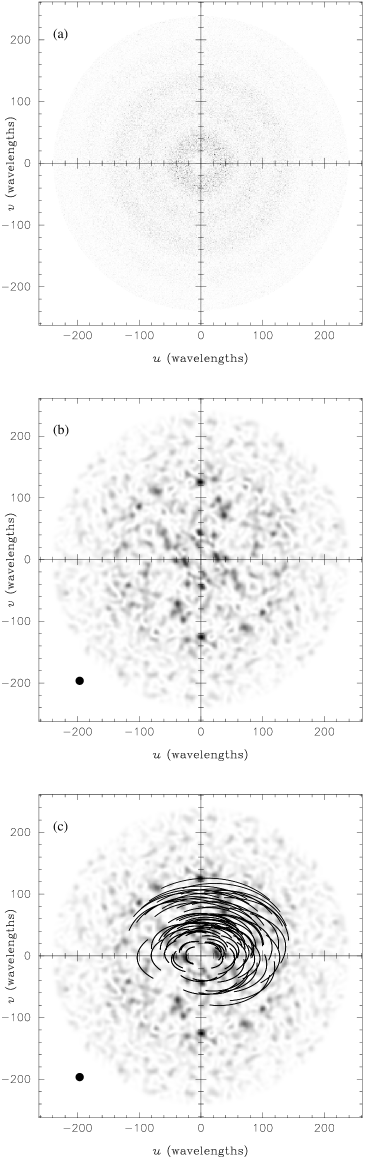
Figure 1: (a) A realisation of the two-dimensional CMB power spectrum for an inflationary CDM model (see text). (b) The same realisation as in (a), but convolved with the aperture function of our model interferometer, assuming a Gaussian primary beam of 4.6$\degr$ FWHM. (c) The $uv$-coverage for a simulated 5-h observation with a 14-element interferometer; each point corresponds to a sample with an integration time of 64-s.

In panel (a), we plot the modulus-squared of the underlying Fourier modes for a realisation of an inflationary CDM model with a Hubble parameter $H_{0}=$ 65 km s^-1 Mpc^-1 and a fractional baryon density $\Omega_{\rm b}=0.05$. The model is spatially flat with $\Omega_{\rm m}=0.3$ and $\Omega_{\Lambda}=0.7$, a primordial scalar spectral index $n=1$, and no tensor modes. The spectrum is normalised to COBE. We note the presence of acoustic ‘rings’ in this two-dimensional power spectrum. We also see that the different Fourier modes are uncorrelated. In panel (b), we plot the same realisation but after convolution with an aperture function corresponding to an interferometer with a Gaussian primary beam of 4.6$\degr$ FWHM. We see that the Fourier modes are no longer all independent, but appear correlated on lengths scales corresponding to the width of aperture function. The $1/e$ diameter of this function is plotted as the solid disc bottom left-hand corner of the figure. In panel (c) we overlay a typical 5-h $uv$-coverage for a compact VSA observation of a single field at a declination of 30$\degr$. This instrument consists of 14 antennas with physical separations lying between 20 cm and 1.50 m (see section 6). Each point corresponds to a sample with an integration time of 64 s.

2.3 Mosaicing

From (4), we see that in order to obtain a high resolution in Fourier space and thus in $\ell$-space, the Fourier transform of the primary beam needs to be narrow, implying large primary beams and small antennas. On the other hand, high sensitivity demands a large collecting area for each antenna. Clearly, some compromise has to be established between sensitivity and $\ell$-resolution, and the current generation of CMB interferometers differ in their respective priorities. However, the problem can be circumvented by a technique called mosaicing (Ekers & Rots 1979, Cornwell 1988, Cornwell et al. 1993, Holdaway 1999). Mosaicing consists of multiple observations of adjacent, overlapping fields on the sky. This increases the effective beam size of the telescope and thus the $\ell$-resolution.

Mosaicing exploits that a telescope samples along each baseline a whole superposition of visibilities. This is due to the finite extent of the the antenna aperture, which means that effectively all baselines corresponding to any two points on the two antennas that make up the baseline are sampled. Observations with different pointing centres probe different superpositions and can thus help to disentangle the individual contributions (Ekers & Rots 1979, Cornwell 1988).

Unfortunately, observations of overlapping fields also require that we take into account the correlations between the fields. In Appendix B we show that the effect of mosaicing may be be included by defining an effective primary beam $A_{\rm eff}(\mn@boldsymbol{x},\nu)$ that replaces $A(\mn@boldsymbol{x},\nu)$ in (3).

2.4 Non-coplanar baselines and $w$-corrections

For telescopes with a large primary beam $A(\mn@boldsymbol{x},\nu)$, the two-dimensional approximation (3) becomes inaccurate. Radiation incident away from the telescopes pointing centres suffers from phase errors if the $w$-components of the telescope baselines (i.e. the component in the direction of the source) do not vanish, or if the baselines are not coplanar. This is a geometric effect and is usually referred to as $w$-distortion or as non-coplanar baselines (see e.g. Cornwell & Perley 1993; Perley 1999).

In order to obtain a good resolution in Fourier space, the VSA has a comparatively large primary beam. While the antennas are all mounted on the same steerable table, they still track the source individually. This delay–tracking helps to identify foregrounds or other systematic errors by their different fringe rates. However, in the course of a longer observation, the projection of the source onto the telescope table changes and the array is effectively no longer coplanar.

This topic is discussed in detail in Appendix C, where we show that, similarly to mosaicing, again the effects of the non–coplanar baselines may be included by defining an appropriate effective primary beam $A_{\rm eff}(\mn@boldsymbol{x},\nu)$ that replaces $A(\mn@boldsymbol{x},\nu)$ in (3). Thus, the following discussion can be straightforwardly generalised to large fields.

3 Preliminary analysis

As discussed in HLJ95, before one can perform any meaningful statistical analysis, it is necessary to remove as many unwanted contributions as possible from the visibilities. It is also useful to compress the data sufficiently, such that the computational burden of the subsequent likelihood analysis is somewhat reduced.

3.1 Removal of bad data and point sources

Preliminary analysis of the time-ordered visibility data consists of the removal of periods of bad data due to poor weather conditions and system failures, and the subtraction of the contribution to the sky signal from identified discrete radio sources above some confusion limit. For example, O’Sullivan et al. (1995) discuss how this preliminary data analysis was carried out for CMB observations with the CAT interferometer, using the Ryle Telescope (Jones 1990) to perform the radio source subtraction. For VSA observations, the systematic removal of periods of bad data are performed in an analogous manner to that used for the CAT. The subtraction of point sources from VSA data again relies on Ryle Telescope observations to identify and determine the fluxes of all sources above some flux limit in the observed field. This process is also assisted by the use of two source-subtraction antennas situated adjacent to the main VSA instrument. The details of the point source identification and subtraction techniques used for VSA observations is discussed in Taylor (2000) and Taylor et al. (2001).

After periods of bad data and point source emission have been removed, the remaining non-cosmological contributions to the visibilities will then be from unsubtracted point sources below the flux limit of the observations, and from fluctuations in the Galactic free-free, synchrotron and dust emission. These foregrounds are usually identified by their spectral differences from the CMB, using multifrequency observations.

3.2 ‘Map’-making in the Fourier domain

For the new generation of CMB interferometers, the total number of visibilities at each frequency is very large. For example, the total number of 64-s samples in a typical 5-h observation with a 14-element interferometer is approximately 25,000, and any given field is observed for at least several days. It is therefore necessary to compress these data in some way, as discussed in HLJ95. This is analogous to the ‘map-making’ step in the analysis of single-dish CMB experiments, in which time-ordered data is binned into pixels on the sky (see, for example, Borrill 1999). For an interferometer, however, the visibilities at each observing frequency are binned into cells in the $uv$-plane.

Since we are not interested in making accurate CMB maps from the binned data, but are more concerned with estimating the CMB power spectrum correctly, the $uv$-plane is simply divided into equal-area square cells (or pixels) of side $\Delta u$, within each of which ${\cal S}(\mn@boldsymbol{u},\nu)$ is assumed to be constant. Clearly, only a small number $N_{c}$ of these cells will contain observed visibility samples. We assemble the (complex) values in each observed pixel into the (complex) vector $\mn@boldsymbol{s}$ of length $N_{c}$. We then calculate the maximum-likelihood solution for these $N_{c}$ values as follows.

Suppose that the total number of visibility samples at the observing frequency $\nu$ is $N_{v}$, and that the $j$th visibility is measured at a point $\mn@boldsymbol{u}_{j}$ in the $uv$-plane. Let us assemble these visibilities into the (complex) data vector v of length $N_{v}$, and also define the $N_{v}\times N_{c}$ pointing matrix with elements

$$M_{jk}=\left\{\begin{tabular}[]{ll}1&\mbox{if $\mn@boldsymbol{u}_{j}$ lies in the $k$th cell},\\ 0&\mbox{otherwise}.\end{tabular}\right.$$

In this way, we may write the data vector as

$$\textbf{{v}}=\textbf{{M}}\mn@boldsymbol{s}+\textbf{{n}},$$ (5)

where n is the (complex) noise vector of length $N_{v}$, whose $j$th element is simply ${\cal N}(\mn@boldsymbol{u}_{j},\nu)$. Assuming that the instrumental noise on the real and imaginary parts of the visibilities are independent and Gaussian, it is described by the complex multivariate Gaussian probability distribution (see Eaton 1983)

$$\Pr({\textbf{{n}}})=\frac{1}{\pi^{N_{v}}|{\textbf{{N}}}|}\exp(-{\textbf{{n}}}^{\dagger}{\textbf{{N}}}^{-1}{\textbf{{n}}}),$$ (6)

where ${\textbf{{N}}}=\langle{\textbf{{n}}n}^{\dagger}\rangle$ is the instrumental noise covariance matrix. Substituting (5) into (6), we find that the likelihood of obtaining the observed visibility data given a particular signal vector $\mn@boldsymbol{s}$ is given by

$$\Pr({\textbf{{v}}}|\mn@boldsymbol{s})=\frac{1}{\pi^{N_{v}}|{\textbf{{N}}}|}\exp[-({\textbf{{v}}}-{\textbf{{M}}}\mn@boldsymbol{s})^{\dagger}{\textbf{{N}}}^{-1}({\textbf{{v}}}-{\textbf{{M}}}\mn@boldsymbol{s})].$$

Maximising over $\mn@boldsymbol{s}$ then yields the maximum-likelihood solution, which we will denote by $\mn@boldsymbol{v}$ (instead of the more usual $\hat{\mn@boldsymbol{s}}$). We find that this vector of binned visibility data (of length $N_{c}$) is given in terms of the original visibility data vector v (of length $N_{v}$) by

$$\mn@boldsymbol{v}=({\textbf{{M}}}^{\rm t}{\textbf{{N}}}^{-1}{\textbf{{M}}})^{-1}{\textbf{{M}}}^{\rm t}{\textbf{{N}}}^{-1}\textbf{{v}}.$$ (7)

Moreover, if we substitute (5) back into (7), we find that the vector of binned visibilities can be written as

$$\mn@boldsymbol{v}=({\textbf{{M}}}^{\rm t}{\textbf{{N}}}^{-1}{\textbf{{M}}})^{-1}{\textbf{{M}}}^{\rm t}{\textbf{{N}}}^{-1}(\textbf{{M}}\mn@boldsymbol{s}+{\textbf{{n}}})=\mn@boldsymbol{s}+\mn@boldsymbol{n},$$

where

$$\mn@boldsymbol{n}=({\textbf{{M}}}^{\rm t}{\textbf{{N}}}^{-1}{\textbf{{M}}})^{-1}{\textbf{{M}}}^{\rm t}{\textbf{{N}}}^{-1}{\textbf{{n}}}.$$

This shows that the binned visibility data $\mn@boldsymbol{v}$ is the sum of the pixelised signal $\mn@boldsymbol{s}$ and some residual pixelised noise $\mn@boldsymbol{n}$ with covariance matrix

$$\mn@boldsymbol{N}=\langle\mn@boldsymbol{nn}^{\dagger}\rangle=({\textbf{{M}}}^{\rm t}{\textbf{{N}}}^{-1}{\textbf{{M}}})^{-1}.$$ (8)

It is instructive to consider the special case in which the original instrumental noise covariance matrix N is diagonal, so that the instrumental noise on each original visibility is uncorrelated. In fact, this is usually the case for interferometer data, and we may write ${\textbf{{N}}}=\mbox{diag}(\sigma_{1}^{2},\ldots,\sigma_{N_{v}}^{2})$, where $\sigma_{j}^{2}$ is the variance of the instrumental noise on the $j$th original visibility. In this case, it is straightforward to show that the maximum-likelihood solution (7) reduces to simple cell-averaging. Thus, the value $v_{k}$ of the binned visibility in the $k$th cell is given by

$$v_{k}=\frac{\sum_{j=1}^{m}{\cal V}_{j}/\sigma_{j}^{2}}{\sum_{j=1}^{m}1/\sigma_{j}^{2}},$$

where $m$ is the number of original visibilities lying in that cell. Similarly, from (8), we find that the residual pixelisation noise has the covariance matrix $\mn@boldsymbol{N}=\mbox{diag}(\epsilon_{1}^{2},\ldots,\epsilon_{N_{c}}^{2})$, where

$$\epsilon_{k}^{2}=\frac{1}{\sum_{j=1}^{m}1/\sigma_{j}^{2}}.$$

At each observing frequency $\nu$, it is the binned visibility vector $\mn@boldsymbol{v}$ and pixelised noise vector $\mn@boldsymbol{n}$ that constitute the basic data which are analysed in the estimation of the CMB power spectrum. It is usual to associate the $k$th binned visibility $v_{k}$ and noise $n_{k}$ with the the position $\mn@boldsymbol{u}_{k}$ that corresponds to the centre of the $k$th cell in the $uv$-plane. This is, however, not necessary. Indeed, one may preserve more information regarding the distribution of samples in the $uv$-plane by instead choosing $\mn@boldsymbol{u}_{k}$ to be the ‘centre-of-mass’ of the positions of the visibility samples within the $k$th cell.

It only remains to choose the size of the cells $\Delta u$ in the $uv$-plane. Since the speed with which the likelihood function can be calculated is strongly dependent on the number of binned visibility points that are analysed, we must make a compromise between how accurately the binned data represent the original visibilities, and the desire to use fewer data points in order to speed up the calculation. In fact, two natural limits exist for $\Delta u$.

A minimum size for the $uv$ cells is given by the requirement that each binned point on the grid represents an independent estimate of the underlying visibility. If the typical sample time per visibility is $\tau$ sec, then for samples at a distance from the $uv$-origin of $|\mn@boldsymbol{u}|$, time-smearing will correlate visibilities separated along a $uv$-track by less than approximately

$$\Delta u\approx 2\pi|\mn@boldsymbol{u}|\frac{\tau}{24\times 60\times 60}.$$

For $\tau=64$ sec and $uv$-coverage which extends out to $|\mn@boldsymbol{u}|\approx 200$ wavelengths, then $\Delta u\ga 1$ wavelengths.

A maximum size for the $uv$ cells is derived by considering the fact the measured visibilities are obtained by a convolution of the underlying Fourier modes with the interferometer aperture function. For example, the VSA in its compact configuration, this function is a Gaussian a FWHM of approximately 12 wavelength. Hence, as discussed by HLJ95, from the sampling theorem we require $\Delta u\la 6$ wavelengths. Nevertheless, finer binning is still useful since it provides better approximation for the position of the visibilities in the $uv$-plane. Thus, we find that the $uv$ cell size is reasonably well determined by our two limiting cases and for the simulations considered here we use $\Delta u=3$ wavelengths.

As an illustration, in Fig. 2 we plot the positions of the binned visibilities corresponding to the samples shown in Fig. 1(c). Each dot shows the position $\mn@boldsymbol{u}_{k}$ of the ‘centre-of-mass’ of each cell, with which the binned visibility $v_{k}$ is associated. In this case, the number of non-zero binned visibilities is approximately 2500. Provided the geometry of the interferometer is not varied, each period of observation of a given field will produce visibility samples lying in the same set of cells in the $uv$-plane. Thus, after binning the total number of complex data points at each observing frequency that are used to estimate the CMB power spectrum is about 2500.

Figure 2: An illustration of the positions of the binned visibilities resulting from the samples shown in Fig. 1(c) using a cell size $\Delta u=3$ wavelengths.

4 The visibilities covariance matrix

After binning, the data consist of the binned visibility data vector $\mn@boldsymbol{v}(\nu_{i})$ $(i=1,\ldots,N_{f})$ at each of the $N_{f}$ observing frequencies, together with the corresponding noise vector $\mn@boldsymbol{n}(\nu_{i})$ at each frequency. To keep our notation simple, we combine all the binned visibilities into the single data vector $\mn@boldsymbol{v}$, and all the noise vectors into a single vector $\mn@boldsymbol{n}$.

Let us assume that the $j$th binned visibility is measured at a point $\mn@boldsymbol{u}_{j}$ in the $uv$-plane and at an observing frequency $\nu_{j}$. From this point onwards, we shall denote the $j$th binned visibility by ${\cal V}_{j}$. Similarly, we shall denote the noise on the $j$th binned visibility by ${\cal N}_{j}$ and the contribution from the sky signal by ${\cal S}_{j}$. With a view to a practical implementation, it is easier to pursue the analysis in terms of the real and imaginary parts of each visibility, which we write as

$${\cal V}_{j}\equiv{\cal V}_{j}^{(R)}+i{\cal V}_{j}^{(I)}.$$

We may also divide the signal and noise contributions ${\cal S}$ and ${\cal N}$ into their real and imaginary parts in the same way. Thus, if the interferometer observation (including all observing frequencies) consists of total number $N_{t}$ of complex binned visibilities, we adopt the convention that the data vector $\mn@boldsymbol{v}$ is of length $N_{d}=2N_{t}$, consisting of first the real parts and then the imaginary parts of the visibilities, i.e.

$$v_{j}={\cal V}_{j}^{\rm(R)},\qquad v_{N_{t}+j}={\cal V}_{j}^{\rm(I)}.$$

It is also useful to write $\mn@boldsymbol{v}=\mn@boldsymbol{s}+\mn@boldsymbol{n}$, where the signal vector $\mn@boldsymbol{s}$ and noise vector $\mn@boldsymbol{n}$ are defined in a similar way.

Assuming there are no correlations between the contributions to visibilities from the sky signal and the instrumental noise, the covariance matrix of the interferometer data is given by

$$\mn@boldsymbol{C}=\langle\mn@boldsymbol{v}\mn@boldsymbol{v}^{\rm t}\rangle=\langle\mn@boldsymbol{s}\mn@boldsymbol{s}^{\rm t}\rangle+\langle\mn@boldsymbol{n}\mn@boldsymbol{n}^{\rm t}\rangle=\mn@boldsymbol{S}+\mn@boldsymbol{N},$$

where $\mn@boldsymbol{S}$ and $\mn@boldsymbol{N}$ are respectively the covariance matrices of the contributions from the sky signal and noise. To an excellent approximation, $\mn@boldsymbol{N}$ make be taken as diagonal, whereas the signal covariance matrix $\mn@boldsymbol{S}$ has the structure

$$\mn@boldsymbol{S}=\left(\begin{array}[]{l|l}\mn@boldsymbol{S}^{(R,R)}&\mn@boldsymbol{S}^{(R,I)}\\ \hline\cr\mn@boldsymbol{S}^{(I,R)}&\mn@boldsymbol{S}^{(I,I)}\\ \end{array}\right),$$ (9)

where $S_{ij}^{(R,R)}=\langle{\cal S}^{(R)}_{i}{\cal S}^{(R)}_{j}\rangle$ etc.

As shown in Appendix A, for an observation of a single field in the flat-sky approximation, the elements of $\mn@boldsymbol{S}$ may be conveniently written in terms of the complex correlators

$$\langle{\cal S}_{i}{\cal S}_{j}^{\ast}\rangle\!\!\! = \!\!\!\int\!\!\!\int\!\tilde{A}(\mn@boldsymbol{u}_{i}-\mn@boldsymbol{u},\nu_{i})\tilde{A}^{\ast}(\mn@boldsymbol{u}_{j}-\mn@boldsymbol{u},\nu_{j})\xi(|\mn@boldsymbol{u}|,\nu_{i},\nu_{j})~{}{\rm d}^{2}\mn@boldsymbol{u},$$

$$\langle{\cal S}_{i}{\cal S}_{j}\rangle\!\!\! = \!\!\!\int\!\!\!\int\!\tilde{A}(\mn@boldsymbol{u}_{i}-\mn@boldsymbol{u},\nu_{i})\tilde{A}(\mn@boldsymbol{u}_{j}+\mn@boldsymbol{u},\nu_{j})\xi(|\mn@boldsymbol{u}|,\nu_{i},\nu_{j})~{}{\rm d}^{2}\mn@boldsymbol{u},$$

where $\tilde{A}(\mn@boldsymbol{u},\nu)$ is the aperture function of the interferometer horns and $\xi(\rho,\nu_{i},\nu_{j})$ is the generalised power spectrum, which is defined by

$$\xi(\rho,\nu_{i},\nu_{j})=\sum_{p=1}^{N_{p}}f_{p}(\nu_{i})f_{p}(\nu_{j})C^{(p)}(\rho,\nu_{0}).$$ (10)

We note that, if the primary beam of the interferometer horns is is symmetric with respect to inversion through the origin, i.e. $A(\mn@boldsymbol{x},\nu)=A(-\mn@boldsymbol{x},\nu)$, then the aperture function $\tilde{A}(\mn@boldsymbol{x},\nu)$ is real. In this case, $\mn@boldsymbol{S}^{(R,I)}$ and $\mn@boldsymbol{S}^{(I,R)}$ vanish, and so $\mn@boldsymbol{S}$ in (9) is block-diagonal.

By introducing polar coordinates $(\rho,\theta)$ into the $uv$-plane, such that $\mn@boldsymbol{u}=\rho(\cos\theta,\sin\theta)^{\rm t}$, we can also write $\langle{\cal S}_{i}{\cal S}_{j}^{\ast}\rangle$ and $\langle{\cal S}_{i}{\cal S}_{j}\rangle$ formally as the one-dimensional integrals

$$\langle{\cal S}_{i}{\cal S}_{j}^{\ast}\rangle = \int_{0}^{\infty}{\rm d}\rho\,\rho\,W^{(1)}_{ij}(\rho)\,\xi(\rho,\nu_{i},\nu_{j}),$$ (11)

$$\langle{\cal S}_{i}{\cal S}_{j}\rangle = \int_{0}^{\infty}{\rm d}\rho\,\rho\,W^{(2)}_{ij}(\rho)\,\xi(\rho,\nu_{i},\nu_{j}),$$ (12)

where the window functions $W^{(1)}_{ij}(\rho)$ and $W^{(2)}_{ij}(\rho)$ are defined respectively by

$$W^{(1)}_{ij}(\rho) = \int_{0}^{2\pi}{\rm d}\theta\,\tilde{A}(\mn@boldsymbol{u}_{i}-\mn@boldsymbol{u},\nu_{i})\tilde{A}^{\ast}(\mn@boldsymbol{u}_{j}-\mn@boldsymbol{u},\nu_{j}),$$

$$W^{(2)}_{ij}(\rho) = \int_{0}^{2\pi}{\rm d}\theta\,\tilde{A}(\mn@boldsymbol{u}_{i}-\mn@boldsymbol{u},\nu_{i})\tilde{A}(\mn@boldsymbol{u}_{j}+\mn@boldsymbol{u},\nu_{j}).$$

The advantage of writing $\langle{\cal S}_{i}{\cal S}_{j}^{\ast}\rangle$ and $\langle{\cal S}_{i}{\cal S}_{j}\rangle$ in this way is that it provides a natural separation between the influence on $\mn@boldsymbol{S}$ of instrumental effects and the underlying power spectrum of the sky. In particular, for an interferometer with a given geometry, the window functions $W^{(1)}_{ij}(\rho)$ and $W^{(1)}_{ij}(\rho)$ are fixed, independent of the underlying sky power spectrum. Thus, for a given array geometry, these quantities need only be calculated once.

As discussed in Appendices B and C, if one performs mosaiced observations or includes the effects of non-coplanar baselines, the correlators $\langle{\cal S}_{i}{\cal S}_{j}^{\ast}\rangle$ and $\langle{\cal S}_{i}{\cal S}_{j}^{\ast}\rangle$ may still be written in the above forms, but with $\tilde{A}(\mn@boldsymbol{u},\nu)$ replaced by an appropriate effective aperture function $\tilde{A}_{\rm eff}(\mn@boldsymbol{u},\nu)$. The relevant expressions for $\tilde{A}_{\rm eff}$ are given in (44) and (50). In general, $\tilde{A}_{\rm eff}$ is not a real function, and so the signal covariance matrix (9) is not, in general, block-diagonal.

4.1 Sparse structure of the covariance matrix

The expressions (11) and (12) provide general formulae for calculating the element $S_{ij}$ of the signal covariance matrix. So far we have assumed that all these elements must be calculated. If, for example, the number of binned complex visibilities is about $2500$, the real data vector $\mn@boldsymbol{v}$ has about $5000$ elements. Thus, in general, the construction of the (symmetric) covariance matrix $\mn@boldsymbol{S}$ requires the evaluation of approximately $(5000\times 5000)/2$ elements for any given generalised power spectrum $\xi(\rho,\nu_{i},\nu_{j})$. It is, however, straightforward to show that the signal covariance matrix $\mn@boldsymbol{S}$ is in fact very sparse and hence the computational requirements are somewhat reduced.

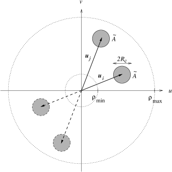
Figure 3: An illustration of the sparse nature of the signal covariance matrix $\mn@boldsymbol{S}$ for interferometer observations.

The reason for the sparse nature of the signal covariance matrix is illustrated in Fig. 3, and is peculiar to observations of the CMB made with interferometers. For simplicity let us consider a single-field observation with no non-coplanar baselines, and focus particularly on two measured visibilities at positions $\mn@boldsymbol{u}_{i}$ and $\mn@boldsymbol{u}_{j}$ respectively in the $uv$-plane. From (4), these visibilities are obtained simply by convolving the underlying independent Fourier modes by the aperture function of the interferometer, which is illustrated by the solid shaded circles in the figure.

Since the extent of the antenna function is determined simply by the physical size of the interferometer horns, it is identically zero outside some critical radius $R_{c}$. Hence one would expect that, if the separation $|\mn@boldsymbol{u}_{i}-\mn@boldsymbol{u}_{j}|$ of the two visibility samples were greater than $2R_{c}$, then the corresponding element $S_{ij}$ of the signal covariance matrix should be identically zero. An additional subtlety remains, however, because the sky is real, and so $a(-\mn@boldsymbol{u},\nu)=a^{*}(\mn@boldsymbol{u},\nu)$. Consequently, correlations exist between areas of the Fourier domain that lie on diametrically opposite sides of the origin of the $uv$-plane; this is illustrated in Fig. 3. Thus, the element $S_{ij}$ of the signal covariance matrix will be identically zero provided $\mn@boldsymbol{u}_{i}$ and $\mn@boldsymbol{u}_{j}$ satisfy both the conditions

$$|\mn@boldsymbol{u}_{i}-\mn@boldsymbol{u}_{j}| > 2R_{c},$$

$$|\mn@boldsymbol{u}_{i}+\mn@boldsymbol{u}_{j}| > 2R_{c}.$$

With reference to Fig. 3, this occurs when no two shaded discs overlap.

We may obtain a simple estimate for the sparsity fraction of the matrix $\mn@boldsymbol{S}$ as follows. Suppose the interferometer samples the $uv$-plane with roughly uniform two-dimensional coverage in the range $\rho_{\rm min}$ to $\rho_{\rm max}$. Thus, given the position of the sample $\mn@boldsymbol{u}_{i}$, a second sample $\mn@boldsymbol{u}_{j}$ may lie anywhere in region between the two concentric circles $\rho=\rho_{\rm min}$ and $\rho=\rho_{\rm max}$ shown in Fig. 3, which is of area $\pi(\rho_{\rm max}^{2}-\rho_{\rm min}^{2})$. In order for $S_{ij}$ to be non-zero, however, $\mn@boldsymbol{u}_{j}$ must lie within a distance $2R_{c}$ of the point $\mn@boldsymbol{u}_{i}$ or $-\mn@boldsymbol{u}_{i}$, which corresponds to an available area $2\pi(2R_{c})^{2}$ of the $uv$-plane. Thus, an estimate of the sparsity fraction $f_{s}$ is given by the ratio of the areas, which reads

$$f_{s}=\frac{8R_{c}^{2}}{\rho_{\rm max}^{2}-\rho_{\rm min}^{2}}.$$

For example, the VSA in compact configuration has $R_{c}\approx 8$, $\rho_{1}\approx 20$ and $\rho_{2}\approx 150$ wavelengths and so the sparsity fraction in this case is $f_{s}\approx 0.02$, i.e. only about 2 per cent of the elements are non-zero.

In fact, the fraction of elements $S_{ij}$ that need be calculated in practice is somewhat smaller than $f_{s}$. As stated above, the element $S_{ij}$ is identically zero if $\mn@boldsymbol{u}_{i}$ and $\mn@boldsymbol{u}_{j}$ satisfy the constraints, with $R_{c}$ equalling the full extent of the aperture function. For most interferometers, however, the aperture function falls close to zero some way before $R_{c}$. Thus, to a very good approximation, $S_{ij}\approx 0$ if

$$|\mn@boldsymbol{u}_{i}-\mn@boldsymbol{u}_{j}| > 2\alpha R_{c},$$ (13)

$$|\mn@boldsymbol{u}_{i}+\mn@boldsymbol{u}_{j}| > 2\alpha R_{c},$$ (14)

where $\alpha$ may be taken to be somewhat less than unity. The resulting sparsity fraction $f_{s}$ is then lowered by a factor $\alpha^{2}$.

In particular, as we describe below, many interferometers have an aperture function that are well described by a (truncated) two-dimensional Gaussian. In this case, we find empirically that an excellent approximation to $\mn@boldsymbol{S}$ is obtained by assuming to be zero all those elements $S_{ij}$ for which (13) and (14) are satisfied, where $\alpha$ is chosen so that $\alpha R_{c}$ corresponds to the radius at which the Gaussian aperture function drops to $1/e$ of its peak central value. This leaves only a very small percentage of matrix elements that must be calculated by evaluating the integrals (11) and (12). On using this approximation for $\mn@boldsymbol{S}$ in the subsequent maximum-likelihood estimation of the CMB power spectrum, discussed later in section 6, we find that the flat band-power estimates obtained in each $\ell$-bin alter by less than 1 per cent, as compared to the case in which we set $\alpha=1$.

4.2 The flat band-power parameterisation

It has become standard practice to parameterise the CMB power spectrum in terms of flat band-powers as follows. The range of $\rho=|\mn@boldsymbol{u}|$ over which we wish to estimate the power spectra of each component is divided into $N_{b}$ separate bins. These bins correspond to separate annuli in the $uv$-plane, centred on the origin. One then assumes that the quantity

$$D^{(p)}(\rho,\nu_{0})\equiv\rho^{2}C^{(p)}(\rho,\nu_{0}),$$

for each physical component $(p=1,2,\ldots,N_{p})$ is constant within any given spectral bin. We denote the constant value of $D^{(p)}(\rho,\nu_{0})$ in the $b$th bin by $\overline{D}_{b}^{(p)}$, and these quantities are the parameters whose values are to be determined from the likelihood analysis described in section 5. Clearly, the total number of parameters is $N_{b}N_{p}$.

This parameterisation of the component power spectra has the advantage that, once the elements of signal covariance matrix have been calculated for one set of band-power values $\overline{D}_{b}^{(p)}$, it may be evaluated for any other set at almost no extra computational cost. This is easily demonstrated by first introducing the top-hat function $T(a,b)$, which equals unity in the range $a\leq\rho<b$ and is zero elsewhere. We may then write $D^{(p)}(\rho,\nu_{0})$ in terms of our model parameters $\overline{D}^{(p)}_{b}$ as

$$D^{(p)}(\rho,\nu_{0})=\sum_{b=1}^{N_{b}}\overline{D}_{b}^{(p)}T(\rho_{b},\rho_{b+1}),$$

where $\rho_{b}$ the lower limit of the $b$th bin. Therefore, the generalised power spectrum $\xi(\rho,\nu_{i},\nu_{j})$ in (10) is now given by

$$\xi(\rho,\nu_{i},\nu_{j})=\frac{1}{\rho^{2}}\sum_{p=1}^{N_{p}}f_{p}(\nu_{i})f_{p}(\nu_{j})\sum_{b=1}^{N_{b}}\overline{D}_{b}^{(p)}T(\rho_{b},\rho_{b+1}).$$

Hence the expressions (11) and (12) can be written as

$$\langle{\cal S}_{j}{\cal S}_{j}^{\ast}\rangle = \sum_{p=1}^{N_{p}}f_{p}(\nu_{i})f_{p}(\nu_{j})\sum_{b=1}^{N_{b}}\overline{D}_{b}^{(p)}K^{(1)}_{ij}(\rho_{b},\rho_{b+1}),$$ (15)

$$\langle{\cal S}_{i}{\cal S}_{j}\rangle = \sum_{p=1}^{N_{p}}f_{p}(\nu_{i})f_{p}(\nu_{j})\sum_{b=1}^{N_{b}}\overline{D}_{b}^{(p)}K^{(2)}_{ij}(\rho_{b},\rho_{b+1}),$$ (16)

where the sets of integrals $K^{(r)}_{ij}(\rho_{b},\rho_{b+1})$ (for $r=1,2$) are given by

$$K^{(r)}_{ij}(\rho_{b},\rho_{b+1})=\int_{\rho_{b}}^{\rho_{b+1}}\frac{{\rm d}\rho}{\rho}W^{(r)}_{ij}(\rho).$$ (18)

As stated earlier, for a given array geometry, the window functions $W^{(r)}_{ij}(\rho)$ $(r=1,2)$ are fixed. Thus the integrals $K^{(r)}_{ij}(\rho_{b},\rho_{b+1})$ need only be evaluated once, at the start of the calculation. Then for any values of the parameters $\overline{D}_{b}^{(p)}$, we may use (15) and (16) to evaluate the elements of the signal covariance matrix $\mn@boldsymbol{S}$.

We may choose the width of the bins arbitrarily, but an obvious choice is the characteristic width of the aperture function of the interferometer (for example, the $1/e$ width). Since this width is the typical correlation length in the convolved Fourier domain, the errors on the derived values of the flat band-powers in different bins will be quasi-uncorrelated. The compact VSA, for example, samples the range $\rho\approx$ 20–150 wavelengths and the aperture function for a single field observation has a $1/e$ width of about $15$ wavelengths. Thus, the total number of spectral bins is $N_{b}\approx 10$.

4.3 Gaussian primary beam

So far we have not assumed a specific form for the primary beam $A(\mn@boldsymbol{x},\nu)$ of the interferometer horns. Nevertheless, for many interferometers, the primary beam may be modelled to a good approximation as a two-dimensional Gaussian. Thus, the primary beam at the $i$th observing frequency $\nu_{i}$ by

$$A(\mn@boldsymbol{x},\nu_{i})=\exp(-|\mn@boldsymbol{x}|^{2}/2\sigma_{i}^{2}),$$

where $\sigma_{i}$ is the dispersion of the primary beam at this frequency. The aperture function is simply the Fourier transform of the primary beam, and is given by

$$\tilde{A}(\mn@boldsymbol{u},\nu_{i})=2\pi\sigma_{i}^{2}\exp(-2\pi^{2}\sigma_{i}^{2}|\mn@boldsymbol{u}|^{2}).$$

As we show in Appendix D, this assumption allows us to obtain analytical expressions for the window functions $W^{(r)}_{ij}(\rho)$ $(r=1,2)$, even for mosaiced observations and including non-coplanar baselines. Thus the integrals $K^{(r)}_{ij}(\rho)$ in (18) can be evaluated quickly and straightforwardly using standard numerical quadrature techniques. For a compact VSA observation of a single field, the calculation of the integrals corresponding to non-zero elements of the signal covariance matrix $\mn@boldsymbol{S}$ require about 2 mins of CPU time.

5 Likelihood analysis

As discussed in the start of section 3.2, the basic data consist of the (real) binned visibility data vector $\mn@boldsymbol{v}$ of length $N_{d}$, and the associated (real) residuals covariance matrix $\mn@boldsymbol{N}=\langle\mn@boldsymbol{n}\mn@boldsymbol{n}^{\rm t}\rangle$. Assuming that the underlying Fourier modes of the sky and the instrumental noise are both Gaussian-distributed with zero mean, the likelihood of obtaining the data, given some particular set of model parameter values $\mn@boldsymbol{a}$, is

$${\cal L}(\mn@boldsymbol{v}|\mn@boldsymbol{a})=\frac{1}{(2\pi)^{N_{d}/2}|\mn@boldsymbol{C}(\mn@boldsymbol{a})|^{1/2}}\exp[-{\textstyle\frac{1}{2}}\mn@boldsymbol{v}^{\rm t}\mn@boldsymbol{C}^{-1}(\mn@boldsymbol{a})\mn@boldsymbol{v}]$$

where $\mn@boldsymbol{C}(\mn@boldsymbol{a})=\mn@boldsymbol{S}(\mn@boldsymbol{a})+\mn@boldsymbol{N}$ is the sum of the signal and noise covariance matrices. In our case, the vector of model parameters $\mn@boldsymbol{a}$ contains the $N_{b}\times N_{p}$ flat band-powers $\overline{D}_{b}^{(p)}$ in each spectral bin for each physical component of sky emission and the structure of the corresponding signal covariance matrix $\mn@boldsymbol{S}(\mn@boldsymbol{a})$ is discussed in the previous section. In fact, in order to avoid numerical instabilities, we adopt the standard technique of working instead with the log-likelihood function

$$\ln{\cal L}(\mn@boldsymbol{v}|\mn@boldsymbol{a})=\mbox{constant}-{\textstyle\frac{1}{2}}\left[\ln|\mn@boldsymbol{C}(\mn@boldsymbol{a})|+\mn@boldsymbol{v}^{\rm t}\mn@boldsymbol{C}^{-1}(\mn@boldsymbol{a})\mn@boldsymbol{v}\right].$$ (19)

The aim of any likelihood analysis is to find the parameter values $\hat{\mn@boldsymbol{a}}$ that maximise the log-likelihood function, and also obtain an estimate of the accuracy with which these parameters have been determined. There exist several different strategies for achieving these goals, which we now discuss, with particular emphasis on the computational cost of each approach when applied to interferometer data.

5.1 Evaluation of the multi-dimensional likelihood

Ideally, one would like to evaluate the full (log-)likelihood function over some hypercube in the space of parameters $\mn@boldsymbol{a}$. In this way, the location of the (global) maximum is obtained immediately, and the presence of multiple subsidiary maxima is readily observed. Also, if one is interested only in (say) the CMB power spectrum, one can integrate out (or marginalise) the parameters describing the power spectrum of Galactic emission in a straightforward manner. Moreover, marginalised distributions for individual parameters can be calculated trivially, in order to obtain confidence limits.

Unfortunately, evaluation of the full likelihood function on a hypercube in parameter space is numerically unfeasible when the number of parameters is large. In our case, the parameter space has $N_{b}N_{p}$ dimensions. Thus, if the likelihood function were evaluated at $M$ points along each parameter axis, the total number of evaluations of the log-likelihood function (19) is $M^{N_{b}N_{p}}$. Even if one assumes that the CMB is the only physical component of emission (i.e. $N_{p}=1$), the dimensionality of the parameter space is equal to the number of spectral bins in which one wishes to estimate the CMB power spectrum. For the latest generation of CMB interferometers $N_{b}\approx 10$, and so the parameter space has a high dimensionality. If, in this case, the likelihood function were calculated at only $M=10$ points on each ‘axis’, this requires $10^{10}$ evaluations of the function (19).

Nevertheless, we note in passing that, with the advent of faster computers and efficient algorithms, it has recently become possible to sample directly from a multidimensional likelihood function using Markov-Chain Monte-Carlo (MCMC) techniques (see e.g. Christensen et al. 2001). Even in a space of large dimensionality, these algorithms allow one to construct accurate one-dimensional marginalised distributions for each parameter, using relatively few evaluations of the likelihood function (typically $\sim\mbox{ few}\times 1000$). The application of MCMC techniques to the estimation of the CMB power spectrum from interferometer data will be presented in a forthcoming paper.

5.1.1 Evaluation of the log-likelihood function

Despite the difficulties associated with the direct calculation of the full likelihood over a hypercube in parameter space, it is necessary for our later discussion to consider the computational task associated with evaluating the log-likelihood function (19) for a given set of parameter values $\mn@boldsymbol{a}$.

First, one must calculate the corresponding covariance matrix $\mn@boldsymbol{C}(\mn@boldsymbol{a})=\mn@boldsymbol{S}(\mn@boldsymbol{a})+\mn@boldsymbol{N}$. Since $\mn@boldsymbol{N}$ is constant, one needs only to calculate the signal covariance matrix $\mn@boldsymbol{S}(\mn@boldsymbol{a})$. As discussed in section 4.2, after evaluating the integrals (18) once, at the start of the calculation, the signal covariance matrix $\mn@boldsymbol{S}(\mn@boldsymbol{a})$, for a given set of parameter values $\mn@boldsymbol{a}$, may be calculated very quickly using (15) and (16). Since, for most interferometers, $\mn@boldsymbol{N}$ is diagonal to a very accurate approximation, $\mn@boldsymbol{C}(\mn@boldsymbol{a})$ inherits the sparse structure of $\mn@boldsymbol{S}(\mn@boldsymbol{a})$ described in section 4.1.

Once $\mn@boldsymbol{C}$ has been calculated, one proceeds to evaluate the log-likelihood function (19), which requires the evaluation of the quadratic form $\mn@boldsymbol{v}^{\rm t}\mn@boldsymbol{C}^{-1}\mn@boldsymbol{v}$ and the determinant $|\mn@boldsymbol{C}|$. The standard procedure is first to perform the Cholesky decomposition

$$\mn@boldsymbol{C}=\mn@boldsymbol{LL}^{\rm t},$$ (20)

where $\mn@boldsymbol{L}$ is a lower triangular matrix. The determinant $|\mn@boldsymbol{C}|$ is then given by

$$|\mn@boldsymbol{C}|=|\mn@boldsymbol{L}\mn@boldsymbol{L}^{\rm t}|=|\mn@boldsymbol{L}|^{2},$$

where, since $\mn@boldsymbol{L}$ is lower triangular, $|\mn@boldsymbol{L}|$ is simply the product of its diagonal elements. To evaluate the quadratic form, one then solves for $\mn@boldsymbol{x}$ the lower triangular system

$$\mn@boldsymbol{Lx}=\mn@boldsymbol{v},$$ (21)

which is computationally straightforward. Finally, one forms the scalar product of $\mn@boldsymbol{x}$ with itself to obtain

$$\mn@boldsymbol{x}^{\rm t}\mn@boldsymbol{x}=\mn@boldsymbol{v}^{\rm t}(\mn@boldsymbol{L}^{-1})^{\rm t}\mn@boldsymbol{L}^{-1}\mn@boldsymbol{v}=\mn@boldsymbol{v}^{\rm t}(\mn@boldsymbol{L}\mn@boldsymbol{L}^{\rm t})^{-1}\mn@boldsymbol{v}=\mn@boldsymbol{v}^{\rm t}\mn@boldsymbol{C}^{-1}\mn@boldsymbol{v}.$$

By far the most computationally intensive step in the calculation is the Cholesky decomposition (20). For a compact VSA observation of a single field, for example, the (real) binned visibility data vector $\mn@boldsymbol{v}$ contains about $N_{d}=5000$ elements, so that $\mn@boldsymbol{C}$ has dimensions $5000\times 5000$. Using a standard lapack subroutine (Anderson et al. 1999) to perform the decomposition requires about 5 mins of CPU time. The subsequent solution of the lower-triangular system (21) is much faster, requiring only 0.25 secs of CPU time. Hence, the total time required to evaluate the log-likelihood function (19) for a given set of parameters $\mn@boldsymbol{a}$ is around 5 mins. We therefore see that the evaluation of the full likelihood function over some hypercube in parameter space is computationally unfeasible.

We note, in passing, that the lapack library uses the highly-optimised Basic Linear Algebra Subroutines (blas) for simple operations. In practice, this combination provides the fastest readily-available dense matrix computational subroutines. As a comparison, performing the same calculation of the log-likelihood using simple unoptimised routines, such as those presented in Press et al. (1994), required approximately 20 times the CPU time on an equivalent processor.

5.1.2 Sparse matrix conjugate-gradient algorithm

As stated earlier, the covariance matrix $\mn@boldsymbol{C}$ is very sparse for interferometer data. Therefore, using standard dense matrix subroutines, such as those in the lapack library, is wasteful both computationally and in terms of memory usage. One should instead employ sparse matrix algorithms, which take advantage of the sparse structure of $\mn@boldsymbol{C}$ and require only the storage of its non-zero elements (plus an integer array to store their positions in the matrix). It was found that the most computationally efficient approach was to solve the linear system

$$\mn@boldsymbol{Cx}=\mn@boldsymbol{v},$$ (22)

with a preconditioned conjugate-gradient algorithm that performed its internal matrix and vector operations using sparse matrix routines. In particular, the preconditioner was chosen to be the sparse incomplete Cholesky decomposition of $\mn@boldsymbol{C}$. This matrix has the form

$$\tilde{\mn@boldsymbol{C}}=\mn@boldsymbol{L}\mn@boldsymbol{D}\mn@boldsymbol{L}^{\rm t},$$ (23)

where $\mn@boldsymbol{D}$ is a diagonal matrix, and $\mn@boldsymbol{L}$ is lower triangular with unit diagonal elements and which has the same sparse structure as the lower triangle of $\mn@boldsymbol{C}$ (which is symmetric). Since one imposes this sparse structure on $\mn@boldsymbol{L}$, the matrix $\tilde{\mn@boldsymbol{C}}$ is only an approximation to $\mn@boldsymbol{C}$ (see Greenbaum 1997). Nevertheless, the approximation is sufficiently accurate to provide an extremely effective preconditioner, which allows the conjugate-gradient algorithm to converge to the solution $\mn@boldsymbol{x}$ in a just a few iterations. Moreover, it was found that the preconditioner $\tilde{\mn@boldsymbol{C}}$ was a sufficiently accurate approximation to $\mn@boldsymbol{C}$ that the determinant

$$|\tilde{\mn@boldsymbol{C}}|=|\mn@boldsymbol{L}\mn@boldsymbol{D}\mn@boldsymbol{L}^{\rm t}|=|\mn@boldsymbol{L}||\mn@boldsymbol{D}||\mn@boldsymbol{L}^{\rm t}|=|\mn@boldsymbol{D}|,$$

differed by less than 0.01 per cent from the true determinant $|\mn@boldsymbol{C}|$. Since $\mn@boldsymbol{D}$ is diagonal, its determinant is trivially evaluated. Thus, the sparse matrix preconditioned conjugate-gradient algorithm provides an efficient method of calculating the complete log-likelihood function (19).

As in the dense matrix approach, the most computationally demanding step of the calculation is the construction of the incomplete Cholesky preconditioner (23). As an example, for the $5000\times 5000$ covariance corresponding to a compact VSA observation of a single field, the calculation requires about 30 sec of CPU time. The subsequent preconditioned conjugate-gradient solution of the linear system (22) then requires only about 0.5 sec of CPU time. Thus, we see that, in this case, the evaluation of the log-likelihood function by this method is approximately 10 times faster than the standard dense matrix approach using lapack subroutines. For larger problems, the lapack routines scale as $O(N_{d}^{3})$, where $N_{d}$ is the size of the data vector, whereas the sparse matrix algorithm scales as $O(f_{s}^{3/2}N_{d}^{3})$, where $f_{s}$ is the sparsity fraction of the covariance matrix $\mn@boldsymbol{C}$. Unfortunately, the speed-up provided by the sparse matrix approach is still insufficient to enable the calculation of the full likelihood distribution over some hypercube in parameter space.

5.2 Numerical maximisation of the likelihood

When it is unfeasible to calculate the full likelihood function directly over the parameter space, one usually resorts to numerical maximisation. The main disadvantage of this approach is that most standard methods will converge to the nearest local maximum, which need not be the global maximum. One would hope, however, that the likelihood function is sufficiently structureless that this is not a problem for a reasonable starting guess for the CMB power spectrum.

Standard numerical maximisation (minimisation) algorithms use differing amounts of gradient and/or curvature information in order to arrive at the maximum point. For example, methods such as the downhill simplex or Powell’s direction-set algorithm use no gradient information, requiring only function evaluations (see Press et al. 1994). Other methods, such as the variable metric technique, use only gradient information, whereas the standard Newton–Raphson algorithm requires both gradient and curvature information. In particular, Newton–Raphson technique and Powell’s direction-set algorithm were investigated as methods of numerically maximising the likelihood function.

5.2.1 The Newton–Raphson method

The Newton–Raphson method (or variations thereon) is the standard numerical minimisation technique used in maximum-likelihood estimation of the CMB power spectrum (e.g. Borrill 1999). Starting from some initial guess $\mn@boldsymbol{a}_{0}$ for the flat band-powers, one performs the iteration

$$\mn@boldsymbol{a}_{n+1}=\mn@boldsymbol{a}_{n}+\delta\mn@boldsymbol{a}_{n},$$ (24)

where the correction $\delta\mn@boldsymbol{a}_{n}$ is given by

$$\delta\mn@boldsymbol{a}_{n}=-[\mn@boldsymbol{H}^{-1}\mn@boldsymbol{g}]_{\mn@boldsymbol{a}=\mn@boldsymbol{a}_{n}},$$

in which $\mn@boldsymbol{g}=\nabla(\ln{\cal L})$ is the gradient vector and $\mn@boldsymbol{H}=\nabla\nabla(\ln{\cal L})$ is the curvature (or Hessian) matrix. The iteration (24) is continued until the algorithm has converged to the required accuracy. The elements of the gradient vector and curvature matrix of the log-likelihood function (19) are easily shown to be given respectively by

$${\partial\ln{\cal L}\over\partial a_{k}} = {\textstyle\frac{1}{2}}\left[\mn@boldsymbol{v}^{\rm t}\mn@boldsymbol{C}^{-1}{\partial\mn@boldsymbol{S}\over\partial a_{k}}\mn@boldsymbol{C}^{-1}\mn@boldsymbol{v}-\mbox{Tr}\left(\mn@boldsymbol{C}^{-1}{\partial\mn@boldsymbol{S}\over\partial a_{k}}\right)\right],$$ (25)

$${\partial^{2}\ln{\cal L}\over\partial a_{k}\partial a_{k}^{\prime}} = -\mn@boldsymbol{v}^{\rm t}\mn@boldsymbol{C}^{-1}{\partial\mn@boldsymbol{S}\over\partial a_{k}}\mn@boldsymbol{C}^{-1}{\partial\mn@boldsymbol{S}\over\partial a_{k^{\prime}}}\mn@boldsymbol{C}^{-1}\mn@boldsymbol{v}$$ (26)

$$\qquad\qquad+{\textstyle\frac{1}{2}}\mbox{Tr}\left(\mn@boldsymbol{C}^{-1}{\partial\mn@boldsymbol{S}\over\partial a_{k}}\mn@boldsymbol{C}^{-1}{\partial\mn@boldsymbol{S}\over\partial a_{k^{\prime}}}\right),$$

where $\mbox{Tr}(\,)$ denotes the trace of a matrix.

The implementation of the Newton–Raphson algorithm can be divided neatly into a series of computational steps (see Borrill 1999). For the analysis of interferometer data, each iteration of the algorithm consists of the following steps.

1. Calculation of the signal covariance derivative matrices $\partial\mn@boldsymbol{S}/\partial a_{k}$ $(k=1,\ldots,N)$, where $N$ is the total number of parameters. In the flat band-power parameterisation of the power spectra, we see from (15) and (16) that $\mn@boldsymbol{S}$ is linear in the parameters $\mn@boldsymbol{a}$. Thus, the derivative matrices are simply appropriate linear combinations of the integrals $K_{ij}^{(a)}$ in (18), which are evaluated once at the start of the calculation.

2. Construction of the (sparse) covariance matrix

   $$\mn@boldsymbol{C}=\mn@boldsymbol{N}+\sum_{k=1}^{N}a_{k}{\partial\mn@boldsymbol{S}\over\partial a_{k}},$$

   calculation of its (incomplete) Cholesky decomposition and solution of the linear system $\mn@boldsymbol{Cx}=\mn@boldsymbol{v}$.

3. Solution of the linear systems

   $$\mn@boldsymbol{CY}_{k}={\partial\mn@boldsymbol{S}\over\partial a_{k}}\qquad(k=1,\ldots,N),$$

   where $\mn@boldsymbol{Y}_{k}$ is a matrix of the same dimensions as $\mn@boldsymbol{C}$. Each column of $\mn@boldsymbol{Y}_{k}$ is solved for using the (incomplete) Cholesky decomposition obtained in step (ii).

4. Assemble the elements of the gradient vector

   $$g_{k}\equiv{\partial\ln{\cal L}\over\partial a_{k}}={\textstyle\frac{1}{2}}\left[\mn@boldsymbol{v}^{\rm t}\mn@boldsymbol{Y}_{k}\mn@boldsymbol{x}-\mbox{Tr}(\mn@boldsymbol{Y}_{k})\right].$$

5. Assemble the elements of the curvature matrix

   $$H_{kk^{\prime}}\equiv{\partial^{2}\ln{\cal L}\over\partial a_{k}\partial a_{k^{\prime}}}=-\mn@boldsymbol{v}^{\rm t}\mn@boldsymbol{Y}_{k}\mn@boldsymbol{Y}_{k^{\prime}}\mn@boldsymbol{x}+{\textstyle\frac{1}{2}}\mbox{Tr}(\mn@boldsymbol{Y}_{k}\mn@boldsymbol{Y}_{k^{\prime}}).$$

6. Calculate the correction vector $\delta\mn@boldsymbol{a}=-\mn@boldsymbol{H}^{-1}\mn@boldsymbol{g}$.

Although it is not necessary for the Newton–Raphson algorithm, we note that in step (ii) one performs all the necessary calculations to evaluate the log-likelihood function $\ln{\cal L}$ itself. This can be useful for checking that its value is, in fact, decreasing with each iteration. Typically, the Newton–Raphson algorithm converges to the maximum-likelihood solution in approximately 5 iterations.

The computationally most demanding calculations in each iteration are steps (ii) and (iii) above, which may be performed using either the dense or sparse matrix techniques discussed in the previous section. As mentioned in section 5.1, for a visibility data vector $\mn@boldsymbol{v}$ of length 5000, the calculation in step (ii) of the (incomplete) Cholesky decomposition requires approximately 5 min of CPU time for the dense matrix lapack routines and about 30 sec for the sparse matrix algorithm. The subsequent solution of the linear system $\mn@boldsymbol{Cx}=\mn@boldsymbol{v}$ then requires about 0.25 sec or 0.5 sec respectively. Thus, it would clearly be faster to use the sparse matrix technique in step (ii).

In step (iii), however, one must solve a large number of linear systems, namely one for each column of $\mn@boldsymbol{Y}_{k}$ for $k=1,\ldots,N$, using the (incomplete) Cholesky decomposition calculated in step (ii). Even assuming the sky emission is due only to the CMB, the total number of linear systems is $N_{d}N_{b}$, where $N_{d}$ is the length of the data vector $\mn@boldsymbol{v}$ and $N_{b}$ is the number of spectral bins in which one wishes to calculate the CMB power spectrum. For a compact VSA observation of a single field, $N_{d}\approx 5000$ and $N_{b}\approx 10$, and so one must solve $\sim 50000$ linear systems. Solving each system requires around 0.5 sec of CPU time using the sparse conjugate-gradient algorithm, but only 0.25 secs using the lapack dense matrix routines. Taking step (ii) and step (iii) together, it is therefore faster to use the lapack routines, which require a total of about 3.5 hrs CPU time to complete these steps. The remaining steps (iv) – (vi) require only around 0.5 hr of CPU time, so that a full Newton–Raphson iteration takes around 4 hrs. Since 5 iterations of the Newton–Raphson algorithm are typically required for convergence, the total CPU to calculate the maximum-likelihood solution is around 20 hrs.

We note that Bond, Jaffe & Knox (1998, 2000) propose a variant of the Newton–Raphson algorithm, in which steps (v) and (vi) are different. In particular, the correction vector in step (vi) is replaced by

$$\delta\mn@boldsymbol{a}=-\mn@boldsymbol{F}^{-1}\mn@boldsymbol{g},$$

where the Fisher matrix $\mn@boldsymbol{F}$ is the expectation value of the curvature matrix. From (26), the Fisher matrix has the elements

$$F_{kk^{\prime}}\equiv\langle H_{kk^{\prime}}\rangle={\textstyle\frac{1}{2}}\mbox{Tr}\left(\mn@boldsymbol{C}^{-1}{\partial\mn@boldsymbol{S}\over\partial a_{k}}\mn@boldsymbol{C}^{-1}{\partial\mn@boldsymbol{S}\over\partial a_{k^{\prime}}}\right).$$

Thus, step (v) above is replaced by

$$F_{kk^{\prime}}={\textstyle\frac{1}{2}}\mbox{Tr}(\mn@boldsymbol{Y}_{k}\mn@boldsymbol{Y}_{k^{\prime}}).$$ (27)

Comparing the expressions for $H_{kk^{\prime}}$ and $F_{kk^{\prime}}$ we see that some saving is made by using the latter. From (27), however, we note that the calculation of the Fisher matrix still requires knowledge of the matrices $\mn@boldsymbol{Y}_{k}$ $(k=1,\ldots,N)$ calculated in step (iii), which is the computationally most demanding part of the calculation. Hence, the use of the Fisher matrix, rather than the full curvature matrix, leads to a reduction of only around 20 mins in the CPU time required for each Newton–Raphson iteration.

5.2.2 Powell’s direction-set method

Clearly, the Newton–Raphson algorithm described above is computationally intensive. Moreover, most time is spent is computing quantities necessary for calculating the gradient and/or curvature of the log-likelihood function. As discussed in section 5.1.2, however, the log-likelihood function itself can be calculated using the sparse preconditioned conjugate-gradient method in about one-tenth of the CPU time required by the standard lapack dense matrix routines. These observations suggest that it might be more computationally efficient to maximise the log-likelihood function using an algorithm that requires only function calls, rather than gradient and curvature information.

A particularly efficient and robust estimator of this type is Powell’s direction-set method, which is described in detail by Press et al. (1994). At each iteration, the algorithm determines a set of ‘conjugate’ directions at the corresponding point $\mn@boldsymbol{a}$ in the parameter space, and minimises the function along each direction in turn. The method can be shown to be quadratically convergent, so that an exact quadratic form would be minimised in $N(N+1)$ line-minimisation, where $N$ is the dimensionality of the parameter space. Typically, each line-minimisation requires 2 or 3 function calls. Thus, one would expect between $2N(N+1)$ and $3N(N+1)$ functions calls would be required to minimise an exact quadratic form.

Since the algorithm requires only function evaluations, one may straightforwardly employ the sparse matrix technique discussed in section 5.1.2 for evaluating the log-likelihood function. Assuming the sky emission to be due solely to the CMB, the dimensionality of the parameter space is simply the number of spectral bins in which one wishes to estimate the CMB power spectrum, i.e. $N=N_{b}$. For a compact VSA observation of a single field, $N_{b}\approx 10$ and it was found that the algorithm converged to the maximum-likelihood solution after $\approx 300$ evaluations of the likelihood function. This is in broad agreement with the anticipated number of function evaluations quoted above, although the presence of the term $\ln|\mn@boldsymbol{C}|$ in the log-likelihood function (19) means that it is not a simple quadratic form. Thus, since each function evaluation requires 30 sec of CPU time, the maximum-likelihood CMB power spectrum may be obtained in about 2.5 hrs of CPU time, which is considerably faster than the Newton–Raphson algorithm.

We note, in passing, that the downhill-simplex minimisation algorithm (see Press et al. 1994) was also investigated. This again uses only function calls, but it was found to converge too slowly. Nevertheless, a robust technique for obtaining a accurate minimum in a reasonable amount of CPU time is first to employ Powell’s direction-set algorithm until it converges to some point $\hat{\mn@boldsymbol{a}}$ in parameter space, and then to restart the minimisation process from this point using a downhill simplex. The final simplex step is then very fast and provides a robust estimate of the minimum point. This algorithm is implemented as the program maxlike in the Microwave Anisotropy Dataset Computational sOftWare (madcow) package (see section 5.4).

5.2.3 Estimation of errors on parameter values

A major disadvantage of numerically maximising the likelihood is that one remains ignorant of the global shape of the distribution. Therefore, one cannot calculate marginalised distributions for each parameter, in order to obtain proper confidence limits. Nevertheless, one would hope that the shape of the likelihood function ${\cal L}$ near its peak $\hat{\mn@boldsymbol{a}}$ should be well-approximated by a Gaussian, so that

$$\ln{\cal L}(\hat{\mn@boldsymbol{a}}+\delta\mn@boldsymbol{a})=\ln{\cal L}(\hat{\mn@boldsymbol{a}})+{\textstyle\frac{1}{2}}\delta\mn@boldsymbol{a}^{\rm t}\mn@boldsymbol{H}(\hat{\mn@boldsymbol{a}})\delta\mn@boldsymbol{a},$$ (28)

where $\mn@boldsymbol{H}$ is the curvature (or Hessian) matrix given in (26), and the gradient term in the Taylor expansion vanishes since $\hat{\mn@boldsymbol{a}}$ is a maximum. Exponentiating (28), we immediately recognise that covariance matrix of our errors is given simply by the inverse of the curvature matrix at the peak,

$$\langle\delta\mn@boldsymbol{a}\,\delta\mn@boldsymbol{a}^{\rm t}\rangle=\mn@boldsymbol{H}^{-1}(\hat{\mn@boldsymbol{a}}).$$

The curvature matrix $H(\hat{\mn@boldsymbol{a}})$ may be calculated directly by performing steps (ii), (iii) and (v) in the Newton–Raphson algorithm at the maximum point $\hat{\mn@boldsymbol{a}}$. From section 5.2.1, we note that, for a compact VSA observation of a single field with 10 spectral bins, this requires about 4 hrs of CPU time. However, we find that a computationally more efficient procedure is to calculate the curvature matrix numerically by performing second differences along each parameter direction. An appropriate step size is easily chosen, and the algorithm requires ${\textstyle\frac{1}{2}}N(N+3)+1$ function evaluations. Thus, for 10 spectral bins, one must evaluate the log-likelihood function around 70 times. Using the sparse preconditioned conjugate-gradient algorithm, this requires only about 30 mins of CPU time. Comparing the resulting curvature matrix with that obtained directly from (26), we find that each element is agrees to within 0.1 per cent. The numerical calculation of the curvature matrix and its inversion to produce the errors covariance matrix is implemented in the routine errors in the madcow package.

5.3 Evaluation of the likelihood function along parameter axes

The Powell direction-set minimiser, together with the sparse preconditioned conjugate-gradient algorithm for evaluating the log-likelihood function, provides a method of obtaining the maximum-likelihood power spectrum and the errors covariance matrix in a reasonable amount of CPU time. Nevertheless, by taking full advantage of the sparse nature of the visibilities covariance matrix $\mn@boldsymbol{C}$ and of the flat band-power parameterisation of the power spectrum, it is possible to calculate the maximum-likelihood solution in considerably less computing time.

In the flat band-power parameterisation, one divides the observed $\rho$-range into spectral bins of width $\Delta\rho$. This corresponds to dividing the $uv$-plane into a set of concentric annuli in each of which the power spectrum $D^{(p)}(\rho)=\rho^{2}C^{(p)}(\rho,\nu_{0})$ of each physical component in assumed constant, and its amplitude is the parameter to be determined. A typical annulus is illustrated by the solid circles in Fig. 4, which are overlayed on the visibilities samples shown in Fig. 2. The extent of the aperture function for a compact VSA observation of a single field is plotted as the solid disc in the figure.

Figure 4: An illustration of a typical annulus in the $uv$-plane, with which the power spectrum is assumed constant (solid circles). This is overlayed on the binned visibility samples shown in Fig. 2. The aperture function is plotted as a solid disc. Only visibilities lying in the region between the two dashed circles are sensitive to the level of the power spectrum in the annulus.

As discussed in section 2.2, an interferometer visibility measurement is only sensitive to the underlying sky Fourier modes that lie within the aperture function at that point in the $uv$-plane. Thus, only a fraction of the total number of measured visibilities are sensitive to the amplitude of the power spectrum (of either the CMB or some foreground component) in a particular annulus. This is illustrated in Fig. 4, where only the visibilities lying in the region between the two dashed circles are sensitive to the level of the power spectrum in our typical annulus.

Thus, provided one is calculating the log-likelihood function along the ‘axes’ in parameter space, so that only one parameter value is changing at any one time, the effective size of the dataset is much smaller than the total number of data points. Thus, if the parameters $a_{k^{\prime}\neq k}$ are fixed,

$$\ln{\cal L}(\mn@boldsymbol{v}|a_{k})=\ln{\cal L}(\tilde{\mn@boldsymbol{v}}_{k}|a_{k}),$$

where $\tilde{\mn@boldsymbol{v}}_{k}$ is the reduced data vector consisting of only those visibilities sensitive to the flat band-power $a_{k}$. Given the geometry illustrated in Fig. 4, the length of the reduced data vector will, in general, depend on the radius of the corresponding $uv$-annulus, the extent of the aperture function and the positions of the measured visibilities in the $uv$-plane. For a compact VSA observation of a single field, using $N_{b}=10$ spectral bins (or $uv$-annuli), the reduced data vector typically contains around 3–10 times fewer data points than the full data vector.

The smaller size of the reduced data vector, as compared to the full data vector, leads to a significant increase in the speed with which the log-likelihood function can be calculated along the axes in parameter space. For the standard lapack dense matrix routines, the cost of evaluating the log-likelihood function scales as $O(N_{d}^{3})$, where $N_{d}$ is the length of the data vector. Thus, by using the reduced data vector, the computation time for evaluating the log-likelihood function is reduced by a factor between 30 and 1000, depending on the annulus in question.

Unfortunately, the same speed-up factor is not obtained for the sparse preconditioned conjugate-gradient algorithm. This reason for this is clear from Fig. 4. Since the reduced data vector contains only visibilities lying in the region between the two dashed circles, the corresponding sparsity fraction $f_{s}$, will increase significantly. Since the sparse matrix algorithm scales as $O(f_{s}^{3/2}N_{d}^{3})$, the log-likelihood evaluation is speed up only by a factor between 4–60, depending on the annulus. Nevertheless, for a compact VSA observation of a single field, the sparse matrix approach is still about a factor of 3 times faster in evaluating the log-likelihood function than the lapack dense matrix algorithm, when timings are averaged over the 10 spectral bins.

5.3.1 Calculation of the maximum-likelihood solution

The speed-up outlined above is only possible when one varies only a single parameter $a_{k}$, while keeping the others fixed. Thus, one cannot use a general minimisation algorithm such as the Newton–Raphson or Powell direction-set method, since these perform iterations of the form

$$\mn@boldsymbol{a}_{n+1}=\mn@boldsymbol{a}_{n}+\delta\mn@boldsymbol{a}_{n},$$

where $\delta\mn@boldsymbol{a}_{n}$ may be in some general direction in parameter space. A straightforward solution is provided, however, simply by using a restricted version the Powell direction-set algorithm in which the ‘conjugate’ directions are forced to remain along the parameter axes. Starting with some initial guess $\mn@boldsymbol{a}_{0}$ for the solution, this procedure is equivalent to performing, in turn, independent line-minimisations along each parameter axis, while keeping the other parameters fixed at their initial values. One then updates the whole solution vector and repeats the process until convergence is obtained. It was found that the likelihood function was sufficiently structureless that this restricted ‘Powell’ algorithm still converged in around $3N(N+1)$ functions evaluations, where $N$ is the number of parameters $\mn@boldsymbol{a}$.

For a compact VSA observation of a single field, with 10 spectral bins, the maximum-likelihood power spectrum is obtained in about 10 mins of CPU time using the sparse matrix evaluation of the log-likelihood function, or about 45 mins using standard lapack dense matrix routines. In both cases, this is clearly faster than either of the methods discussed in section 5.2, and is hence our method of choice for determining the maximum-likelihood power spectrum from the current generation of CMB interferometers. The sparse and dense matrix versions of the algorithm are implemented respectively in the programs spfastlike and lafastlike in the madcow package.

5.3.2 Estimation of errors on parameter values

Once the maximum-likelihood solution $\hat{\mn@boldsymbol{a}}$ has been obtained, it still remains to calculate the errors on our estimated flat band-powers. One can, of course, simply calculate the curvature matrix $\mn@boldsymbol{H}(\hat{\mn@boldsymbol{a}})$ numerically, in the manner discussed in section 5.2.3, which requires about 30 mins of CPU time for a compact VSA observation of a single field, with 10 spectral bins. This approach does, however, assume that the likelihood function is well-approximated by a Gaussian near its peak, and leads to symmetric error bars on our estimated parameter values. This may not, in fact, be a valid approximation, especially for poorly constrained parameters.

An alternative approach is to make use of the fact that it is usual to choose the width $\Delta\rho$ of the spectral bins to correspond to the characteristic width of the aperture function in the $uv$-plane. Let us suppose that the sky emission is due only to the CMB. In this case, all the flat band-power estimates $\hat{\mn@boldsymbol{a}}$ will be close to uncorrelated. This is equivalent to the eigenvectors of $\mn@boldsymbol{H}(\hat{\mn@boldsymbol{a}})$ lying close to the directions of the axes in parameter space, and the off-diagonal elements being very small as compared with those on the leading diagonal. In this case, a better representation of the errors on our estimates is obtained by evaluating the log-likelihood function along each parameter direction in turn, through the point $\hat{\mn@boldsymbol{a}}$. Thus is illustrated in Fig. 5. In the ideal case, where the parameters $a_{k}$ $(k=1,\ldots,N)$ are independent, the resulting curves would be the marginal distributions of each parameter.

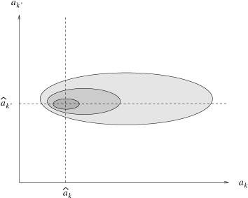
Figure 5: An illustration of calculating the likelihood function along each parameter direction, through the peak $\hat{\mn@boldsymbol{a}}$.

In order to obtain accurate confidence intervals on each parameter, it is best to calculate the log-likelihood function at a large number of points along each parameter direction. Although, using the reduced data vector approach discussed above, it is relatively cheap to evaluate the log-likelihood function along each parameter direction (while keeping the other parameters fixed), if one desires more than around 100 points along each direction, a more efficient procedure is to rotate to the signal-to-noise eigenbasis for each parameter $a_{k}$ in turn, as discussed in Appendix E. Once this rotation has been performed for a given parameter $a_{k}$, the log-likelihood function can be calculated at a large number of points along this parameter direction at virtually no additional computational cost.

Rotating to the signal-to-noise eigenbasis requires the solution of a generalised eigenproblem of dimension equal to the length of the reduced data vector $\tilde{\mn@boldsymbol{v}}_{k}$ for each parameter. In the absence of a stable sparse matrix implementation of this algorithm, a standard lapack subroutine was used to perform the calculation. For a compact VSA observation of a single field, with 10 spectral bins, the entire calculation requires about 30 mins of CPU time. This approach is implemented as the routine eigenlike in the madcow package.

In fact, the routine eigenlike may be used in isolation to obtain both the maximum-likelihood solution $\hat{\mn@boldsymbol{a}}$, and the likelihood functions along each parameter direction passing through the maximum. Starting with some initial guess $\mn@boldsymbol{a}_{0}$ one performs a single ‘iteration’ by calculating the likelihood functions along the parameter directions through $\mn@boldsymbol{a}_{0}$. The peak position of the likelihood in each direction is then used to update the solution vector and the process is repeated until it converges. For observations of a single field convergence is usually achieved after only 3 iterations. Thus, for a compact VSA observation of a single field, with 10 spectral bins, the full calculation requires about 1.5 hrs of CPU time. This is clearly slower than using spfastlike or lafastlike, but provides a useful cross check of one’s results, since it uses entirely different computational subroutines.

5.3.3 Marginalisation over Galactic parameters

For illustration, we assumed above that the sky emission was due solely to CMB fluctuations, without any contaminating Galactic foreground emission. Let us now suppose instead that there is, in fact, substantial foreground emission coming from (say) a single Galactic component. If multifrequency observations are available, one may calculate the maximum-likelihood solution $\hat{\mn@boldsymbol{a}}$ for the CMB and Galactic flat band-powers in each spectral bin, using any of the techniques outlined above.

Suppose the parameters $a_{k}$ and $a_{k^{\prime}}$ correspond respectively to the CMB and Galactic flat band-powers in the $k$th spectral bin. If the bin width corresponds to the extent of the aperture function, these two parameters will be quasi-uncorrelated with the remaining ones, but the parameters $a_{k}$ and $a_{k^{\prime}}$ themselves will be strongly correlated since they refer to the same spectral bin. Nevertheless, the routine eigenlike provides a natural method for marginalising over the flat band-power of the Galactic (or CMB) component in each bin. Keeping the parameters $a_{k^{\prime\prime}}$ ($k^{\prime\prime}\neq k$ and $k^{\prime\prime}\neq k^{\prime}$) fixed, one can calculate the log-likelihood function in the two-dimensional $(a_{k},a_{k^{\prime}})$-space by performing a signal-to-noise eigenmode rotation at each required value of $a_{k^{\prime}}$ (say), and calculating the variation with respect to $a_{k}$ at almost no extra computational cost. One can then perform a numerical integration over $a_{k}$ or $a_{k^{\prime}}$, thereby obtaining a marginalised likelihood function for the other parameter.

5.4 Implementation: the madcow package

The Microwave Anisotropy Dataset Computational sOftWare (madcow) package consists of the 5 programs maxlike, errors, spfastlike, lafastlike and eigenlike, which are discussed above. The first three programs are based on the sparse matrix conjugate-gradient algorithm for calculating the log-likelihood function, discussed in section 5.1.2, whereas the last two programs calculate the log-likelihood function using lapack subroutines.

All the above programs have been parallelised using MPI, in order that they may be run on distributed-memory parallel machines. The parallelisation of the routines lafastlike and eigenlike makes use of the Scalapack parallel version of the lapack library. The speed of both routines is found to scale linearly with the number of processors up to the maximum of 8 CPUs available on the Linux Beowulf cluster at our disposal. The parallelisation of the spare matrix programs maxlike.c, errors.c and spfastlike.c is less straightforward, since existing parallel versions of the relevant routines are not available. Some parallelisation of the algortihms has been performed, but the resulting programs do not scale as effectively as those using lapack routines. A method of achieving linear scaling of the sparse matrix algorithm is currently under investigation. A $\beta$-test version of the madcow package may be downloaded from http://www.mrao.cam.ac.uk/software/madcow/.

6 Application to simulated observations

As an illustration of our maximum-likelihood methods, in this section we apply them to simulated VSA observations. The VSA is a 14-element radio interferometer, which is capable of operating at frequencies between 26 and 36 GHz. The VSA is currently observing at a frequency of 34.1 GHz. Its observing bandwidth is 1.5 GHz, and the system temperature about 25-35 K. The telescope can observe in two different configurations: the compact array uses corrugated horn-reflector antennas of 14.3 cm diameter and baselines up to 1.5 m, and the extended array consists of 32.2-cm horns with baselines up to about 3 m. We base our simulations on the compact array with the actual antenna arrangement as of June 2001, as shown in Fig. 6. The primary (power) beam has a FWHM of 4.6 degrees at 34.1 GHz and can be well approximated by a Gaussian (Fig. 7).

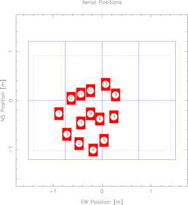
Figure 6: The VSA compact array in June 2001. The rectangular area indicates the shape of the lower part of the VSA table, which is mounted in east–west direction and steerable in elevation. There are 14 horn–reflector antennas mounted at an inclination of 35 degrees. The dashed lines above the horns show the extension of the antenna mount (Rusholme 2001).

Figure 7: The VSA primary (power) beam profile (dashed line) at 34.1 GHz calculated by a ray-tracing program for the corrugated horn-reflector antennas, compared to a Gaussian (solid line) of the same FWHM (4.6 degrees).

We simulate VSA observations of three fields centred on ${\rm RA}(1950)=0^{\rm h}~{}20^{\rm m}~{}00.0^{\rm s}$, ${\rm Dec.}~{}(1950)=30^{\circ}~{}00^{\prime}~{}00^{\prime\prime}$, ${\rm RA}(1950)=0^{\rm h}~{}07^{\rm m}~{}20.6^{\rm s}$, ${\rm Dec.}~{}(1950)=30^{\circ}~{}16^{\prime}~{}30^{\prime\prime}$ and ${\rm RA}(1950)=0^{\rm h}~{}12^{\rm m}~{}50.0^{\rm s}$, ${\rm Dec.}~{}(1950)=27^{\circ}~{}48^{\prime}~{}00^{\prime\prime}$ (the VSA1, VSA1A and VSA1B fields respectively). Real VSA observations of these fields (and others) have been completed and are currently being analysed. The $uv$-coverage for a 5 h-observation of the VSA1 field was shown in Fig. 1(c). The antenna arrangement yields a reasonably uniform sampling in the multipole region $\ell\approx 100-900$.

In order to simulate an observation of CMB fluctuations, we first create a $512\times 512$ array of Fourier modes, the real and imaginary parts of which are drawn from a Gaussian distribution with a variance given by a theoretical power spectrum corresponding to a standard inflationary CDM model with a Hubble parameter $H_{0}=$ 65 km s^-1 Mpc^-1 and a fractional baryon density $\Omega_{\rm b}=0.05$. The model is spatially-flat with $\Omega_{\rm m}=0.3$ and $\Omega_{\Lambda}=0.7$, a primordial scalar spectral index $n=1$ and no tensor modes. The spectrum is normalised such that $Q_{\rm rms}=18\mu$K. The theoretical $C_{l}$ spectrum is plotted in Fig. 8, and the actual realisation of the CMB Fourier modes were plotted in Fig. 1(a).

Figure 8: The theoretical CDM power spectrum with parameter values described in the text.

These Fourier modes are inverse Fourier-transformed to obtain the corresponding CMB anisotropies on the sky. This array is then multiplied by the telescope primary beam and Fourier transformed to give a regular array in the visibility plane (see Fig. 1(b)). A VSA observation is then simulated by sampling the regular array at the required points in the $uv$-plane using a bilinear interpolation. The $uv$-positions at which the visibilities are sampled correspond to a 64-s integration per visibility (see Fig. 1(c)).

Instrumental noise on the data is simulated by adding to each visibility a random complex number for which the real and imaginary parts are drawn from a Gaussian distribution with an rms of 3.5 Jy. Since the measured VSA noise level of about 240 Jy/$\sqrt{{\rm s}}$/baseline, this corresponds to $\sim$ 70 days of 5-h observations. This is the time typically spent on each VSA field during the first year of VSA observations between September 2000 and August 2001.

These simulated VSA data typically contain $\approx 25\,000$ 64-s visibility samples per day of observation. These visibilities are binned as discussed in section 3.2, with a bin size of $\Delta u=3$ wavelengths. It was checked that gridding with cell sizes $\Delta u=1-6$ did not significantly affect the final derived CMB power spectrum. The binned data are then analysed using the maximum-likelihood techniques described in section 5. The results presented below were obtained using the program eigenlike in the madcow package.

We note that, for illustration, in these simulations we have restricted ourselves to the case in which the sky emission is due solely to CMB fluctuations, without any contaminating foreground emission. Neglecting foregrounds provides a convenient way of illustrating the general method, since only one observing frequency is required, and one need not include the flat band-powers of the Galactic power spectrum as parameters in our analysis. Also, in practice, at the observing frequency of the VSA Galactic contribution can be largely ignored, because the emission coming from Galactic dust and free-free radiation is minimal. Moreover, VSA fields are chosen to lie in regions of low Galactic emission. Nevertheless, as presented in section 5, the maximum-likelihood methods implemented in the madcow package can easily accommodate the presence of diffuse Galactic foregrounds. Indeed, when multifrequency data are available, one may obtain estimates of the power spectra of both the CMB and the Galactic foreground emission.

6.1 Single field observations

We first consider the case where the power spectrum is estimated from only the simulated observations of the single field VSA1. The flat band-powers have been estimated in 10 spectral bins of width $\Delta\ell\approx 90$ between $\ell\approx 80$ and $\ell\approx 950$. The resulting likelihood function evaluated along the parameter directions through the maximum point $\hat{\mn@boldsymbol{a}}$ are plotted as the greyscale bands in Fig. 9.

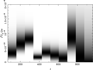
Figure 9: The maximum-likelihood CMB power spectrum derived from simulated observation of the VSA1 field. The flat band-powers were estimated in 10 spectral bins. The greyscale bars show the likelihood function evaluated along the parameter directions through the maximum-likelihood solution $\hat{\mn@boldsymbol{a}}$.

Dark areas indicate high likelihoods. The extension of the shaded areas reflects the uncertainty in the estimated parameters. As expected, the uncertainty is larger in the poorly sampled lower and higher $\ell$–bins, where the telescope sensitivity is low. On the other hand, the fairly well sampled multipoles around $\ell\approx 500$ can be determined more accurately. All reconstructed band powers are consistent with the theoretical input power spectrum. The bin width was chosen to be equal to the $1/e$-diameter of the Fourier transform of the primary beam. Thus, adjacent bins are only mildly correlated. Indeed, on calculating the curvature matrix $\mn@boldsymbol{H}(\hat{\mn@boldsymbol{a}})$ one finds that adjacent bins are anti-correlated at only the 15 per cent level.

On repeating the likelihood analysis for different realisations of the simulated noise, it is found that results are always consistent with the input spectrum and with one another. It was further verified that approximating the primary beam by a Gaussian of the same FWHM does not distort the resulting power spectrum. Moreover, the results were unaffected by ignoring the finite bandwidth of the receivers and assuming a single observing frequency in the centre of the band.

6.2 Mosaicing

We now turn to the simultaneous analysis of observations of the three fields VSA1, VSA1A and VSA1B. Since these fields overlap on the sky, the corresponding visibilities are thus correlated. The resulting likelihood function evaluated along the parameter directions through the maximum point $\hat{\mn@boldsymbol{a}}$ are plotted as the greyscale bands in Fig. 10.

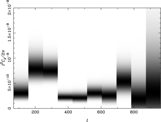
Figure 10: The maximum-likelihood CMB power spectrum derived from simulated observation of the three mosaiced fields VSA1, VSA1A and VSA1B.

Although mosaicing is often used to improve the instrumental resolution in $\ell$-space, we have chosen to compute the power spectrum in the same bins as for the single field reconstruction, in order to facilitate a direct comparison. Moreover, owing to the relatively small size of the compact VSA horns, the the aperture function is already sufficiently narrow to provide the $\ell$-resolution necessary to resolve the expected acoustic peak structure in the CMB power spectrum. As expected, the uncertainty on the flat band-powers has been significantly reduced, particularly in the poorly sampled multipole regions. Moreover, the anti-correlation between adjacent bins has reduced to around the 10 per cent level.

7 Conclusions

In this paper, we have investigated maximum-likelihood methods for estimating the power spectrum of the cosmic microwave background (CMB) from interferometer observations. In particular, we have considered the computational efficiency of several techniques for obtaining flat-band power estimates in a number of spectral bins, together with confidence limits on the power in each bin. For multifrequency data, one may also estimate the flat band-powers of Galactic foreground emission in each spectral bin. The methods developed may be applied to single-field or mosaiced observations, and take proper account of non-coplanar baselines.

The sparse nature of the covariance matrix for visibility data allows the use of sparse matrix techniques which significantly reduce the computational burden of evaluating the likelihood function, as compared with standard dense matrix routines. This enables the maximum-likelihood solution to be obtained more efficiently by numerically maximising the likelihood using only function values, as opposed to more traditional techniques, such as the Newton–Raphson algorithm, which rely on gradient and curvature information. We also find the covariance matrix of the errors on the parameters is most efficiently calculated using a numerical second-differencing approach, rather than direct calculation of the analytic expression for the curvature matrix.

The speed with which the likelihood function is calculated may be further increased by making use of the fact that only a small fraction of the total number of observed visibilities are sensitive to the flat band-power in any one spectral bin. Using this reduced data-set for each parameter enables very fast evaluation of the likelihood function along the ‘axes’ in parameter space. Indeed, we find that performing independent line-maximisations of the likelihood function along these parameter directions, and iterating until convergence, provides the computationally most efficient way of obtaining the maximum-likelihood solution.

If the spectral bins are chosen to be sufficiently wide that the flat band-powers are quasi-uncorrelated parameters, one may dispense with the Gaussian approximation to the likelihood function near its peak, and obtain (generally asymmetric) confidence intervals on each parameter by calculating the likelihood function along each parameter direction through the maximum likelihood point. This is best achieved by performing a single-to-noise eigenmode rotation for each parameter. Indeed, this method can itself be used to arrive at the maximum-likelihood solution. This is illustrated by application to simulated observations by the Very Small Array in its ‘compact’ configuration. If multifrequency data are available, this technique may also be used to marginalise over the flat band-power of foreground Galactic emission in each spectral bin.

ACKNOWLEDGMENTS

KM acknowledges support from an EU Marie Curie Fellowship.

Appendix A The general form of the visibilities covariance matrix

The contribution ${\cal S}(\mn@boldsymbol{u},\nu)$ of the sky signal to the measured visibility ${\cal V}(\mn@boldsymbol{u},\nu)$ is given simply by the convolution of the underlying Fourier modes $a(\mn@boldsymbol{u},\nu)$ with the aperture function $\tilde{A}(\mn@boldsymbol{u},\nu)$, which is itself the Fourier transform of the primary beam $A(\mn@boldsymbol{x},\nu)$ of a single antenna. Assuming that the $j$th visibility is measured at the position $\mn@boldsymbol{u}_{j}$ in the $uv$-plane and at a frequency $\nu_{j}$, we may therefore write

$${\cal S}_{j}\equiv S(\mn@boldsymbol{u}_{j},\nu_{j})=\int\!\!\!\int\!{\rm d}^{2}\mn@boldsymbol{u}\,\tilde{A}(\mn@boldsymbol{u}_{j}-\mn@boldsymbol{u},\nu_{j})a(\mn@boldsymbol{u},\nu_{j}).$$ (29)

If we write the functions $\tilde{A}(\mn@boldsymbol{u},\nu)$ and $a(\mn@boldsymbol{u},\nu)$ in terms of their real and imaginary parts,

$$\tilde{A}(\mn@boldsymbol{u},\nu)=\tilde{A}_{R}(\mn@boldsymbol{u},\nu)+i\tilde{A}_{I}(\mn@boldsymbol{u},\nu),\qquad\qquad a(\mn@boldsymbol{u},\nu)=a_{R}(\mn@boldsymbol{u},\nu)+ia_{I}(\mn@boldsymbol{u},\nu),$$

we quickly find that the real and imaginary parts of ${\cal S}_{j}$ are given by

$${\cal S}^{(R)}_{j} = \int\!\!\!\int\!{\rm d}^{2}\mn@boldsymbol{u}\,\left[\tilde{A}_{R}(\mn@boldsymbol{u}_{j}-\mn@boldsymbol{u},\nu_{j})a_{R}(\mn@boldsymbol{u},\nu_{j})-\tilde{A}_{I}(\mn@boldsymbol{u}_{j}-\mn@boldsymbol{u},\nu_{j})a_{I}(\mn@boldsymbol{u},\nu_{j})\right],$$

$${\cal S}^{(I)}_{j} = \int\!\!\!\int\!{\rm d}^{2}\mn@boldsymbol{u}\,\left[\tilde{A}_{R}(\mn@boldsymbol{u}_{j}-\mn@boldsymbol{u},\nu_{j})a_{I}(\mn@boldsymbol{u},\nu_{j})+\tilde{A}_{I}(\mn@boldsymbol{u}_{j}-\mn@boldsymbol{u},\nu_{j})a_{R}(\mn@boldsymbol{u},\nu_{j})\right].$$ (30)

We note that if the antenna function $\tilde{A}(\mn@boldsymbol{x},\nu)$ is real, then ${\cal S}_{j}^{(R)}$ depends only on the real parts $a_{R}(\mn@boldsymbol{u},\nu)$ of the underlying Fourier modes of the sky, and similarly ${\cal S}_{j}^{(I)}$ depends only on $a_{I}(\mn@boldsymbol{u},\nu)$. If the primary beam $A(\mn@boldsymbol{x},\nu)$ is real and even, then $\tilde{A}(\mn@boldsymbol{x},\nu)$ is also real and even.

The elements of the constituent submatrices of the signal covariance matrix $\mn@boldsymbol{S}$, introduced in equation (9), are most conveniently written as

$$S_{ij}^{(R,R)}\equiv\langle{\cal S}^{(R)}_{i}{\cal S}^{(R)}_{j}\rangle = {\textstyle\frac{1}{2}}[\Re(\langle{\cal S}_{i}{\cal S}_{j}^{\ast}\rangle)+\Re(\langle{\cal S}_{i}{\cal S}_{j}\rangle)],$$

$$S_{ij}^{(I,I)}\equiv\phantom{S}\langle{\cal S}^{(I)}_{i}{\cal S}^{I)}_{j}\rangle = {\textstyle\frac{1}{2}}[\Re(\langle{\cal S}_{i}{\cal S}_{j}^{\ast}\rangle)-\Re(\langle{\cal S}_{i}{\cal S}_{j}\rangle)],$$

$$S_{ij}^{(R,I)}\equiv\phantom{S}\langle{\cal S}^{(R)}_{i}{\cal S}^{I)}_{j}\rangle = {\textstyle\frac{1}{2}}[-\Im(\langle{\cal S}_{i}{\cal S}_{j}^{\ast}\rangle)+\Im(\langle{\cal S}_{i}{\cal S}_{j}\rangle)],$$

$$S_{ij}^{(I,R)}\equiv\phantom{S}\langle{\cal S}^{(I)}_{i}{\cal S}^{R)}_{j}\rangle = {\textstyle\frac{1}{2}}[\Im(\langle{\cal S}_{i}{\cal S}_{j}^{\ast}\rangle)+\Im(\langle{\cal S}_{i}{\cal S}_{j}\rangle)],$$ (31)

where $\Re$ and $\Im$ denote the real and imaginary parts of the, in general, complex quantities $\langle{\cal S}_{i}{\cal S}_{j}^{\ast}\rangle$ and $\langle{\cal S}_{i}{\cal S}_{j}\rangle$, which are given by

$$\langle{\cal S}_{i}{\cal S}_{j}^{\ast}\rangle = \int\!\!\!\int\!{\rm d}^{2}\mn@boldsymbol{u}\,\tilde{A}(\mn@boldsymbol{u}_{i}-\mn@boldsymbol{u},\nu_{i})\int\!\!\!\int\!{\rm d}^{2}\mn@boldsymbol{u}^{\prime}\,\tilde{A}^{\ast}(\mn@boldsymbol{u}_{j}-\mn@boldsymbol{u}^{\prime},\nu_{j})\langle a(\mn@boldsymbol{u},\nu_{i})a^{\ast}(\mn@boldsymbol{u}^{\prime},\nu_{j})\rangle$$

$$\langle{\cal S}_{i}{\cal S}_{j}\rangle, = \int\!\!\!\int\!{\rm d}^{2}\mn@boldsymbol{u}\,\tilde{A}(\mn@boldsymbol{u}_{i}-\mn@boldsymbol{u},\nu_{i})\int\!\!\!\int\!{\rm d}^{2}\mn@boldsymbol{u}^{\prime}\,\tilde{A}(\mn@boldsymbol{u}_{j}-\mn@boldsymbol{u}^{\prime},\nu_{j})\langle a(\mn@boldsymbol{u},\nu_{i})a(\mn@boldsymbol{u}^{\prime},\nu_{j})\rangle.$$

By definition, the matrix $\langle{\cal S}_{i}{\cal S}_{j}^{\ast}\rangle$ is Hermitian and $\langle{\cal S}_{i}{\cal S}_{j}\rangle$ is symmetric. Similarly, each of the constituent submatrices $S^{(R,R)}_{ij}$ and $S^{(I,I)}_{ij}$ is, by definition symmetric. It is also straightforward to show that $S^{(R,I)}_{ij}=S^{(I,R)}_{ji}$, so that, as expected, the full covariance matrix $\mn@boldsymbol{S}$ is symmetric. Moreover, from (30), we see that, if the aperture function $\tilde{A}(\mn@boldsymbol{u},\nu)$ is real, and the real and imaginary parts of the underlying Fourier modes $a(\mn@boldsymbol{u},\nu)$ are uncorrelated, the elements of the off-diagonal submatrices $S^{(R,I)}_{ij}$ and $S^{(I,R)}_{ij}$ are all zero. Thus, in this case, the full covariance $\mn@boldsymbol{S}$ becomes block diagonal.

If the sky emission is due to $N_{p}$ physical components, then

$$a(\mn@boldsymbol{u},\nu)=\sum_{p=1}^{N_{p}}a^{(p)}(\mn@boldsymbol{u},\nu).$$

Moreover, if we assume the spectral index of each component does not vary across the observed field, then we can describe the frequency variation of each component through the functions $f_{p}(\nu)$ $(p=1,2,\ldots,N_{p})$. In this paper, we take the reference frequency $\nu_{0}=30$ GHz and normalise the frequency dependencies so that $f_{p}(\nu_{0})=1$ for all physical components. If the emission from each physical component is statistically isotropic over the observed field and no correlations exist between the components, and using that fact that the sky is real, the Fourier modes have mean zero and their covariance properties are given by

$$\langle a^{(p)}(\mn@boldsymbol{u},\nu)[a^{(p^{\prime})}(\mn@boldsymbol{u}^{\prime},\nu^{\prime})]^{\ast}\rangle = C^{(p)}(\rho,\nu_{0})f_{p}(\nu)f_{p^{\prime}}(\nu^{\prime})\delta_{pp^{\prime}}\delta(\mn@boldsymbol{u}-\mn@boldsymbol{u}^{\prime}),$$

$$\langle a^{(p)}(\mn@boldsymbol{u},\nu)a^{(p^{\prime})}(\mn@boldsymbol{u}^{\prime},\nu^{\prime})\rangle = C^{(p)}(\rho,\nu_{0})f_{p}(\nu)f_{p^{\prime}}(\nu^{\prime})\delta_{pp^{\prime}}\delta(\mn@boldsymbol{u}+\mn@boldsymbol{u}^{\prime}),$$ (32)

where $\rho=|\mn@boldsymbol{u}|$ and $C^{(p)}(\rho,\nu_{0})$ is the ensemble-average power spectrum of the $p$th physical component at the reference frequency $\nu_{0}$. If correlations are known a priori to exist between physical components, then the expressions (32) can be straightforwardly generalised to include them. Assuming no correlations exist, however, we find that the covariance structure of the Fourier modes of the total sky emission is given by

$$\langle{\cal S}_{i}{\cal S}_{j}^{\ast}\rangle = \int\!\!\!\int\!\tilde{A}(\mn@boldsymbol{u}_{i}-\mn@boldsymbol{u},\nu_{i})\tilde{A}^{\ast}(\mn@boldsymbol{u}_{j}-\mn@boldsymbol{u},\nu_{j})\xi(|\mn@boldsymbol{u}|,\nu_{i},\nu_{j})~{}{\rm d}^{2}\mn@boldsymbol{u},$$ (33)

$$\langle{\cal S}_{i}{\cal S}_{j}\rangle = \int\!\!\!\int\!\tilde{A}(\mn@boldsymbol{u}_{i}-\mn@boldsymbol{u},\nu_{i})\tilde{A}(\mn@boldsymbol{u}_{j}+\mn@boldsymbol{u},\nu_{j})\xi(|\mn@boldsymbol{u}|,\nu_{i},\nu_{j})~{}{\rm d}^{2}\mn@boldsymbol{u},$$ (34)

where we have introduced the generalised power spectrum $\xi(\rho,\nu_{i},\nu_{j})$, which is defined by

$$\xi(\rho,\nu_{i},\nu_{j})=\sum_{p=1}^{N_{p}}f_{p}(\nu_{i})f_{p}(\nu_{j})C^{(p)}(\rho,\nu_{0}).$$ (35)

We note, in particular, that if the aperture function satisfies $\tilde{A}^{\ast}(\mn@boldsymbol{u},\nu)=\tilde{A}(-\mn@boldsymbol{u},\nu)$, which corresponds to a real primary beam $A(\mn@boldsymbol{x},\nu)$, then

$$\langle{\cal S}(\mn@boldsymbol{u}_{i},\nu_{i}){\cal S}_{j}(\mn@boldsymbol{u}_{j},\nu_{j})\rangle=\langle{\cal S}(\mn@boldsymbol{u}_{i},\nu_{i}){\cal S}_{j}^{\ast}(-\mn@boldsymbol{u}_{j},\nu_{j})\rangle.$$ (36)

Thus, in this case, one need only evaluate $\langle{\cal S}_{i}{\cal S}_{j}\rangle$ and use the result (36) in order to construct the full signal covariance matrix $\mn@boldsymbol{S}$, whose elements are defined in (31).

If we introduce polar coordinates $(\rho,\theta)$ into the $uv$-plane, we can write (33) and (34) formally as the one-dimensional integrals

$$\langle{\cal S}_{i}{\cal S}_{j}^{\ast}\rangle = \int_{0}^{\infty}{\rm d}\rho\,\rho\,W^{(1)}_{ij}(\rho)\,\xi(\rho,\nu_{i},\nu_{j}),$$

$$\langle{\cal S}_{i}{\cal S}_{j}\rangle = \int_{0}^{\infty}{\rm d}\rho\,\rho\,W^{(2)}_{ij}(\rho)\,\xi(\rho,\nu_{i},\nu_{j}),$$ (37)

where the window functions $W^{(1)}_{ij}(\rho)$ and $W^{(2)}_{ij}(\rho)$ are defined respectively by

$$W^{(1)}_{ij}(\rho) = \int_{0}^{2\pi}{\rm d}\theta\,\tilde{A}(\mn@boldsymbol{u}_{i}-\mn@boldsymbol{u},\nu_{i})\tilde{A}^{\ast}(\mn@boldsymbol{u}_{j}-\mn@boldsymbol{u},\nu_{j}),$$ (38)

$$W^{(2)}_{ij}(\rho) = \int_{0}^{2\pi}{\rm d}\theta\,\tilde{A}(\mn@boldsymbol{u}_{i}-\mn@boldsymbol{u},\nu_{i})\tilde{A}(\mn@boldsymbol{u}_{j}+\mn@boldsymbol{u},\nu_{j}),$$ (39)

and $\mn@boldsymbol{u}=\rho(\cos\theta,\sin\theta)^{\rm t}$. In the case where $\tilde{A}^{*}(\mn@boldsymbol{u},\nu)=\tilde{A}(-\mn@boldsymbol{u},\nu)$, one need only evaluate $W^{(1)}_{ij}(\rho)$ and use (36) and (31) to construct $\mn@boldsymbol{S}$.

Appendix B Mosaicing

For mosaiced observations, the pointing centres of individual observations are not identical with the global phase–tracking centre. This can be accommodated by shifting the primary beam response pattern $A(\mn@boldsymbol{x},\nu)$ to the corresponding pointing centre. Thus, let us assume that the $j$th visibility is measured at the position $\mn@boldsymbol{u}_{j}$ in the $uv$-plane, at an observing frequency $\nu_{j}$, and is referred to the pointing centre $\mn@boldsymbol{x}_{j}$. In this case, the expression corresponding to (3) becomes

$${\cal S}_{j}\equiv{\cal S}(\mn@boldsymbol{u}_{j},\nu_{j}) = \int\!\!\!\int\!A(\mn@boldsymbol{x}-\mn@boldsymbol{x}_{j},\nu_{j})\frac{\Delta T(\mn@boldsymbol{x},\nu_{j})}{T}e^{2\pi i\mn@boldsymbol{u}_{j}\cdot\mn@boldsymbol{x}}~{}{\rm d}^{2}\mn@boldsymbol{x}$$ (40)

$$= \int\!\!\!\int\!\tilde{A}(\mn@boldsymbol{u}_{j}-\mn@boldsymbol{u},\nu_{j})e^{2\pi i(\mn@boldsymbol{u}_{j}-\mn@boldsymbol{u})\cdot\mn@boldsymbol{x}_{j}}a(\mn@boldsymbol{u},\nu_{j})~{}{\rm d}^{2}\mn@boldsymbol{u},$$

where the second equality follows from the Fourier shift theorem. This illustrates that the effect of mosaicing is simply to introduce a phase shift, so that the effective aperture function for the $j$th field becomes

$$\tilde{A}_{\rm eff}(\mn@boldsymbol{u},\nu_{j})=\tilde{A}(\mn@boldsymbol{u},\nu_{j})\ e^{2\pi i\mn@boldsymbol{u}\cdot\mn@boldsymbol{x}_{j}},$$ (41)

which is, in general, complex. The covariance properties of the visibilities may then be obtained straightforwardly from the expressions given in Appendix A, by replacing $\tilde{A}(\mn@boldsymbol{u},\nu)$ with $\tilde{A}_{\rm eff}(\mn@boldsymbol{u},\nu)$ given in (41). In this case, however, the corresponding window functions (38) and (39) will also be functions of $\mn@boldsymbol{x}_{i}$ and $\mn@boldsymbol{x}_{j}$. In particular, we find

$$W^{(1)}_{ij}(\rho) = e^{2\pi i(\mn@boldsymbol{u}_{i}\cdot\mn@boldsymbol{x}_{i}-\mn@boldsymbol{u}_{j}\cdot\mn@boldsymbol{x}_{j})}\int_{0}^{2\pi}{\rm d}\theta\,\tilde{A}(\mn@boldsymbol{u}_{i}-\mn@boldsymbol{u},\nu_{i})\tilde{A}^{\ast}(\mn@boldsymbol{u}_{j}-\mn@boldsymbol{u},\nu_{j})e^{2\pi i\mn@boldsymbol{u}\cdot(\mn@boldsymbol{x}_{j}-\mn@boldsymbol{x}_{i})},$$

$$W^{(2)}_{ij}(\rho) = e^{2\pi i(\mn@boldsymbol{u}_{i}\cdot\mn@boldsymbol{x}_{i}+\mn@boldsymbol{u}_{j}\cdot\mn@boldsymbol{x}_{j})}\int_{0}^{2\pi}{\rm d}\theta\,\tilde{A}(\mn@boldsymbol{u}_{i}-\mn@boldsymbol{u},\nu_{i})\tilde{A}(\mn@boldsymbol{u}_{j}+\mn@boldsymbol{u},\nu_{j})e^{2\pi i\mn@boldsymbol{u}\cdot(\mn@boldsymbol{x}_{j}-\mn@boldsymbol{x}_{i})}.$$ (42)

We note that, if the primary beam ${A}(\mn@boldsymbol{x},\nu)$ is real, then the effective aperture function (41) still satisfies $\tilde{A}^{\ast}_{\rm eff}(\mn@boldsymbol{u},\nu)=\tilde{A}_{\rm eff}(-\mn@boldsymbol{u},\nu)$. Thus, (36) remains valid and one need only evaluate $\langle{\cal S}_{i}{\cal S}_{j}^{\ast}\rangle$ (and hence $W^{(1)}_{ij}(\rho)$) to construct $\mn@boldsymbol{S}$.

Although the above description of mosaicing is straightforward, additional subtleties exist in practice, since interferometers such as the VSA do not refer the phases of all visibilities to the same constant phase-tracking centre. Instead, the phases of visibilities are referred to the pointing centre of the corresponding field. In this case, the visibilities are given by

$${\cal S}_{j}\equiv{\cal S}(\mn@boldsymbol{u}_{j},\nu_{j}) = \int\!\!\!\int\!A(\mn@boldsymbol{x},\nu_{j})\frac{\Delta T(\mn@boldsymbol{x}+\mn@boldsymbol{x}_{j},\nu_{j})}{T}e^{2\pi i\mn@boldsymbol{u}_{j}\cdot\mn@boldsymbol{x}}~{}{\rm d}^{2}\mn@boldsymbol{x}$$ (43)

$$= \int\!\!\!\int\!A(\mn@boldsymbol{x}-\mn@boldsymbol{x}_{j},\nu_{j})\frac{\Delta T(\mn@boldsymbol{x},\nu_{j})}{T}e^{-2\pi i\mn@boldsymbol{u}_{j}\cdot\mn@boldsymbol{x}_{j}}e^{2\pi i\mn@boldsymbol{u}_{j}\cdot\mn@boldsymbol{x}}~{}{\rm d}^{2}\mn@boldsymbol{x}$$

$$= \int\!\!\!\int\!\tilde{A}(\mn@boldsymbol{u}_{j}-\mn@boldsymbol{u},\nu_{j})a(\mn@boldsymbol{u},\nu_{j})e^{-2\pi i\mn@boldsymbol{u}\cdot\mn@boldsymbol{x}_{j}}~{}{\rm d}^{2}\mn@boldsymbol{u}.$$

We note that (40) and (43) differ only by a phase shift $\exp[-2\pi i\mn@boldsymbol{u}_{j}\cdot\mn@boldsymbol{x}_{j}]$. However, the vectors $\mn@boldsymbol{u}_{j}$ are given in different coordinate systems, referring in each case to the corresponding phase–tracking centre. From (43), we see that we may obtain the covariance properties of the corresponding visibilities from the equations given in Appendix A, provided we replace $\tilde{A}(\mn@boldsymbol{u},\nu_{j})$ by the new effective aperture function for the $j$th field, which is given by

$$\tilde{A}_{\rm eff}(\mn@boldsymbol{u},\nu_{j})=\tilde{A}(\mn@boldsymbol{u},\nu_{j})\ e^{2\pi i(\mn@boldsymbol{u}-\mn@boldsymbol{u}_{j})\cdot\mn@boldsymbol{x}_{j}},$$ (44)

and similarly for the $i$ term. Hence, in this case, the window functions are given by

$$W^{(1)}_{ij}(\rho) = \int_{0}^{2\pi}{\rm d}\theta\,\tilde{A}(\mn@boldsymbol{u}_{i}-\mn@boldsymbol{u},\nu_{i})\tilde{A}^{\ast}(\mn@boldsymbol{u}_{j}-\mn@boldsymbol{u},\nu_{j})e^{2\pi i\mn@boldsymbol{u}\cdot(\mn@boldsymbol{x}_{j}-\mn@boldsymbol{x}_{i})},$$

$$W^{(2)}_{ij}(\rho) = \int_{0}^{2\pi}{\rm d}\theta\,\tilde{A}(\mn@boldsymbol{u}_{i}-\mn@boldsymbol{u},\nu_{i})\tilde{A}(\mn@boldsymbol{u}_{j}+\mn@boldsymbol{u},\nu_{j})e^{2\pi i\mn@boldsymbol{u}\cdot(\mn@boldsymbol{x}_{j}-\mn@boldsymbol{x}_{i})},$$ (45)

We note that, for a real primary beam, the relation (36) again holds, so that only $\langle{\cal S}_{i}{\cal S}_{j}^{\ast}\rangle$ (and hence $W^{(1)}_{ij}(\rho)$) need be calculated in order to construct $\mn@boldsymbol{S}$.

Appendix C Large fields and non–coplanar baselines

In Appendices A and B, we have assumed that the field of view of the telescope is small enough that the $w$-distortions discussed in section 2.4 can be neglected. Without the assumption of a small field size or vanishing $w$-components of the baselines, the contribution of the sky signal to a measured visibility is given by (e.g. Thompson et al. 1994)

$${\cal S}\equiv{\cal S}(\mn@boldsymbol{u}_{j},w_{j},\nu_{j})=\int\!\!\!\int\!{\rm d}^{2}\mn@boldsymbol{x}\,A(\mn@boldsymbol{x},\nu_{j})\frac{\Delta T}{T}(\mn@boldsymbol{x},\nu_{j})e^{2\pi i(\mn@boldsymbol{u}_{j}\cdot\mn@boldsymbol{x}+w_{j}(\sqrt{1-|\mn@boldsymbol{x}|^{2}}-1))}\frac{1}{\sqrt{1-|\mn@boldsymbol{x}|^{2}}},$$ (46)

where $w_{j}$ is the component of the baseline in the direction of the phase–tracking centre. For convenience, we assume that pointing and phase-tracking centres are identical. The factor $\sqrt{1-|\mn@boldsymbol{x}|^{2}}-1\approx-\frac{1}{2}|\mn@boldsymbol{x}|^{2}$ is small (for example, $\frac{1}{2}|\mn@boldsymbol{x}|^{2}<0.001$ at an angle of $x=2.3\degr$). We can thus either omit the factor ${1}/{\sqrt{1-|\mn@boldsymbol{x}|^{2}}}\approx 1$ or absorb it into the definition of the primary beam $A(\mn@boldsymbol{x},\nu)$. We obtain

$${\cal S}(\mn@boldsymbol{u}_{j},w_{j},\nu_{j})=\int\!\!\!\int\!{\rm d}^{2}\mn@boldsymbol{x}\,A(\mn@boldsymbol{x},\nu_{j})e^{-\pi iw_{j}|\mn@boldsymbol{x}|^{2}}\frac{\Delta T}{T}(\mn@boldsymbol{x},\nu_{j})e^{2\pi i\mn@boldsymbol{u}_{j}\cdot\mn@boldsymbol{x}}.$$ (47)

Defining an effective beam

$$A_{\rm eff}(\mn@boldsymbol{x},w,\nu_{j})=A(\mn@boldsymbol{x},\nu_{j})\exp(-\pi iw|\mn@boldsymbol{x}|^{2}),$$ (48)

the visibilities are

$${\cal S}_{j}={\cal S}(\mn@boldsymbol{u}_{j},w_{j},\nu_{j})=\int\!\!\!\int\!{\rm d}^{2}\mn@boldsymbol{u}\,\tilde{A}_{\rm eff}(\mn@boldsymbol{u}_{j}-\mn@boldsymbol{u},w_{j},\nu_{j})a(\mn@boldsymbol{u},\nu_{j}),$$ (49)

where the Fourier transform of $A_{\rm eff}$ is given by a convolution

$$\tilde{A}_{\rm eff}(\mn@boldsymbol{u},w,\nu)=\int\!\!\!\int\!{\rm d}^{2}\mn@boldsymbol{u}^{\prime}\,\tilde{A}(\mn@boldsymbol{u}-\mn@boldsymbol{u}^{\prime},\nu)\frac{1}{iw}e^{i\pi|\mn@boldsymbol{u}^{\prime}|^{2}/w}.$$ (50)

The covariance structure of the visibilities can then by found by using this expression in place of $\tilde{A}(\mn@boldsymbol{u},\nu)$ in the results of Appendix A. In particular, we note that if $\tilde{A}_{\rm eff}(\mn@boldsymbol{u}_{i}+\mn@boldsymbol{u},w_{i},\nu_{i})=\tilde{A}_{\rm eff}^{\ast}((-\mn@boldsymbol{u}_{i})-\mn@boldsymbol{u},-w_{i},\nu_{i})$, we find

$$\langle{\cal S}(\mn@boldsymbol{u}_{i},w_{i},\nu_{i}){\cal S}(\mn@boldsymbol{u}_{j},w_{j},\nu_{j})\rangle=\langle{\cal S}(\mn@boldsymbol{u}_{i},w_{i},\nu_{i}){\cal S}^{\ast}(-\mn@boldsymbol{u}_{j},-w_{j},\nu_{j})\rangle.$$ (51)

Thus, in this case, the full signal covariance $\mn@boldsymbol{S}$ can be obtained from (33) and (31).

Appendix D Gaussian primary beam

Let us denote the primary beam at the $i$th observing frequency $\nu_{i}$ by $A(\mn@boldsymbol{x},\nu_{i})=\exp(-|\mn@boldsymbol{x}|^{2}/2\sigma_{i}^{2})$, where $\sigma_{i}$ is the dispersion of the primary beam at this frequency. The aperture function is simply the Fourier transform of the primary beam, and is given by $\tilde{A}(\mn@boldsymbol{u},\nu_{i})=2\pi\sigma_{i}^{2}\exp(-2\pi^{2}\sigma_{i}^{2}|\mn@boldsymbol{u}|^{2})$. As we now show, in this case it is possible to obtain analytical formulae for the window functions $W^{(1)}_{ij}(\rho)$ and $W^{(2)}_{ij}(\rho)$.

D.1 Two-dimensional approximation

We begin by considering the general case of mosaiced observations, but in the approximation that the visibilities can be obtained by a two-dimensional Fourier transformation of the sky brightness distribution and the primary beam. In that case, from (45), we have

$$W^{(1)}_{ij}(\rho)=(2\pi\sigma_{i}\sigma_{j})^{2}\int\!\!\!\int\!{\rm d}^{2}\mn@boldsymbol{u}\,\exp(-2\pi^{2}\sigma_{i}^{2}|\mn@boldsymbol{u}_{i}-\mn@boldsymbol{u}|^{2})\exp(-2\pi^{2}\sigma_{j}^{2}|\mn@boldsymbol{u}_{j}-\mn@boldsymbol{u}|^{2})\exp(2\pi i\mn@boldsymbol{u}\cdot(\mn@boldsymbol{x}_{j}-\mn@boldsymbol{x}_{i})),$$ (52)

where all visibilities are referred to the pointing centre of the corresponding field as in (45). If we introduce the vectors

$$\mn@boldsymbol{q}=\sigma_{i}^{2}\mn@boldsymbol{u}_{i}+\sigma_{j}^{2}\mn@boldsymbol{u}_{j},\quad\mn@boldsymbol{x}=\mn@boldsymbol{x}_{j}-\mn@boldsymbol{x}_{i}$$ (53)

and use $\theta$ to denote the angle between $\mn@boldsymbol{q}$ and the position vector $\mn@boldsymbol{u}$ in the Fourier plane, and $\phi$ the angle between $\mn@boldsymbol{x}$ and $\mn@boldsymbol{q}$, we find that the window function can be written as

$$W^{1}_{ij}(\rho)=(2\pi\sigma_{i}\sigma_{j})^{2}\exp[-2\pi^{2}(\sigma^{2}_{i}|\mn@boldsymbol{u}_{i}|^{2}+\sigma^{2}_{j}|\mn@boldsymbol{u}_{j}|^{2})]\exp[-2\pi^{2}(\sigma_{i}^{2}+\sigma_{j}^{2})\rho^{2}]\int_{0}^{2\pi}\!{\rm d}\theta\,\exp[4\pi^{2}|\mn@boldsymbol{q}|\rho\cos\theta]\exp[2\pi i|\mn@boldsymbol{x}|\rho\cos(\theta+\phi)].$$

The integral on $\theta$ can be written as

$$J_{ij}(\rho)=\int_{0}^{2\pi}\!{\rm d}\theta\,\exp[4\pi^{2}|\mn@boldsymbol{q}|\rho\cos\theta]\exp[2\pi i|\mn@boldsymbol{x}|\rho(\cos\theta\cos\phi-\sin\theta\sin\phi)]=\int_{0}^{2\pi}\!{\rm d}\theta\,\exp[p\cos\theta]\exp[ia\cos\theta+ib\sin\theta],$$ (54)

where $p=4\pi^{2}|\mn@boldsymbol{q}|\rho$, $a=2\pi|\mn@boldsymbol{x}|\rho\cos\phi$ and $b=-2\pi|\mn@boldsymbol{x}|\rho\sin\phi$ (compare Gradshteyn & Ryzhik, integrals 3.937). Substituting $z=\exp(i\theta)$, ${\rm d}z=iz\,d\theta$, $\cos\theta=(z+z^{-1})/2$ and $\sin\theta=(z-z^{-1})/(2i)$, we find

$$J_{ij}(\rho)=\oint_{\cal C}\!{\rm d}z\,\frac{1}{iz}\exp\left[(p+ia)\frac{z+z^{-1}}{2}+ib\frac{z-z^{-1}}{2i}\right]=\oint_{\cal C}\!{\rm d}z\,\frac{1}{iz}\exp\left[(p+b+ia)\frac{z}{2}+(p-b+ia)\frac{z^{-1}}{2}\right],$$

where the curve ${\cal C}$ is the unit circle in the complex plane. Defining $f(z)=z^{-1}\exp[Az+Bz^{-1}]$, where $A=(p+b+ia)/2$ and $B=(p-b+ia)/2$, we obtain

$$J_{ij}(\rho)=\oint_{\cal C}\!{\rm d}z\,\frac{1}{i}f(z)=2\pi\mbox{Res}(f,0),$$

where $\mbox{Res}(f,0)$ denotes the residue of $f(z)$ around the essential singularity $z=0$. The Laurent series of $f$ about this point has the form $f(z)=\sum_{m=-\infty}^{\infty}c_{m}(z-0)^{m}$ and is given by

$$f(z) = \frac{1}{z}\exp[Az+Bz^{-1}]=\frac{1}{z}\sum_{m=0}^{\infty}\frac{(Az+Bz^{-1})^{m}}{m!}$$

$$= \frac{1}{z}\sum_{m=0}^{\infty}\sum_{n=0}^{m}\frac{1}{m!}{{}^{m}}C_{n}A^{n}B^{m-n}z^{2n-m}=\sum_{m=0}^{\infty}\sum_{n=0}^{m}\frac{1}{n!(m-n)!}A^{n}B^{m-n}z^{2n-m-1},$$

from which we can read off

$$\mbox{Res}(f,0)=c_{-1}=\sum_{n=0}^{\infty}\frac{(AB)^{n}}{(n!)^{2}}=\sum_{n=0}^{\infty}\frac{(\frac{1}{2}\sqrt{4AB})^{2n}}{(n!)^{2}}=I_{0}(\sqrt{4AB}),$$

where $I_{0}(z)=\sum_{n=0}^{\infty}(\frac{1}{2}z)^{2n}/(n!)^{2}$ is the modified Bessel function of the first kind and order zero for a complex argument $z$. Substituting all the abbreviations, we have

$$4AB=p^{2}-a^{2}-b^{2}+2iap=[(2\pi\rho)^{2}[(2\pi|\mn@boldsymbol{q}|)^{2}-|\mn@boldsymbol{x}|^{2}+i(4\pi\mn@boldsymbol{q}\cdot\mn@boldsymbol{x})].$$ (55)

Thus, the window function is given by the (complex) analytical expression

$$W^{(1)}_{ij}(\rho)=(2\pi)^{3}(\sigma_{i}\sigma_{j})^{2}\exp[-2\pi^{2}(\sigma^{2}_{i}|\mn@boldsymbol{u}_{i}|^{2}+\sigma^{2}_{j}|\mn@boldsymbol{u}_{j}|^{2})]\exp[-2\pi^{2}(\sigma_{i}^{2}+\sigma_{j}^{2})\rho^{2}]I_{0}(2\pi\sqrt{k}\rho),$$ (56)

where

$$k=(2\pi|\mn@boldsymbol{q}|)^{2}-|\mn@boldsymbol{x}|^{2}+i(4\pi\mn@boldsymbol{q}\cdot\mn@boldsymbol{x}).$$ (57)

The full signal covariance matrix $\mn@boldsymbol{S}$ can then be derived using (37) and (31).

A useful check of our result (56) is provided by the special case of a single field, for which $\mn@boldsymbol{x}_{i}=\mn@boldsymbol{x}_{j}$, and so $\mn@boldsymbol{x}=\mn@boldsymbol{x}_{j}-\mn@boldsymbol{x}_{i}=\mn@boldsymbol{0}$. Thus, $J_{ij}(\rho)$ is given by the real integral

$$J_{ij}(\rho)=\int_{0}^{2\pi}\!{\rm d}\theta\,\exp[4\pi^{2}|\mn@boldsymbol{q}|\rho\cos\theta]=\int_{0}^{2\pi}\!{\rm d}\theta\,\exp[4\pi^{2}|\mn@boldsymbol{q}|\rho\sin\theta]=2\pi I_{0}(4\pi^{2}|\mn@boldsymbol{q}|\rho).$$

Therefore, in this case, the elements of the window function are given by the real expression

$$W^{(1)}_{ij}(\rho)=(2\pi)^{3}(\sigma_{i}\sigma_{j})^{2}\exp[-2\pi^{2}(\sigma^{2}_{i}|\mn@boldsymbol{u}_{i}|^{2}+\sigma^{2}_{j}|\mn@boldsymbol{u}_{j}|^{2})]\exp[-2\pi^{2}(\sigma_{i}^{2}+\sigma_{j}^{2})\rho^{2}]I_{0}(4\pi^{2}|\sigma_{i}^{2}\mn@boldsymbol{u}_{i}+\sigma_{j}^{2}\mn@boldsymbol{u}_{j}|\rho),$$

which is identical to setting $\mn@boldsymbol{x}=\mn@boldsymbol{0}$ in (57). Comparison with (31) shows that the offdiagonal blocks $S_{ij}^{(I,R)}$ and $S_{ij}^{(R,I)}$ of the signal covariance matrix vanish and real and imaginary parts of the visibilities can be treated independently.

D.2 Non-coplanar baselines and the $w$-correction

We now consider the effects of non-vanishing $w$-components on our expression (56) for the window function $W^{(1)}_{ij}$. From (48), for a Gaussian primary beam of width $\sigma$, the effective primary beam is given by $A_{\rm eff}(\mn@boldsymbol{x},w,\nu)=\exp(-|\mn@boldsymbol{x}|^{2}(\frac{1}{2\sigma^{2}}+i\pi w))$. On Fourier transforming, we obtain the effective aperture function

$$\tilde{A}_{\rm eff}(\mn@boldsymbol{u},w,\nu)=2\pi\sigma^{2}\frac{1-i\phi}{1+\phi^{2}}e^{-2\pi^{2}\sigma^{2}\frac{1-i\phi}{1+\phi^{2}}|\mn@boldsymbol{u}|^{2}}=2\pi\hat{\sigma}^{2}(1-i\phi)e^{-2\pi^{2}\hat{\sigma}^{2}(1-i\phi)|\mn@boldsymbol{u}|^{2}},$$

where $\phi=2\pi\sigma^{2}w$ and $\hat{\sigma}^{2}=\sigma^{2}/(1+\phi^{2})=\sigma^{2}/(1+4\pi^{2}\sigma^{4}w^{2})$.

We see that the effect of the $w$–distortion can be considered as turning the primary beam into a complex Gaussian, whose Fourier transform is again a complex Gaussian. This can easily be taken into account in the analysis from section D.1 by replacing

$$\sigma^{2}\rightarrow\sigma^{2}\frac{1-i\phi}{1+\phi^{2}}=\hat{\sigma}^{2}(1-i\phi)$$

in (52). For the angular integration (54), we then have to use the vectors

$$\mn@boldsymbol{q}=\hat{\sigma}_{i}^{2}\mn@boldsymbol{u}_{i}+\hat{\sigma}_{j}^{2}\mn@boldsymbol{u}_{j},\quad\mn@boldsymbol{x}=\mn@boldsymbol{x}_{j}-\mn@boldsymbol{x}_{i}+2\pi\left(\phi_{j}\hat{\sigma}_{j}^{2}\mn@boldsymbol{u}_{j}-\phi_{i}\hat{\sigma}_{i}^{2}\mn@boldsymbol{u}_{i}\right)$$ (58)

instead of (53). The final expression for the window function $W^{(1)}_{ij}(\rho)$ is

$$W^{(1)}_{ij}(\rho) = (2\pi)^{3}(\hat{\sigma}_{i}\hat{\sigma}_{j})^{2}(1+\phi_{i}\phi_{j}+i(\phi_{j}-\phi_{i}))\ e^{-2\pi^{2}(\hat{\sigma}^{2}_{i}|\mn@boldsymbol{u}_{i}|^{2}+\hat{\sigma}^{2}_{j}|\mn@boldsymbol{u}_{j}|^{2})}\ e^{-2\pi^{2}i(\phi_{j}\hat{\sigma}^{2}_{j}|\mn@boldsymbol{u}_{j}|^{2}-\phi_{i}\hat{\sigma}^{2}_{i}|\mn@boldsymbol{u}_{i}|^{2})}$$

$$\times\ e^{-2\pi^{2}(\hat{\sigma}_{i}^{2}+\hat{\sigma}_{j}^{2})\rho^{2}}\ e^{-2\pi^{2}i(\phi_{j}\hat{\sigma}_{j}^{2}-\phi_{i}\hat{\sigma}_{i}^{2})\rho^{2}}I_{0}(2\pi\sqrt{k}\rho),$$

where now $k=(2\pi|\mn@boldsymbol{q}|)^{2}-|\mn@boldsymbol{x}|^{2}+i(4\pi\mn@boldsymbol{q}\cdot\mn@boldsymbol{x})$ as in (57), but with $\mn@boldsymbol{q}$ and $\mn@boldsymbol{x}$ defined in (58), and $\hat{\sigma}_{i}=\sigma_{i}/(1+\phi_{i}^{2})$ with $\phi_{i}=2\pi\sigma^{2}_{i}w_{i}$. Furthermore, we note that, $\tilde{A}_{\rm eff}(\mn@boldsymbol{u}_{i}+\mn@boldsymbol{u},w_{i},\nu_{i})=\tilde{A}_{\rm eff}^{\ast}((-\mn@boldsymbol{u}_{i})-\mn@boldsymbol{u},-w_{i},\nu_{i})$, and so (51) is satisfied. Thus, the full signal covariance $\mn@boldsymbol{S}$ can be obtained from (51) and (31).

Appendix E Signal-to-noise eigenmodes

As discussed in section 5.3.2, it is useful to calculate the log-likelihood function along each coordinate direction in parameter space. In other words, one wishes to calculate the log-likelihood as a function of a single parameter $a_{k}$, while the remaining parameters are kept fixed; we denote this by $\ln{\cal L}(\mn@boldsymbol{v}|a_{k})$. In fact, as shown in section 5.3, for interferometer data one may replace the full data vector, $\mn@boldsymbol{v}$, with a reduced data vector $\tilde{\mn@boldsymbol{v}}_{k}$ that contains only those visibilities sensitive to changes in the flat band-power $a_{k}$. Hence, for various values of $a_{k}$, one must evaluate

$$\ln{\cal L}(\tilde{\mn@boldsymbol{v}}_{k}|a_{k})=\mbox{constant}-{\textstyle\frac{1}{2}}\left[\ln|\mn@boldsymbol{C}(\mn@boldsymbol{a})|+\tilde{\mn@boldsymbol{v}}_{k}^{\rm t}\mn@boldsymbol{C}^{-1}(\mn@boldsymbol{a})\tilde{\mn@boldsymbol{v}}_{k}\right].$$

This calculation is neatly performed by using the method of signal-to-noise eigenmodes, which are a special case of Karhunen-Loeve modes, where the parameter dependence is linear (affine) (Bond 1995; Bond, Jaffe & Knox 1998; Tegmark, Taylor & Heavens 1997).

The covariance matrix $\mn@boldsymbol{C}(\mn@boldsymbol{a})=\mn@boldsymbol{S}(\mn@boldsymbol{a})+\mn@boldsymbol{N}$ contains contributions from the sky signal and the noise. Since the parameters are flat band-powers in spectral bins, we can write the signal contribution as

$$\mn@boldsymbol{S}(\mn@boldsymbol{a})=\mn@boldsymbol{S}_{1}(a_{k})+\mn@boldsymbol{S}_{2}(\check{\mn@boldsymbol{a}}),$$

where $\check{\mn@boldsymbol{a}}$ denotes collectively the fixed parameters $a_{k^{\prime}}$ $(k^{\prime}\neq k)$. Hence, $\mn@boldsymbol{S}_{1}$ depends only on the parameter of interest and $\mn@boldsymbol{S}_{2}$ depends only on the (fixed) values of the other parameters, and is hence a fixed matrix. Moreover, the matrix $\mn@boldsymbol{S}_{1}$ is linear in $a_{k}$, since it is simply a flat band-power, and so we may write $\mn@boldsymbol{S}_{1}(a_{k})=a_{k}\mn@boldsymbol{U}$, where the fixed matrix $\mn@boldsymbol{U}=\mn@boldsymbol{S}_{1}(1)$. Thus the total covariance matrix can be written as

$$\mn@boldsymbol{C}(\mn@boldsymbol{a})=a_{k}\mn@boldsymbol{U}+\mn@boldsymbol{S}_{2}(\check{\mn@boldsymbol{a}})+\mn@boldsymbol{N}\equiv a_{k}\mn@boldsymbol{U}+\mn@boldsymbol{V},$$

where $\mn@boldsymbol{U}$ is the fixed ‘unit signal’ covariance matrix and $\mn@boldsymbol{V}$ is the fixed ‘generalised noise’ matrix.

Since $\mn@boldsymbol{U}$ and $\mn@boldsymbol{V}$ are both real symmetric matrices, they can be diagonalised simultaneously by a single similarity transformation. This is most easily achieved by solving the generalised eigenproblem

$$\mn@boldsymbol{Ux}=\lambda\mn@boldsymbol{Vx}.$$

Let us denote the corresponding eigenvalues by $\lambda_{i}$ and the eigenvectors by $\mn@boldsymbol{e}_{i}$, which are normalised such that $\mn@boldsymbol{e}_{i}^{\rm t}\mn@boldsymbol{V}\mn@boldsymbol{e}_{i}=1$. If we now define a new set of ‘rotated’ data by $\zeta_{i}=\mn@boldsymbol{e}_{i}\cdot\tilde{v}_{k}$, then it is straightforward to show that these new variables are uncorrelated for any value of the parameter $a_{k}$, and have a covariance matrix with elements

$$\langle\zeta_{i}\zeta_{j}\rangle=(1+a_{k}\lambda_{i})\delta_{ij}.$$ (59)

The $\zeta_{i}$ called the signal-to-noise eigenmodes, and each is a linear combination of the original data items. Modes corresponding to a large eigenvalue are expected to be well-determined, while modes with small eigenvalues are poorly-determined and do not contribute significantly to the value of the likelihood function.

From (59), we see that the log-likelihood, as a function of the parameter $a_{k}$ (with the others held fixed) is given simply by

$$\ln{\cal L}(\mn@boldsymbol{\zeta}|a_{k})=\mbox{constant}-{\textstyle\frac{1}{2}}\sum_{i}\left[\ln(1+a_{k}\lambda_{i})+\frac{\zeta_{i}^{2}}{1+a_{k}\lambda_{i}}\right].$$

This is trivial to evaluate and so the log-likelihood function can be calculated at a large number of points along in $a_{k}$-direction at virtually no extra computational cost.

References

- [Anderson et al. 1999] Anderson E. et al., 1999, LAPACK Users’ Guide, 3rd ed. SIAM, Philadelphia
- [Baker et al. 1999] Baker J.C. et al., 1999, MNRAS, 308, 1173
- [Bond 1995] Bond J.R., 1995, Phys. Rev. Lett., 74, 4369
- [Bond et al. 1998] Bond J.R., Jaffe A.H., Knox L., 1998, Phys. Rev. D, 57, 2117
- [Bond et al. 2000] Bond J.R., Jaffe A.H., Knox L., 2000, ApJ, 2000, 533, 19
- [Borrill 1999] Borrill J., 1999, Proceedings of the 5th European SGI/Cray MPP Workshop, astro-ph/9911389
- [Cornwell 1988] Cornwell T.J., 1988, A&A, 202, 316
- [Cornwell & Perley 1992] Cornwell T.J., Perley R.A., 1992, A&A, 261, 353
- [Cornwell et al. 1993] Cornwell T.J., Holdaway M.A., Uson J.M., 1993, A&A, 271, 697
- [Christensen et al. 2001] Christensen N., Meyer R., Knox L., Luey B., 2001, Classical and Quantum Gravity, 18, 2677
- [Eaton 1983] Eaton M.L., 1983, Multivariate Statistics. Wiley, New York
- [Ekers & Rots 1979] Ekers R.D., Rots A.H., 1979, in van Schooneveld C., ed., ASSL Vol. 76: IAU Colloq. 49: Image Formation from Coherence Functions in Astronomy. C.D. Reidel Publishing Co., p. 61
- [Gradshteyn & Ryzhik 1994] Gradstheyn I.S., Ryzhik I.M., 1994, Table of Integrals, Series and Products, 5th edition, Alan Jeffrey ed. Academic Press
- [Greenbaum 1997] Greenbaum A., 1997, Iterative Methods for Solving Linear Systems. SIAM, Philadelphia
- [Halverson et al. 2001] Halverson N.W. et al., 2001, astro-ph/0104489
- [Hobson et al. 1995] Hobson M.P., Lasenby A.N., Jones M.E., 1995, MNRAS, 275, 863
- [Hobson & Magueijo 1996] Hobson M.P., Magueijo J., 1996, MNRAS, 283, 1133
- [Holdaway 1999] Holdaway M.A., 1999, in ASP Conf. Ser. 180: Synthesis Imaging in Radio Astronomy II, p. 401
- [Jones 1990] Jones M.E., 1990, Ph.D. Thesis, University of Cambridge
- [Jones 1997] Jones M.E., 1997, in Bouchet F.R., Gispert R. et al, eds., Microwave Background Anisotropies, XVIth Moriond Astrophysics Meeting. Editions Frontieres, p. 161
- [Jones & Scott 1998] Jones M.E., Scott P.F., 1998, in Trân Thanh Vân J. et al., eds., Proceedings of XXXIIIrd Rencontres de Moriond, Fundamental Parameters in Cosmology, Editions Frontieres, p. 233
- [Leitch et al. 2001] Leitch E.M. et al., 2001, astro-ph/0104488
- [Maisinger et al. 1997] Maisinger K., Hobson M. P., Lasenby A. N., 1997, MNRAS, 290, 313
- [Mather et al. 1994] Mather J.C. et al., 1994, ApJ, 420, 439
- [O’Sullivan et al. 1994] O’Sullivan C. et al., 1995, MNRAS, 274, 861
- [Padin et al. 2001] Padin S. et al., 2001, ApJ, 549, L1
- [Pearson et al. 2000] Pearson T.J. et al., 2000, IAU Symposium 201, E2
- [Perley 1999] Perley R.A., 1999, in Synthesis Imaging in Radio Astronomy II, eds. Taylor G. B. et al., ASP Conference Series, Vol. 180, p. 383
- [Press et al. 1994] Press W.H., Teukolsky S.A., Vetterling W.T., Flannery B.P., 1994, Numerical Recipies in Fortran 77, CUP, Cambridge
- [Rusholme 2001] Rusholme B., 2001, Ph.D. Thesis, University of Cambridge
- [Scott et al. 1996] Scott P.F. et al., 1996, ApJ, 461, L1
- [Smoot et al. 1992] Smoot G. et al., 1992, ApJ, 396, L1
- [Taylor 2000] Taylor A.C., 2000, IAU Symposium 201, E5
- [Taylor et al.2001] Taylor A.C., Grainge K., Jones M.E., Pooley G.G., Saunders R., Waldram E.M., 2001, MNRAS, 327, L1
- [Tegmark et al. 1997] Tegmark M., Taylor A.N., Heavens A.F., 1997, ApJ, 480, 22
- [Thompson, Moran & Swenson 1994] Thompson A. R., Moran J. M., Swenson G. W., 1994, Interferometry and Synthesis in Radio Astronomy. Krieger Publishing Company, New York
- [White et al. 1999a] White M., Carlstrom J.E., Dragovan M., Holzapfel W.L., 1999, ApJ, 514, 12
- [White et al. 1999b] White M., Carlstrom J., Dragovan M., Holzapfel S.W.L., 1999, astro-ph/9912422