Cosmological Perturbations
1st Aegean Summer School on Cosmology, 21-29 September, 2001, Karlovassi (Samos), Greece

Abstract

The aim of these lecture notes is to familiarize graduate students and beginning postgraduates with the basic ideas of linear cosmological perturbation theory and of structure formation scenarios. We present both the Newtonian and the general relativistic approaches, derive the key equations and then apply them to a number of characteristic cases. The gauge problem in cosmology and ways to circumvent it are also discussed. We outline the basic framework of the baryonic and the non-baryonic structure formation scenarios and point out their strengths and shortcomings. Fundamental concepts, such as the Jeans length, Silk damping and collisionless dissipation, are highlighted and the underlying mathematics are presented in a simple and straightforward manner.

1 Introduction

Looking up into the night sky we see structure everywhere. Star clusters, galaxies, galaxy clusters, superclusters and voids are evidence that on small and moderate scales, that is up to 10 Mpc, our universe is very lumpy. As we move to larger and larger scales, however, the universe seems to smooth out. This is evidenced by the isotropy of the x-ray background, the number counts of radio sources and, of course, by the high isotropy of the Cosmic Microwave Background (CMB) radiation. The latter also provides a fossil record of our observable universe when it was roughly $10^{5}$ years old and about $10^{3}$ times smaller than today. So, the universe was very smooth at early times and it is very lumpy now. How did this happen? Although the details are still elusive, cosmologists believe that the reason is “gravitational instability”. Small fluctuations in the density of the primeval cosmic fluid that grew gravitationally into the galaxies, the clusters and the voids we observe today. The idea of gravitational instability is not new. It was first introduced in the early 1900s by Jeans, who showed that a homogeneous and isotropic fluid is unstable to small perturbations in its density [1]. What Jeans demonstrated was that density inhomogeneities grow in time when the pressure support is weak compared to the gravitational pull. In retrospect, this is not surprising given that gravity is always attractive. As long as pressure is negligible, an overdense region will keep accreting material from its surroundings, becoming increasingly unstable until it eventually collapses into a gravitationally bound object. Jeans, however, applied his analysis to a static Newtonian fluid in an attempt to understand the formation of planets and stars. In modern cosmology we need to account for the expansion of the universe as well as for general relativistic effects.

Despite the lack, as yet, of a detailed scenario, the rather simple idea that the observed structure in our universe has resulted from the gravitational amplification of weak primordial fluctuations seems to work remarkably well. These small perturbations grew slowly over time until they were strong enough to separate from the background expansion, turn around, and collapse into gravitationally bound systems like galaxies and galaxy clusters. As long as these inhomogeneities are small they can be studied by the linear perturbation theory. A great advantage of the linear regime is that the different perturbative modes evolve independently and therefore can be treated separately. In this respect, it is natural to divide the analysis of cosmological perturbations into two regimes. The early phase, when the perturbation is still outside the horizon, and the late time regime when the mode is inside the Hubble radius. In the first case microphysical processes, such as pressure effects for example, are negligible and the evolution of the perturbation is basically kinematic. After the mode has entered the horizon, however, one can no longer disregard microphysics and damping effects.

In these lectures we will a priori assume the existence of small inhomogeneities at some initial time in the early universe. A cosmological model is not complete, however, unless it can also produce these seed fluctuations through some viable physical process. Inflation (Guth (1981); Linde (1982) [2]) appears to be our best option as it naturally produces a spectrum of scale-invariant gaussian perturbations. Topological defects (Kibble (1976) [3]), such as cosmic strings, global monopoles and textures, offer a radically different paradigm to inflation for structure formation purposes. They have fallen out of favor, however, as their observational situation looks unpromising.

Understanding the details of structure formation requires, among other things, knowledge of the initial data. Structure formation, or galaxy formation as it is sometimes referred to, began effectively with the end of the radiation era at matter-radiation equality ($t_{\rm eq}\simeq 4.4\times 10^{10}(\Omega h^{2})^{-2}\,{\rm sec}$, where $\Omega$ is the density parameter of the universe). Thus, the start of the matter era also signals the beginning of structure formation. If we were ever to find out the details of how the structure in our universe formed we need to know the initial data at that epoch. The necessary information includes: (i) the total amount of the non-relativistic matter; (ii) the composition of the universe and the contribution of its various components to the total density, namely $\Omega_{\rm b}$ from baryons, $\Omega_{\gamma}$ from relativistic particles, $\Omega_{\rm WIMP}$ from relic WIMPs, $\Omega_{\Lambda}$ from a potential cosmological constant etc; (iii) the spectrum and the type (i.e. adiabatic or isothermal) of the primeval density perturbations. Given these one can, in principle, construct a detailed scenario of structure formation, which then will be tested against observations. The importance of specifying the initial conditions is paramount, since inverting present observations to infer the initial data is unfeasible after all the astrophysical filtering that has taken place. Speculation on the history of the early universe, backed by recent observations provide some “hints” as to the appropriate initial data. They point towards $\Omega=1$ from inflation; $\Omega_{\rm WIMP}\simeq 0.3$ (including a small baryonic contribution) and $\Omega_{\Lambda}\simeq 0.7$ from nucleosynthesis, inflation and the supernovae redshift measurements; and adiabatic fluctuations with a Harrison-Zeldovich spectrum [4] from inflation.

The layout of these notes is as follows. In Sec. 2 we present the Newtonian treatment of linear cosmological perturbations, discuss issues such as pressure support and the “Jeans length” and provide the key results. The general relativistic analysis is outlined in Sec. 3 and the basic linear equations are derived. We also give a brief discussion of the “gauge problem” and provide characteristic solutions of the relativistic approach. In Sec. 4 we discuss entirely baryonic structure formation scenarios, emphasizing the collisional damping of adiabatic density perturbations. Non-baryonic “hot” and “cold” dark matter models are presented in Sec. 5, together with their advantages and shortcomings. The aim of these lectures notes is to provide the basic background to graduate students in physics and astronomy as well as to beginning postgraduates. We would like to familiarize the newcomer with fundamental concepts such as gravitational instability, the Jeans length, collisional and collisionless damping. The necessary mathematics are also provided in simple and straightforward manner. Overall we want to give a brief but comprehensive picture of the linear regime, so that the interested student will feel more confident when looking at more sophisticated treatments. For further details we refer the reader to some of excellent monographs that now exist in the literature (see [8] for a list of them). The lectures do not require a particularly specialized background, although some knowledge of cosmology and general relativity will be helpful.

2 Linear Newtonian perturbations

The Newtonian theory, as a limiting approximation of general relativity, is only applicable to scales well within the Hubble radius where the effects of spacetime curvature are negligible. Even in this context, however, one can only analyze density perturbations in the non-relativistic component. Perturbations in the relativistic matter, at all scales, require the full theory. After equipartition the universe is dominated by non-relativistic pressureless matter, which is commonly referred to as “dust”. Thus, it becomes clear that the Newtonian analysis applies only to late times in the lifetime of our universe. For earlier times and larger scales one needs to employ general relativity. Curiously enough, it was not until 1957, long after Lifshitz’s fully relativistic treatment, that Bonnor employed the Newtonian theory to study perturbations in a dust dominated FRW cosmology [5]. In some ways the relativistic approach is simpler than the Newtonian, which requires considerable mathematical subtlety. For an extensive discussion of the Newtonian approach, we refer the reader to Peebles (1980) [7]. Here, we will apply the idea of the Jeans instability to the simple case of an expanding self-gravitating non-relativistic fluid.

2.1 The general fluid equations

To begin with let us consider some fundamental ideas that apply to both Newtonian and relativistic settings. We model the universe as a fluid, so that all the relevant quantities are described by smoothly varying functions of position. Cosmic strings, domain walls and other topological defects have no place in this picture. After the first bound structures, such as galaxies, form they are treated like particles along with the genuine particles that remain unbound. Note that such a fluid description of the universe applies only after smoothing over large comoving scales. An additional important concept is that of the “comoving observer”. Loosely speaking, a comoving observer follows the expansion of the universe including the effects of any inhomogeneities that may be present. Adopting a Newtonian reference frame, specified by Cartesian space coordinates $r_{\alpha}$ and a universal time $t$, we consider a fluid with density $\rho$ and pressure $p$, moving with velocity $v_{\alpha}$ in a gravitational potential $\Phi$. Its evolution is governed by the standard Eulerian equations for a self gravitating medium

$$\frac{\partial\rho}{\partial t}+\partial_{\alpha}(\rho v^{\alpha}) = 0\,,$$ (1)

$$\frac{\partial v_{\alpha}}{\partial t}+v^{\beta}\partial_{\beta}v_{\alpha}+\frac{1}{\rho}\partial_{\alpha}p+\partial_{\alpha}\Phi = 0\,,$$ (2)

$$\partial^{2}\Phi-4\pi G\rho = 0\,.$$ (3)

where $\partial^{2}=\partial^{\alpha}\partial_{\alpha}$ is the associated Laplacian operator. Expressions (1)-(3) are respectively known as the continuity, the Euler and the Poisson equations. They describe mass conservation, momentum conservation and the Newtonian gravitational potential. The simplest solution to the above system is not applicable to cosmology, as it corresponds to a static matter distribution with $\rho\,,p={\rm constant}$. For an expanding fluid it is convenient to adopt a “comoving” coordinate set ($x_{\alpha}$) instead of the “physical” (or proper) coordinates ($r_{\alpha}$) employed in (1)-(3). The two frames are related via

$$r_{\alpha}=ax_{\alpha}\,,$$ (4)

where $a=a(t)$ is the scale factor of the universe. The above immediately implies the relation

$$v_{\alpha}=Hr_{\alpha}+u_{\alpha}\,,$$ (5)

between the physical velocity $v_{\alpha}={\rm d}r_{\alpha}/{\rm d}t$ and the “peculiar” velocity $u_{\alpha}={\rm d}x_{\alpha}/{\rm d}t$, where $H=\dot{a}/a$ represents the Hubble parameter. In a comoving frame Eqs. (1)-(3) read

$$\frac{\partial\rho}{\partial t}+3H\rho+\frac{1}{a}\partial_{\alpha}(\rho u^{\alpha}) = 0\,,$$ (6)

$$\frac{{\rm d}^{2}a}{{\rm d}t^{2}}x_{\alpha}+\frac{\partial u_{\alpha}}{\partial t}+Hu_{\alpha}+\frac{1}{a}u^{\beta}\partial_{\beta}u_{\alpha}+\frac{1}{a\rho}\partial_{\alpha}p+\frac{1}{a}\partial_{\alpha}\Phi = 0\,,$$ (7)

$$\partial^{2}\Phi-4\pi Ga^{2}\rho = 0\,.$$ (8)

One arrives at the above from (1)-(3) on using the transformation laws $(\partial/\partial t)_{\rm phys}=(\partial/\partial t)_{\rm com}-Hx^{\alpha}\partial_{\alpha}$ and $(\partial_{\alpha})_{\rm phys}=(1/a)(\partial_{\alpha})_{\rm com}$ between physical and comoving derivatives.

2.2 The unperturbed background

The simplest non-static solution to the system (6)-(8) describes a smoothly expanding (i.e. $u_{\alpha}=0$), homogeneous and isotropic fluid (i.e. $\rho_{0}=\rho_{0}(t)\,,~{}p_{0}=p_{0}(t)$). In particular, the unperturbed background universe is characterized by the system

$$\frac{{\rm d}\rho_{0}}{dt}+3H\rho_{0} = 0\,,$$ (9)

$$\frac{{\rm d}^{2}a}{dt^{2}}x_{\alpha}+\frac{1}{a}\partial_{\alpha}\Phi_{0} = 0\,,$$ (10)

$$\partial^{2}\Phi_{0}-4\pi Ga^{2}\rho_{0} = 0\,,$$ (11)

with solutions

$$\rho_{0}\propto a^{-3}\,,\hskip 14.22636ptv^{\alpha}_{0}=Hr_{\alpha}\hskip 14.22636pt{\rm and}\hskip 14.22636pt\Phi_{0}={\textstyle{2\over 3}}\pi Ga^{2}\rho_{0}x^{2}\,.,$$ (12)

where the expression for the gravitational potential follows from the isotropy assumption, namely from the fact that $\partial_{\alpha}=\partial/\partial x_{\alpha}={\rm d}/{\rm d}x$, and equation ${\rm d}^{2}a/{\rm d}t^{2}=-4\pi Ga\rho/3$. Note that we no longer need to invoke Jeans’ swindle, although the approach is still not entirely problem free, as $\Phi_{0}$ has a spatial dependence despite the assumption of spatial homogeneity. Also, on large scales $r_{\alpha}>1/H\sim\lambda_{H}$, which substituted into Eq. (12b) gives an expansion velocity greater than that of light. We remind the reader, however, that the Newtonian treatment applies to sub-horizon scales only.

2.3 The linear regime

Consider perturbations about the aforementioned background solution

$$\rho=\rho_{0}+\delta\rho\,,\hskip 14.22636ptp=p_{0}+\delta p\,,\hskip 14.22636ptv^{\alpha}=v_{0}^{\alpha}+\delta v^{\alpha}\,,\hskip 14.22636pt\Phi=\Phi_{0}+\delta\Phi\,.$$ (13)

where $\delta\rho$, $\delta p$, $\delta v^{\alpha}$ and $\delta\Phi$ are the perturbed first order variables with spatial as well as temporal dependence (i.e. $\delta\rho=\delta\rho(t,x_{\alpha}))$. In the linear regime the perturbed quantities are much smaller than their zero order counterparts (i.e. $\delta\rho\ll\rho_{0}$) During this period higher order terms, for example the product $\delta\rho\delta v_{\alpha}$, are negligible. This means that different perturbative modes evolve independently and therefore can be treated separately. Note that $\delta v_{\alpha}\equiv u_{\alpha}$ is simply the peculiar velocity describing deviations from the smooth Hubble expansion. Also, the fluid pressure is related to the density via the equation of state of the medium. For simplicity, we will only consider “barotropic” fluids with $p=p(\rho)$.

Substituting (13) into Eq. (6) and keeping up to first order terms only we obtain

$$\frac{\delta\rho}{\partial t}+3H\delta\rho+\frac{\rho_{0}}{a}\partial_{\alpha}\delta v^{\alpha}=0\,,$$ (14)

on using the zero-order expression ${\rm d}\rho_{0}/{\rm d}t+3H\rho_{0}=0$ (see Eq. (9)). The above describes the linear evolution of density fluctuations. In perturbation analysis, however, it is advantageous to employ dimensionless variables for first order quantities. Here, we will be using the dimensionless “density contrast” $\delta\equiv\delta\rho/\rho_{0}$. Throughout the linear regime $\delta\rho\ll\rho_{0}$ meaning that $\delta\ll 1$. Introducing $\delta$ we may recast Eq. (14) into

$$\frac{\partial\delta}{\partial t}+\frac{1}{a}\partial_{\alpha}\delta v^{\alpha}=0\,,$$ (15)

given that $\partial\delta/\partial t=(1/\rho_{0})\partial\delta\rho/\partial t+(3H/\rho_{0})\delta\rho$ from Eq. (9). Also, substituting (13) into Eq. (7) and linearizing we obtain the propagation equation for the velocity perturbation

$$\frac{\partial\delta v_{\alpha}}{\partial t}+H\delta v_{\alpha}+\frac{v_{\rm s}^{2}}{a\rho_{0}}\partial_{\alpha}\delta+\frac{1}{a}\partial_{\alpha}\delta\Phi=0\,.$$ (16)

In deriving the above we have used the zero-order part of Eq. (7) and the binomial law $(1+\delta)^{-1}\simeq 1-\delta$ (recall that $\delta\ll 1$). Also, for a barotropic fluid $p=p(\rho)$ and $\partial_{\alpha}\delta p=v_{\rm s}^{2}\partial_{\alpha}\delta\rho$, where $v_{\rm s}^{2}\equiv dp/d\rho$ is the adiabatic sound speed. Finally, inserting (13) into the Poisson equation and linearizing we arrive at the relation

$$\partial^{2}\delta\Phi-4\pi Ga^{2}\rho_{0}\delta=0\,,$$ (17)

for the evolution of the perturbed gravitational potential. Results (15)-(17) determine the behavior of the density perturbation completely. When combined they lead to a second order differential equation that describes the linear evolution of the density contrast. In particular, taking the time derivative of (15) and employing Eqs. (16), (17) we find that

$$\frac{\partial^{2}\delta}{\partial t^{2}}-\frac{v_{\rm s}^{2}}{a^{2}}\partial^{2}\delta=-2H\frac{\partial\delta}{\partial t}+4\pi G\rho_{0}\delta\,,$$ (18)

to linear order. We have arrived at the above by assuming Newtonian gravity, which requires matter domination and zero cosmological constant. As long as we remain well within the horizon, however, Eq. (18) also describes ordinary matter perturbations in the presence of a smooth radiative background or a cosmological constant. This is so because general relativity always reduces to Newtonian gravity near a free-falling observer moving at non-relativistic speeds. The only difference (see Peebles (1980) [7]) is that the Poisson equation has been replaced by Eq. (41). This changes the smooth gravitational potential but not its perturbation, provided the latter is due to matter alone. As a result, Eq. (18) is still valid if $\rho$ is the simply density of the non-relativistic matter and $\delta$ the associated density contrast.

2.4 The Jeans Length

Equation (18) is a wave-like equation with two extra terms in the right-hand side; one due to the expansion of the universe and the other due to gravity. It is therefore, natural to seek plane wave solutions of the form

$$\delta=\sum_{\rm k}\tilde{\delta}_{({\rm k})}{\rm e}^{i{\rm k}_{\alpha}x^{\alpha}}\,,$$ (19)

where $\tilde{\delta}_{({\rm k})}=\tilde{\delta}_{({\rm k})}(t)$, ${\rm k}_{\alpha}$ is the comoving wavevector and ${\rm k}=\sqrt{{\rm k}_{\alpha}{\rm k}^{\alpha}}$ is the associated comoving wavenumber. Fourier decomposing Eq. (18) and using the relations $\partial_{\alpha}\delta=i{\rm k}_{\alpha}\delta$, $\partial^{2}\delta=-{\rm k}^{2}\delta$ we obtain

$$\frac{{\rm d}^{2}\tilde{\delta}_{({\rm k})}}{{\rm d}t^{2}}=-2H\frac{{\rm d}\tilde{\delta}_{({\rm k})}}{{\rm d}t}+\left(4\pi G\rho_{0}-\frac{v_{\rm s}^{2}{\rm k}^{2}}{a^{2}}\right)\tilde{\delta}_{({\rm k})}\,,$$ (20)

which determines the evolution of the ${\rm k}$-th perturbative mode. The first term in the right-hand side of the above is due to the expansion and always suppresses the growth of $\tilde{\delta}_{({\rm k})}$. The second reflects the conflict between pressure support and gravity. When $4\pi G\rho_{0}\gg v_{\rm s}^{2}k^{2}/a^{2}$ gravity dominates. On the other hand, pressure support wins if $v_{\rm s}^{2}k^{2}/a^{2}\gg 4\pi G\rho_{0}$. The threshold $4\pi G\rho_{0}=v_{\rm s}^{2}k^{2}/a^{2}$ defines the length scale

$$\lambda_{\rm J}=v_{\rm s}\sqrt{\frac{\pi}{G\rho_{0}}}\,.$$ (21)

The physical scale $\lambda_{\rm J}$, known as the “Jeans length”, constitutes a characteristic feature of the perturbation. It separates the gravitationally stable modes from the unstable ones. Fluctuations on scales well beyond $\lambda_{\rm J}$ grow via gravitational instability, while modes with $\lambda\ll\lambda_{\rm J}$ are stabilized by pressure. The Jeans length corresponds to the “Jeans mass”, defined as the mass contained within a sphere of radius $\lambda_{\rm J}/2$

$$M_{\rm J}={\textstyle{4\over 3}}\pi\rho\left(\frac{\lambda_{\rm J}}{2}\right)^{3}\,,$$ (22)

where $\rho$ is the density of the perturbed component.

2.5 Multi-component fluids

Thus far we have only considered a single-component fluid. When dealing with a multi-component medium (e.g. baryons, photons, neutrinos or other exotic particles), perturbations in the non-relativistic component evolve according to

$$\frac{{\rm d}^{2}\delta_{i}}{{\rm d}t^{2}}=-2H\frac{{\rm d}\delta_{i}}{{\rm d}t}+\left[4\pi G\rho_{0}\sum_{j}\epsilon_{j}\delta_{j}-\frac{\left(v_{\rm s}^{2}\right)_{i}{\rm k}^{2}}{a^{2}}\delta_{i}\right]\,,$$ (23)

where the index $i$ refers to the component in question. The sum is over all species and $\epsilon_{i}=\rho_{i}/\rho_{0}$ provides a measure of each component’s contribution to the total background density $\rho_{0}=\sum_{i}\rho_{i}$. Note that any smoothly distributed matter does not contribute to the right-hand side of the above. However, the unperturbed density of this component contributes to the background expansion. To first approximation, $H$ is determined by the component that dominates gravitationally, while $v_{\rm s}$ is the velocity dispersion of the perturbed species which provide the pressure support. Equation (23) applies to the ${\rm k}$-th perturbative mode, although we have omitted the wavenumber (and the tilde) for simplicity.

2.6 Solutions

We will now look for solutions to Eqs. (20), (23) in the following four different situations: (i) Perturbations in the dominant non-relativistic component (baryonic or not) for $t>t_{\rm eq}$. (ii) Fluctuations in the non-baryonic matter for $t<t_{\rm eq}$. (iii) Baryonic perturbations in the presence of a dominant collisionless species. (iv) Perturbations in the matter component during a late-time curvature dominated regime.

2.6.1 Perturbed Einstein - de Sitter universe

Consider a dust dominated (i.e. $p=0=v_{\rm s}^{2}$) FRW cosmology with flat spatial sections (i.e. $\Omega=1$). This model, also known as the Einstein-de Sitter universe, is though to provide a good description our universe after recombination. To zero order $a\propto t^{2/3}$, $H=2/3t$ and $\rho_{0}=1/6\pi Gt^{2}$. Perturbing this background, we look at scales well bellow the Hubble radius where the Newtonian treatment is applicable. On using definition (21) and the relation $\lambda=2\pi a/{\rm k}$, Eq. (20) reads

$$t^{2}\frac{{\rm d}^{2}\delta}{{\rm d}t^{2}}+{\textstyle{4\over 3}}t\frac{{\rm d}\delta}{{\rm d}t}-{\textstyle{2\over 3}}\left[1-\left(\frac{\lambda_{\rm J}}{\lambda}\right)^{2}\right]\delta=0\,.$$ (24)

Note that form now on we will drop the tilde (^∼) and the wavenumber (${\rm k}$) for convenience. For modes well within the horizon but still much larger than the Jeans length (i.e. when $\lambda_{\rm J}\ll\lambda\ll\lambda_{H}$), we find

$$\delta={\cal C}_{1}t^{2/3}+{\cal C}_{2}t^{-1}\,,$$ (25)

for the evolution of the density contrast. As expected, there are two solutions: one growing and one decaying. Any given perturbation is expressed as a linear combination of the two modes. At late times, however, only the growing mode is important. Therefore, after matter radiation equality perturbations in the non-relativistic component grow proportionally to the scale factor (recall that $a\propto t^{2/3}$ for dust). Note that baryonic perturbations cannot grow until matter has decoupled from radiation at recombination (we always assume that $t_{\rm eq}<t_{\rm rec}$). Dark matter particles, on the other hand, are already collisionless and fluctuations in their density can grow immediately after equipartition. After recombination, perturbations in the baryons also grow proportionally to the scale factor.

On scales well bellow the Jeans length (i.e. for $\lambda\ll\lambda_{\rm J}$), Eq. (24) admits the solution

$$\delta={\cal C}t^{-1/6}{\rm e}^{\pm i\sqrt{2/3}(\lambda_{\rm J}/\lambda){\rm ln}t}\,,$$ (26)

which describes a damped oscillation. Thus, small-scale perturbations in the non-relativistic matter are suppressed by pressure. Note that $\lambda_{\rm J}/\lambda\propto\nu/H$, where $\nu=v_{\rm s}/\lambda$ is the oscillation frequency. For $\lambda_{\rm J}\gg\lambda$ there are many oscillations within an expansion timescale (adiabatically slow expansion). Also, before recombination baryons and photons are tightly coupled and $(v_{\rm s}^{2})_{\rm b}\propto T_{\rm b}\simeq T_{\gamma}\propto a^{-1}$, implying that $\lambda_{\rm J}/\lambda={\rm constant}$. After decoupling $(v_{\rm s}^{2})_{\rm b}\propto T_{\rm b}\propto a^{-2}$.

2.6.2 Mixture of radiation and dark matter

Consider the radiation dominated regime when $a\propto t^{1/2}$ and $H=1/2t$. On scales much smaller than the Hubble radius we can employ the Newtonian theory to study perturbations in the non-relativistic matter. The Newtonian equations are still applicable provided that the expansion is determined by the dominant radiative component. Applying Eq. (23) to a mixture of radiation and collisionless particles, with $v_{\rm s}=0$, we have

$$\frac{{\rm d}^{2}\delta_{\rm DM}}{{\rm d}t^{2}}+2H\frac{{\rm d}\delta_{\rm DM}}{{\rm d}t}=4\pi G\rho_{0}\left(\epsilon_{\gamma}\delta_{\gamma}+\epsilon_{\rm DM}\delta_{\rm DM}\right)\simeq 4\pi G\rho_{\gamma}\delta_{\gamma}\,,$$ (27)

since $\rho_{\rm DM}\ll\rho_{\gamma}\simeq\rho_{0}$ (i.e. $\epsilon_{\rm DM}\ll 1$ whereas $\epsilon_{\gamma}\simeq 1$). Given that prior to equipartition $H=1/2t$ and the small-scale photon distribution is smooth (i.e. $\langle\delta_{\gamma}\rangle\simeq 0$ see Sec. 3.4.2), the above reduces to

$$t\frac{{\rm d}^{2}\delta_{\rm DM}}{{\rm d}t^{2}}+\frac{{\rm d}\delta_{\rm DM}}{{\rm d}t}=0\,,$$ (28)

and admits the solution

$$\delta_{\rm DM}={\cal C}_{1}+{\cal C}_{2}{\rm ln}t\,.$$ (29)

Thus, in the radiation epoch small scale perturbations in the collisionless component experience a very slow logarithmic growth, even when $\lambda>\lambda_{\rm J}$. The stagnation or freezing-in of matter perturbations prior to equilibrium is generic to models with a period of rapid expansion dominated by relativistic particles and is sometimes referred to as the Meszaros effect [9].

2.6.3 Mixture of dark matter and baryons

During the period from equilibrium to recombination perturbations in the dark component grow by a factor of $a_{\rm rec}/a_{\rm eq}={\rm T}_{\rm eq}/{\rm T}_{\rm rec}\simeq 21\Omega h^{2}$. At the same time baryonic fluctuations do not experience any growth because of the tight coupling between photons and baryons. After decoupling, perturbations in the ordinary matter will also start growing driven by the gravitational potential of the collisionless species. To be precise, consider the post-recombination universe, with $a\propto t^{2/3}$ and $H=2/3t$, dominated by non-baryonic dark matter. Following Sec. 2.6.1, perturbations in the collisionless component grow as $\delta_{\rm DM}={\cal C}a$, where ${\cal C}$ is a constant. For baryonic fluctuations on scales larger that $\lambda_{\rm J}$, Eq. (23) gives

$$\frac{{\rm d}^{2}\delta_{\rm b}}{{\rm d}t^{2}}+2H\frac{{\rm d}\delta_{\rm b}}{{\rm d}t}=4\pi G\rho_{0}\left(\epsilon_{\rm DM}\delta_{\rm DM}+\epsilon_{\rm b}\delta_{\rm b}\right)\simeq 4\pi G\rho_{\rm DM}\delta_{\rm DM}\,,$$ (30)

since $v_{\rm s}\simeq 0$ for both species and $\rho_{\rm b}\ll\rho_{\rm DM}\simeq\rho_{0}$. Introducing the scale factor as the independent variable we may recast the above as

$$a^{3/2}\frac{{\rm d}}{{\rm d}a}\left(a^{-1/2}\frac{{\rm d}\delta_{\rm b}}{{\rm d}a}\right)+2\frac{{\rm d}\delta_{\rm b}}{{\rm d}a}={\textstyle{3\over 2}}{\cal C}\,,$$ (31)

where we have also used the relation $a\propto t^{2/3}$. The initial conditions at recombination are $\delta_{\rm b}=0$, because of the tight coupling between the baryons and the smoothly distributed photons, and $\delta_{\rm DM}\neq 0$ given that the dark matter particles are already collisionless. The solution

$$\delta_{\rm b}=\delta_{\rm DM}\left(1-\frac{a_{\rm rec}}{a}\right)\,,$$ (32)

shows that $\delta_{\rm b}\rightarrow\delta_{\rm DM}$ as $a\gg a_{\rm rec}$. In other words, baryonic fluctuations quickly catch up with perturbations in the dark matter component after decoupling. Alternatively, one might say that the baryons fall into the “potential wells” created by the collisionless species.

2.6.4 The curvature dominated regime

So far, and also for the rest of these notes, we have assumed a high density background universe with $\Omega$ close to unity. If, instead, $\Omega$ is small the universe could become curvature dominated at late times. Soon after the transition into the curvature regime, the rapid expansion of the universe prevents the inhomogeneities from growing. Let us take a closer look at this issue. When curvature dominates $\Omega\ll 1$, $a\propto t$ and $H=1/t$ (see Kolb & Turner (1990) [8]). For collisionless matter with $v_{\rm s}\simeq 0$ Eq. (20) gives

$$t^{2}\frac{{\rm d}^{2}\delta}{{\rm d}t^{2}}+2t\frac{{\rm d}\delta}{{\rm d}t}={\textstyle{3\over 2}}\Omega\delta\,,$$ (33)

since $4\pi G\rho_{0}=3\Omega/2t^{2}$. Moreover, given that $\Omega\ll 1$ the right-hand side of the above is effectively second order, and Eq. (33) reduces to

$$t^{2}\frac{{\rm d}^{2}\delta}{{\rm d}t^{2}}+2t\frac{{\rm d}\delta}{{\rm d}t}=0\,.$$ (34)

The solution

$$\delta={\cal C}_{1}+{\cal C}_{2}t^{-1}\,,$$ (35)

verifies that perturbations cease growing when curvature dominates.

2.7 Summary

The Newtonian treatment suffices on sub-horizon scales and as long as we we deal with fluctuations in the non-relativistic component. During the radiation and the curvature dominated eras, perturbations do not grow. This suppression occurs because, in both epochs, the expansion is too rapid for the perturbations to experience any growth. After equipartition, fluctuations with wavelengths larger than the Jeans length grow as $\delta\propto a\propto t^{2/3}$, whereas those bellow $\lambda_{\rm J}$ oscillate like acoustic waves. Note that baryonic perturbations do not grow until recombination due to the tight coupling between baryons and photons. Dark matter fluctuations, on the other hand, start growing immediately after matter-radiation equality. As soon as the baryons have decoupled perturbations in their density distribution will be driven by the gravitational potential of the collisionless species. Thus, shortly after recombination, baryonic fluctuations grow rapidly and soon equalize with those in the dark matter. Subsequently, perturbations in both components grow proportionally to the scale factor.

3 Linear relativistic perturbations

Although the Newtonian analysis provides valuable insight into the behavior of inhomogeneities, it has serious shortcomings. The proper wavelength of any perturbative mode will be bigger than the horizon at sufficiently early times. On such scales general relativistic effects become important and gauge ambiguities need to be settled. Moreover, one cannot use the Newtonian theory to study perturbations in the relativistic component. Given that all the astrophysically relevant scales were outside the horizon early on (i.e. for $z>10^{3}$), it becomes clear that a general relativistic treatment of cosmological density perturbations is imperative. General relativity was first applied to cosmological perturbations in a seminal paper by Lifshitz in 1946 [6]. The Lifshitz approach relies upon selecting a “gauge”, finding the solutions in that gauge and then identifying the “gauge modes”. In the relativistic treatment one perturbs both the spacetime metric and the energy-momentum tensor of the matter sources. In other words, one assumes that $g_{ab}=g_{ab}^{{}_{0}}+\delta g_{ab}$ and $T_{ab}=T_{ab}^{{}_{0}}+\delta T_{ab}$, where the zero index denotes the background variables. For “small” $\delta g_{ab}$ and $\delta T_{ab}$, one can perturb and then linearize the Einstein Field Equations (EFE). Here, we will only outline the key steps of the analysis and state the main results, while we refer the reader to [7, 8] for the details. Note that the complete set of the relativistic equations reveals three types of perturbations, namely tensor, vector and scalar modes. Tensor perturbations correspond to the traceless, transverse part of $\delta g_{ab}$. They describe gravitational waves and have no Newtonian analogue. Vector and scalar perturbations, on the other hand, have Newtonian counterparts. Vector modes correspond to rotational perturbations of the velocity field, while scalar modes are associated with longitudinal density fluctuations. In these lectures we will only consider the latter type of perturbations.

3.1 The gauge problem

It has long been known (see Lifshitz (1946) [6]) that the study of cosmological perturbations is plagued by the so called gauge problem, which stems from the fact that in perturbation theory we actually deal with two spacetimes. The physical spacetime, ${\cal W}$, corresponding to the real universe and a fictitious one, $\overline{\cal W}$, which defines the unperturbed background. The latter is usually represented by the homogeneous and isotropic FRW models. To proceed we need to establish an one-to-one correspondence $\varphi:\overline{\cal W}\mapsto{\cal W}$, namely a gauge, between the two spacetimes. When a coordinate system is introduced in $\overline{\cal W}$ the gauge caries it to ${\cal W}$ and vice versa, thus defining a background spacetime into the real universe. In practice what a gauge does is define the “slicing” and “threading” of the spacetime into spacelike hypersurfaces and timelike worldlines respectively. Any change in $\varphi:\overline{\cal W}\mapsto{\cal W}$, keeping the background coordinates fixed, is known as a “gauge transformation”. The latter induces a coordinate transformation in the physical spacetime but also changes the event in ${\cal W}$ that is associated with a given event in $\overline{\cal W}$. Therefore, gauge transformations should be distinguished from coordinate transformations which simply relabel events. The problems stem from our freedom to make gauge transformations. By definition, a perturbation in a given quantity is the difference between its value at some event in the real spacetime and its value at the corresponding event in the background. This means that even if a quantity behaves as a scalar under coordinate changes, its perturbation will not be invariant under gauge transformations, provided that the quantity in question is non-zero and time dependent in the background. As a result, one might end up with spurious gauge modes in the solutions, which have no physical meaning whatsoever. Typical example are density perturbations. Given that the density is a time dependent scalar in the background, density perturbations are not invariant under gauge transformations that change the correspondence between the hypersurfaces of simultaneity in ${\cal W}$ and $\overline{\cal W}$. Note that on scales bellow the horizon the hypersurfaces of constant time are physically unambiguous and the gauge choice is well motivated. On super-horizon scales, however, one is free to choose between gauges that give entirely different results for the time dependence of the density perturbation. It becomes clear, therefore, that Newtonian perturbations are not plagued by gauge ambiguities but early universe studies are.

There are two ways of dealing with the gauge problem. The first, which will be our approach, is to choose a particular gauge and compute everything there. If the gauge choice is well motivated, the perturbed variables will be easy to interpret. However, the task of selecting the best gauge for any given situation, something known as the “fitting problem” in cosmology, is not always trivial. The second approach is to describe perturbations using gauge-invariant variables. In a very influential paper, Bardeen (1980) [11] introduced a fully gauge-invariant approach following earlier work by Gerlach & Sengupta (1978) (see also Kodama & Sasaki (1984) for an extensive review). Bardeen’s approach, however, is of considerable complexity as it determines a set of gauge-invariant quantities that are related to density perturbations but are not perturbations themselves. Building on earlier work by Hawking (1966), Stewart & Walker (1974) and Olson (1976), Ellis & Bruni (1989) [12] formulated a fully covariant gauge-invariant treatment of cosmological perturbations. Their approach, which is of high mathematical elegance and physical transparency, has the additional advantage of starting from the fully non-linear equations before linearizing them about a chosen background.

3.2 The relativistic equations

We proceed by adopting what is usually known as the covariant Lagrangian approach to cosmology, which is also a direct extension of the Newtonian treatment. The basic philosophy is to employ locally defined quantities and derive their evolution equations along the worldlines of the comoving observers. We start by assuming a congruence of timelike worldlines tangent to the 4-velocity vector $u_{a}$. The later determines the motion of a fundamental observer comoving with the fluid and is normalized so that $u_{0}=1=u^{{}_{0}}$ and $u^{\alpha}=0$, with $\alpha=1,2,3$. Note that throughout these lectures we have set $c=1$. If $g_{ab}$ is the spacetime metric, with signature (+ - - -), then $h_{ab}=g_{ab}-u_{a}u_{b}$ is the metric of the three-dimensional spaces orthogonal to the observer’s motion (note that $h_{ab}u^{b}=0$), which define the observer’s instantaneous rest space. Also, if $\nabla_{a}$ is the covariant derivative relative to $g_{ab}$, then ${\rm D}_{a}=h_{a}{}^{b}\nabla_{b}$ is the covariant derivative operator on these hypersurfaces provided that there is no vorticity. Also, ${\rm D}^{2}=h^{ab}\nabla_{a}\nabla_{b}$ is the associated Laplacian. Finally, an overdot indicates differentiation along $u_{a}$, namely derivatives with respect to proper time $\tau$. For example, $\dot{u}_{a}=u^{b}\nabla_{b}u_{a}$ is the 4-acceleration. The above procedure determines our gauge choice.

The basis of the relativistic analysis is the Einstein Field Equations (EFE) describing the interaction between matter and spacetime geometry

$$G_{ab}\equiv R_{ab}-{\textstyle{1\over 2}}Rg_{ab}=\kappa T_{ab}-\Lambda g_{ab}\,,$$ (36)

where $G_{ab}$ is the Einstein tensor, $R_{ab}$ is the Ricci tensor, $R=R_{a}{}^{a}$ is the Ricci scalar, $T_{ab}$ is the total energy-momentum tensor of the mater fields, $\Lambda$ is the cosmological constant and $\kappa=8\pi G$. The Einstein tensor has the extremely important property of having an identically vanishing divergence, that is $\nabla^{b}G_{ab}=0$. When applied to Eq. (36), the latter yields the conservation law

$$\nabla^{b}T_{ab}=0\,.$$ (37)

For a perfect fluid the stress-energy tensor takes the simple form

$$T_{ab}=\rho u_{a}u_{b}+ph_{ab}\,,$$ (38)

where $\rho$ and $p$ are respectively the energy density and pressure of the fluid. Here, similarly to the Newtonian analysis, we assume a barotropic fluid with $p=p(\rho)$. Note that the assumption of an isotropic pressure is not actually valid before matter-radiation equality owing to particle diffusion and free streaming effects (see Secs. 4.5.1 and 5.4). The relativistic analogues of the continuity and Euler equations are obtained from the timelike and spacelike parts of the conservation law (37). In particular, substituting (38) into Eq. (37) and then projecting along the observer’s motion (i.e. contracting with $u_{a}$) we obtain the energy density conservation law

$$\dot{\rho}+3H(\rho+p)=0\,,$$ (39)

where $3H=\nabla^{a}u_{a}={\rm D}^{a}u_{a}$. On the other hand, by projecting orthogonal to $u_{a}$ we arrive at the momentum density conservation equation

$$(\rho+p)\dot{u}_{a}+{\rm D}_{a}p=0\,.$$ (40)

Equations (39), (40) are supplemented by

$$R_{ab}u^{a}u^{b}={\textstyle{1\over 2}}\kappa(\rho+3p)\,.$$ (41)

The above relates the spaccetime geometry to the matter sources and is the relativistic analogue of the Poisson equation. Note that throughout these notes the cosmological constant has been set to zero.

3.3 The linear regime

Before perturbing Eqs. (39), (40), we need to make one additional step, which will fix our gauge completely. So far we have not assigned time labels to the comoving hypersurfaces. The proper time interval $\tau$ is position dependent on these surfaces and does not provide an appropriate label for coordinate time. Assuming that $t$ is a valid ordering label, one can show (see e.g. Padmanabhan (1993), Liddle & Lyth (2000) [8]) that

$$\frac{{\rm d}\tau}{{\rm d}t}=1-\frac{\delta p}{\rho+p}\,.$$ (42)

On using the above, the perturbed continuity equation gives

$$\left(\delta\rho\right)^{\prime}=-3(\rho_{0}+p_{0})\delta H-3H_{0}\delta\rho$$ (43)

to first order, where the dash indicates differentiation with respect to $t$. Defining $\delta=\delta\rho/\rho_{0}$ the above is recast into

$$\delta^{\prime}-3wH_{0}{\delta}+3(1+w)\delta H=0\,,$$ (44)

where $w=p_{0}/\rho_{0}$ determines the equation of state of the medium. Also, starting from Eq. (40) we have

$$\left(\delta H\right)^{\prime}+2H_{0}\delta H+{\textstyle{4\over 3}}\pi G\rho_{0}\delta+\frac{v_{\rm s}^{2}}{3(1+w)}{\rm D}^{2}\delta=0\,,$$ (45)

to first order, where $\delta H$ describes scalar deviations from the smooth background expansion. We obtain Eq. (45) by taking the 4-divergence of Eq. (40) and then employing the Ricci identity. Applied to the 4-velocity vector the latter reads $\nabla_{[a}\nabla_{b]}u_{c}=R_{abcd}u^{d}$, where $R_{abcd}$ is the spacetime Riemman tensor ($R_{ab}=R^{c}{}_{acb}$ is the associated Ricci tensor). To proceed further we need the following auxiliary formulae

$$w^{\prime}=3H_{0}(1+w)(w-v_{\rm s}^{2})\hskip 14.22636pt{\rm and}\hskip 14.22636ptH_{0}^{\prime}=-{\textstyle{3\over 2}}(1+w)H_{0}^{2}\,,$$ (46)

where the latter is commonly referred to as the Raychaudhuri equation. Taking the time derivative of Eq. (45), substituting (44), using the auxiliary relations (46) and keeping up to first order terms we arrive at

$$\tilde{\delta}^{\prime\prime}_{({\rm k})}+\left(2-6w+3v_{\rm s}^{2}\right)H_{0}\tilde{\delta}^{\prime}_{({\rm k})}-{\textstyle{3\over 2}}\left(1+8w-3w^{2}-6v_{\rm s}^{2}\right)H_{0}^{2}\tilde{\delta}_{({\rm k})}=-\frac{{\rm k}^{2}v_{\rm s}^{2}}{a^{2}}\tilde{\delta}_{({\rm k})}\,,$$ (47)

for the evolution of the ${\rm k}$-th perturbative mode. In deriving the above we have also employed the Fourier decomposition $\delta=\sum_{\rm k}\tilde{\delta}_{({\rm k})}Q^{({\rm k})}$ for the density perturbation, with ${\rm D}_{a}\tilde{\delta}_{({\rm k})}=0$. Here $Q_{({\rm k})}$ are scalar harmonics, with $Q^{\prime}_{({\rm k})}=0$, which are solutions of the Laplace-Beltrami equation

$${\rm D}^{2}Q_{({\rm k})}=-\frac{{\rm k}^{2}}{a^{2}}Q_{({\rm k})}\,.$$ (48)

The above immediately implies that ${\rm D}^{2}\delta=-({\rm k}^{2}/a^{2})\delta$, which explains the term in the right-hand side of Eq. (47). This equation may be thought of as the relativistic counterpart of the Newtonian formula (20). One recovers the Newtonian limit by setting $w=0=v_{\rm s}^{2}$ in the left hand side of (47), and using the background Friedmann equation $H_{0}^{2}=8\pi G\rho_{0}/3$.

Note that in many applications it helps to recast Eq. (47) in terms of the scale factor. Introducing $a$ as the independent variable we find

$$a^{2}\frac{d^{2}\tilde{\delta}_{({\rm k})}}{da^{2}}+{\textstyle{3\over 2}}(1-5w+2v_{\rm s}^{2})a\frac{d\tilde{\delta}_{({\rm k})}}{da}-{\textstyle{3\over 2}}\left[(1+8w-3w^{2}-6v_{\rm s}^{2})-{\textstyle{2\over 3}}\frac{{\rm k}^{2}v_{\rm s}^{2}}{a^{2}H_{0}^{2}}\right]\tilde{\delta}_{({\rm k})}=0\,,$$ (49)

where we have employed the transformation laws ${\rm d}/{\rm d}t=aH\,{\rm d}/{\rm d}a$ and ${\rm d}^{2}/{\rm d}t^{2}=a^{2}H^{2}\,{\rm d}^{2}/{\rm d}a^{2}-[(1+3w)aH^{2}/2]\,{\rm d}/{\rm d}a$.

3.4 Solutions

We will now seek solutions to the relativistic perturbation equations to supplement the Newtonian results of the previous section. The cases to be considered are: (i) Super-horizon sized perturbations in the dominant non-relativistic component after equilibrium. (ii) Fluctuations in the relativistic matter before matter-radiation equality both inside and outside the Hubble radius.

3.4.1 Perturbed Einstein - de Sitter universe

The Newtonian analysis is valid for modes well within the Hubble radius. On scales beyond $\lambda_{H}$, however, one needs to engage general relativity even when dealing with non-relativistic matter. For pressureless dust $w=0=v_{\rm s}^{2}$ and Eq. (49) reads

$$a^{2}\frac{{\rm d}^{2}\delta}{{\rm d}a^{2}}+{\textstyle{3\over 2}}a\frac{{\rm d}\delta}{{\rm d}a}-{\textstyle{3\over 2}}\left(1-{\textstyle{2\over 3}}\frac{{\rm k}^{2}v_{\rm s}^{2}}{a^{2}H_{0}^{2}}\right)\delta=0\,,$$ (50)

where again we have dropped the tilde and the wavenumber for simplicity. For modes lying beyond the Hubble radius $\lambda\gg\lambda_{H}$ and ${\rm k}^{2}v_{\rm s}^{2}/a^{2}H_{0}^{2}\ll 1$. On these scales the above reduces to

$$a^{2}\frac{{\rm d}^{2}\delta}{{\rm d}a^{2}}+{\textstyle{3\over 2}}a\frac{{\rm d}\delta}{{\rm d}a}-{\textstyle{3\over 2}}\delta=0\,.$$ (51)

with

$$\delta={\cal C}_{1}a+{\cal C}_{2}a^{-3/2}\,.$$ (52)

Thus, after recombination large-scale perturbations in the non-relativistic component grow as $\delta_{\rm b}\propto a\propto t^{2/3}$.

3.4.2 The radiation dominated era

Before equipartition radiation dominates the energy density of the universe and $w=1/3=v_{\rm s}^{2}$. During this period Eq. (49) gives

$$a^{2}\frac{d^{2}\delta_{\gamma}}{da^{2}}-2\left(1-{\textstyle{1\over 6}}\frac{{\rm k}^{2}}{a^{2}H_{0}^{2}}\right)\delta_{\gamma}=0\,.$$ (53)

On large scales, when $\lambda\gg\lambda_{H}$ and ${\rm k}^{2}/a^{2}H_{0}^{2}\ll 1$, the above reduces to

$$a^{2}\frac{d^{2}\delta_{\gamma}}{da^{2}}-2\delta_{\gamma}=0\,,$$ (54)

with a power law solution of the form

$$\delta_{\gamma}={\cal C}_{1}a^{2}+{\cal C}_{2}a^{-1}\,,$$ (55)

where ${\cal C}_{1}$, ${\cal C}_{2}$ are constants. Hence, before matter-radiation equality large-scale perturbations in the radiative fluid grow as $\delta_{\gamma}\propto a^{1/2}$. Note that Eq. (54) also governs the evolution of the non-relativistic component (baryonic or not), since it does not incorporate any pressure effects. Therefore, solution (55) also applies to baryons and collisionless matter.

On sub-horizon scales, with $\lambda\ll\lambda_{H}$ and ${\rm k}^{2}/a^{2}H_{0}^{2}\gg 1$ Eq. (53) becomes

$$a^{2}\frac{d^{2}\delta_{\gamma}}{da^{2}}+{\textstyle{1\over 3}}\frac{{\rm k}^{2}}{a^{2}H_{0}^{2}}\delta_{\gamma}=0\,.$$ (56)

and admits the oscillatory solution

$$\delta_{\gamma}={\cal C}{\rm e}^{\,i\lambda_{H}/\lambda}\,,$$ (57)

where ${\cal C}=$ constant. Thus, in the radiation era small-scale fluctuations in the relativistic component oscillate like sound waves. Given that $\lambda_{H}/\lambda\gg 1$, the oscillation frequency is very high. As a result, $\langle\delta_{\gamma}\rangle\simeq 0$ on scales well bellow the Hubble radius. In other words, the radiative fluid is expected to have a smooth distribution on small scales (see Sec. 2.6.2).

Note that in the radiation era the transition from growing to oscillatory modes occurs at $\lambda\sim\lambda_{H}$, which implies that before equipartition the role of the Jeans length is played by the Hubble radius.

3.5 Summary

General relativity is necessary on scales outside the horizon and also when studying perturbations in the relativistic component. Prior to equilibrium, fluctuations in the radiative fluid grow as $\delta_{\gamma}\propto a^{2}\propto t$ for wavelengths larger the Hubble radius. Super-horizon sized matter perturbations also grow at the same rate. On small scales, however, fluctuations in the photon density oscillate rapidly. As a result, the small-scale distribution of the radiative fluid, and of the tightly coupled baryons, remains smooth. After equipartition perturbations in the non-relativistic matter grow proportionally to the scale factor.

4 Baryonic structure formation

We will now consider cosmological models where baryons are the dominant form of matter. It should be made clear at the outset, however, that purely baryonic models cannot successfully explain the origin of the observed structure. Nevertheless, it is important to look at the details of these scenarios. After all, whatever the dominant form of matter, baryons do exist in the universe and it is crucial to study their behavior. The key issue is understanding the interaction between baryonic matter and radiation during the plasma epoch. The simplest way of doing so is by looking at models containing these two components only.

4.1 Adiabatic and isothermal perturbations

Before recombination the universe was a mixture of ionized matter and radiation interacting via Thomson scattering. When dealing with the pre-recombination plasma we distinguish between two types of perturbations, namely between “adiabatic” and “isothermal” disturbances (Zeldovich (1967) [14]). The former include fluctuations in both the radiation and the matter component (i.e. $\delta_{\rm b}\,,\delta_{\gamma}\neq 0$), whereas in the latter only the matter component is perturbed (i.e. $\delta_{\rm b}\neq 0$ but $\delta_{\gamma}=0$). Before recombination, a generic perturbation can be decomposed into a superposition of independently propagating adiabatic and isothermal modes. After matter and radiation have decoupled, however, perturbations evolve in the same way regardless of their original nature. Because there is no interaction between baryons and photons and radiation field is dynamically negligible, the universe behaves as a single-fluid dust model.

4.1.1 Adiabatic perturbations

Adiabatic (or isentropic) modes contain fluctuations both in the matter and the radiation components, while keeping the entropy per baryon conserved. Note that if ${\cal S}=4\rho_{\gamma}/3{\rm T}_{\gamma}$ is the photon entropy, then ${\rm S}={\cal S}/k_{\rm B}{\rm n}_{\rm b}$ is the entropy per baryon, where ${\rm T}_{\gamma}$ is the photon temperature, $k_{\rm B}$ is the Boltzmann constant and ${\rm n}_{\rm b}$ is the baryon number density. Given that $\rho_{\gamma}\propto{\rm T}_{\gamma}^{4}$ and $\rho_{\rm b}\propto{\rm n}_{\rm b}$, the entropy per baryon satisfies the relation ${\rm S}\propto\rho_{\gamma}^{3/4}/\rho_{\rm b}$. Consequently one arrives at

$$\frac{\delta{\rm S}}{\rm S}=0\,\Rightarrow\,\,\,\left({\textstyle{3\over 4}}\frac{\delta\rho_{\gamma}}{\rho_{\gamma}}-\frac{\delta\rho_{\rm b}}{\rho_{\rm b}}\right)=0\,\Rightarrow\,\,\,\delta_{\rm b}={\textstyle{3\over 4}}\delta_{\gamma}\,,$$ (58)

which is known as the condition for adiabaticity. A set of density contrasts satisfying the above requirement consists an adiabatic perturbation. The later are naturally generated in the simplest inflationary models through the vacuum fluctuation of the inflaton field (see Liddle & Lyth (2000) [8]).

4.1.2 Isothermal and isocurvature perturbations

Isothermal modes include only matter fluctuations, while the radiation field is assumed to be uniformly distributed. This means that the radiation temperature is also uniform (recall that $\rho_{\gamma}\propto{\rm T}_{\gamma}^{4}$), which explains the name isothermal. This type of perturbation is closely related to the “isocurvature” modes, where $\delta{{}_{\rm b}}\,\delta_{\gamma}\neq 0$ but $\delta\rho=0$ ($\rho=\rho_{\rm b}+\rho_{\gamma}$). This implies that the geometry of the 3-dimensional spatial hypersurfaces remains unaffected, hence the name isocurvature. Note that isocurvature perturbations can still affect, via the pressure, the 4-dimensional spacetime geometry. For such modes we have

$$\delta\rho=0\,\Rightarrow\,\,\,\rho_{\rm b}\delta_{\rm b}+\rho_{\gamma}\delta_{\gamma}=0\,\Rightarrow\,\,\,\frac{\delta_{\gamma}}{\delta_{\rm b}}=-\frac{\rho_{\rm b}}{\rho_{\gamma}}\,.$$ (59)

Clearly, when $\rho_{\gamma}\gg\rho_{\rm b}$, as it happens in the radiation era, one finds that $\delta_{\gamma}\ll\delta_{\rm b}$, which explains why isocurvature modes are very often referred to as isothermal. Unlike adiabatic disturbances, isocurvature perturbations are usually absent from the simplest models of inflation. They can still be produced, however, in multi component inflationary scenarios by the vacuum fluctuation of a field other than the inflaton (see Liddle & Lyth (2000) [8]). As stated earlier, the distinction between adiabatic and isothermal fluctuations is meaningful only prior to recombination, when matter and radiation are tightly coupled. After decoupling, perturbations in the matter component evolve as if they were effectively isothermal.

4.2 Evolution of the sound speed

The different nature of the adiabatic from the isothermal perturbations means that each type of disturbance has its own discrete signatures. The key issue is the evolution of the sound speed, since it determines the scale of gravitational instability. Here, we consider the evolution of the sound speed for the adiabatic and the isothermal modes during the plasma era.

4.2.1 The adiabatic sound speed

In a mixture of radiation and matter the total density and pressure are $\rho=\rho_{\gamma}+\rho_{\rm b}$ and $p\simeq p_{\gamma}=\rho_{\gamma}/3$ respectively (recall that $p_{\gamma}=\rho_{\gamma}/3$ and $p_{\rm b}\simeq 0$). Hence, the adiabatic sound speed is given by

$$v_{\rm s}^{({\rm a})}=\left(\frac{\partial p}{\partial\rho}\right)^{1/2}\simeq{\textstyle{1\over\sqrt{3}}}\left(1+\frac{3\rho_{\rm b}}{4\rho_{\gamma}}\right)^{-{1/2}}\,,$$ (60)

where we have used the adiabatic condition $\partial\rho_{\rm b}/\partial\rho_{\gamma}=3\rho_{\rm b}/4\rho_{\gamma}$ (see Eq. (58)). In the radiation era $\rho_{\gamma}\gg\rho_{\rm b}$ ensuring that $v_{\rm s}^{({\rm a})}\simeq 1/\sqrt{3}$. In the interval between equipartition and decoupling, when $\rho_{\rm b}\gg\rho_{\gamma}$, Eq. (60) gives $v_{\rm s}^{({\rm a})}\simeq\sqrt{4\rho_{\gamma}/3\rho_{\rm b}}\propto a^{-1/2}$. In particular, employing the relations $\rho_{\gamma}=\rho_{\rm eq}[(1+z)/(1+z_{\rm eq})]^{4}$ and $\rho_{\rm b}=\rho_{\rm eq}[(1+z)/(1+z_{\rm eq})]^{3}$, we find (see Coles & Lucchin (1995) [8])

$$v_{\rm s}^{({\rm a})}\simeq 2\times 10^{8}\left(\frac{1+z}{1+z_{\rm eq}}\right)^{1/2}\,{\rm cm}/{\rm sec}\,.$$ (61)

Note that throughout these notes we assume that $z_{\rm eq}>z_{{}_{\rm rec}}$, that is equipartition occurs prior to recombination. Given that $1+z_{\rm eq}\simeq 4\times 10^{4}(\Omega_{\rm b}h^{2})$ and $1+z_{\rm rec}\simeq 10^{3}$, our assumption holds only if $\Omega_{\rm b}h^{2}\geq 0.02$.

4.2.2 The isothermal sound speed

The sound speed associated with isothermal fluctuations is that of a monatomic gas

$$v_{\rm s}^{({\rm i})}=\left(\frac{\partial p_{\rm b}}{\partial\rho_{\rm b}}\right)^{1/2}=\left(\frac{\gamma\,k_{\rm B}{\rm T}_{\rm b}}{3m_{\rm p}}\right)^{1/2}\,,$$ (62)

where ${\rm T}_{\rm b}$ is the matter temperature, $m_{\rm p}$ is the proton mass and $\gamma=5/3$ for hydrogen. Before decoupling photons and baryons are still tightly coupled and share the same temperature (i.e. ${\rm T}_{b}\simeq{\rm T}_{\gamma}$). Equation (62) then implies that $v_{\rm s}^{({\rm i})}\propto{\rm T}_{\gamma}^{1/2}\propto a^{-1/2}$. In particular, given that $(T_{\gamma})_{\rm rec}\simeq 4\times 10^{3}$ and using the relation ${\rm T}_{\gamma}=({\rm T}_{\gamma})_{\rm rec}(1+z)/(1+z_{\rm rec})$, we obtain (see Coles & Lucchin (1995) [8])

$$v_{\rm s}^{({\rm i})}=5\times 10^{5}\left(\frac{1+z}{1+z_{\rm eq}}\right)^{1/2}\,{\rm cm}/{\rm sec}\,,$$ (63)

for $z<z_{\rm rec}$. After decoupling the isothermal sound speed obeys Eq. (63) as long as ${\rm T}_{\rm b}\simeq T_{\gamma}$ (i.e. for $z>300$). Subsequently to that and until the time of reheating ${\rm T}_{\rm b}\neq{\rm T}_{\gamma}$ and $v_{\rm s}\propto{\rm T}_{\rm b}^{1/2}\propto a^{-1}$.

As it was pointed out earlier, in the post-recombination we can no longer distinguish between adiabatic and isothermal perturbations. After decoupling the sound speed of matter perturbations coincides with the isothermal one. Thus, at recombination the sound speed of the adiabatic disturbances drops from $v_{\rm s}^{({\rm a})}\propto(p_{\gamma}/\rho_{\rm b})^{1/2}$ to $v_{\rm s}^{({\rm a})}\propto(p_{\rm b}/\rho_{\rm b})^{1/2}$ (see Eqs. (60), (62)). Given that $p_{\gamma}\sim{\rm n}_{\gamma}{\rm T}_{\gamma}$ and $p_{\rm b}\sim{\rm n}_{\rm b}{\rm T}_{\rm b}$ with ${\rm n}_{\gamma}/{\rm n}_{\rm b}\simeq 10^{8}$, the reduction in $v_{\rm s}^{({\rm a})}$ is very large (recall that ${\rm T}_{\rm b}\simeq{\rm T}_{\gamma}$ through recombination). Following such a drop in the adiabatic sound speed at decoupling suggests, one anticipates a similarly dramatic decrease in the Jeans length at around the same time.

4.3 Evolution of the Jeans length and the Jeans mass

4.3.1 Adiabatic modes

The difference in the sound speed between adiabatic and isothermal fluctuations means that their respective Jeans length and Jeans mass also differ. This in turn implies that adiabatic and isothermal modes become gravitationally unstable at different scales. In particular, using definition (21) and the results of Sec. 4.2, we find that before recombination the adiabatic Jeans length evolves as

$$\lambda_{\rm J}^{({\rm a})}\propto\left\{\begin{array}[]{l}a^{2}\hskip 28.45274ptz>z_{\rm eq}\,,\\ a\hskip 34.1433ptz_{\rm eq}>z>z_{\rm rec}\,.\\ \end{array}\right.$$ (64)

In deriving the above we have taken into account that $v_{\rm s}^{({\rm a})}\simeq\sqrt{1/3}$ and $\rho\simeq\rho_{\gamma}\propto a^{-4}$ for $z>z_{\rm eq}$, while $v_{\rm s}^{({\rm a})}\propto a^{-1/2}$ and $\rho\simeq\rho_{\rm b}\propto a^{-3}$ when $z_{\rm eq}>z>z_{\rm rec}$. On using definition (22), the above result translates into

$$M_{\rm J}^{({\rm a})}\propto\left\{\begin{array}[]{l}a^{3}\hskip 62.59605ptz>z_{\rm eq}\,,\\ {\rm constant}\hskip 34.1433ptz_{\rm eq}>z>z_{\rm rec}\,,\\ \end{array}\right.$$ (65)

with $(M_{\rm J}^{({\rm a})})_{\rm rec}\simeq 3\times 10^{15}(\Omega h^{2})^{-2}~{}{\rm M}_{\odot}$ (see Coles & Lucchin (1995) [8]). Consequently, in the adiabatic scenario, the first scales to become gravitationally unstable and collapse soon after decoupling have the size of a supercluster of galaxies.

4.3.2 Isothermal modes

Throughout the plasma era ${\rm T}_{\rm b}\simeq{\rm T}_{\gamma}$ and the isothermal sound speed evolves as $v_{\rm s}^{({\rm i})}\propto a^{-1/2}$, which substituted into definition (21) gives

$$\lambda_{\rm J}^{({\rm i})}\propto\left\{\begin{array}[]{l}a^{3/2}\hskip 21.33955ptz>z_{\rm eq}\,,\\ a\hskip 34.1433ptz_{\rm eq}>z>z_{\rm rec}\,.\\ \end{array}\right.$$ (66)

The corresponding Jeans mass is governed by

$$M_{\rm J}^{({\rm i})}\propto\left\{\begin{array}[]{l}a^{3/2}\hskip 54.06023ptz>z_{\rm eq}\,,\\ {\rm constant}\hskip 34.1433ptz_{\rm eq}>z>z_{\rm rec}\,.\\ \end{array}\right.$$ (67)

with $(M_{\rm J}^{({\rm i})})_{\rm rec}\sim 5\times 10^{4}(\Omega h^{2})^{-1/2}~{}{\rm M}_{\odot}$ (see Coles & Lucchin (1995) [8]). In the isothermal models the first sizes to collapse are of the order of a globular star cluster. According to results (65), (67), the Jeans mass, of both adiabatic and isothermal perturbations, increases during the radiation era but it remains constant in the interval between equipartition and recombination. So, $M_{\rm J}$ takes its maximum possible value in models with $z_{\rm eq}=z_{\rm rec}$. Note the huge drop, of the order of $10^{11}~{}{\rm M}_{\odot}$, in $M_{\rm J}^{(a)}$ around decoupling. This is the result of a similarly large drop of the adiabatic sound speed at the same time (see previous section).

After recombination the Jeans length and the Jeans mass of matter perturbations are taken to coincide with $\lambda_{\rm J}^{({\rm i})}$ and $M_{\rm J}^{({\rm i})}$ respectively. The latter evolves as $M_{\rm J}\propto a^{-3/2}$, since $v_{\rm s}^{({\rm i})}\propto a^{-1}$ for $z<z_{\rm rec}$.

4.4 Evolution of the Hubble mass

An additional important scale for structure formation is that of the Hubble mass $M_{H}$ defined as the total amount of mass contained within a sphere of radius $\lambda_{H}/2$,

$$M_{H}={\textstyle{4\over 3}}\pi\rho\left(\frac{\lambda_{H}}{2}\right)^{3}\,,$$ (68)

where $\rho$ is the density of the perturbed component and $\lambda_{H}$ is the Hubble radius. In these lectures we will only consider the baryonic Hubble mass (i.e. $\rho=\rho_{\rm b}$ always). Also, recall that we will only be dealing with models where the Hubble radius is effectively identical to the particle horizon. In this respect, $\lambda_{H}$ and $M_{H}$ define the scale over which the different parts of a perturbation are in causal contact. Note that a mass scale $M$ is said to be entering the Hubble radius when $M=M_{H}$. Given that $\lambda_{H}\propto t\propto a^{2}$ before equilibrium and $\lambda_{H}\propto t\propto a^{3/2}$ for $t>t_{\rm eq}$ we obtain the evolution law

$$M_{H}\propto\left\{\begin{array}[]{l}a^{3}\hskip 42.67912ptz>z_{\rm eq}\,,\\ a^{3/2}\hskip 34.1433ptz_{\rm eq}>z\,.\\ \end{array}\right.$$ (69)

It should be emphasized that before matter-radiation equality the baryonic Jeans mass is of the same order with the Hubble mass. Indeed, when radiation dominates $\rho\simeq\rho_{\gamma}$, which means that $\lambda_{\rm J}\sim(G\rho_{\gamma})^{-1/2}$ and $\lambda_{H}\sim(G\rho_{\gamma})^{-1/2}$. Given that and using definitions (22) and (68) one can easily verify that $M_{\rm J}\simeq M_{H}$ throughout the radiation epoch.

4.5 Dissipative effects

To this point we have treated the cosmic medium purely gravitationally, as a perfect fluid, ignoring any dissipative effects. In the process we have established two key physical scales, the Jeans mass and the Hubble mass, which play an important role in all structure formation models. We now turn our attention to other physical processes that can modify the purely gravitational evolution of perturbations. In baryonic models the most important physical phenomenon is the interaction between baryons and photons in the pre-recombination era, and the consequent dissipation due to viscosity and heat conduction.

4.5.1 Collisional damping of adiabatic perturbations

Adiabatic perturbations in the photon-baryon plasma suffer from collisional damping around the time of recombination because the perfect fluid approximation breaks down. As we approach decoupling, the photon mean free path increases and photons can diffuse from the overdense into the underdense regions, thereby smoothing out any inhomogeneities in the primordial plasma. The effect is known as collisional dissipation or “Silk damping” (Silk (1967) [15]). A detailed treatment requires integrating the Boltzmann equation through recombination. Here we will only obtain an estimate of the effect. To begin with, we consider the physical (proper) distance associated with the photon mean free path

$$\ell_{\gamma}=\frac{1}{X_{\rm e}{\rm n}_{\rm e}\sigma_{\rm T}}\simeq 10^{29}a^{3}X_{\rm e}^{-1}\left(\Omega_{\rm b}h^{2}\right)^{-1}\,{\rm cm}\,,$$ (70)

where $X_{\rm e}$ is the electron ionization factor, ${\rm n}_{\rm e}\propto a^{-3}$ is the number density of the free electrons and $\sigma_{\rm T}$ is the cross section for Thomson scattering. Clearly, all baryonic perturbations with wavelengths smaller than $\ell_{\gamma}$ will be smoothed out by photon free streaming. The perfect fluid assumption breaks down completely when $\lambda\ll\ell_{\gamma}$. Damping, however, occurs on scales much larger than $\ell_{\gamma}$ as the photons slowly diffuse from the overdense into the underdense regions, dragging along the still tightly coupled baryons. Within a time interval $\Delta t$ a photon suffers ${\rm N}=\Delta t/\ell_{\gamma}$ collisions and performs a random walk with mean square coordinate (i.e. comoving) displacement given by

$$\langle\Delta x\rangle^{2}=\,\,{\rm N}\left(\frac{\ell_{\gamma}}{a}\right)^{2}=\,\,\frac{\ell_{\gamma}}{a^{2}}\,\Delta t\,,$$ (71)

where $(\ell_{\gamma}/a$) is the coordinate distance between successive collisions. Integrating the above up to recombination time we obtain the total coordinate distance travelled by a typical photon

$$x_{\rm S}^{2} = \int_{0}^{t_{\rm rec}}\frac{\ell_{\gamma}}{a^{2}}{\rm d}t\,\,=\,\,\frac{(\ell_{\gamma})_{\rm rec}}{a_{\rm rec}^{2}t_{\rm rec}^{2/3}}\int_{0}^{t_{\rm rec}}t^{2/3}{\rm d}t$$ (72)

$$= {\textstyle{3\over 5}}\frac{(\ell_{\gamma})_{\rm rec}t_{\rm rec}}{a_{\rm rec}^{2}}\,,$$

on using the relations $\ell_{\gamma}=(\ell_{\gamma})_{\rm rec}(a/a_{\rm rec})^{3}$ and $a=a_{\rm rec}(t/t_{\rm rec})^{2/3}$ for the photon mean free path and the scale factor of the universe respectively. The latter is a reasonable approximation given that earlier on the coupling between the photons and the electron was too tight for the photons to move at all. The physical scale associated with the above result is (see Kolb & Turner (1990) [8])

$$\ell_{\rm S}=ax_{\rm S}=\sqrt{{\textstyle{3\over 5}}(\ell_{\gamma})_{\rm rec}t_{\rm rec}}\,\,\simeq\,\,3.5\left(\Omega h^{2}\right)^{-3/4}\,{\rm Mpc}\,,$$ (73)

and the associated mass scale, which is known as the “Silk mass”, is given by

$$M_{\rm S}={\textstyle{4\over 3}}\pi\rho_{\rm b}\left(\frac{\ell_{\rm S}}{2}\right)^{3}\simeq 6.2\times 10^{12}\left(\Omega h^{2}\right)^{-5/4}\,{\rm M}_{\odot}\,,$$ (74)

for adiabatic baryonic perturbations. Note that if we had not included dissipation, the amplitude of an acoustic wave on a mass scale smaller than the Jeans mass would have remained constant during the radiation era and then decayed as $t^{-1/6}$ in the interval between equilibrium and decoupling (see Eq. (26)). The dissipative process we considered above causes the amplitude of these waves to decrease at a rate that depends on the size of the perturbation. The final result is that fluctuations on scales bellow the Silk mass are completely obliterated by the time of recombination and no structure can form on these scales. Alternatively, one might say that adiabatic perturbations have very little power left on small scales.

4.5.2 Freezing-in of isothermal perturbations

Consider isothermal perturbations in the pre-recombination era on scales larger than the Jeans mass. As the matter particles try to move around, they encounter a viscous friction force due to Thomson scattering with the smoothly distributed background photons. This acts an effective drag force on the baryons causing the isothermal mode to freeze-in throughout the plasma era. Qualitatively, one can explain this effect on the basis of the following simple physical argument. Consider the viscous force, per unit mass, due to the aforementioned “radiation drag”

$$F_{\rm T}\sim\frac{v}{t_{\rm T}}\sim\frac{\lambda}{t_{\rm T}t}\,,$$ (75)

where $\lambda$ is the wavelength of the perturbation and $t_{\rm T}$ is the timescale for Thomson scattering. On the other hand, the self-gravitating pull per unit mass of a baryonic perturbation is

$$F_{G}\sim\frac{G\rho_{\rm b}V}{\lambda^{2}}\sim G\rho_{\rm b}\lambda\sim\frac{\lambda}{t^{2}}\,,$$ (76)

since $V\sim\lambda^{3}$ and $\rho_{\rm b}\sim 1/Gt^{2}$. Before recombination $t_{\rm T}\ll t$, implying that $F_{G}\ll F_{\rm T}$. As a result isothermal perturbations cannot grow until matter and radiation have decoupled. Note that the stagnation of isothermal modes prior to recombination due to the radiation drag is not related to the Meszaros effect discussed in Sec. 2.6.2. The latter is purely kinematical and does not involve any interactions between matter and radiation.

4.6 Scenarios and problems

Depending on the nature of the primeval perturbations one may consider two scenarios of baryonic structure formation. Those where the original inhomogeneities are of the adiabatic type and those permeated by isothermal fluctuations. The adiabatic and isothermal scenarios were in direct competition throughout the 1970s. One aspect of the confrontation was that the adiabatic models were advocated by the Soviet school of astrophysicists led by Zeldovich in Moscow, whereas the isothermal scenarios were primarily an American affair promoted by Peebles and the Princeton group. At the end, generic shortcomings in both models meant that neither of these adversaries won the battle. So in the early 1980s, the purely baryonic models were sidelined by non-baryonic dark matter scenarios (see Sec. 5).

4.6.1 Adiabatic Scenarios

Typically, adiabatic perturbations with sizes larger than the maximum value of the Jeans mass, that is with $M>(M_{\rm J}^{({\rm a})})_{\rm eq}\simeq 3\times 10^{15}(\Omega h^{2})^{-2}~{}{\rm M}_{\odot}$ experience uninterrupted growth. In particular they grow as $\delta_{\rm b}\propto t$ before matter-radiation equality and like $\delta_{\rm b}\propto t^{2/3}$ after equipartition. Fluctuations on scales in the mass interval $(M_{\rm J}^{({\rm a})})_{\rm eq}>M>(M_{\rm S})_{\rm rec}$ grow as $\delta_{\rm b}\propto t$ while they are still outside the Hubble radius. After horizon entry and until recombination these modes oscillate like acoustic waves. The amplitude of the oscillation is constant before equilibrium but decreases as $t^{-1/6}$ between equipartition and recombination. After decoupling the modes become unstable again and grow as $\delta_{\rm b}\propto t^{2/3}$. Finally all perturbations on scales smaller than the value of the Silk mass at recombination, that is with $M<(M_{\rm S})_{\rm rec}\simeq 6.2\times 10^{12}\left(\Omega h^{2}\right)^{-5/4}\,{\rm M}_{\odot}$ are eventually dissipated by photon diffusion. In short, only fluctuations on scales exceeding that of a galaxy cluster can survive the plasma epoch.

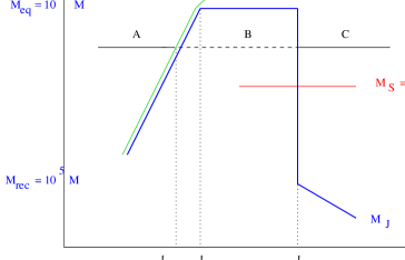
Figure 1: Typical evolution of a perturbed scale $M=M(\lambda)$ in adiabatic scenarios. During stage A ($t<t_{\rm ent}<t_{\rm eq}$) the mode grows as $\delta_{\rm b}\propto t$. Throughout stage B ($t_{\rm ent}<t<t_{\rm eq}$) the perturbation oscillates. Finally, in stage C ($t_{\rm rec}<t$) the mode becomes unstable again and grows as $\delta_{\rm b}\propto t^{2/3}$ Note that fluctuations with size smaller than $M_{\rm S}$ are wiped out by photon diffusion.

Schematically, the evolution of an adiabatic mode with mass scale $M(\lambda)$ is depicted in Figure 1. We distinguish between three evolutionary stages A, B and C, depending on the size of the perturbation and on the time of horizon crossing.

In adiabatic scenarios the smallest scales with any structure imprint upon them at the time of recombination are as large as a rich cluster of galaxies. Fluctuations on smaller scales have been completely obliterated by Silk damping. After decoupling perturbations grow steadily until their amplitude becomes of order unity or larger. At that point the linear theory breaks down and one needs to employ a different type of analysis. Qualitatively, what happens is that those huge perturbations undergo anisotropic collapse to form massive flattened objects known as “pancakes” or “caustics” (Zeldovich (1970) [16]). After pancake formation, non-linear gas dynamics inside the collapsed structure lead to shock generation and the subsequent cooling causes fragmentation into smaller structures. Thus, in the adiabatic scenario galaxies are born out of larger condensations in a “top-down” fashion. The expected large-scale structure pattern is one of large sheet-like filaments with enormous voids in between, a picture that seems to fit qualitatively very well with observations.

The main difficulty with the adiabatic scenario is that it predicts angular fluctuations in the CMB temperature in excess with observational limits. More specifically, in a $\Omega=1$ baryonic universe, one needs $\delta_{\rm b}\simeq 10^{-3}$ at recombination if structure were ever to form by today. In the adiabatic picture, however, matter inhomogeneities are accompanied by perturbations in the radiation field. This will inevitably lead to temperature fluctuations of order $\delta{\rm T}/{\rm T}\simeq\delta_{\gamma}\simeq 10^{-3}$ at decoupling, which is in direct disagreement with observations. To make things worse, primordial nucleosynthesis restricts the baryonic contribution to the total density of the universe down to $\Omega_{\rm b}\simeq 0.1$. Given that perturbations grow slower in open models than in flat ones, a greater temperature fluctuation at recombination is required if structure were to form by now.

4.6.2 Isothermal scenarios

In isothermal models structure formation proceeds very differently. Isothermal fluctuations remain frozen-in throughout the radiation era due to the radiation drag. After recombination modes larger than $(M_{\rm J}^{({\rm i})})_{\rm rec}\simeq 5\times 10^{5}(\Omega h^{2})^{-1/2}~{}{\rm M}_{\odot}$ are the first to collapse, while smaller scales are of no cosmological relevance. Thus, in the isothermal picture the first masses to condense out of the primordial plasma have the size of a globular cluster. These first structures start clustering together via gravitational instability to form successively larger agglomerations. In other words, galaxies and galaxy clusters form hierarchically in a “bottom up” fashion. Qualitatively, one expects to see a roughly self-similar clustering pattern without the dramatic structures of the adiabatic models.

Isothermal models do not have difficulties with the CMB anisotropies, since by definition the radiation field is uniformly distributed. In addition, the mass scale of the crucial first generation of structures is too small. The major problems with these scenarios is that the structure we see in the universe is not purely hierarchical. Galaxies have their own individual properties and galaxy clusters dot not just look like large galaxies. In the isothermal models this individuality of galaxies must be explained through some non-gravitational, probably dissipative, process. In addition, isothermal disturbances seem rather unnatural. Only very special physical processes can lead to primordial fluctuations in the matter component leaving the tightly coupled radiation field undisturbed. Particular inflationary models, where the scalar field responsible for generating the fluctuations is not the inflaton itself, may be able to produce this special type of perturbations.

5 Non-baryonic structure formation

The difficulties faced by the purely baryonic models opened the way for alternative structure formation scenarios, where the dominant matter is non-baryonic. Further motivation for considering models dominated by exotic matter species came from a combination of observational data and theoretical prejudice. Observations of the light element abundances, in particular, require $\Omega_{\rm b}h^{2}<0.015$ to comply with primordial nucleosynthesis calculations. On the other hand, dynamical considerations seem to imply that $\Omega\simeq 0.2$ and inflation argues for $\Omega\simeq 1$. If all these are true, our universe must be dominated by exotic non-baryonic species to the extent that the baryons are only a small fraction of the total matter.

5.1 Non-baryonic cosmic relics

An ongoing problem of the dark matter scenarios is that we still do not exactly know neither the nature nor the masses of the particles that make up the collisionless component of our universe. High energy physics theories, however, provide us with a whole “zoo” of candidates which are known as “cosmic relics” or “relic WIMPs”. Typically, we distinguish between “thermal” and “non-thermal” relics. The former are kept in thermal equilibrium with the rest of the universe until they decouple. A characteristic example of this relic type is the massless neutrino. Non-thermal relics on the other hand, such as axions, magnetic monopoles and cosmic strings, have been out of equilibrium throughout their lifetime. Thermal relics are further subdivided into “hot” relics, which are still relativistic when they decouple, and “cold” relics which go non-relativistic before decoupling. A typical hot thermal relic is a light neutrino with $m_{\nu}\simeq 10~{}{\rm eV}$. The best motivated cold relic is the lightest supersymmetric partner of the standard model particles, with a predicted $\Omega_{WIMP}\sim 1$. Note that thermal relics with masses around $1$ keV are usually referred to as “warm dark matter”. Right-handed neutrinos, axinos and gravitinos have all been suggested as potential warm relic candidates.

5.2 Evolution of the Jeans mass

If the dark component is made up of weakly interacting species, the particles do not feel each other’s presence via collisions. Each particle moves along a spacetime geodesic, while perturbations modify these geodesic orbits. One can study the response of the of the dark matter component by invoking an effective pressure and treating the collisionless species as an ideal fluid. The associated Jeans length is obtained similarly to the baryonic one. When dealing with a collisionless species, however, one needs to replace Eqs. (1), (2) with the Liouville equation (see Coles & Lucchin (1995) [8]). Then,

$$\lambda_{\rm J}=v_{\rm DM}\sqrt{\frac{\pi}{G\rho}}\,,$$ (77)

where now $v_{\rm DM}$ is the velocity dispersion of the dark matter component. The corresponding Jeans mass is

$$M_{\rm J}={\textstyle{4\over 3}}\pi\rho_{\rm DM}\left(\frac{\lambda_{\rm J}}{2}\right)^{3}\,,$$ (78)

where $\rho_{\rm DM}$ is the density of the non-baryonic matter.

5.2.1 Hot thermal relics

They decouple while they are still relativistic, that is $t_{\rm dec}<t_{\rm nr}$, where we assume that $t_{\rm nr}<t_{\rm eq}$. Throughout the relativistic regime $v_{\rm DM}\sim 1$, $\rho\simeq\rho_{\gamma}\propto a^{-4}$ and $\rho_{\rm DM}\propto a^{-4}$, implying that $\lambda_{\rm J}^{({\rm h})}\propto a^{2}$ and $M_{\rm J}^{({\rm h})}\propto a^{2}$. Once the species have become non-relativistic and until matter-radiation equality, $v_{\rm DM}\propto a^{-1}$, $\rho\simeq\rho_{\gamma}\propto a^{-4}$ and $\rho_{\rm DM}\propto a^{-3}$. Recall that the particles have already decoupled, which means that ${\rm T}_{\rm DM}\neq T_{\gamma}$. Consequently, $\lambda_{\rm J}^{({\rm h})}\propto a$ and $M_{\rm J}^{({\rm h})}={\rm constant}$. After equipartition $v_{\rm DM}\propto a^{-1}$ and $\rho\simeq\rho_{\rm DM}\propto a^{-3}$, which translates into $\lambda_{\rm J}^{({\rm h})}\propto a^{1/2}$ and $M_{\rm J}^{({\rm h})}\propto a^{-3/2}$. Overall, the Jeans mass of hot thermal relics evolves as

$$M_{\rm J}^{({\rm h})}\propto\left\{\begin{array}[]{l}a^{2}\hskip 56.9055ptz>z_{\rm nr}\,,\\ {\rm constant}\hskip 28.45274ptz_{\rm nr}>z>z_{\rm eq}\,,\\ a^{-3/2}\hskip 42.67912ptz_{\rm eq}>z\,.\end{array}\right.$$ (79)

Clearly, $M_{\rm J}^{({\rm h})}$ reaches its maximum at $z_{\rm nr}$. In fact, the highest possible value corresponds to particles with $z_{\rm nr}=z_{\rm eq}$ such as neutrinos with $m_{\nu}\simeq 10~{}{\rm eV}$. In this case $(M_{\rm J}^{({\nu})})_{\rm max}\simeq 3.5\times 10^{15}(\Omega_{\nu}h^{2})^{-2}~{}{\rm M}_{\odot}$ (see Coles & Lucchin (1995) [8]). For a typical hot thermal relic $(M_{\rm J}^{({\rm h})})_{\rm max}\sim 10^{12}-10^{14}~{}{\rm M}_{\odot}$.

5.2.2 Cold thermal relics

Cold thermal relics decouple when they are already non-relativistic (i.e. $t_{\rm nr}<t_{\rm dec}<t_{\rm eq}$). Thus, for $t<t_{\rm nr}$ we have $v_{\rm DM}\sim 1$, $\rho_{\rm DM}\propto a^{-4}$ and $\rho\simeq\rho_{\gamma}\propto a^{-4}$, implying that $\lambda_{\rm J}^{({\rm c})}\propto a^{2}$ and $M_{\rm J}^{({\rm c})}\propto a^{2}$. In the interval between $t_{\rm nr}$ and $t_{\rm dec}$ the key variables evolve as $v_{\rm DM}\propto a^{-1/2}$ (recall that ${\rm T}_{\rm DM}\simeq{\rm T}_{\gamma}$ until $t_{\rm dec}$), $\rho_{\rm DM}\propto a^{-3}$ and $\rho\simeq\rho_{\gamma}\propto a^{-4}$. As a result, $\lambda_{\rm J}^{({\rm c})}\propto a^{3/2}$ and $M_{\rm J}^{({\rm c})}\propto a^{3/2}$. After the particles have decoupled ${\rm T}_{\rm DM}\neq{\rm T}_{\gamma}$, which means that $v_{\rm DM}\propto a^{-1}$. At the same time $\rho_{\rm DM}\propto a^{-3}$ and $\rho\simeq\rho_{\gamma}\propto a^{-4}$, ensuring that $\lambda_{\rm J}^{({\rm c})}\propto a$ and $M_{\rm J}^{({\rm c})}={\rm constant}$. After equilibrium $v_{\rm DM}\propto a^{-1}$ and $\rho\propto\rho_{\rm DM}\propto a^{-3}$, implying that $\lambda_{\rm J}^{({\rm c})}\propto a^{1/2}$ and $M_{\rm J}^{({\rm c})}\propto a^{-3/2}$ In short, the Jeans mass of cold thermal relics evolves as

$$M_{\rm J}^{({\rm c})}\propto\left\{\begin{array}[]{l}a^{2}\hskip 56.9055ptz>z_{\rm nr}\,,\\ a^{3/2}\hskip 48.36967ptz_{\rm nr}>z>z_{\rm dec}\,,\\ {\rm constant}\hskip 28.45274ptz_{\rm dec}>z>z_{\rm eq}\,,\\ a^{-3/2}\hskip 42.67912ptz_{\rm eq}>z\,.\end{array}\right.$$ (80)

Accordingly, the maximum value for ${\rm M}_{\rm J}^{({\rm c})}$ corresponds to species with $t_{\rm dec}=t_{\rm eq}$. In other words, the sooner the particles cease being relativistic and decouple the smaller the associated maximum Jeans mass. Typically $(M_{\rm J}^{({\rm c})})_{\rm max}\ll 10^{12}~{}{\rm M}_{\odot}$.

5.3 Evolution of the Hubble mass

By definition

$$M_{H}={\textstyle{4\over 3}}\pi\rho_{\rm DM}\left(\frac{\lambda_{H}}{2}\right)^{3}\,,$$ (81)

where $\rho_{\rm DM}$ is the energy density of the collisionless species. For $t<t_{\rm nr}$ we have $\rho_{\rm DM}\propto a^{-4}$, $\lambda_{H}\propto t\propto a^{2}$. During the interval $t_{\rm nr}<t<t_{\rm eq}$ we have $\rho_{\rm DM}\propto a^{-3}$ and $\lambda_{H}\propto t\propto a^{2}$. Finally, when $t_{\rm eq}<t$, $\rho_{\rm DM}\propto a^{-3}$ and $\lambda_{H}\propto t\propto a^{3/2}$. Overall the Hubble mass of the dark matter component evolves as

$$M_{H}\propto\left\{\begin{array}[]{l}a^{2}\hskip 48.36967ptz>z_{\rm nr}\,,\\ a^{3}\hskip 48.36967ptz_{\rm nr}>z>z_{\rm eq}\,,\\ a^{3/2}\hskip 39.83385ptz_{\rm eq}>z\,.\end{array}\right.$$ (82)

Following definitions (77), (78) and (81), one can easily verify that the Jeans mass and the Hubble mass are effectively identical as long as the relic species are relativistic.

5.4 Dissipative effects

The ideal fluid approximation for collisionless species holds on sufficiently large scales only. On small scales, the free geodesic motion of the particles will wipe out any structure. This process is known as “Landau damping” or “free streaming”. A proper calculation of the damping scale associated to free streaming requires integrating the collisionless Boltzmann equation. Here, we will only obtain an estimate of the effect in the case of hot thermal relics. To begin with, consider the coordinate (comoving) distance travelled by a free streaming particle

$$x_{\rm FS}=\int_{0}^{t}\frac{v_{\rm DM}}{a}{\rm d}t\,,$$ (83)

where $\ell_{\rm FS}=ax_{\rm FS}$ is the corresponding physical (i.e. proper) distance. Clearly, perturbations in the dark matter component on scales smaller than $\ell_{\rm FS}$ will be wiped out by free streaming. Integrating the above we find, for $t<t_{\rm nr}$ when $v_{\rm DM}\sim 1$ and $a\propto t^{1/2}$

$$x_{\rm FS}=\frac{t_{\rm nr}^{1/2}}{a_{\rm nr}}\int_{0}^{t}\,t^{-1/2}{\rm d}t=\frac{2t_{\rm nr}^{1/2}}{a_{\rm nr}}t^{1/2}\,,$$ (84)

on using the relation $a=a_{\rm nr}(t/t_{\rm nr})^{1/2}$. The above suggests that $\ell_{\rm FS}=2t$ by the time the species have ceased being relativistic. During the interval $t_{\rm nr}<t<t_{\rm eq}$, when $v_{\rm DM}\propto a^{-1}$ (i.e. $v_{\rm DM}=a_{\rm nr}/a$) and $a\propto t^{1/2}$, the integration gives

$$x_{\rm FS}=\frac{2t_{\rm nr}}{a_{\rm nr}}+a_{\rm nr}\int_{t_{\rm nr}}^{t}\,a^{-2}{\rm d}t=\frac{2t_{\rm nr}}{a_{\rm nr}}\left[1+\ln\left(\frac{a}{a_{\rm nr}}\right)\right]\,,$$ (85)

where $2t_{\rm nr}/a_{\rm nr}$ is the coordinate free streaming distance at $t_{\rm nr}$. The associated physical free streaming scale is $\ell_{\rm FS}=ax_{\rm FS}=2t_{\rm nr}/a_{\rm nr}[1+\ln(a/a_{\rm nr})]a$. Finally, after equipartition $v_{\rm DM}\propto a^{-1}$ (i.e. $v_{\rm DM}=a_{\rm nr}/a$ still) and $a\propto t^{2/3}$. Thus, a further integration of Eq. (83) gives

$$x_{\rm FS} = \frac{2t_{\rm nr}}{a_{\rm nr}}\left[1+\ln\left(\frac{a_{\rm eq}}{a_{\rm nr}}\right)\right]+a_{\rm nr}\int_{t_{\rm nr}}^{t}\,a^{-2}{\rm d}t$$ (86)

$$= \frac{2t_{\rm nr}}{a_{\rm nr}}\left[1+\ln\left(\frac{a_{\rm eq}}{a_{\rm nr}}\right)\right]+\frac{3a_{\rm nr}t_{\rm eq}}{a_{\rm eq}^{2}}\left[1-\left(\frac{t_{\rm eq}}{t}\right)^{1/3}\right]$$

$$= \frac{2t_{\rm nr}}{a_{\rm nr}}\left[1+\ln\left(\frac{a_{\rm eq}}{a_{\rm nr}}\right)\right]+\frac{3t_{\rm eq}}{a_{\rm nr}}\left[1-\left(\frac{a_{\rm eq}}{a}\right)^{1/2}\right]\,,$$

on using the relation $t_{\rm eq}a_{\rm nr}^{2}=t_{\rm nr}a_{\rm eq}^{2}$. Thus, the total physical fee-streaming scale is

$$\ell_{\rm FS}=\left\{\frac{2t_{\rm nr}}{a_{\rm nr}}\left[1+\ln\left(\frac{a_{\rm eq}}{a_{\rm nr}}\right)\right]+\frac{3t_{\rm eq}}{a_{\rm nr}}\left[1-\left(\frac{a_{\rm eq}}{a}\right)^{1/2}\right]\right\}a\,.$$ (87)

At late times, when $a\gg a_{\rm eq}$, the above approaches its maximum value

$$\ell_{\rm FS}\rightarrow\left(\ell_{\rm FS}\right)_{\rm max}=\frac{t_{\rm nr}}{a_{\rm nr}}\left[5+2\ln\left(\frac{a_{\rm eq}}{a_{\rm nr}}\right)\right]\,,$$ (88)

where the scale factor has been normalized so that $a=1$ at present. To obtain numerical estimates we need to identify the epoch the species become non-relativistic. Assuming that the transition takes place when $T\sim m_{\rm DM}/3$ we find (see Padmanabhan (1993) [8])

$$\left(\ell_{\rm FS}\right)_{\rm max}\simeq 0.5\left(\frac{m_{\rm DM}}{1~{}{\rm keV}}\right)^{-4/3}\left(\Omega_{\rm DM}h^{2}\right)^{1/3}~{}{\rm Mpc}\,,$$ (89)

where $m_{\rm DM}$ is the mass of the collisionless particles in units of 1 keV. Accordingly, the minimum scale that survives collisionless dissipation depends crucially on the mass of the dark matter species. For neutrinos, with $m_{\rm\nu}\simeq 30$ eV we find $(\ell_{\rm FS})_{\rm max}\simeq 28$ Mpc and a corresponding mass scale $(M_{\rm FS})_{\rm max}\sim 10^{15}~{}{\rm M}_{\odot}$. Note that a more accurate treatment, using the Boltzmann equation, gives $\ell_{\rm FS}\simeq 40$ Mpc. For a much heavier candidate, say $m_{\rm DM}\simeq 1$ keV, we find $(\ell_{\rm FS})_{\rm max}\sim 0.5$ Mpc and $(M_{\rm FS})_{\rm max}\sim 10^{9}~{}{\rm M}_{\odot}$. In general, the lighter the dark matter species less power survives on small scales.

Cold thermal relics and non-thermal relics have very small dispersion velocities. As a result, the maximum values of the Jeans mass and of the free streaming mass are very law. In this case, perturbations on all scales of cosmological interest grow unimpeded by damping processes, although they suffer stagnation due to the Meszaros effect until matter-radiation equality. After recombination the potential wells of the collisionless species can boost the growth of perturbations in the baryonic component on scales of the order of $(M_{\rm J}^{({\rm i})})_{\rm rec}\sim 10^{5}~{}{\rm M}_{\odot}$.

5.5 Scenarios, successes and shortcomings

Historically, there have been two major non-baryonic structure formation scenarios. The “Hot Dark Matter” (HDM) models, where the dominant collisionless matter is in the form of hot thermal relics, and the “Cold Dark Matter” (CDM) models in which the baryonic component is either a cold thermal relic or a non-thermal species. It should be emphasized that, at present, pure HDM models are not considered viable and that the simplest CDM models are struggling to survive. Here, we will outline the key features of these two old adversaries and present some of the current alternatives.

5.5.1 Hot dark matter models

Typical HDM scenarios involve thermal relics with $z_{\rm nr}\simeq z_{\rm eq}$ and the best motivated candidate is a light neutrino species with $m_{\nu}\sim 10$ eV. The key feature of the perturbation spectrum is the cutoff at $\ell_{\rm FS}\simeq 40$ Mpc due to the neutrino free streaming. Because of this, the first structures to form have sizes of approximately $10^{15}\,{\rm M}_{\odot}$ which corresponds to a supercluster of galaxies (see Figure 2). Moreover, because the scale is very large collapse must have occurred at relatively recent times (i.e. at $z<3$). Thus, in a universe dominated by hot thermal relics, structure formation proceeds in a top-down fashion similar to the adiabatic baryonic models. Perturbations on scales as large as $10^{15}\,{\rm M}_{\odot}$ go no linear in a highly non-spherical way. As a result, they collapse to one dimensional objects resembling the pancake-like formations of the baryonic models (Zeldovich (1970) [16]). Once the pancake forms and goes non-linear in one of its dimensions, the baryons within start colliding with each other and dissipate their energy. Thereby, the baryonic component fragments and condenses into smaller galaxy-sized objects. The neutrinos, however, do not collide neither with each other nor with the baryons. They are therefore unable to dissipate their energy and collapse into more tightly bound objects. They remain less condensed forming what one might call a “neutrino halo” around the baryons.

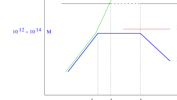
Figure 2: Typical evolution of a perturbed scale $M=M(\lambda)$ in HDM scenarios. During stage A ($t<t_{\rm ent}<t_{\rm eq}$) the mode grows as $\delta_{\rm DM}\propto t$. Throughout stage B ($t_{\rm ent}<t<t_{\rm eq}$) the perturbation is frozen in due to the Meszaros effect. Finally, in stage C ($t_{\rm rec}<t$) the mode becomes unstable again and grows as $\delta_{\rm b}\propto t^{2/3}$ Note that fluctuations with size smaller than $M_{\rm FS}$ are wiped out by neutrino free streaming.

Several groups have numerically simulated structure formation in a neutrino dominated universe (e.g. Centrella & Mellott (1982); White et al (1983) [18]). In all simulations one notices a cell-like structure, which reflects the damping scale due to neutrino free streaming. The structure of these simulations on scales larger than $10$ Mpc is qualitatively similar to the voids and filaments seen in some of the redshift surveys. However, the models have problems reproducing the small scale clustering properties of galaxies. In particular, the HDM simulations can agree with the observed galaxy-galaxy correlation function only if the epoch of pancaking takes place at $z\simeq 1$ or less. This seems too late to account for the existence of galaxies with redshift $z>1$ and of quasars with $z\simeq 5$. A possible way out is if the density field of the universe is traced by galaxy clusters rather than by galaxies themselves. In this case the mismatch between the predicted and the observed amount of small-scale structure is alleviated. An additional problem of the HDM scenarios is that the baryons are shock heated as they fall into the pancakes. This might have raised the temperature to levels that could have prevented the baryonic matter from condensing or led to excessive x-ray production.

5.5.2 Cold dark matter models

Cold dark matter (CDM) candidates are cold thermal relics and non-thermal relics with $z_{\rm nr}\ll z_{\rm eq}$. For such particles the maximum damping scale is too small ($\ll 1$ Mpc) to be of any cosmological relevance. In the CDM models the important feature is the weak growth experienced by perturbations between horizon crossing and equipartition. It means that the density contrast increases as we move to smaller scales, or that the perturbation spectrum has more small-scale power. Note that the shape of the HDM spectrum in not cosmologically important, as the minimum scales to survive free streaming are way too large. Thus in standard CDM scenarios the first objects to break away from the background expansion have sub-galactic sizes ($<10^{6}~{}{\rm M}_{\odot}$). These structures virialize through violent relaxation (Lynden-Bell (1967); Shu (1978) [17]) into gravitationally bound configurations that resemble galactic halos. At the same time the baryons can dissipate their energy and condense further into the cores of these objects. As larger and larger scales go non-linear, bigger structures form through tidal interactions and mergers. Hence, according to the CDM scenario structure forms in a bottom-up fashion analogous to that of the isothermal baryonic models. Note that the ability of baryons to dissipate allows objects of astrophysical size to condense out as individual and discrete entities. The predicted properties of the different kinds of galaxies that form this way appear in good agreement with observations (Blumenthal et al (1984) [19]).

The simplest CDM scenario, now known as the “Standard CDM” (SCDM) model, has critical density and contains only cold collisionless species (Peebles (1982); Blumenthal et al (1984); Davis et al (1985, 1992) [19]). Major problems with these scenarios are their failure of the simulations to reproduce the observed galaxy-galaxy correlation function and the overproduction of clusters when the modes are normalized with the COBE results. One can attempt to save the SCDM model by removing the excess small-scale power from the perturbation spectrum, an approach known as tilting of the spectrum, (Vittorio et al (1988); Bond (1992); Liddle et al (1992) [20]). This strategy, however, usually has disastrous effects on the acoustic peaks of the CMB. At the moment, the only way out for the SCDM model is a baryon density substantially higher than the one predicted by standard nucleosynthesis (White et al (1995b, 1996) [21]).

5.5.3 Alternative options

In an effort to salvage critical density, researchers have abandoned the CDM hypothesis in favor of a mixture of cold and hot dark matter particles (Bonommetto & Valdarnini (1984); Fang et al (1984); Shafi & Stecker (1984); Holtzman (1989); Schaefer et al (1989) [22]). Hybrid “Cold-Hot Dark Matter” (CHDM) scenarios take advantage of the free streaming properties of their hot collisionless component to reduce the small-scale power in the perturbation spectrum. The original version had $\Omega_{\rm CDM}=0.7$ and $\Omega_{\rm HDM}=0.3$ (Davis et al (1992); Schaefer & Shafi (1992, 1994); Taylor & Rowan-Robinson (1992); Klypin et al (1994) [23]), but the free streaming effect was too strong. Currently, the preferred values for the hot dark matter contribution lie near $\Omega_{\rm HDM}=0.2$ (Klypin et at (1995); Pogosyan & Starobinski (1995); Liddle et al (1996) [24]). Note that CHDM models require a rather uncomfortable fine-tuning to produce two particle species with similar cosmological densities but very different masses.

If one wants to retain the CDM hypothesis, namely to assume cold collisionless species only, the simple strategy is to reduce the matter density. This shifts matter-radiation equality to a later epoch, lengthening the period in which the small-scale modes have their growth suppressed. In view of the very different normalization of low-density universes with the COBE data, models with $\Omega\simeq 0.3$ ought to be easily distinguishable from those with critical density. This is not the case, however, since most other observations also require analogous renormalizations.

The natural way of keeping the low-density models compatible with standard inflation is to introduce a cosmological constant, thus obtaining the $\Lambda$CDM scenarios (Peebles (1984); Turner et al (1984); Efstathiou et at (1990); Ostriker and Steinhardt (1995) [25]). Note that, at present, a non-zero cosmological constant is favoured by the type-Ia suprenovae measurements (Perlmutter et al, (1998); Schmidt et al (1998) [26]). The presence of a non-zero $\Lambda$ means that one can capitalize on the freedom to vary the rest of the parameters. At the moment it appears that $\Omega\simeq 0.3$ is the allowed lower limit on the density, with the optimum value near $\Omega=0.3$. Note that one can achieve extra freedom by assuming that the cosmological constant is actually a decaying function of time, which is usually referred to as “quintessence” (Coble et al (1997); Turner & White (1997); Caldwell et al (1998) [27])

An alternative way of shifting the time of equipartition is by adding extra massless species in the model (Bardeen et al (1987); Bond and Efstathiou (1991) [28]). Recall that the present density in relativistic particles is not known since the neutrino background remains undetectable. Note, however, that the presence of relativistic species is strongly constrained by nucleosynthesis, which means that the extra relativistic energy must be generated later on (Dodelson et al (1994); McNally & Peacock (1995); White et al (1995a) [29]).

In all of the aforementioned models the perturbations are of the adiabatic type. Scenarios based on pure isocurvature fluctuations do not seem viable. However, an admixture of adiabatic and isocurvature modes has not been excluded. In fact, the COBE data do not seem to discriminate against an isocurvature component (Stompor et al (1996) [30]).

Topological defects, such as cosmic strings, monopoles domain walls and textures, provide a very different alternative to structure formation (Vilenkin & Shellard (1994); Hindmarsh & Kibble (1995) [3]). They have much more predictive power than inflation, but they are also more technically demanding. Moreover, current observations appear unfavorable to them (Allen et al (1997); Pen et al (1997) [31]).

6 Discussion

The question of how the observed large-scale structure of the universe developed and how galaxies were formed has been one of the outstanding problems in modern cosmology. Looking back into the past hundred years one sees three decisive moments in the pursuit of the answer. The first milestone was the formulation of general relativity which provided researchers with the theoretical tool to probe the large-scale properties of the universe. Hubble’s observations manifesting the expansion of the universe was the second decisive moment, as it forced cosmologists to break away from the then prevailing concepts of a static and never-changing cosmos. Finally, the discovery of the Cosmic Microwave Background radiation by Penzias and Wilson established the Hot Big Bang theory, an idea advocated several years earlier primarily by Gamov. At last, cosmologists had a definite model within which they could tackle the structure formation question. Pending future observations, one could argue that the inflationary paradigm is one additional milestone in our effort to understand the workings of our universe. The recent supernovae measurements, which suggest an accelerated universal expansion, could prove another very decisive moment. Time will show whether they actually are.

Despite the problems and the uncertainties, cosmologists now believe that all the structure that we observe around us today originated from minute perturbations in a cosmic fluid that was smooth to the accuracy of one part in ten thousand at the time of recombination. Such tiny irregularities could have been triggered by quantum fluctuations that were stretched out during the inflationary expansion or by topological defects such as cosmic strings for example. Given the current observational status, inflation appears to be the strongest candidate. In these notes we have set aside the question of the origin of the primeval fluctuations. Our discussion focussed on the linear evolution of these minute irregularities once the universe entered the post-inflationary Hot Big Bang era, and on the physical processes that could have affected them. When studying density perturbations, one sooner or later encounters the reality that baryon inhomogeneities cannot actually grow before recombination. This fact, together with the extreme smoothness of the CMB temperature, implies that baryonic fluctuations simply do not have enough time to produce the observed structure. When one adds to that the nucleosythesis constraints and the strong theoretical and observational bias for spatial flatness, the once popular baryon-dominated picture of the universe seems unsustainable. So, if the baryons are not the dominant form of matter in our universe, then what is? The answer to that might lie in high energy physics theories. Theoretical physics provides a whole zoo of supersymmetric, dark matter species that could bring $\Omega$ close to unity and also “assist” structure formation. The attractive feature of collisionless matter is that perturbations in its density start growing earlier than those in the baryonic component. Thus, as soon as the baryons decouple from radiation, they undergo a period of fast growth as they fall into the potential wells of the collisionless species. This can improve the final picture but unfortunately does not solve all the problems. The key obstacle being that a single collisionless species does not seem capable of fitting all the data. At best, one needs the presence of one cold and one hot dark matter species in a combination that will make the most of their advantages while minimizing their shortcomings. The recent supernovae results, suggesting that our universe might be dominated by some sort of dark energy have added extra flavor to the whole situation. The presence of a cosmological constant, or quintessence, means that researchers have extra freedom when dealing with crucial cosmological parameters, such as the age of the universe for example. On the other hand, however, the idea that the majority of the matter in our universe is in the form of some unknown exotic species brings back some rather embarrassing memories from our relatively recent past. A lot could be decided within the next few years as we expect an influx of high quality data. The “Boomerang” and “Maxima” observations have added valuable information which seems to favor the inflation based models. The near future “Probe” and “Planck” satellite missions also promise high precision data. For some researchers structure formation is a story that is fast reaching its conclusion. The future will show if they are right or just too hasty.

References

- [1] J. Jeans: Phil Trans. 199A, 49 (1902); J. Jeans: Astronomy and Cosmology, Cambridge University Press (1928).
- [2] A.H. Guth: Phys. Rev. D 23, 347 (1981); A.D. Linde: Pys. lett. B 108, 389 (1982); A. Albrecht and P.J. Steinhardt: Phys. Rev. Lett. 48, 1220 (1982).
- [3] T.W.B. Kibble: J. Phys. A9, 1387 (1976); A. Vilenkin and E.P.S. Shellard: Cosmic Strings and Topological Defects, Cambridge University Press (1994); M.B. Hindmarsh and T.W.B. Kibble: Rep. Prog. Phys. 58, 477 (1995).
- [4] R. Harrison: Phys. Rev. D 1, 2726 (1970); Y.B. Zeldovich: Astron. Atrophys. 5, 84 (1970).
- [5] W.B. Bonnor: Mon. Not. R. Astron. Soc. 117, 104 (1957).
- [6] E.M. Lifshitz: J. Phys. (Moscow) 10, 116 (1946); E.M. Lifshitz and I.M. Khalatnikov: Adv. Phys. 12, 185 (1963).
- [7] S. Weinberg: Gravitation and Cosmology, Wiley (1972); L.D. Landau and E.M. Lifshitz: The Classical Theory of Fields, Pergamon Press (1975); P.J.E. Peebles: The large Scale Structure of the Universe, Princeton University Press (1980); W.H. Press and E.T. Vishniac: Astrophys. J. 239, 1 (1980).
- [8] E.W. Kolb and M.S. Turner: The Early Universe, Addison-Wesley (1990); T. Padmanabhan: Structure Formation in the Universe, Cambridge University Press (1993); P.J.E. Pebles Principles of Physical Cosmology, Princeton University Press (1993); P. Coles and F. Lucchin: Cosmology: The Origin and Evolution of Cosmic Structure, Wiley (1995); J.A. Peacock: Cosmological Physics, Cambridge University Press (1999); A.R. Liddle and D.H. Lyth: Cosmological Inflation and Large-Scale Structure, Cambridge University Press (2000).
- [9] P. Meszaros: Astron. Astrophys. 37, 225 (1974).
- [10] R. Sachs: in Relativity, Groups and Topology, eds. De Witt and DeWitt, Gordon and Breach (1964); J. Stewart: Class. Quantum Grav. 7, 1169 (1990); M. Bruni, P.K.S. Dunsby and G.F.R. Ellis: Astrophys. J. 395, 34 (1992).
- [11] J.M Bardeen: Phys. Rev. D 22, 1882 (1980); J.M. Bardeen, P.J. Steinhardt and M.S. Turner: Phys. Rev. D 28, 679 (1983); U.H. Gerlach and U.K. Sengupta: Phys. Rev. D 18, 1789 (1978); H. Kodama and M. Sasaki: Prog. Theo. Phys. suppl. 78, 1 (1984).
- [12] G.F.R Ellis and M. Bruni: Phys. Rev. D 40, 1804 (1989); S.W. Hwawking: Ap. J. 145, 544 (1966); J. Stewart and M. Walker: Proc. R. Soc. London A341, 49 (1974); D.W. Olson: Phys. Rev. D 14, 327 (1976).
- [13] G.F.R. Ellis and H. van Elst: in Theoretical and Observational cosmology, edited by M. Lachièze-Rey (Kluwer, Dordrecht, 1999)
- [14] Y.B. Zeldovich: Soviet Phys. Usp. 9, 602 (1967)
- [15] J. Silk: Nature 215, 1155 (1967); J. Silk: Ap. J. 151, 459 (1968); G. Efstathiou and J. Silk,: Fond. Cosmic Phys. 9, 1 (1983).
- [16] Y.B. Zeldovich: Astrofisika 6, 319 (1970).
- [17] D. Lynden-Bell: Mon. Not. R. Astron. Soc. 136, 101 (1967); F.H. Shu: Astrophys. J. 225, 83 (1978).
- [18] J. Centrella and A. Mellott: Nature 305, 196 (1982); S.D.M. White, C. Frenk and M. Davis: Ap. J. 274, L1 (1983); ibid 287, 1 (1983).
- [19] P.J.E. Peebles: Astrophys. J. 263, L1 (1982); G.R. Blumenthal, S.M. Faber, J.R. Primack and M.J. Rees: Nature 311, 517 (1984); M. Davis, G. Efstathiou, C. Frenk and S.D.M. White: Astrophys. J. 292, 271 (1985); M. Davis, G. Efstathiou, C. Frenk and S.D.M. White: Nature 356, 489 (1992).
- [20] N. Vittorio, S. Matarrese and F. Lucchin: Atrophys. J. 328, 69 (1988); J.R. Bond: in Highlights in Astronomy, Vol. 9, Proceedings of the IAU Joint Discussion, ed. J. Berjeron, Kluwer, Dordrecht (1992); A.R. Liddle, D.H. Lyth and W. Sutherland: Phys. Lett. B 279, 244 (1992).
- [21] M. White, D. Scott, J. Silk and M. Davis: Mon. Not. R. Astron. Soc. 276, L69 (1995b); M. White, P.T.P. Viana, A.R. Liddle and D. Scott: Mon. Not. R. Astron. Soc. 283, 107 (1996).
- [22] S.A. Bonommetto and R. Valdarnini: Phys. Lett. A 103 369 (1984); L.Z. Fang, S.X. Li and S.P. Xiang: Astron. Astrophys. 140, 77 (1984); Q. Shafi and F.W. Stecker: Phys. Rev. Lett. 53, 1292 (1984); J. Holtzman: Astrophys. J. Supp. 71, 1 (1989); R.K. Schaefer, Q. Shafi and F.W. Stecker: strophys. J. 347, 575 (1989).
- [23] M. Davis, F. Summers and D. Schlegel: Nature 359, 393 (1992); R.K. Schaefer and Q. Shafi: Nature 359, 199 (1992); R.K. Schaefer and Q. Shafi: Phys. Rev. D 49, 4990 (1994); A.N. Taylor and M. Rowan-Robinson: Nature 359, 396 (1992); A. Klypin, J. Holtzman, J.R. Primack and E. Regös: Astrophys. J. 416, 1 (1994).
- [24] A. Klypin, S. Borgani, J. Holtzman and J.R. Primack: Astrophys. J. 444, 1 (1995); D.Y. Pogosyan and A.A. Starobinski: Astrophys. J. 447, 465 (195); A.R. Liddle, D.H. Lyth, R.K. Shaefer, Q. Shafi and P.T.P. Viana: Mon. Not. R. Astron. Soc. 281, 531 (1996).
- [25] P.J.E. Peebles: Astrophys. J. 284, 439 (1984); M.S. Turner, G. Steigman and L.M. Krauss: Phys. Rev. Lett. 52, 2090 (1984); J.P. Ostriker and P.J. Steinhardt: Nature 377, 600 (1995).
- [26] S. Perlmutter et al: Nature 391, 51 (1998); B.P. Schmidt et al: Astrophys. J. 507, 46 (1998).
- [27] K. Coble, S. Dodelson and J.A. Frieman: Phys. Rev. D 55, 1851 (1997); M.S. Turner and M. White: Phys. Rev. D 56, R4439 (1997); R.R. Caldwell, R. Dave and P.J. Steinhardt: Phys. Rev. Lett. 80, 1586 (1998).
- [28] J.M. Bardeen, J.R. Bond and G. Efstathiou: Astrophys. J. 321, 28 (1987); J.R. Bond and G. Efstathiou: Phys. lett. B 265, 245 (1991);
- [29] S. Dodelson, G. Gyuk and M.S. Turner: Phys. Rev. Lett. 72, 3754 (1994); S.J. Mcnally and J.A. Peacock: Mon. Not. R. Astron. Soc. 277, 143 (1995); M. White, G. Gelmini and J. Silk: Phys. Rev. D 51, 2669 (1995a).
- [30] R. Stompor, K.M. Górski and A.J. Banday: Astrophys. J. 463, 8 (1996).
- [31] B. Allen, R.R. Caldwell, S. Dodelson, L. Knox, E.P.S. Shellard and A. Stebbins: Phys. Rev. lett. 79, 2624 (1997); U.L. Penn, U. Seljak and N. Turok: Phys. Rev. Lett. 79, 1611 (1997).