An attempt to model globular cluster red giant abundance anomalies with a simulated hydrogen shell instability

Abstract

It has been suggested that the anomalous Na, Mg and Al observed in Globular Cluster Red Giant stars could be the result of a thermally unstable hydrogen shell. Currently accepted reaction rates indicate that temperatures of approximately 70-75 million K are required to produce the observed enhancements in Na and Al along with depletions in Mg.

The work presented here attempts to model the H shell instability by a simple mechanism of altering the energy production in the region of the H shell. We show that even extreme cases only give rise to small intermittent temperature increases that have minimal affect on the surface abundances. Full evolutionary modelling incorporating this technique simply accelerates the evolution of the RGB phase producing the same surface abundances as other models but at an earlier time. We conclude that, unless hydrogen shell instabilities manifest themselves quite differently, they are unlikely to lead to the required temperatures and alternative explanations of the abundance anomalies are more promising.

1 Introduction

As long ago as 1947, Popper [1947] had noted that the globular cluster red giant L199 in M13 was CN-strong. Further work by Harding [1962], Osborn [1971] and Hesser, Hartwick and McClure [1976] confirmed that this anomaly is common. So for over fifty years it has been known that the surface abundances of elements such as C and N can vary from one red giant star to another within an individual globular cluster. It has become clear in the intervening years, however, that these anomalies are not restricted to C and N: heavier elements such as O, Na, Mg and Al also show star to star variations. Most other elements studied show little variation, and the degree of variation of C, N, O etc. differs from cluster to cluster and is much less apparent in field stars [1992].

Observations by many groups, including Kraft et al. [1997], Smith and Kraft [1996], Langer [1992], Shetrone [1996a] [1996b] [1997], have identified this abundance anomaly problem and the most commonly suggested explanation for such high Na and Al are the deep mixing [1979] and primordial enhancement [1981] hypotheses. The deep mixing hypothesis suggests that the rotation of the star can give rise to meridional circulation currents that in turn create a mixing zone in the radiative region separating the top of the hydrogen burning shell (HBS) and the base of the convective envelope (BCE). This would allow elements processed in the HBS to be mixed to the surface as the star proceeds up the RGB. The primordial enhancement hypothesis suggests that the stars are born with these anomalies already present. The stars are formed from material ejected by intermediate mass ($\simeq 3-10M_{\odot}$) AGB stars from an earlier epoch. Without going into the full mechanisms of each process, either could in principle explain the observed anomalies, but modelling and observations have indicated that probably both processes occur to some extent.

Langer, Hoffman and Zaidins [1997] suggested that the Na and Al abundance anomaly problem may be solved if the H shell reached higher temperatures for at least part of its lifetime whilst on the RGB. The idea stems from work by Von Rudloff and Vandenburg [1988] and even earlier work by Bolton and Eggleton [1973]. Von Rudloff and Vandenburg [1988] found that the H shell of a non-rotating small mass red giant model was stable but only marginally. A rotating model could be unstable. The link with rotation is particularly encouraging because this mechanism could explain both the deep mixing and the thermally unstable shell. The work performed by Langer et al [1997] shows that a thermally unstable H shell would allow for the greater production of ²⁷Al at the expense of ²⁴Mg and that there would also be extra ²³Na available for mixing to the surface.

The conclusion was that if the H shell reached temperatures of approximately 70-75 million K then the material mixed to the surface would produce a composition in close agreement with observation. In fact temperatures of this order and no lower would be required to match the Na observations because at the lower temperatures too much ²³Na would be produced. Also it is only at these temperatures that significant ²⁷Al is produced and ²⁴Mg is only destroyed at temperatures above 70 million K. Therefore, to have any surface depletions in ²⁴Mg the temperature of the H shell has to reach at least 70 million K unless primordial changes are invoked or the accepted reaction rates are altered. The preferred temperature range was 72-73 million K (see section 2 of Langer et. al [1997]). This is the temperature at which they believed all the observed surface abundance anomalies could be matched.

As the structure of a model is heavily dependent upon the temperature profile any change to the temperature must be included in the evolution modelling. The following sections discuss models where temperatures in the H shell are artificially increased by decreasing the energy generation rate. The next section looks at oscillating temperature rises in the HBS; i.e. a pulsating model where each pulse immediately follows the previous pulse. In the following section pulses in the temperature of the HBS are created with a time gap between each pulse.

2 Computer Codes

The calculations reported here make use of two separate computer codes: the Monash/Mt Stromlo stellar evolution code, with which we model the evolution of stars from contraction to the main sequence up to the RGB tip, and a post-processing nucleosynthesis code [1990], with which we model the abundances within the star for the same epoch. The nucleosynthesis code uses the independent variables from the evolution code for its structural basis, with typically every sixth evolution model being used. The full details of how these two codes work and interface can be found in Messenger [2000].

The postulated deep mixing has been included in the nucleosynthesis code, and is described by three parameters - the depth, the speed and the time of onset of the deep mixing. We measure the depth in the same way as Wasserburg, Boothroyd and Sackmann [1997], by mixing down to a temperature $\triangle\log T$ above the base of the HBS, which is defined as the first point (moving outward from the center) to have a non-zero hydrogen abundance. This mixing commences once the HBS burns through the discontinuity left from the first dredge-up episode earlier in the evolution. Prior to this time it is assumed that this molecular weight discontinuity will inhibit mixing: once it is removed, the mixing is assumed to begin. Finally, we found (in agreement with previous researchers) that provided the speed of mixing was above a small critical value, it made almost no difference to the abundance patterns. We used a mixing speed of $10^{-4}M_{\odot}$/year in all calculations reported here.

In the work of Messenger [2000] it was found that varying the mixing depth as the star ascends the RGB gives better agreement with observations of Na. Therefore this type of modelling is adopted in this paper, and the mixing depth was changed linearly from an initial setting $\triangle\log T=0.18$ to $\triangle\log T=0.03$ as the star ascended the RGB.

3 Increased H shell Temperatures

3.1 Algorithm

To increase the temperature of the H shell it is not simply a matter of arbitrarily adding temperature to the mesh points within the shell. The temperature is one of the dependent structure variables and affects other variables such as the density and pressure through the equation of state. To self-consistently increase the temperature we chose to change the energy generation of the shell by increasing or decreasing the energy production rate for each point if it is within the boundaries of the H shell.

An increase of the energy generation rate causes the star to expand and the temperature to decrease. A reduction in the energy generation rate causes the opposite; the star contracts and the temperature increases. Therefore it was necessary to decrease the energy rate from H burning in order to artificially create a temperature increase.

A factor for the energy generation rate reduction, designated as $g$, was introduced. This reduction is only initiated after the H shell passes through the $\mu$-discontinuity remaining from the first dredge-up episode. The desired nuclear energy generation rate at a point in the H shell (when this feature is switched on) is

$$\indent\indent\indent\indent\epsilon_{used}=\epsilon_{rate}(1-g)$$ (1)

However, it is not simply a matter of reducing the energy generation rate over the full shell. This would create a large jump in energy generaqtion from the point just below the shell and also from the point at the top of the shell. It is necessary to linearly interpolate from 0 to the value of $g$ over a number of mesh points at the bottom of the shell and from $g$ to 0 at the top of the shell.

Let $h_{m}$ be the mesh-based linear interpolation factor. This varies from zero at the bottom of the HBS to a maximum of $g$ over $n$ mesh-points, remains at this maximum over $2n$ mesh points, and then decreases linearly over the next $n$ mesh points to a value of zero again. This is shown in Figure 1.

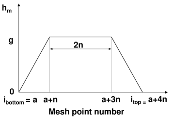
Figure 1: Basic energy generation rate reduction algorithm. The mesh-based energy generation reduction factor $h_{m}$ is linearly increased from zero to $g$ over $n$ mesh points, held at $g$ for $2n$ mesh points and then linearly decreased to zero over a further $n$ mesh points.

Once $h_{m}$ has been determined the energy generation rate remaining at any point within the H shell (as long as the H shell instability feature is switched on) is

$$\indent\indent\indent\indent\epsilon_{used}=\epsilon_{rate}(1-h_{m})$$ (2)

This alone caused a temporal discontinuity in the models and subsequently created convergence problems. Remember that this arbitrary temperature rise is non-physical. To avoid these convergence problems it was necessary to smoothly introduce the reduced energy generation rate in time as well as in mass (i.e. to gradually turn on the energy reduction). We introduce the reduction rate gradually over time with a parameter $h_{t}$ which is linearly increased from 0 to 1 over 20 timesteps. Thus the energy generation rate within the H shell is

$$\indent\indent\indent\indent\epsilon_{used}=\epsilon_{rate}(1-h_{m}h_{t})$$ (3)

Note that parametrisations in terms of mesh point (rather than mass) and model number (rather than time) are purely numerical conveniences. In reality, of course, these variations should be dependent on mass and time, but without any identified mechanism for the instability, and in view of the exploratory nature of the calculations reported here, we believe this simplification is justified and in no way affects our conclusions, which depend only on the shell temperature.

3.2 Results

All calculations reported here are carried out for a star of $0.8M_{\odot}$ with a metallicity of $Z=0.0005$. Parameters relevant to the deep mixing were given above.

The temperature in the H shell is determined by the requirement that the energy production rate be high enough to support the outer layers of the star. With a decreased rate of energy generation at a given temperature, the star’s response is to increase the temperature in the H shell. As the star evolves up the RGB, the H shell progresses outwards and thins. The higher temperatures mimic this process and the final result is an acceleration of the star’s evolution. This is shown in figure 2, where plots of luminosity against time for differing values of $g$ are shown. The greater the energy rate reduction, the quicker the star evolves to the RGB tip.

Figure 2: Model for a constant energy generation rate reduction. As can be seen the greater the reduction of the nuclear burning energy rate, the more rapid the evolution of the model. For $g=0.5$ the time spent on the RGB (since first dredge-up) is approximately 7.3% less than a star where $g=0$. Similarly for $g=0.8$ the time spent is approximately 12% less and for $g=1.0$ the time spent is approximately 16% less.

This result will not assist in the abundance anomaly problem because any enhancements/depletions will still occur to about the same degree as before but just at an earlier epoch. The higher temperatures within the H shell mimic normal evolution but reach it at an earlier stage. All this manages to do is force the model to the He flash more quickly. No extra Na, Mg or Al would be produced in this situation. in fact, with a reduced timescale for the burning, the effect may be the opposite of what is required, but in any event it will be quantitatively negligible.

4 Intermittent Temperature Rises

Langer et. al. [1997] suggested that the H shell is a thermally unstable region and that under certain conditions the shell may give rise to higher temperatures than standard physics suggests. The modelling performed in the previous section is not that of a thermally unstable region, but just a consistently higher temperature. To model a thermal instability the energy generation rate modification must not be steady but should be periodic or at least variable. A small modification to the algorithm of section 3 was therefore made to simulate a thermally unstable H shell.

The simplest way to do this is to continue to use the time based rate reduction algorithm but just make it periodic. Here the energy generation rate reduction was introduced over five timesteps, held at the peak for 20 timesteps and then decreased over another five timesteps. This was then repeated until the RGB tip was reached. For an initial test and to determine how pulsation may affect convergence there was no gap between each pulse. Apart from the increase and decrease of each pulse the affect would be identical to the continuous algorithm described in the previous section. We would therefore expect little change from the model for the previous algorithm and that is exactly the case. Figure 3 which has $g=0.8$ shows that the result of the above algorithm is to accelerate the evolution just as it did for the case of a continuous H shell temperature rise. The problem with the above approach is that the decrease in the energy generation rate causes the shell to contract and temperatures to rise. This shifts the star to a different evolutionary track. Once the energy generation rate returns to normal values the shell begins to expand again but there is not enough time for the star to settle back to its original (or close to original) evolutionary track before the next pulse begins. The end result is that the star shifts from its original evolutionary track and diverges from it henceforth.

If we do not want to significantly alter the evolution of the star, then it is necessary to introduce a time delay between pulses which is long enough for the star to resettle to its original track.

Figure 3: A periodic energy generation rate reduction model and a standard model with normal energy production.

We use a simple method, but it is efficient and can test the concept of a H shell instability without the introduction of large amounts of complex code which is hard to justify since there is no confirmed mechanism for the instability. The purpose of our algorithm is to test the principle of a periodic H shell instability, not the details. We use a technique similar in principle to that shown in figure 1 but we introduce periodicity and time delays between pulses. We firstly select the desired number of pulses between FDU and the tip of the giant branch. We thus determine the inter-pulse duration and distribute the pulses evenly over the giant branch life-time. After some experimentation we decided to use 20 pulses because this allows the star to settle back to its standard evolutionary track and it should illustrate any differences likely to occur due to the pulses. We then take as a characteristic time-scale the time-step used to construct the current model, which we denote as $dt$. Next, the duration of a pulse is taken as $30dt$, comprising $5dt$ over which we linearly increase $h_{t}$ from zero to unity, then $20dt$ using $h_{t}=1$, and a further $5dt$ when $h_{t}$ is linearly decreased back to zero. Of course, the time-steps used by the code vary, and are not all equal to $dt$ during the pulse, but $dt$ gives a convenient timescale for the test. Also, because the time-steps vary with evolution along the giant branch, the $dt$ used for each of the 20 pulses will be slightly different, but this is not important for our exploratory calculations.

The result of the introduction of this algorithm is shown in figure 4. The points that should be noted are the decrease in the luminosity shown during a pulse accompanied by a temperature increase and the fact that the curve and hence the model settles back to its original track. It is only at the latter stages of the RGB evolution that the curves begin to diverge.

The conclusion drawn from this model is that the H shell temperature can be increased intermittently without significantly affecting the evolution of the star. But how will it affect the nucleosynthesis of the model? Is the temperature increase high enough and long enough to produce significant amounts of ²⁷Al and reduce ²⁴Mg as originally hoped? It is necessary to look at the temperatures within the H shell to see whether temperatures of approximately 70 million K are reached, the temperature at which ²⁷Al enhancements are reasonable and ²⁴Mg depletions begin. Figure 5 shows the temperature at the base of the H shell as the star ascends the RGB for an energy generation rate reduction of 50% ($g=0.5$). The peak temperature reached by any of the pulses is only increased very slightly, well short of the required temperatures for ²⁴Mg destruction. Even a 100% reduction of the nuclear burning energy generation rate ($g=1.0$) during a pulse, as shown in figure 6, cannot produce high enough temperatures within the shell for the processes discussed here. For a test case, some of the gravitational and neutrino energy generation rates were also reduced ($g=1.5$). This created a minor increase in the temperature (see figure 7), but the peak temperature still fell short of the required temperatures.

Figure 4: Periodic energy generation rate reduction model and a standard model with no energy generation rate modifications. Here the evolution is not accelerated as much because there is enough time between pulses to allow the model to resettle on to its original evolutionary track. The model does deviate as it approaches the RGB tip but this could be avoided by selecting a smaller number of pulses.

Figure 5: The temperature at the base of the hydrogen shell for a periodic energy generation rate reduction model with $g$=0.5.

Figure 6: The temperature at the base of the hydrogen shell1 for a periodic energy generation rate reduction model with $g$=1.0.

Figure 7: The temperature at the base of the hydrogen shell for a periodic energy generation rate reduction model with $g$=1.5. (Thus removing all the burning energy, some, possibly all, the gravitational energy and the total energy may even be negative.)

Also if there are to be enhancements from this temperature increase, they must reach such temperatures early enough for significant composition differences to be seen in the envelope. The peak temperatures from these models are only seen during the very latest stages of RGB evolution, probably not early enough to match the data from M13 for example.

It seems that the required temperature increase cannot be produced via this method. The suggested instability has some desirable features but to self consistently produce the required temperatures proves difficult: our simulated instability does not succeed, and the question of whether a genuine instability would succeed remains open until such a mechanism can be found, and consistently modelled. We are therefore reluctant to dismiss this possibility, based on the technique attempted in this paper. Also a genuine instability may be different to what we have modelled here and may create higher temperatures in the HBS.

Despite this, temperature rises are seen whilst the pulse is active, and these could alter the nucleosynthesis. It would not be expected that any ²⁴Mg would be destroyed at these temperatures, but ²⁷Al production starts at lower temperatures and peak ²³Na production at even lower temperatures. Even though the temperature pulses are not high enough to test the hypothesis espoused by Langer et al [1997], there may still be some effect on the surface abundances of Na, O and Al as well as of the other lighter elements including such isotopes of Mg as ²⁵Mg and ²⁶Mg.

		Energy Generation
Case	Description	Reduction Factor $g$	Number of
		(of nuclear burning	Pulses
		burning energy)
0	Normal Evolution	0.0	0
1	Constant $g$	0.5	1
2	Constant $g$	0.8	1
3	Constant $g$	1.0	1
4	Periodic pulse in $g$	0.8	20
5	Periodic pulse in $g$	0.5	20
6	Periodic pulse in $g$	0.8	20
7	Periodic pulse in $g$	1.0	20
8	Periodic pulse in $g$	1.5	20

Table 1: Reduced energy generation rate models.

Table 1 lists all the models run where the energy generation rate was reduced. Case 6 was run through the nucleosynthesis code with deep mixing included. Figures 8, 9 and 10 show the surface abundances for Na, Mg and Al respectively with the curves for the standard model (Case 0) superimposed for comparison. It is quite clear that the temperature pulses have had a negligible effect on the surface abundances.

Figure 8: [Na/Fe] versus [O/Fe] for Case 6 in Table 1 (solid curve) and a standard model with no energy generation rate modifications (dotted curve, Case 0). The data points are for M13.

Figure 9: Same as figure 8 but for [Mg/Fe] versus [O/Fe].

Figure 10: Same as figure 8 but for [Al/Fe] versus [O/Fe].

The temperature rises are either too small or too short lived to have any effect. Longer lived or more pulses only accelerate the evolution of the star and does not assist in maintaining higher temperatures and thus providing more ²⁷Al for example. To test this, one of the models with constant energy generation rate reduction, Case 2 from table 1 was also run through the nucleosynthesis code, with its results and that of a standard model shown in figures 11, 12 and 13. Once again there is little effect on the surface abundances, as expected, although the Na values fit a little better. The process accelerates the evolution but does not significantly alter the surface abundances.

Figure 11: [Na/Fe] versus [O/Fe] for Case 2 (solid curve) and a standard model with no energy rate modifications (Case 0, dotted curve).

Figure 12: Same as figure 11 but for [Mg/Fe] versus [O/Fe].

Figure 13: Same as figure 11 but for [Al/Fe] versus [O/Fe].

5 Conclusion

It appears that a thermally unstable H shell, modelled with the methods of this paper, cannot produce the high temperatures of about 70 million K required to produce the observed aluminium abundances. We succeeded only in accelerating the evolution with negligible effect on the interior temperatures and the surface abundances. Although a genuine instability, may manifest itself in a way which is quite different to these exploratory calculations, we have tried to artificially reproduce the most favourable conditions without success.

It appears that primordial abundances variations among the stars combined with deep mixing currently offer greater potential in making progress on this problem.

References

- [1973] Bolton A.J.C., Eggleton P., 1973, A&A, 24, 429
- [1990] Cannon R.C., 1990, MNRAS, 263, 817
- [1981] Cottrell P.L., Da Costa G.S., 1981, ApJ, 245, L79
- [1962] Harding G.A., 1962, Observatory, 82, 205
- [1976] Hesser J.E., Hartwick F.D.A., McClure R., 1976, ApJ, 207, L113
- [1997] Kraft R.P., Sneden C., Smith G.H., Shetrone M.D., Langer G.E., Pilachowski C.A., 1997, AJ, 113, 279
- [1992] Langer G.E., Suntzeff B.E., Kraft R.P., 1992, PASP, 104, 523
- [1997] Langer G.E., Hoffman R., Zaidins C.S., 1997, PASP, 109, 204
- [2000] Messenger B.B., 2000, Abundance Anomalies in Globular Cluster Red Giant Star, Monash University
- [1971] Osborn W., 1971, Observatory, 91, 223
- [1947] Popper D.M., 1947, ApJ, 105, 204
- [1996a] Shetrone M.D., 1996, AJ, 112, 1517
- [1996b] Shetrone M.D., 1996, AJ, 112, 2639
- [1997] Shetrone M.D., 1997, Proc. IAU Symp, 189, 158
- [1996] Smith G.H., Kraft R.P., 1996, PASP, 104, 997
- [1979] Sweigart A.V., Mengel J.G., 1979, ApJ, 229, 624
- [1988] Von Rudloff I.R., Vandenburg D., 1988, ApJ, 324, 840
- [1997] Wasserburg G.J., Boothroyd A.I., Sackman J., 1997, ApJ, 447, L37