The Environment and Nature of the Class I Protostar Elias 29: Molecular Gas Observations and the Location of Ices

Abstract

A (sub-)millimeter line and continuum study of the class I protostar Elias 29 in the $\rho$ Ophiuchi molecular cloud is presented, whose goals are to understand the nature of this source, and to locate the ices that are abundantly present along this line of sight. Within 15–60${}^{\prime\prime}$ beams, several different components contribute to the line emission. Two different foreground clouds are detected, an envelope/disk system and a dense ridge of ${\rm HCO^{+}}$–rich material. The latter two components are spatially separated in millimeter interferometer maps. We analyze the envelope/disk system by using inside-out collapse and flared disk models. The disk is in a relatively face-on orientation ($\rm<60^{o}$), which explains many of the remarkable observational features of Elias 29, such as its flat SED, its brightness in the near infrared, the extended components found in speckle interferometry observations, and its high velocity molecular outflow. It cannot account for the ices seen along the line of sight, however. A small fraction of the ices is present in a (remnant) envelope of mass 0.12–0.33 $M_{\odot}$, but most of the ices ($\sim$70%) are present in cool ($T<$40 K) quiescent foreground clouds. This explains the observed absence of thermally processed ices (crystallized H${}_{2}$O) toward Elias 29. Nevertheless, the temperatures could be sufficiently high to account for the low abundance of apolar (CO, N${}_{2}$, O${}_{2}$) ices. This work shows that it is crucial to obtain spectrally and spatially resolved information from single-dish and interferometric molecular gas observations in order to determine the nature of protostars and to interpret infrared ISO satellite observations of ices and silicates along a pencil beam.

1 Introduction

A rich chemical and physical interplay exists between gas and grains in which molecules are formed on grains, creating ice mantles that are preserved in environments ranging from quiescent dense molecular clouds to envelopes and disks around protostars. Various processes, among which are bombardment by cosmic rays, ultraviolet irradiation, heating, and shocks, can physically or chemically alter the icy mantles, or return molecules into the gas phase (see tiel97; dish98, and references therein).

A study of the chemical evolution of dense clouds to planet forming disks would ideally involve observations of molecular gas and ices in a range of environments, from quiescent clouds to disk dominated protostars. The most pristine, initial conditions are presumably well sampled by field stars behind clouds tracing quiescent molecular cloud material (e.g. whit98). Lines of sight to protostars are more difficult to characterize, however, since they may trace quiescent foreground material, in addition to the gas and ices in their envelopes and disks (e.g. boog00b). It is thus crucial to characterize the line of sight conditions in order to locate the ices and derive physical conditions and eventually the evolution of the molecular gas and solid state in the interstellar medium.

Table 1: Observational Summary

Telescope	Beam $\varnothing$ (″)	$\lambda$ or $\nu$	Species${}^{a}$	Date or Reference
NRAO-12m	43–86	70–145 GHz	CO, CS, ${\rm HCO^{+}}$	05/1995
			${\rm H_{2}CO}$, ${\rm CH_{3}OH}$
JCMT	14–22	200–400 GHz	CO, CS, ${\rm HCO^{+}}$	1995-1997
			${\rm H_{2}CO}$, ${\rm CH_{3}OH}$
JCMT	7	692 GHz	CO 6-5	Ceccarelli et al., in prep.
CSO	21–35	200–400 GHz	${\rm H_{2}CO}$, ${\rm CH_{3}OH}$	1999-2001
			CO, ${\rm HCO^{+}}$ maps
OVRO	4$\times$8, 3$\times$6	87, 110 GHz	CO, HCO${}^{+}$, SiO	09/1999-07/2000
OVRO	4$\times$8, 3$\times$6	2.7, 3.3 mm	Continuum	09/1999-07/2000
IRAM-30m	15	1.3 mm	Continuum	mott98
ISO SWS	14–33	2.3–45 ${\rm\mu m}$	Continuum	boog00b
			Ices, Silicates
ISO LWS	80	45–200 ${\rm\mu m}$	Continuum	boog00b
$\rm{}^{a}$ main species and/or isotopes measured. For more details see Table 3.

In this paper, we study the line of sight of the class I protostar Elias 29 in the $\rho$ Oph molecular cloud, using (sub)millimeter single dish and interferometer gas phase observations. This object is one of the most luminous protostars ($\sim 36~{}L_{\odot}$; chen95) in the nearby $\rho$ Oph complex ($d\sim 160$ pc; whit74), yet little is known about its nature and line of sight conditions. Abundant ice has been detected in its direction (zinn85; tana90). A detailed analysis of ice band profiles indicates that the ices are not strongly thermally processed (i.e. the ices are not crystallized or segregated), despite the presence of abundant warm molecular gas toward the object (boog00b). This contrasts with high mass, luminous ($\rm>10^{4}~{}L_{\odot}$) protostars, where significant thermal processing of the ices accompanies the presence of abundant warm molecular gas (boog00a; tak00). The result obtained for Elias 29 can only be understood once the location of the ices and the physical conditions of the various gas components are known. Therefore, in this paper we try to identify any foreground material, the presence of a circumstellar envelope as well as the presence and orientation of a circumstellar disk, and the column density of each component. We will then address the question where the ices are located, and what their relation is to the young star. This study will, as a consequence, reveal important information on the nature and evolutionary stage of Elias 29, which has many interesting and unique properties (elia78).

Details of the single dish and interferometer observations are presented in §2, and the maps and spectra are decomposed and interpreted in §3. The physical conditions are determined for the different components along the line of sight, among which are two foreground clouds (§4.1), a remnant envelope and face-on disk (§4.2), as well as a dense ridge from which Elias 29 probably formed (§4.3). The gas phase conditions and abundances are linked to the ice observations in §4.4. The depletion of gas phase species is compared to young class 0 objects and quiescent clouds in §4.5. The results are summarized in §5.

2 Observations

Single dish and interferometer millimeter wave spectral line and continuum observations were made toward the infrared position of Elias 29 ($\alpha$ = 16$\rm{}^{h}$27$\rm{}^{m}$09$\rm{}^{s}$.5, $\delta$ = $-24\rm^{o}$37${}^{\prime}$18${}^{\prime\prime}$; J2000). Rotational lines of CO, ${\rm HCO^{+}}$, CS, ${\rm H_{2}CO}$, ${\rm CH_{3}OH}$, and isotopes were selected in the 70-400 GHz spectral range based on their sensitivity to column density, temperature, and density (blak95). Below we discuss the technical details of these observations. Not discussed is a map of the CO 6-5 line (692 GHz), for which we refer to C. Ceccarelli et al. (in preparation). Also, the technical details of the 1.3 mm IRAM-30m continuum map at 15″ spatial resolution that is used in this paper are discussed elsewhere (Motte, André, & Neri 1998). Finally, the infrared spectral energy distribution (SED) that we use consists of 2-45, and 45-200 ${\rm\mu m}$ spectra that were obtained with the ISO–SWS and LWS instruments in apertures of $\sim$25″ and $\sim$80″ respectively, and were extensively discussed in boog00b. A summary of all the observations used in this paper is given in Table 1.

2.1 Singe Dish 70-400 GHz Spectral Line Observations

Single dish NRAO-12m, JCMT, and CSO millimeter wave observations were made with a single pointing toward Elias 29 during a number of observing runs in the 1995-2001 period (Table 1). In some lines, small maps were made of the Elias 29 environment with the CSO. At the JCMT and CSO, we used the DAS and AOS spectrometer back-ends in the highest available spectral resolution mode ($\sim$0.1 ${\rm km~{}s^{-1}}$), in the 200-400 GHz spectral range. At the NRAO-12m, we used the autocorrelator back-end, with a channel width of 0.049 MHz, resulting in Nyquist sampled spectra with resolutions of 0.40-0.20 ${\rm km~{}s^{-1}}$ at the frequencies 70-145 GHz.

For low frequency transitions, that trace extended cloud structure, we took $\alpha$ = 16$\rm{}^{h}$23$\rm{}^{m}$01$\rm{}^{s}$.5, $\delta$ = $-24\rm^{o}$36${}^{\prime}$58${}^{\prime\prime}$ (J2000) as an off position, which is found to have very little or no ${\rm{}^{13}CO}$ emission (lore89). For higher frequency CO transitions, we took an off position of 2700″ in azimuth, and for other molecules the azimuth offset was 900″. No contamination by emission in the off position is evident in our spectra.

Table 2: Applied Beam Efficiencies

Telescope	Frequency	$\eta_{\rm mb}$$\rm{}^{a}$
	GHz
NRAO-12m	70-85	1.00
	85-90	0.95
	95-115	0.93
	140-150	0.81
JCMT	200-270	0.68
	320-380	0.60
CSO	200-270	0.76$\rm{}^{b}$
	320-380	0.78$\rm{}^{b}$
$\rm{}^{a}~{}\eta_{\rm m}^{*}$ given for NRAO-12m
$\rm{}^{b}$ for 03/1999; 10 % lower in 01/2001

Our line observations were corrected for atmospheric attenuation and telescope losses, using the standard chopping wheel technique (kutn81). The NRAO-12m data retrieved from the telescope are on a $T_{\rm R}^{*}$ scale, and the CSO and JCMT data in $T_{\rm A}^{*}$. To convert to the main beam brightness temperature ($T_{\rm mb}$), we divide by the beam efficiencies:

$$T_{\rm mb} = {T_{\rm R}^{*}}/{\eta_{\rm m}^{*}}\ \ \ \ {\rm(NRAO-12m)}$$ (2)

$${T_{\rm A}^{*}}/{\eta_{\rm mb}}\ \ \ {\rm(JCMT,CSO).}$$

This corrects for losses in the beam side lobes. For the JCMT and CSO, losses due to forward spillover and scattering are included in $\eta_{\rm mb}$. The beam efficiencies applied to our data are summarized in Table 2. For the CSO telescope, $\eta_{\rm mb}$ and the main beam size (Table 3) were determined by observing Mars during observing runs in March 1999 and January 2001. For the NRAO-12m, we used the theoretical values of $\eta_{\rm m}^{*}$ from the Ruze equation, increased by a small factor ($\sim 1.08$), needed to reproduce the experimental values (mang99). As a check, we determined $\eta_{\rm m}^{*}$ from our observation of Jupiter, yielding $\eta_{\rm m}^{*}$=0.80 at 145 GHz, in excellent agreement with the assumed value. For the JCMT, the efficiency factors are taken from regularly measured values reported on the internet.

The calibration accuracy between different observing runs is not expected to be better than 25% (e.g. mang93). As a check on the calibration accuracy, we observed the very bright nearby source IRAS 16293–2422 during our JCMT and CSO runs. We find that line intensities, observed with the same telescope during the night and in separate observing runs, indeed scatter with 20-30% variations around the mean. Similar differences are found when comparing JCMT observations to the standard spectra available at the JCMT internet page. In this paper, we will assume an uncertainty of 25% in the line intensity, unless noted otherwise.

The data were reduced with the GILDAS/CLASS reduction package, applying low order baselines and using weighted means in averaging individual spectra. The reduced single dish spectra and maps are presented in Figs. 1– 3 and Table 3, and analyzed in §3.1.

2.2 Interferometer Spectral Line and Continuum Observations

Elias 29 was observed with the OVRO millimeter array in the 1999/2000 season (Table 1). The low elevation of the source allowed for only short tracks ($\sim$7 hours). The digital correlator system was used in the “1 8 2” mode, providing simultaneous observations of the ${\rm C^{18}O}$ 1-0 and ${\rm{}^{13}CO}$ 1-0 lines in one local oscillator setting as well as the ${\rm HCO^{+}}$ 1-0 and SiO 2-1 lines in another. The spectral resolution is 0.35 ${\rm km~{}s^{-1}}$, with a velocity coverage of 20 ${\rm km~{}s^{-1}}$. The telescope configurations L, H, and E were used in all lines, as well as the continuum. The weather conditions were best during the L and H observations, resulting in $T_{\rm sys}\sim$ 500 K at 110 GHz, and 800 K at 87 GHz. System temperatures were worse in the E track: 700 and 1300 K respectively. The data were reduced in a standard way in the OVRO/MMA reduction package. The nearby source NRAO 530 was used as a gain calibrator, and flux calibration was performed on the planets Uranus and Neptune. The calibrated tracks were combined, and deconvolved images were constructed with the MIRIAD software package using uniform weighting. The resulting synthesized elliptical beam sizes are 4$\times$8″ at 87 GHz and 3$\times$6″ at 110 GHz; the noise level achieved per channel in the final data is 0.26 Jy/beam and 0.13 Jy/beam respectively. Strong and extended ${\rm{}^{13}CO}$ and ${\rm HCO^{+}}$ 1-0 emission is detected, with perhaps a weak detection of ${\rm C^{18}O}$ 1-0 (Figs. 6–6). SiO 2-1 is undetected toward Elias 29.

No obvious strong continuum source was seen in the OVRO 2.7 and 3.4 mm maps. A weak 3 $\sigma$ peak (7 mJy) is detected at 3.4 mm. This is the strongest peak in the map, and it is centered on the infrared position of Elias 29. At 2.7 mm a peak of only 2 $\sigma$ (5 mJy) significance appears at the same position. For our analysis, we take a weighted mean of these values, which we will refer to as the continuum flux at 3.0 mm: $F$(3 mm)=6.1$\pm$1.7 mJy. This is only a 3.5 $\sigma$ result, and needs confirmation by additional observations.

3 Results

3.1 Large Scale Emission: Single Dish Spectra

The single dish maps show that Elias 29 is not a particularly prominent center of molecular line emission. Within a radius of $\sim 1.5^{\prime}$, the ${\rm HCO^{+}}$ 3-2 and ${\rm C^{18}O}$ 2-1 emission is highly structured, and quite differently distributed (Figs. 1 and 2).

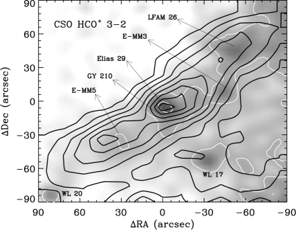
Figure 1: Overlay of IRAM-30m 1.3 mm continuum map (gray scale and two white contours; mott98) and integrated CSO ${\rm HCO^{+}}$ 3-2 emission (black contours) of the Elias 29 region, with source identifications. Contour levels for the continuum map are at the 7, and 14 $\sigma$ confidence level, with $\sigma$ = 10 mJy/15${}^{\prime\prime}$ beam, and $\int T_{\rm MB}~{}dv$ = 1.1, 1.6, …, 4.6 K.${\rm km~{}s^{-1}}$ for ${\rm HCO^{+}}$ 3-2 ($\sigma$ = 0.2 K.${\rm km~{}s^{-1}}$). The 1.3 mm map was aligned to the radio continuum positions of Elias 29 and WL 20. The ${\rm HCO^{+}}$ map in turn was aligned to the 1.3 mm map, for which a small shift of 5″ to the southwest was needed.

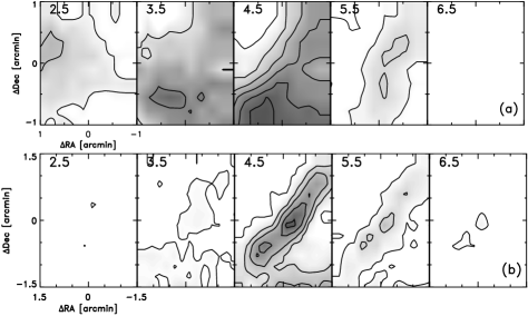
Figure 2: Channel maps of ${\rm C^{18}O}$ 2-1 (a) and ${\rm HCO^{+}}$ 3-2 (b) emission in the Elias 29 region, observed with the CSO telescope. The emission is integrated over a 1 ${\rm km~{}s^{-1}}$ interval, with the central velocity (in ${\rm km~{}s^{-1}}$) indicated in the upper left corners. The contour levels are equally spaced $\int T_{\rm MB}~{}dv$ = 0.8,2.1,…9.9 K.${\rm km~{}s^{-1}}$ for ${\rm C^{18}O}$ ($\sigma=0.20$ K.${\rm km~{}s^{-1}}$), and 0.3, 0.9, …, 2.7 K.${\rm km~{}s^{-1}}$ for ${\rm HCO^{+}}$ ($\sigma=0.09$ K.${\rm km~{}s^{-1}}$). Note that the map scale is 2$\times$2 arcmin for ${\rm C^{18}O}$, and 3$\times$3 arcmin for ${\rm HCO^{+}}$. Foreground clouds are seen in ${\rm C^{18}O}$ 2-1 at 2.5 and 3.7 ${\rm km~{}s^{-1}}$. The Elias 29 core and surrounding ridge are seen at higher velocities, especially in ${\rm HCO^{+}}$.

The ${\rm HCO^{+}}$ 3-2 emission, tracing high densities ($\geq 10^{5}$ ${\rm cm^{-3}}$), is concentrated in a remarkable ridge-like structure, oriented in the southeast-northwest direction (Fig. 1), at a velocity of $V_{\rm LSR}$$\sim$5.0 ${\rm km~{}s^{-1}}$ (Fig. 2). It is likely no coincidence that the protostars Elias 29, WL 20, LFAM 26, GY 210 as well as the 1.3 mm continuum protostellar condensations E-MM3 and E-MM5 are all located along this dense ridge (Fig. 1). The ridge is also particularly prominent in the 800 ${\rm\mu m}$ continuum (john00b). Star formation along dense filamentary structures is common in the $\rho$ Oph cloud, and has been explained by the presence of magnetic field tubes or, more likely, by externally induced shocks (see mott98 for a short discussion).

The ${\rm C^{18}O}$ 2-1 emission, a column rather than volume density tracer, shows that at least three clouds are present along the line of sight of Elias 29 (Fig. 2). The channel maps show a cloud at $V_{\rm LSR}$$\sim 2.7$ ${\rm km~{}s^{-1}}$ that peaks to the northeast of Elias 29, and a cloud at $V_{\rm LSR}$$\sim 3.8$ ${\rm km~{}s^{-1}}$ spread rather evenly over the map. The brightest cloud at $\sim$5 ${\rm km~{}s^{-1}}$ peaks prominently near the south-southwest of the map, and is probably that in which the dense ${\rm HCO^{+}}$ ridge resides, given the similar velocities. All these clouds are likely present in the foreground, since absorption in the ${\rm{}^{12}CO}$ emission lines is seen at these velocities (Fig. 3).

Figure 3: Emission lines of CO, CS, ${\rm HCO^{+}}$, ${\rm H_{2}CO}$, and ${\rm CH_{3}OH}$ toward Elias 29. Vertical dashed lines indicate different dynamic components at $V_{\rm LSR}$=2.7, 3.8 and 5.0 ${\rm km~{}s^{-1}}$. The spectra have been arbitrarily scaled and shifted along the intensity axis. See Table 3 for line intensities.

Table 3: Rotational Transitions Observed toward Elias 29 (Center Position) with Single Dish Telescopes

Molecule	Transition	Frequency	$T_{\rm MB}$	$\int T_{\rm MB}~{}dv$	FWHM	$V_{\rm LSR}$	Beam $\varnothing$	Telescope	Date
		MHz	K	K.${\rm km~{}s^{-1}}$	${\rm km~{}s^{-1}}$	${\rm km~{}s^{-1}}$	arcsec
CO	2-1	230538.0	15.9	19.4	6	2/6.5	21	JCMT	03/1997
	3-2	345796.0	26	98	7	2/6.5	14	JCMT	02/1996
			9	46	6	2/6.5	21	CSO	07/2000
	6-5	691473.0	17	124	12	1.8/6.5	7	JCMT	04/1995
${}^{13}$CO	6-5	661067.4	10	39	3.6	4.78	7	JCMT	04/1995
C${}^{17}$O	1-0 triplet	112358.7	0.40	0.99	2.3	$\cdots$	56	NRAO	05/1995
		112359.0	0.94	1.00	1.0	3.58		NRAO	05/1995
		112360.0	0.68	1.05	1.5	$\cdots$		NRAO	05/1995
	2-1 multiplet	224714.3	1.76	4.95	2.63	4.08	22	JCMT	03/1995
C${}^{18}$O	1-0	109782.2	6.34	11.0	2.0	3.6	57	NRAO	05/1995
	2-1	219560.4	5.81	16.2	2.62	4.19	22	JCMT	03/1995
			9.6	21.3	2.41	4.05	35	CSO	01/2001
	3-2	329330.6	4.3	10.4	2.28	4.24	15	JCMT	02/1996
CS	2-1	97981.0	1.28	3.55	2.61	3.96	64	NRAO	05/1995
	5-4	244935.6	0.56	0.94	1.56	4.92	20	JCMT	03/1995
	7-6	342883.0	$<$0.09	$<0.13$	$\cdots$	$\cdots$	14	JCMT	02/1996
C${}^{34}$S	2-1	96412.9	0.14	0.23	1.62	3.29	65	NRAO	05/1995
H${}_{2}$CO para	$1_{01}-0_{00}$	72838.0	0.62	1.44	2.19	3.80/5.39	86	NRAO	05/1995
	$2_{02}-1_{01}$	145603.0	0.56	0.89	2.0	3.67/4.10	43	NRAO	05/1995
	$3_{03}-2_{02}$	218222.2	0.39	0.66	1.89	4.60	22	JCMT	03/1995
	$3_{22}-2_{21}$	218475.6	$<$0.06	$\cdots$	$\cdots$	$\cdots$	22	JCMT	03/1995
H${}_{2}$CO ortho	$2_{12}-1_{11}$	140839.5	0.80	1.85	2.17	4.20	45	NRAO	05/1995
	$2_{11}-1_{10}$	150498.4	0.80	1.85	2.17	4.20	42	NRAO	05/1995
	$3_{12}-2_{11}$	225697.8	0.41	0.76	1.76	4.93	21	JCMT	03/1995
			0.26	0.48	1.70	4.51	32	CSO	07/2000
CH${}_{3}$OH	2-1 triplet	96739.4	0.15	0.19	1.24	$\cdots$	65	NRAO	05/1995
		96741.4	0.18	0.33	1.68	3.59		NRAO	05/1995
		96744.6	$<$0.03	$\cdots$	$\cdots$	$\cdots$		NRAO	05/1995
	5-4 multiplet	241802.0	$<$0.05	$\cdots$	$\cdots$	$\cdots$	20	JCMT	03/1997
			$<$0.02	$\cdots$	$\cdots$	$\cdots$	31	CSO	06/2000
${\rm HCO^{+}}$	1-0	89188.5	3.57	5.69	3.3/1.0	4.3/4.7	70	NRAO	05/1995
	3-2	267557.6	1.06	2.7	2.28	4.77	18	JCMT	05/1996
			4.34	4.9	1.05	4.63	28	CSO	06/2000
	4-3	356734.3	0.30	0.80	2.5	4.5	21	CSO	03/1999
H${}^{13}$CO${}^{+}$	1-0	86754.3	0.38	0.36	0.90	4.66	72	NRAO	05/1995
	3-2	260255.5	0.04 (0.02)	0.09 (0.02)	2.15	4.89	29	CSO	03/1999

Table 4: Integrated Intensities of Decomposed Lines at Center Position

Molecule	Transition	$\int T_{\rm MB}~{}dv$ for velocity component$\rm{}^{a}$
		2.7 ${\rm km~{}s^{-1}}$	3.8 ${\rm km~{}s^{-1}}$	5.0 ${\rm km~{}s^{-1}}$
C${}^{18}$O	1-0	1.78	5.18	3.97
	2-1	1.93	4.19	9.50
	3-2	1.00	2.75	6.78
C${}^{17}$O${}^{\rm b}$	1-0	0.66	1.94	$<$ 1.6
CS	2-1	0.69	1.01	1.72
	5-4	$<$ 0.07	$<$ 0.09	0.82
	7-6	$<0.13$	$<0.13$	$<$ 0.13
C${}^{34}$S	2-1	0.09	0.12	$<$ 0.05
H${}_{2}$CO para	$1_{01}-0_{00}$	$<0.15$	0.55	0.65
	$2_{02}-1_{01}$	$<$ 0.07	0.43	0.39
	$3_{03}-2_{02}$	$<0.03$	$<0.04$	0.82
	$3_{22}-2_{21}$	$<0.03$	$<0.04$	$<0.12$
H${}_{2}$CO ortho	$2_{12}-1_{11}$	0.30	0.50	1.03
	$2_{11}-1_{10}$	0.21	0.52	0.65
	$3_{12}-2_{11}$	$<0.06$	$<$ 0.09	0.78
CH${}_{3}$OH	2-1 96739.4	0.03	0.14	$<$ 0.05
	2-1 96741.4	0.06	0.18	0.10
	2-1 96744.6	$<0.02$	$<0.02$	$<0.05$
${\rm HCO^{+}}$	1-0	0.49	0.46	4.26
	3-2	$<0.04$	$<0.07$	3.17
	4-3	$<0.05$	$<0.08$	0.76
H${}^{13}$CO${}^{+}$	1-0	$<0.02$	0.05	0.33
${}^{\rm a}$ Relative uncertainties are smaller than the error in the absolute calibration (25%)
${}^{\rm b}$ Derived from 112360.0 MHz fine structure line, multiplied by a factor of 3 to correct for emission in other fine structure lines.

In various other single dish lines these clouds show up as discrete emission components (Fig. 3). The 2.7 and 3.8 ${\rm km~{}s^{-1}}$ components are primarily seen in the low-lying transitions of the CS, ${\rm HCO^{+}}$, ${\rm H_{2}CO}$, and ${\rm CH_{3}OH}$ molecules, indicating low densities and temperatures of these extended clouds. The emission at 5.0 ${\rm km~{}s^{-1}}$, identified with the Elias 29 core and ridge, shows up in the high excitation lines.

Given the fact that these emission components have different spatial distributions, their relative intensity also depends on beam size. The ${\rm HCO^{+}}$ 3-2 line is a factor of 4 stronger and a factor of 2 narrower in the CSO data compared to JCMT: the larger CSO beam (28${}^{\prime\prime}$ versus 18${}^{\prime\prime}$; Table 3) picks up more emission from the ridge, which is bright in the west (§3.2). The wide beam NRAO-12m ${\rm HCO^{+}}$ 1-0 and H${}^{13}$CO${}^{+}$ 1-0 spectra have remarkably narrow 5.0 ${\rm km~{}s^{-1}}$ components, originating from the extended ridge. In contrast, the ${\rm H_{2}CO}$ $3_{12}-2_{11}$ line may peak on the Elias 29 core, rather than the ridge. It has the same width in the CSO and JCMT beams, but the CSO spectrum is weaker (Table 3).

We have performed a Gaussian decomposition of the emission lines to separate the foreground clouds from the dense material around Elias 29. The derived relative strength of these blended lines depends sensitively on the assumed line width. The most reasonable solution, based on the ${\rm H_{2}CO}$ and CS lines and the ${\rm C^{18}O}$ map, is to simultaneously fit the peak intensity with three Gaussians, centered on $V_{\rm LSR}$= 2.7, 3.8, and 5.0 ${\rm km~{}s^{-1}}$, with FWHM=0.5, 0.8, and 1.5 ${\rm km~{}s^{-1}}$. When needed, we allow a 30% variation in the FWHM, and 0.20 ${\rm km~{}s^{-1}}$ in $V_{\rm LSR}$. Some of these small variations may be real, but given the complexity of the line profiles and spatial distribution of the various components, we will not seek a physical interpretation for this. The integrated intensities are summarized in Table 4, and the physical conditions are derived from these in §4.

We conclude that when studying individual protostars in the $\rho$ Oph cloud, it must be realized that many different physical components are present within single dish beams of $\sim 15^{\prime\prime}$ or larger. The spatial information of interferometers is essential here.

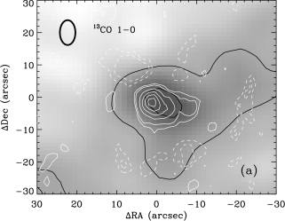
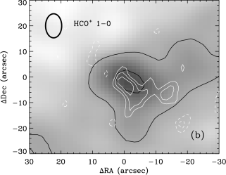
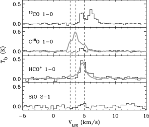
Figure 4: Integrated OVRO ${\rm{}^{13}CO}$ 1-0 (a) and ${\rm HCO^{+}}$ 1-0 (b) emission in the Elias 29 region (white contours), superposed on the 1.3 mm continuum map (gray scale and black contours). Contour levels are drawn at -3,-2, 2, 3, 6, …,15 and -3,-2, 2, 3, and 4 times the noise level (0.48 and 0.90 Jy/beam for ${\rm{}^{13}CO}$ 1-0 and ${\rm HCO^{+}}$ 1-0 resp.). The contours for negative signals are given by white dashed lines. Contour levels for the 1.3 mm map are the same as in Fig. 1. The synthesized beam size is given in the top left corners.

Figure 5: Average line profiles of the central region with more than 2$\sigma$ emission in the OVRO maps, which is an area of 380 arcsec${}^{2}$ for ${\rm{}^{13}CO}$ and 650 arcsec${}^{2}$ for ${\rm HCO^{+}}$. For the non-detected ${\rm C^{18}O}$ and SiO lines we took the central 400 arcsec${}^{2}$. The brightness temperature is correspondingly diluted by factors of 7.4, 5.9, 5.8, and 6.4 from top to bottom respectively to derive the expected signal in the single dish NRAO-12m beam. The smooth gray line for C${}^{18}$O and HCO${}^{+}$ is the NRAO-12m single dish emission, divided by factors of 13 and 9 respectively (for clarity). The vertical dashed lines represent the single dish emission line components shown in Fig. 3.

Figure 6: Channel maps of OVRO ${\rm{}^{13}CO}$ 1-0 (a) and ${\rm HCO^{+}}$ 1-0 (b) emission in the Elias 29 region. The map size is 50${}^{\prime\prime}$. The bullets indicate the map centers, and facilitate comparison of the panels. Contour levels are drawn at -2, 2, 3, 6, 9, 12 (${\rm{}^{13}CO}$) and -2, 2, 3, 4, and 5 times the noise level (0.13 and 0.26 Jy/beam resp.), with the negative contour indicated with dots. Extended emission toward the west is present at velocities near 5.0 ${\rm km~{}s^{-1}}$ in both lines and coincides with the large scale dense ridge seen in our ${\rm HCO^{+}}$ 3-2 single dish map.

3.2 Small Scale Emission: Interferometer Maps

In the OVRO interferometer maps, bright ${\rm{}^{13}CO}$ and ${\rm HCO^{+}}$ 1-0 emission is detected in the direct neighbourhood of Elias 29 (Fig. 6). The ${\rm{}^{13}CO}$ emission is most strongly peaked on the infrared position, and with a spatial FWHM$\sim 6^{\prime\prime}$ (900 AU) it is resolved along the EW direction, where the OVRO beam is smallest (3${}^{\prime\prime}$). This is the Elias 29 core, which likely consists of a disk/envelope system (§4.2). An extension of $\sim 12^{\prime\prime}$ toward the southwest is visible in both lines, but most prominently in ${\rm HCO^{+}}$ 1-0, which must be attributed to the ridge discussed above. Indeed, on this small scale the ${\rm HCO^{+}}$ emission is also parallel to the IRAM-30m 1.3 mm continuum emission (Fig. 6).

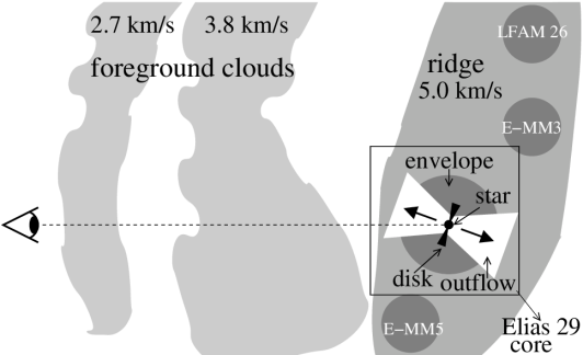
Figure 7: Schematic overview of the proposed geometry of Elias 29 and its environment (not to scale). The line of sight to Elias 29 may cross part of the envelope if the system is slightly more inclined than shown here. Most of the ice-absorption bands originate in the foreground clouds.

The OVRO ${\rm{}^{13}CO}$ and ${\rm HCO^{+}}$ 1-0 spectra peak between $V_{\rm LSR}$=5–7 ${\rm km~{}s^{-1}}$, and show no evidence for the strong, extended 2.7 and 3.8 ${\rm km~{}s^{-1}}$ foreground emission seen in the single dish maps (Fig. 6). The ${\rm C^{18}O}$ 1-0 emission is spectacularly absent in the interferometer spectrum; it is at least a factor of 10 weaker compared to the single dish data. After dilution to the NRAO-12m beam (taking the emitting area from the OVRO ${\rm{}^{13}CO}$ image), the OVRO ${\rm C^{18}O}$ signal is even a factor of 60 weaker than the bright detection with the NRAO-12m telescope. This shows again that the bulk of the molecular material in the Elias 29 line of sight is not associated with Elias 29, but instead is present in extended foreground clouds, which are resolved out by the OVRO interferometer.

It is interesting to note that the OVRO line profiles are double peaked (Fig. 6), with a 5.0 ${\rm km~{}s^{-1}}$ component emitting in the dense ridge (Fig. 6). Emission at the central infrared position is strongest at 6 ${\rm km~{}s^{-1}}$. Whether this is a true dynamical difference between the Elias 29 core and the ridge, or artificially created by self-absorption at $\sim 5.5$ ${\rm km~{}s^{-1}}$, is difficult to answer at present. In this paper we will keep referring to this as the 5.0 ${\rm km~{}s^{-1}}$ component. A disk/envelope/ridge decomposition is attempted in §4.2.

4 Discussion: Physical Conditions

It is our aim to derive the physical structure of the surroundings of Elias 29, and to locate the origin of the ices, seen abundantly along this line of sight (boog00b). In §4.1 the extended clouds at 2.7 and 3.8 km s${}^{-1}$ identified above are discussed; §§4.2 and 4.3 describe the more immediate circumstellar environment of Elias 29 in terms of a near face-on disk, a remnant envelope, and the dense ridge from which the star may have formed (see Fig. 7). The physical conditions in each of the components are constrained using the intensities and intensity ratios of the single dish and interferometer line emission, the 1.3 mm continuum emission (mott98), and the infrared SED (boog00b). This is linked to the ice observations in §4.4.

4.1 Foreground Clouds

The C${}^{18}$O line emission at 2.7 and 3.8 km s${}^{-1}$ is extended over several arcminutes (Fig. 2), and thus is associated with the overall $\rho$ Oph cloud complex. Assuming that the clouds are sufficiently homogeneous, we can use the ratios of the decomposed line intensities (Table 4) to find the density and temperature, and subsequently the column density, in each of the clouds. We use the escape-probability method described by jans95 to calculate the molecular excitation.

The most useful constraints on the density and temperature are given by the intensity ratios of ${\rm C^{18}O}$ 1–0/3–2 and ${\rm HCO^{+}}$ 1–0/3–2. Fig. 4.1 visualizes the density and temperature values allowed by the observed ratios, taking into account line-opacity effects. The 2.7 ${\rm km~{}s^{-1}}$ component has a temperature $T=15\pm 5$ K, and a density $n$(H${}_{2}$)=($1\pm 0.5$) $\times 10^{4}$ ${\rm cm^{-3}}$. For the 3.8 ${\rm km~{}s^{-1}}$ component, the density is less than $10^{5}$ ${\rm cm^{-3}}$, but the temperature cannot be significantly constrained from the line ratios. Here we use the far infrared SED to find that $T_{\rm kin}=25\pm 15$ K (§4.2). Taking a C${}^{18}$O abundance with respect to H${}_{2}$ of $3.6\times 10^{-7}$ ($N$[CO]/$N$[C${}^{18}$O]=560, wils94; $N$[H${}_{2}$]/N[CO]=5000, lacy94), the H${}_{2}$ column densities of the 2.7 and 3.8 km s${}^{-1}$ clouds are $5\times 10^{21}$ cm${}^{-2}$ and $1.4\times 10^{22}$ cm${}^{-2}$, respectively (Table 6). This also assumes that CO is not strongly depleted in these clouds, which is validated in §4.5. These parameters fit the optically thin C${}^{17}$O lines also, indicating that a correct line opacity was used

With these physical parameters at hand, we calculate that the optical depth of the clouds in the CO 5-6 transition is $\sim$4. This is sufficiently high to explain the absorption in the CO 6-5 lines at 2.7 and 3.8 ${\rm km~{}s^{-1}}$ (Fig. 3). The bright CO 6-5 emission is closely associated with Elias 29 (C. Ceccarelli et al., in prep.), and therefore the 2.7 and 3.8 ${\rm km~{}s^{-1}}$ clouds are located in front of this source.

Independent information on the physical conditions in these extended foreground clouds is obtained from the SED longward of 100 ${\rm\mu m}$ (§4.2). The columns and temperatures compare also favorably with the extended cold dust found by sensitive 180–1100 $\mu$m balloon-based measurements (rist99; Table 6).

The observed lines of CS, H${}_{2}$CO, and CH${}_{3}$OH do not further constrain the physical conditions, but they can be used to derive abundances. These are listed in Table 6, and further discussed in §4.5.

Temperature and density range constrained by intensity ratios of ${\rm C^{18}O}$ 1–0/3–2 (thin lines) and HCO${}^{+}$ 1–0/3–2 (thick lines) for the foreground clouds at $V_{\rm LSR}$=2.7 (a) and 3.8 ${\rm km~{}s^{-1}}$ (b), and for the ridge material at 5.0 ${\rm km~{}s^{-1}}$ (c). The intensity ratios for the ridge material have been corrected for the expected contribution from the envelope and disk of Elias 29. The filled star indicates the adopted temperature and density for each of the components.

4.2 The Circumstellar Environment of Elias 29

Understanding the circumstellar environment of Elias 29 requires the combination of several pieces of crucial information: the single-dish ${\rm HCO^{+}}$ 3–2 map and 1.3 mm dust-continuum distribution (Fig. 1), the spatially resolved emission in ${}^{13}$CO 1–0 and ${\rm HCO^{+}}$ 1–0 observed by OVRO (Fig. 6), and the infrared SED obtained by the SWS and LWS spectrometers of the ISO satellite (boog00b; Fig. 8).

The ${\rm HCO^{+}}$ 3–2 and 1.3 mm continuum maps show that Elias 29 is located in a narrow, dense ridge, $\lesssim 30^{\prime\prime}$ wide and several arcminutes long. The strongest ${\rm HCO^{+}}$ 3–2 peak in the ridge is situated near Elias 29. The OVRO images and channel maps (Figs. 6 and 6) show that part of the ${}^{13}$CO and ${\rm HCO^{+}}$ emission is centered on Elias 29, while a significant fraction follows the crest of the ridge, $10^{\prime\prime}$–$20^{\prime\prime}$ offset to the west/southwest. This shows that multiple components are present in the immediate vicinity of Elias 29 (i.e., within a typical single-dish beam), in addition to the multiple velocity components along the line of sight (§4.1). The velocity coincidence between the ridge and Elias 29 further supports that the star formed from the ridge.

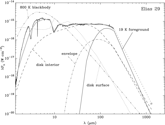
Figure 8: Infrared SED of Elias 29 as observed by ISO LWS and SWS (thin line with ice and silicate absorption features; boog00b) combined with the 1.3 mm flux in the 15″ IRAM-30m beam (open square; mott98). The thick gray line shows the modeled SED as described in §4.2. It consists of four components: (1) a 0.012 M${}_{\odot}$ flared circumstellar disk following chia97 with a two-layer vertical temperature structure (cool interior [long-dashed line] and superheated surface [dotted line]); (2) a 0.12 M${}_{\odot}$ collapsing envelope (dash-dot line); (3) an ad hoc 800 K central blackbody with a 1.4 AU radius (dash-triple dot line), required to fit the flux maximum at $\lambda\sim 5$ ${\rm\mu m}$ and probably corresponding to the warmest regions of the disk close to the star and/or the stellar photosphere extincted by the disk; and (4) a 19 K foreground layer (thin solid line peaking at $\sim$120 ${\rm\mu m}$) with a column density of $N({\rm H_{2}})=1.9\times 10^{22}$ cm${}^{-2}$ as derived for the material at $V_{\rm LSR}$=2.7 and 3.8 ${\rm km~{}s^{-1}}$ in §4.1, which is responsible for the continuum absorption below 3 ${\rm\mu m}$ in the final four component model, and for the prominent silicate and ice absorption bands.

4.2.1 SED and Continuum Modeling

The most important clues about the nature of Elias 29 are offered by the infrared SED. Because of the large beam with which these measurements were taken (§2), the SED reflects not only Elias 29 but also many of the other components identified above. Our ability to derive accurate parameters for each component therefore proved essential in helping to understand the nature of Elias 29. The SED (Fig. 8) is remarkably flat between 10 and 200 $\mu$m. At 10 $\mu$m there is a prominent silicate absorption band, and at 5 $\mu$m the SED shows a broad peak on top of which a number of sharp ice absorption features are present. Below 2 $\mu$m the emission drops off sharply. Flat protostellar SEDs are generally explained by a circumstellar disk. Compared to other circumstellar material distributions, a disk, especially a flared one, has the surface-area vs. temperature distribution required to create a flat SED.

For our analysis, we adopt the flared disk model of chia97 with the parameters listed in Table 7. The flatness of the SED is explained in this model by a superheated surface layer. The continuum emission of the disk is modeled using the radiative transfer part of the Monte-Carlo code of hoge00; this part of the code simply calculates the expected continuum emission from a given distribution of density and temperature by building up a grid of points on the sky, for each of which the radiative transfer is solved along straight lines. The resulting grid is then convolved with the appropriate beam sizes. Because of the large number of parameters involved, their values should be considered as representative only. We believe that the general characteristics of the model are firmly established, however. The flatness of the SED over a large wavelength range (4-100 ${\rm\mu m}$; Fig. 8) limits the inclination of the system to $<60^{\circ}$ ($90^{\circ}$ being edge-on; chia99). Such a low inclination cannot explain the deep ice and silicate absorption features that are visible in the observed SED; these must originate in the envelope and foreground clouds. The low disk inclination is compatible with the very high velocity ($\sim 80$ ${\rm km~{}s^{-1}}$), variable outflowing hot CO gas seen in this object (A.C.A. Boogert, G.A. Blake, & M.R. Hogerheijde, in prep.). A fully face on orientation is however not likely, given the presence of low surface brightness scattered K band light out to distances of 15${}^{\prime\prime}$ (2400 AU) from the central object (Zinnecker, Perrier, & Chelli 1988). This light presumably traces the outflow lobes, adjacent to the remnant envelope and the outer edges of the disk. The emission is extended along the southwest/northeast direction, perpendicular to the high velocity outflowing gas (C. Ceccarelli et al., in prep.), with an axis ratio compatible with an inclination of roughly $\rm\sim 30^{o}$. Flattening on a similar scale is observed in the OVRO images and in the 1.3 mm continuum IRAM-30m single dish map.

Table 5: Physical Conditions in Elias 29 Foreground Clouds and Ridge, and Comparison with Other Clouds

Quantity	Unit	Cloud component			TMC 1${}^{d}$	NGC 1333${}^{e}$
		2.7 ${\rm km~{}s^{-1}}$	3.8 ${\rm km~{}s^{-1}}$	5.0 ${\rm km~{}s^{-1}}$		IRAS 4A	IRAS 4B
$b_{\rm D}$	[${\rm km~{}s^{-1}}$]	0.3	0.5	1.0	$\cdots$	$\cdots$	$\cdots$
$T_{\rm kin}$	[K]	15 (5)	25 (15)	15 (5)	$\cdots$	$\cdots$	$\cdots$
$n{\rm(H_{2})}$	[10${}^{4}$ ${\rm cm^{-3}}$]	1.0 (0.5)	$<10$	40 (20)	$\cdots$	$\cdots$	$\cdots$
$N{\rm(H_{2})}$	[10${}^{22}$ ${\rm cm^{-2}}$]	0.5 (0.2)	1.4 (0.2)	1.0 (0.2)	1.0	14	6
$X$(${\rm C^{18}O}$)${}^{a}$	[10${}^{-9}$]	360	360	360	304	40	70
$X$(C${}^{17}$O)${}^{a}$	[10${}^{-9}$]	110	110	110	95	7.6	19
$X$(CS)	[10${}^{-9}$]	6.0	15.0	$\cdots$ ${}^{b}$	6	1.2	0.2
$X$(${\rm HCO^{+}}$)	[10${}^{-9}$]	0.6	0.7	$\cdots$ ${}^{b}$	9	0.4	0.1
$X$(ortho ${\rm H_{2}CO}$)	[10${}^{-9}$]	3.0	8.0	$\cdots$ ${}^{b}$	50	0.4	0.9
$X$(para ${\rm H_{2}CO}$)	[10${}^{-9}$]	$<$1.0	2.7	$\cdots$ ${}^{b}$	$\cdots$	$\cdots$	$\cdots$
$X$(${\rm CH_{3}OH}$)	[10${}^{-9}$]	0.4	0.5	$\cdots$ ${}^{b}$	3	$\cdots$	$\cdots$
$A_{\rm V}$	[mag]	2.9	8.2	$<5.9^{c}$	$\cdots$	$\cdots$	$\cdots$
General: all abundances $X$ are w.r.t. H${}_{2}$ and have an error of 50%
${}^{\rm a}$ From H${}_{2}$ using standard relations (see text), except TMC-1
${}^{\rm b}$ Line intensities in ridge have to be corrected for expected contribution from envelope and disk (see text). No independent determination of abundances is therefore possible.
${}^{\rm c}$ Upper limit; only a fraction of the ridge material may actually be in front of Elias 29.
${}^{\rm d}$ on ‘CP’ peak; prat97; ohis98
${}^{\rm e}$ blak95, assuming $N({\rm H_{2}})$ from dust

Table 6: Column Density of Cold Gas Derived by Different Methods

Method	Component	$N{\rm(H_{2})}$$\rm{}^{a}$	$A_{\rm V}$$\rm{}^{b}$
		10${}^{22}$${\rm cm^{-2}}$
silicate absorption$\rm{}^{c}$		2.5-6	14-34
4.7 ${\rm\mu m}$ ${\rm{}^{13}CO}$ absorption$\rm{}^{d}$	$b_{\rm D}$=1.0 ${\rm km~{}s^{-1}}$	3 (0.5)	17 (3)
	$b_{\rm D}$=0.7 ${\rm km~{}s^{-1}}$	11 (4)	63 (23)
${\rm C^{18}O}$ 2-1 emission	$V_{\rm LSR}$=2.7	0.5 (0.2)	2.9 (1.1)
	$V_{\rm LSR}$=3.8	1.4 (0.2)	8.0 (1.1)
	$V_{\rm LSR}$=5.0	1.0 (0.2)	5.7 (1.1)
ISO SED and IRAM-30m 1.3 mm	envelope	0.3-1	1.7-6
0.18–1.1 mm continuum$\rm{}^{e}$	10–15 K	0.5–5	2.9-29
X rays$\rm{}^{f}$		3.8	22
$\rm{}^{a}$ assuming $N{\rm(H_{2})}/N{\rm(CO)}=5\times 10^{3}$; $\rm{}^{b}$ conversion factor $A_{\rm V}=N{\rm(H_{2})}\times 8.6/15\times 10^{21}$ bohl78; $\rm{}^{c}$ see boog00b; $\rm{}^{d}$ A.C.A. Boogert et al., in preparation; $\rm{}^{e}$ Balloon experiment: rist99; $\rm{}^{f}$ iman01

The flux between 20 and 40 $\mu$m indicates a temperature scaled upward by a factor of 2.25 with respect to the values used by chia97. The central star is therefore approximately 50 times brighter than their standard model, presumably because it has a higher mass (using the scaling relation $T\propto L^{1/5}$; chan00). The disk midplane dominates the emission beyond 25 $\mu$m, and the shape of the SED at these wavelengths limits the disk radius to $\sim$ 500 AU. The warmer surface layer dominates the shorter wavelengths and generate a silicate emission feature at 10 $\mu$m (Fig. 8). The disk model can explain only $\sim$20% of the emission maximum around 5 $\mu$m. Indeed, speckle observations of Elias 29 reveal the presence of a $\sim$400 AU radius thermally emitting region ($T$ a few 100 K; i.e. not scattered light) responsible for $\sim$20% of the M band flux (zinn88), which, in our model, is explained by the warm disk surface layer. The observed remaining 80% of the M band emission originates from hot dust within a few AU from the central object. Perhaps this is a puffed up hot rim at the inner disk edge, just outside the region where dust has evaporated ($T_{\rm subl}\sim 1500$ K; dull01; zinn88). The innermost, hottest, part of the rim may be related to the 0.25 AU radius structure found in lunar occultation K band observations (simo87). We do not attempt to fit the inner regions and stellar photosphere with that level of detail, but instead use an 800 K blackbody with an effective radius of 1.4 AU to explain the remaining 80% of M band emission, and roughly the shape of the SED at shorter wavelengths (Fig. 8).

The disk alone is also insufficient to explain the emission beyond $\sim 55$ $\mu$m. The single-dish line emission clearly reveals the presence of appreciable columns of material at 2.7 and 3.8 km s${}^{-1}$ (§4.1). When filling the ISO beam with these columns, the emission between 55 and 180 $\mu$m can be fit at a dust temperature of 19 K. This material provides sufficient opacity in the 10 ${\rm\mu m}$ silicate band to turn the disk’s emission feature into the observed absorption feature. The opacity shortward of 2 $\mu$m is also sufficient to explain the observed steep drop in emission at short wavelengths. This strongly suggests that a large fraction of the 2.7 and 3.8 km s${}^{-1}$ material is located in front of Elias 29, as was found from the absorption in the ${\rm{}^{12}CO}$ emission lines as well (§4.1).

Table 7: Parameters of Disk and Envelope Model

Item	Value
Disk: chia97
Temperature	$2.25\times$ standard model of Chiang & Goldreich
Dust opacity	osse94, MRN model with $10^{6}$ years of coagulation at $10^{5}$ cm${}^{-3}$
Inner radius	0.01 AU
Outer radius	500 AU
Mass	0.012 M${}_{\odot}$
% mass in superheated surface layer	2.5%
Envelope: shu77
Sound speed	0.13 km s${}^{-1}$
Age	$2.2\times 10^{5}$ yr
Radius of collapse expansion wave	6000 AU
Temperature	$35\,(r/1000\,{\rm AU})^{-0.4}$ K
Dust opacity	osse94, MRN model with $10^{6}$ years of coagulation at $10^{5}$ cm${}^{-3}$
Inner radius	500 AU (3″)
Outer radius	6000 AU (39″)
Mass	0.12 M${}_{\odot}$

Radial intensity profile along the ridge centered on Elias 29 obtained from the 1.3 mm map of mott98 (bullets with error bars), compared to the predicted profile based on a model for Elias 29 with a disk and an envelope (solid line) and with a disk only (dashed line). Both models include a 19 K, $N({\rm H_{2}})=6\times 10^{21}$ cm${}^{-2}$ background to fit the levelling off of the emission beyond a radius of $25-50^{\prime\prime}$. Note that the true total background column, filtered out of the IRAM-30m 1.3 mm data, is a factor of 3 higher (§4.2.1).