Implications of a solar-system population of massive 4th generation neutrinos

for underground searches of monochromatic neutrino-annihilation signals.

K.M. Belotsky¹, T. Damour², and M.Yu. Khlopov^1,2

¹ Center for Cosmoparticle Physics "Cosmion",

125047, Moscow, Russia

² Institut des Hautes Etudes Scientifiques,

91440, Bures-sur-Yvette, France

Abstract

It has been recently pointed out that any primary galactic population of Weakly Interacting Massive Particles (WIMP) generates, through collisions with solar matter, a secondary population of “slow” WIMPs trapped in the inner solar system. We show that taking into account this “slow” solar-system population dramatically enhances the possibility to probe the existence of stable massive neutrinos (of a 4th generation) in underground neutrino experiments. Though neutrinos, with mass in the 45-90 GeV range, can only represent a sparse subdominant component of galactic cold dark matter, a combination of enhancement factors makes it possible to discriminate their contribution to WIMP annihilation effects in the Earth. Our work suggests that a reanalysis of existing underground neutrino data should be able to bring extremely tight constraints on the possible existence of a stable massive 4th neutrino.

1 Introduction

The total number of quark-lepton families is not known for sure. Experimentally, three generations have been found at present. Theoretically, the number of generations could be larger. In superstring-inspired particle models the number of generations is defined by some topological characteristics of the manifold of compactified additional dimensions, and any number of generations is a priori possible [1].

Another important prediction of almost all realistic superstring-inspired models is the existence of at least one additional $U(1)$ gauge group in the low energy limit of the theory. Recently [2] it was suggested to ascribe such a new $U(1)$ gauge group to an additional, fourth, fermion generation only. In this case the new gauge group can remain unbroken. Such an unbroken $U(1)$ gauge group implies the existence of a strictly conserved charge, which, in turn, accounts for the stability of the lightest particle of the 4th generation, and forbids any mixing with the other (usual) three generations. It will be assumed that the lightest particle of the 4th generation is its neutrino.

The direct search for new generation fermions on accelerators leads to a lower bound on their masses in the range 50-100 GeV. The mass of a 4th generation neutrino $m_{\nu}$ is restricted by the measurement of the width of the Z-boson to $m_{\nu}>m_{Z}/2\approx 45$ GeV if it is a (quasi)stable Dirac neutrino (for a Majorana one the restriction is slightly lower; for an unstable one the lower limit is about 90 GeV). Another possibility to search for a fourth generation neutrino, with mass $m_{\nu}>m_{Z}/2\approx 45$ GeV, at accelerators was suggested in [2], [3]. A detailed analysis of the data on the parameters of the Standard Model, accounting for the possible contributions of virtual new generation fermions, allows for the existence of an additional generation if the mass of the new (fourth) neutrino is about 50 GeV [4] and if the masses of the other fermions of the new generation exceed 100 GeV.

The existence of new generation fermions in the Universe can lead to many observable astrophysical effects. This makes the appropriate cosmological and astrophysical analysis an important tool for probing the possible existence and properties of such 4th generation fermions. In particular, a new neutrino, being plausibly the lightest of its generation, and thus possibly stable, is of the most interest in such an analysis.

As was found long ago [5], the existence of a heavy Dirac neutrino is compatible with the upper limit on the total density of the Universe if its mass exceeds 2 GeV. Indeed, for a neutrino mass greater than 3 MeV, neutrino annihilation through weak interactions reduces their cosmological concentration at freeze out. A larger neutrino mass corresponds to a larger annihilation cross section, and therefore to a smaller relic heavy neutrino density $\Omega_{\nu}=\rho_{\nu}/\rho_{critical}$ (see Fig.2 below). Moreover, if $m_{\nu}=m_{Z}/2$ the Z-boson annihilation resonance leads to a dip in the relic density. For instance, if $m_{\nu}=50$ GeV, close to the Z-boson resonance dip, $\Omega_{\nu}\approx 10^{-4}$. Such a rare population of neutrinos does not play any significant dynamical cosmological role as a Cold Dark Matter (CDM) contributor. Nevertheless a more refined astrophysical analysis [2], [6] showed that the effects of such rare, massive neutrinos can be accessible to some experimental searches and/or astrophysical observations. In the present paper, we shall mainly consider the mass range $45<m_{\nu}<90$ GeV, corresponding to such a sparse population of heavy neutrinos.

Heavy neutrinos, as any form of CDM, must be concentrated in galaxies. The ratio of galactic neutrino density to the mean cosmological density is a model-dependent parameter (denoted here as $\xi$) which is strongly sensitive to the details of galactic halo formation. In this work we shall assume that the concentration factor $\xi$ is the same for massive neutrinos and for the dominant contributor to CDM. It is usual to estimate $\xi$ by taking the ratio between a local (i.e, in the vicinity of the Solar system) density of CDM equal to $0.3\,\rm{GeV/cm^{-3}}$, and a mean cosmological density corresponding to $\Omega_{CDM}=0.3$. This leads to the “standard” estimate: $\xi=2\times 10^{5}$. In most of this paper, we shall assume this standard value (except, when explicitly said otherwize).

In previous papers [2], [6] we already analyzed several astrophysical consequences of such a sparse galactic population of heavy neutrinos. In particular we studied [7] the (ordinary) neutrino fluxes emitted by the annihilation of heavy neutrino-antineutrino pairs accumulated in the core of the Earth. [Such an accumulation takes place for many types of weakly interacting massive particles (WIMP) [8].]

Recently, it was pointed out [9] that this annihilation flux can be strongly enhanced by the existence of a “slow” Solar-system population of WIMP’s, trapped in the gravitational field of the Solar system by an initial inelastic interaction with the Sun [10]. The aim of the present paper is to analyze in detail, in the case of a heavy neutrino WIMP, the density of this new “slow” Solar-system population, and its enhancement effect on the annihilation flux from the core of the Earth. We shall show that the existence of the slow population qualitatively improves the sensitivity of underground neutrino data to the effects of 4th neutrino annihilation, and makes these data a significant probe of the existence of a 4th neutrino.

2 Number density of the “slow” heavy neutrino population

Let us recall (from [10]) that the “slow” population of WIMPs is generated by inelastic collisions of incident primary (“fast”) galactic WIMPs with nuclei in the outer layers of the Sun. A fraction of these WIMPs are scattered, by the collision, on orbits that “graze” the surface of the Sun, and which evolve, under the subsequent perturbing gravitational influence of planets, onto orbits that do not penetrate the Sun. This allows these WIMPs to survive for a long time in the Solar system. This population has a much lower typical velocity ($\sim$30 km/sec) than the incident galactic one. This fact amplifies the probability of their capture by the Earth (we will further refer to this population as “the slow component”). The number density (in the vicinity of the Earth) of this slow component of heavy neutrinos, $n_{slow}$, has been derived in Ref.[10] and reads:

$$n_{slow}=\frac{0.212}{v_{0}/220\,\rm{km/s}}g_{tot}^{(-10)}\times n_{gal},$$ (1)

$$g_{tot}^{(-10)}=10^{10}\times\sum\limits_{A}\frac{f_{A}}{m_{A}}\sigma_{A}K_{A}^{s}\,(\rm{GeV^{3}}),$$

$$K_{A}^{s}=\frac{v_{0}}{\beta_{+}}\int_{0}^{v_{max}}4\pi v_{\infty}dv_{\infty}f(v_{\infty})F^{2}(v_{\infty}).$$

Here $f(v_{\infty})$ is the angular average of the velocity distribution of galactic WIMPs. [Our notation differs slightly from Ref. [10] in that we factor out the number density $n_{gal}$ from the phase-space distribution function, and delete the bar over $f(v_{\infty})$ indicating the angular average.] The parameter $v_{0}$ is the characteristic velocity entering the (assumed) Maxwellian velocity distribution $f(v_{\infty})$. Throughout the paper the index $\infty$ refers to quantities far from the Sun or (depending on the context) the Earth. The meaning of the other quantities entering the equations above is: $m_{A}$ is the mass of the nucleus $A$, $f_{A}$ denotes its mass fraction in the Sun, $\sigma_{A}$ is the cross-section of neutrino-nucleus scattering in the point-like approximation. The form-factor $F(v_{\infty})$ takes into account the effect linked to the extension of the nucleus. More about cross-section and form-factor below. The quantity $g_{tot}$ (which has dimensions $[crosssection]\times[mass]^{-1}$ should be expressed in GeV³. Here and below we use the notation

$$\beta_{\pm}=\frac{4m_{\nu}m_{A}}{(m_{\nu}\pm m_{A})^{2}},$$ (2)

$m_{\nu}$ denoting the neutrino mass. The upper limit, $v_{\max}$, of the integral above comes from kinematics and is read from Eq.(2.16) of [10]

$$v_{\max}=\frac{\sqrt{4m_{\nu}m_{A}v_{esc}^{2}(\bar{R}_{S})-(m_{\nu}+m_{A})^{2}\alpha}}{\left|m_{\nu}-m_{A}\right|},$$ (3)

in which we used the following numerical estimates:

$$v_{esc}^{2}(\bar{R}_{S}=0.907R_{S})=(644\,\rm{km/s})^{2},$$ (4)

where $R_{S}$ denotes the Solar radius, and $\alpha=GM_{S}/a\simeq(30\,\rm{km/s})^{2}$, $a$ denoting the semi-major axis of the WIMP orbit. As said above, we take a WIMP velocity distribution (far from the Sun) which is Maxwellian, i.e. (after angular averaging)

$$f(v)=\frac{1}{4\sqrt{\pi^{3}}v_{0}v_{S}v}\left(\exp\left(-\frac{(v-v_{S})^{2}}{v_{0}^{2}}\right)-\exp\left(-\frac{(v+v_{S})^{2}}{v_{0}^{2}}\right)\right).$$ (5)

Here $v_{S}$ denotes the velocity of the Sun relative to the gas of galactic neutrinos. In the estimates below, we took $v_{S}=200$ km/s. We also estimated the effect of varying $v_{S}$ between zero and $200$ km/s and found that it changed only insignificantly the results given below. The parameter $v_{0}$ denotes the characteristic velocity dispersion of the Maxwell distribution (i.e. it measures the “temperature” of this distribution). In our estimates below we shall use the value $v_{0}=220$ km/s. For comparison, we shall also mention the results for $v_{0}=266$ km/s, which corresponds to a mean velocity of 300 km/s.

The data about the chemical composition of Solar matter was taken as in Ref. [10] (i.e., a combination of the values given in [11] and [12]). We also follow Ref. [10] in taking nuclei form-factor of the form:

$$F^{2}(v)=\exp\left(-\frac{Q(v)}{Q_{A}}\right),$$ (6)

where $Q=\frac{m_{\nu}(v^{2}+\alpha)}{2}$ is the transferred energy from neutrino to nucleus, $Q_{A}=\frac{3\hbar^{2}}{2m_{A}R_{A}^{2}}$, $R_{A}=10^{-13}\,{\rm cm}\,(0.3+0.91(\frac{m_{A}}{\rm{GeV}})^{1/3})$.

The total $\nu-A$ cross-section for a point-like nucleus $\sigma_{A}$ is approximated by a purely spin independent coupling, except in the case of hydrogen. Since most contributing nuclei have a first excited energetic level higher than the characteristic energy tranfer $Q$ the collision is assumed to be elastic. This leads to a cross-section of the form

$$\sigma_{A}=\frac{G_{F}^{2}}{8\pi}\frac{m_{\nu}^{2}m_{A}^{2}}{(m_{\nu}+m_{A})^{2}}\left(F_{V}^{2}+3F_{A}^{2}\delta_{A}^{1}\right),$$ (7)

where $G_{F}$ is the Fermi constant, $F_{V}=-(A-2(1-2\sin^{2}\theta_{W})Z)$ is the vector form-factor (all $q^{2}$-dependence is taken out into $F(v)$), $\theta_{W}$ is the Weinberg angle, and $F_{A}$ is the axial form-factor, which is taken into account only in the case of hydrogen (hence the Kronecker symbol $\delta_{A}^{1}$).

After substituting all these quantities in Eq. (1) we obtain the dependence on $m_{\nu}$ of the density enhancement ratio $\delta_{E}=\frac{n_{slow}}{n_{gal}}$ showed in Fig.1. In Table 1, we fix $m_{\nu}=50$ GeV, and study the sensitivity of the density enhancement $\delta_{E}$ to the choices of the two velocity parameters entering our study: $v_{0}$ and $v_{S}$.

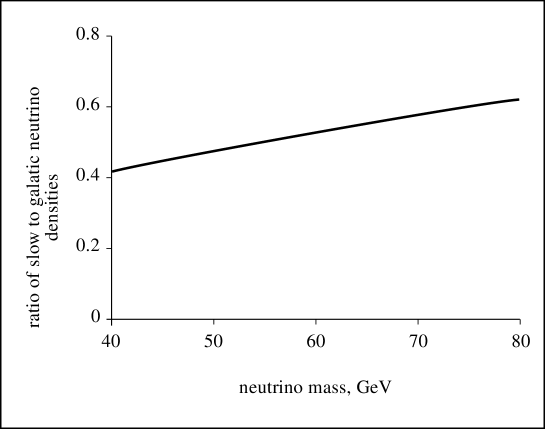
Figure 1: Density enhancement $\delta_{E}=n_{slow}/n_{gal}$ as a function of the neutrino mass $m_{\nu}$.

	$v_{0}=220\,\rm{km/s}$	$v_{0}=266\,\rm{km/s}$
$v_{S}=0$	0.728	0.529
$v_{S}=200\,\rm{km/s}$	0.475	0.388

Table 1: Density enhancement $\delta_{E}=n_{slow}/n_{gal}$ for different velocity parameters.

The crucial new result to note from Fig. 1 and Table 1 is that, contrary to the case of a generic neutralino WIMP where the density enhancement (near the Earth) due to the slow population, $\delta_{E}=n_{slow}/n_{gal}$, was typically of the order of a few percent, here this density enhancement is of the order of 50 %. This shows that it is crucial to take into account the existence of the slow population to estimate the detectability of a 4th neutrino . In addition to this significant enhancement in the local density of WIMPs, we turn now to the estimate of the capture rate of the WIMPs by the Earth which is further amplified by the fact that slow WIMPs (with velocity $\sim 30$ km/s) are much more easily captured by the Earth gravitational field than galactic ones (with velocity $\sim 220$ km/s).

3 Capture rate of massive neutrinos by the Earth

The neutrinos interacting with the Earth matter can be captured by the Earth gravitational potential well if they lose enough energy in the collision with a nucleus in the Earth. The “slow” neutrinos, having an incident velocity already comparable with the escape velocity from the Earth ( $v^{esc}_{E}\sim 10\,\rm{km/s}$), have a much greater probability to be captured than galactic ones. It is therefore quite important to take their effect into account.

Among all nuclei present in the Earth the iron nuclei play the main role in the capture process for the neutrino mass range ( $45\,\rm{GeV}<m_{\nu}<90\,\rm{GeV}$) that interests us.

The capture rate of WIMPs by the Earth has been studied in detail by Gould [13] (see also [9]). In the present study, we estimated the capture rate by starting from Eq.(5.7) and Eq.(5.8) of [9], and by approximating the result in the following way. We replaced the integrals over the volume of the Earth of the type $\int d^{3}x\,n_{A}(r)f(r)$ by $N_{A}\langle f(r)\rangle$, where $N_{A}$ is the total number of nuclei of type $A$, and where $\langle f(r)\rangle$ is a suitable (approximate) average of $f(r)$. Actually, we consider only the capture by iron. As iron is concentrated in the core of the Earth we can use the average of the squared escape velocity given in [13]: $\langle v_{esc}^{2}\rangle=1.6\times(11.2\,\rm{km/s})^{2}$. We assume that the fraction of the mass of the Earth in iron is 20 %. Finally, our simplified capture rate reads:

$$R_{cap}=\frac{2Q_{Fe}}{\beta_{-}m_{\nu}}N_{Fe}\sigma_{Fe}\int_{0}^{\sqrt{\beta_{-}\langle v_{esc}^{2}\rangle}}\frac{dn_{\nu}}{v}\times$$

$$\times\left[\exp\left(-\frac{m_{\nu}}{2Q_{Fe}}v^{2}\right)-\exp\left(-\frac{m_{\nu}}{2Q_{Fe}}\beta_{+}(\langle v_{esc}^{2}\rangle+v^{2})\right)\right]$$ (8)

The neutrino distribution function $dn_{\nu}$ to be inserted in Eq.(8) depends on whether we consider galactic or slow neutrinos. For galactic neutrinos it is $dn_{gal}=n_{gal}\,f(v)d^{3}v$. For slow neutrinos we followed Eq.(3.15) of [9] (with $\lambda=1$ ; $\varepsilon=0.18377$), i.e, explicitly,

$$dn_{slow}=n_{slow}\,f_{slow}(v_{slow})dv_{slow}=n_{slow}\,Cv\frac{\theta(1.617\times v_{E}-v)}{(3\times v_{E}^{2}-v^{2})^{0.6}}\times$$

$$\times\left(\sqrt{v^{2}-0.816\times v_{E}^{2}}\,\theta(v-0.904\times v_{E})-\sqrt{v^{2}-1.184\times v_{E}^{2}}\,\theta(v-1.089\times v_{E})\right)dv\,,$$ (9)

where $C=91.775^{-1}$ is a normalization factor, $\theta(x)$ is the step function, $v_{E}=30\,$km/s is the velocity of the Earth orbital motion, and where $n_{slow}$ is given by Eq.(1) above.

Another crucial parameter for our problem is the value of the incident galactic neutrino number density itself. Contrary to the case usually considered for WIMP capture, we cannot assume here that the sparse 4th neutrino population is the principal constituent of Cold Dark Matter, i.e we cannot assume that its galactic density has the “standard” value $\rho_{CDM}\sim 0.3\,\rm{GeV/cm^{3}}$. Instead, we need to estimate what is the relic density of 4th neutrinos left over from the Big Bang, and to multiply it by an estimate of the typical density enhancement, in a galaxy. We can then write the galactic neutrino number density (as a function of the neutrino mass) as:

$$n(m_{\nu})=\xi\>n_{rel}(m_{\nu}).$$ (10)

Here $\xi$ denotes the parameter of neutrino clustering in the Galaxy, i.e. the ratio of the local neutrino density to the relic one, $n_{rel}(m_{\nu})$. As already mentioned above, in our estimates we take the standard value $\xi=2\times 10^{5}$.

As for the relic number density (of neutrinos and antineutrinos), we take the estimate derived in [2], namely:

$$n_{rel}(m_{\nu})=\frac{4.2\times 10^{-18}}{\sqrt{g_{*}}m_{p}m_{\nu}\left\langle\sigma_{ann}\beta\right\rangle}\left(40+\ln\left(\frac{g_{s}}{\sqrt{g_{*}}}m_{p}m_{\nu}\left\langle\sigma_{ann}\beta\right\rangle\right)-\ln\sqrt{\frac{m_{\nu}}{T_{*}}}\,\right)\times n_{\gamma}\,.$$ (11)

Here $g_{*}\approx 80$ is the number of effective degrees of freedom at the moment of neutrino freeze-out, $g_{s}=2$ is the number of neutrino spin states, $n_{\gamma}=411\,\rm{cm^{-3}}$ is the present number density of relic photons, $\left\langle\sigma_{ann}\beta\right\rangle$ is the thermally averaged annihilation cross-section (multiplied by the dimensionless neutrino relative velocity) at freeze out. The value of the last logarithm entering the above result can be taken to be 1.6 in the mass range $45\,\rm{GeV}<m_{\nu}<90$ GeV that we shall consider. In this mass range, the dominant annihilation channel for neutrinos is the channel involving one intermediate $Z$-boson. In this case the value $\left\langle\sigma_{ann}\beta\right\rangle$ may be taken (for the non-relativistic case) in the form

$$\left\langle\sigma_{ann}\beta\right\rangle=\sigma_{ann}\beta^{*}\sqrt{2}=Br^{-1}(Z\rightarrow\nu_{e}\nu_{e})\frac{\bar{g}^{4}}{2^{8}\pi}\frac{m_{\nu}^{2}}{(4m_{\nu}^{2}-m_{Z}^{2})^{2}+m_{Z}^{2}\Gamma_{Z}^{2}}\sqrt{2},$$ (12)

where $Br(Z\rightarrow\nu_{e}\nu_{e})\approx 0.0667$ is the branching ratio of the decay of the Z-boson into two electron neutrinos, $m_{Z}$ and $\Gamma_{Z}$ are the mass and width of the Z-boson, and $\bar{g}=\sqrt{4\sqrt{2}G_{F}m_{Z}^{2}}$ is the dimensionless constant of weak interaction. Note that, if we were to consider larger neutrino masses ($m_{\nu}>90$ GeV), the channel $\nu\tilde{\nu}\rightarrow W^{+}W^{-}$ would start to dominate and the cross-section would increase with $m_{\nu}$.

The relic neutrino density in units of the critical density is shown in Fig.2. Note in particular that, when $m_{\nu}=50$ GeV, $\Omega_{\nu}=1.7\times 10^{-4}$ (which is indeed much smaller than the usually considered WIMP relic densities). Still in this numerical example of $m_{\nu}=50$ GeV, by multiplying this relic density by the amplification factor $\xi=2\times 10^{5}$ mentioned above, we find a local, galactic number density of massive neutrinos equal to about $0.2\,\rm{MeV/cm^{3}}$. This is indeed much smaller than the “standard” value for usual WIMPs.

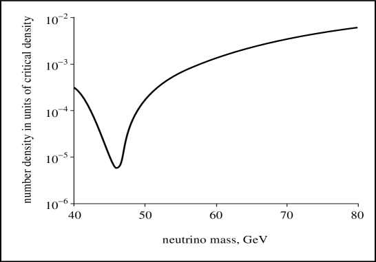
Figure 2: The density of primordial neutrinos in units of the critical density.

After their capture, neutrinos (and antineutrinos) are thermalized, settling in the Earth core, and neutrino-antineutrino pairs start to annihilate. If the equilibrium between capture and annihilation is reached, the annihilation rate is equal to the capture rate. Let us estimate the capture rate ($R_{eq}$) for which the equilibrium between capture and annihilation inside the Earth is reached during the lifetime $t_{E}$ of the Earth. The variation of the number of accumulated neutrinos and antineutrinos $N$ satisfies

$$\frac{dN}{dt}=R_{cap}-R_{ann},$$ (13)

where $R_{cap}$ and $R_{ann}$ denote the capture and annihilation rates respectively. We have

$$R_{ann}=2\int\frac{n^{2}}{4}\left\langle\sigma_{ann}v_{rel}\right\rangle dV.$$ (14)

Here the factor 2 accounts for the fact that in one annihilation a pair of neutrinos disappears; the factor $1/4$ comes from the fact that $n$ denotes the total (neutrinos plus antineutrinos) neutrino density within the thermalized core of the Earth; in $\left\langle\sigma_{ann}v_{rel}\right\rangle$, $v_{rel}$ denotes the relative velocity of thermalized neutrinos. A rough estimate of $R_{ann}$ is obtained by assuming a homogeneous distribution of thermalized neutrinos within a certain volume $V_{therm}$. We define $V_{therm}$ as the volume bounded by the radius which can be reached by a particle of kinetic energy $T_{therm}$ in the center of the Earth freely moving in the Earth potential well. The typical neutrino energy $T_{therm}$ is supposed to correspond to the temperature of the Earth core. The latter is not known exactly, but is around 10000 K. We can therefore consider $T_{therm}=1$ eV as fiducial value. This yields:

$$V_{therm}=\frac{4}{3}\pi R_{therm}^{3},\,\,R_{therm}=\sqrt{\frac{2T_{therm}}{T_{esc0}}\frac{\langle\rho_{E}\rangle}{\rho_{E\,core}}}R_{E},$$ (15)

where $T_{esc0}\equiv\frac{m_{\nu}v_{esc0}^{2}}{2}$, $\langle\rho_{E}\rangle=5.5\,\rm{g/cm^{3}}$ and $\rho_{E\,core}\approx 12\,\rm{g/cm^{3}}$ are the mean and core Earth densities, and $R_{E}$ is the Earth radius. In this approximation we have

$$R_{ann}=\frac{N^{2}}{2V_{therm}}\left\langle\sigma_{ann}v_{rel}\right\rangle\equiv CN^{2}.$$ (16)

It is then easily checked that, neglecting the (slow, linear) variation with time of $R_{cap}$, the solution for the time variation of $N$, or equivalently $R_{ann}$, is $R_{ann}=R_{cap}\tanh^{2}\left(\sqrt{CR_{cap}}\,t\right)$. The “equilibrium” rate $R_{eq}$, for which a balance between capture and annihilation within the Earth lifetime $t_{E}$ is maintained, is therefore estimated to be $R_{eq}=1/(C\,t_{E}^{2})$.

Substituting all the factors, we finally obtain

$$R_{eq}=0.46\times 10^{13}\,{\rm s^{-1}}\,\frac{(4m_{\nu}^{2}-m_{Z}^{2})^{2}+m_{Z}^{2}\Gamma_{Z}^{2}}{m_{\nu}^{7/2}}\left(\frac{T_{therm}}{1\,\rm{eV}}\right)^{3/2}\left(\frac{\langle\rho_{E}\rangle}{\rho_{E\,core}}\right)^{3/2}.$$ (17)

Here the mass of the neutrino, as well as the mass and the width of the $Z$-boson are in GeV. For numerical estimates, we took $\frac{\rho_{E\,core}}{\langle\rho_{E}\rangle}=2$, and (as said above) $T_{therm}=1$ eV.

Having in hands, ready for comparison, the “equilibrium” rate $R_{eq}$, we now come back to the estimate of the capture rate, as given by Eqs.(8)-(11) above. Note that the capture rate of both galactic and slow neutrinos are proportional to the assumed value of the concentration factor $\xi$.

We plot in Fig.3 the total capture rate of neutrinos (summed over slow and galactic ones), as a function of the neutrino mass, for $\xi=2\times 10^{5}$. We also indicate what would be the capture rate if one included only galactic neutrinos.

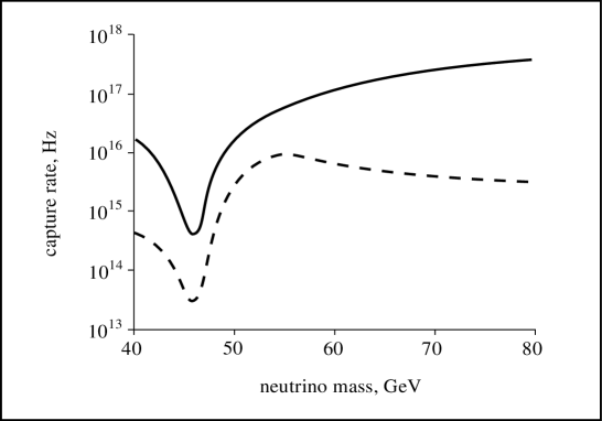
Figure 3: Total capture rate of slow and galactic neutrinos (solid line), compared to the capture rate of galactic neutrinos only (dashed line).

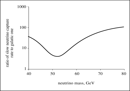
Figure 4: Ratio of the slow neutrino capture rate to galactic one.

The dip at $m_{\nu}\approx 45$ GeV reflects the resonant annihilation dip in primordial neutrino density (see Fig.2). The peak in the galactic neutrino capture rate at $m_{\nu}\approx 55$ GeV comes from the well known fact that when the WIMP mass is equal to the mass of iron nuclei their collision is efficient in slowing down the WIMPs. [This peak is shifted from the iron mass $m_{Fe}=52$ GeV because of the rising relic neutrino density factor.] In the case of the slow WIMPs (which lose their kinetic energy during collisions much more effciently than the fast galactic WIMPs) this “iron resonance” effect is spread over a large range of masses and does not show up as a peak.

In Fig.4 we present the ratio of slow neutrino capture rate to the galactic one. This ratio, obviously, is independent of galactic neutrino density. The dip around $m_{\nu}=m_{Fe}=52$ GeV in Fig.4 is due to the "iron resonance" peak of the galactic neutrino capture.

An important conclusion from Fig.3 is that, in the considered mass range, the equilibrium between capture ($R_{cap}$) and annihilation rates ($R_{ann}$) inside the Earth is established on a time scale smaller than the Earth lifetime. Therefore the annihilation rate can be simply taken as being equal to the (above computed) capture rate: $R_{ann}=R_{cap}$.

To complete the results indicated in Fig.3, we give in Table 2 the galactic and slow neutrino capture rates (in units of $10^{15}\,\rm{s^{-1}}$) for different velocity parameters, and for the special value $m_{\nu}=50$ GeV (and for the standard value $\xi=2\times 10^{5}$). Note that the equilibrium capture rate for $m_{\nu}=50$ GeV amounts to $0.53\times 10^{13}\,\rm{s^{-1}}$.

	$v_{0}=220\,\rm{km/s}$		$v_{0}=266\,\rm{km/s}$
	galactic	slow	galactic	slow
$v_{S}=0$	3.86	18.6	2.88	13.50
$v_{S}=200\,\rm{km/s}$	2.62	12.1	2.14	9.88

Table 2: Capture rates in units of $10^{15}\,\rm{s^{-1}}$ of galactic and slow neutrinos when $m_{\nu}=50$ GeV, for different velocity parameters.

One can see that our results are robust under varying the velocity parameters (retaining the Maxwellian form of the velocity distribution).

In the estimates above, we have not taken into account the effect of the so-called “Sakharov enhancement” of the annihilation rate due to the Coulomb-like attraction mediated by the new $U(1)$ interaction ascribed to neutrinos and antineutrinos of the 4th generation [15]. This interaction has two effects: on one hand it reduces the relic neutrino density (by about 10% if $\alpha_{y}=1/137$, and 25% if $\alpha_{y}=1/50$), but on the other hand it strongly increases the annihilation rate in the Earth. The overall effect is to strongly reduce the equilibration time scale between capture and annihilation in the Earth. Finally, if we were to take into account the "Sakharov enhancement" we would be in the conditions of equilibrium for the whole neutrino mass range considered and for all the acceptable magnitudes of parameter $\xi$.

4 Conclusions

In the present paper we studied the capture by the Earth, and the annihilation in the Earth core, of hypothetical fourth neutrinos (candidate to a sparse sub-dominant component of galactic CDM). We took into account not only the primary “fast” population of neutrinos, but also the recently pointed out secondary “slow” population [10]. It was found that the account of the slow component is crucially important in the considered neutrino mass range, $45<m_{\nu}<90$ GeV. Indeed, the contribution to capture of the slow component is larger by up to the two orders of magnitude than the one of the galactic component (Fig.4).

These results suggest the crucial significance of underground experiments (AMANDA, Super-Kamiokande, Baksan and others) for testing the fourth neutrino hypothesis. For example, Ref. [14] has derived the constraint on WIMP annihilation in the Earth, from AMANDA data, under some assumptions on the annihilation channels, and for a WIMP mass larger than 100 GeV. Making a rough extrapolation of this constraint down to a mass of about 50 GeV one finds a potential sensitivity of the already existing underground neutrino data to the annihilation of a 4th neutrino in the Earth, for almost all the considered interval of neutrino mass. Note, that the presence of the slow component of a 4th neutrino plays a crucial role in this potential sensitivity. Of course, this example can serve only as an illustration, since special analysis of the data in the framework of the hypothesis of a 4th neutrino is needed.

The possibility to distinguish, in underground neutrino experiments, the contribution to annihilation effects of a sparse component of 4th neutrino from the contribution of other WIMPs (presumably dominating in the galactic CDM), results from the combination of several factors. The neutrino capture in the Earth is facilitated by the relatively large weak interaction cross section of a massive neutrino and by the kinematic enhancement of neutrino momentum losses in collisions with iron nuclei. The neutrino annihilation effects in the Earth are strengthened by the relatively large neutrino weak annihilation cross section near $Z$-boson resonance (which is further strongly enhanced by the Coulomb like effect of the new long range interaction), and by the existence of a monochromatic neutrino-antineutrino annihilation channel, specific to a 4th neutrino.

The presence of a slow component qualitatively enhances these factors. The slow component increases by up to 50% the number density of 4th neutrinos near the Earth. Owing to their order-of-magnitude smaller mean velocity, the slow neutrinos are more effectively captured by the Earth (by up to two orders of magnitude) than the galactic ones. In the slow component capture the kinematic peak of iron nuclei capture is spread over the whole considered neutrino mass interval, making it accessible to experimental test. The establishment of kinetic equilibrium between neutrino capture and annihilation in Earth makes the predicted annihilation fluxes insensitive to the details of captured neutrino distribution. As a result, the account of the slow neutrino component makes the hypothesis of a stable massive 4th neutrino accessible to underground neutrino experimental tests even under the most unfavourable astrophysical conditions.

To conclude, our work shows that it is important to analyze existing (and future) underground neutrino data with the view of probing the hypothetical existence of a stable fourth generation neutrino with a mass about 50 GeV. The analysis of the data of MACRO, AMANDA, Kamiokande, Baksan and/or Super-Kamiokande is expected to provide an important probe of (and probably stringent constraints on) this hypothesis, especially in the case where one wishes to explain the DAMA event rate by assuming heavy neutrinos. The existence of a slow 4th neutrino component is crucial in such an analysis because it strongly enhances the underground neutrino flux expected from 4th neutrino annihilation in Earth. This analysis can be viewed as a modest step towards the study of heterotic string phenomenology which generically leads to the prediction of an additional $U(1)$, which, in turn, provides a motivation for considering a stable 4th generation neutrino.

5 Acknowledgement

The work was performed in the framework of the project "Cosmoparticle physics" and was partially supported by the Cosmion-ETHZ and AMS-Epcos collaborations and by a support grant for the Khalatnikov Scientific School.One of us (M.Yu.Kh.) expresses his gratitude to IHES for its kind hospitality and to ICTP for kind hospitality and help in the finishing of this work.

References

- [1] M. Green, J. Schwarz, E. Witten, Superstring theory, Cambridge University Press, 1989.
- [2] D. Fargion, Yu.A. Golubkov, M.Yu. Khlopov, R.V.Konoplich, R. Mignani, Possible effects of the existence of 4th generation neutrino, JETP Letters 69 (N6), 434 (1999); astro-ph/9903086.
- [3] D. Fargion, M.Yu. Khlopov, R.V. Konoplich, R.Mignani, Phys. Rev. D54, 4684 (1996). V.A. Ilyin, M. Maltoni, V.A.Novikov, L.B. Okun, A.N. Rozanov, M.I. Vysotsky, hep-ph/0006324.
- [4] M. Maltoni, M.I. Vysotsky, Phys. Lett. B463, 230 (1999). M. Maltoni, V.A. Novikov, A.N. Rozanov, M.I. Vysotsky, Phys. Lett. B476, 107-115 (2000); hep-ph/9911535.
- [5] S.S. Gershtein, Ya.B. Zeldovich, JETP Lett. 4, 120 (1966). B.W. Lee, S. Weinberg, Phys. Lett. 39, 165 (1977). M.I. Vysotsky, A.D. Dolgov, Ya.B. Zeldovich, Pis’ma v ZhETF 26, 200 (1977). A.D. Dolgov, Ya.B. Zeldovich, Rev. Mod. Phys. 53, 1 (1981).
- [6] Yu.A. Golubkov, R.V. Konoplich, Physics of Atomic Nuclei 61 (N4), 602 (1998); Yad. Fiz. 61 (N4), 675 (1998) (in Russian). D.Fargion, M. Grossi, M.Yu. Khlopov, R.V. Konoplich, astro-ph/9809260.
- [7] K.M. Belotsky, M.Yu. Khlopov, K.I. Shibaev, Monochromatic neutrinos from the annihilation of fourth-generation massive stable neutrino in the Sun and in the Earth, Physics of Atomic Nuclei , 65 (N2), 382 (2002); Yad. Fiz. 65 (N2), 407 (2002) (in Russian).
- [8] L. Krauss, M. Srednicki, F. Wilczek, Phys. Rev., D33, 2079 (1986). T. Gaisser, G. Steigman, S. Tilav, Phys.Rev. D34, 2206 (1986).
- [9] L. Bergström, T. Damour, J. Edsjö, L.M. Krauss and P. Ullio, Implications of a new Solar system population of neutralinos on indirect detection rates, JHEP 9908, 010 (1999).
- [10] T. Damour, L. Krauss, Phys. Rev. Lett. 81, 5726 (1998). T. Damour, L. Krauss, Phys. Rev. D59, 063509 (1999).
- [11] G. Jungman, M. Kamionkowski and K. Griest, Phys. Rep. 267, 195 (1996)
- [12] J.N. Bahcall and M.N. Pinsonneault, Rev. Mod. Phys. 64, 885 (1992)
- [13] A. Gould, Astrophys. J. 321, 571 (1987).
- [14] AMANDA collaboration, astro-ph/0012285.
- [15] K.M. Belotsky, M.Yu. Khlopov, K.I. Shibaev, Sakharov’s enhancement in the effect of 4th generation neutrino, Grav.&Cosm. 6, 140, Supplement, (2000).