BL Lacertae: complex spectral variability and rapid synchrotron flare detected with $Beppo$SAX

We report on two BeppoSAX observations of BL  Lac (2200+420) performed respectively in June and December 1999, as part of a ToO program to monitor blazars in high states of activity. During both runs the source has been detected up to 100 keV, but it showed quite different spectra: in June it was concave with a very hard component above 5-6 keV ($\alpha_{1}\sim 1.6$; $\alpha_{2}\sim 0.15$); in December it was well fitted by a single power law ($\alpha\sim 0.6$). During the first BeppoSAX observation BL  Lac showed an astonishing variability episode: the $0.3-2$ keV flux doubled in $\sim 20$ minutes, while the flux above 4 keV was almost contant. This frequency–dependent event is one of the shortest ever recordered for BL Lac objects and places lower limits on the dimension and magnetic field of the emitting region and on the energy of the synchrotron radiating electrons. A similar but less extreme behaviour is detected also in optical light curves, that display non-simultaneous, smaller fluctuations of $\sim 20\%$ in 20 min. We fit the spectral energy distributions with a homogeneous, one-zone model to constrain the emission region in a very simple but effective SSC + external Compton scenario, highlighting the importance of the location of the emitting region with respect to the Broad Line Region and the relative spectral shape dependence. We compare our data with historical radio to $\gamma$-ray Spectral Energy Distributions.

1 Introduction

Blazar objects are highly variable sources characterised by non–thermal emission that dominates from the radio to the $\gamma$-rays. This emission is supposedly due to a relativistic jet seen at a small angle to the line of sight (Blandford & Rees 1978). Although blazars emit over the entire electromagnetic spectrum, their variability seems to be more pronounced in the optical-X-ray band than the radio-infrared one, both in term of flux and time scale (Ulrich et al. 1997). It is also well known that the overall spectral energy distribution (SED) of blazars shows (in a $\nu$ vs $\nu F_{\nu}$ representation) two broad emission peaks; a lower frequency peak believed to be produced by synchrotron emission and a higher frequency peak probably due to the inverse Compton process. However, during strong variability events, the overall SED can change significantly. For instance, changes up to few orders of magnitude in the position of the synchrotron peak have been detected during flares in Mkn 501 (Pian et al. 1998) and 1ES 2344+514 (Giommi et al. 2000). Incidentally, both sources belong to the HBL class, High Frequency Peaked blazars, with the synchrotron peak in the UV – X-ray band. A key to understand blazar variability is the acquisition of wide band spectra during major flaring episodes. Spectral and temporal information greatly constrain the jet physics, since different models predict different variability as a function of wavelength.

To this end, we started a project to observe with the BeppoSAX satellite (Boella et al. 1997a) blazars while they were in an active state as detected in the optical, X-ray or TeV bands. As part of this program, we already observed the two sources ON 231 and PKS 2005-489 (Tagliaferri et al. 2000, 2001). Here we present two BeppoSAX observations of the third observed source, BL Lac itself, carried out in June and December 1999, together with simultaneous optical and radio data. Other two observations have been carried out on the objects OQ 530 and S5 0716+714 (paper in preparation).

BL Lacertae, being the prototype of the BL  Lac class, is one of the best–studied objects. It is a featureless LBL (low frequency peaked blazars) object, but sporadically it shows optical emission lines (EW $\sim 6$ Å; Vermeulen et al. 1995; Corbett et al. 2000). In the X-ray it has been observed by many satellites; Einstein detected a photon index of $1.68\pm 0.18$ (Bregman et al. 1990), Ginga a photon index in the range 1.7-2.2 (Kawai et al. 1991); ROSAT a photon index of $1.95\pm 0.45$ (Urry et al. 1996). ASCA observed BL Lac in 1995 detecting a photon index of $1.94\pm 0.04$ (Madejski et al. 1999; Sambruna et al. 1999). In July 1997 following an optical outburst, it was observed with EGRET, RossiXTE and ASCA. EGRET found that the flux level above 100 MeV was 3.5 times higher than that observed in 1995 (Bloom et al. 1997). RossiXTE found a harder spectrum with a photon index in the range 1.4-1.6 over a time span of 7 days (Madejski et al. 1999). A fit to simultaneous ASCA and RossiXTE data shows the existence of a very steep and varying soft component below 1 keV, photon index in the range 3-5, in addition to the hard power law component with a photon index of 1.2-1.4. Two rapid flares with time scales of 2-3 hours were detected by ASCA but only in the soft part of the spectrum (Tanihata et al. 2000). Finally, in November 1997, BL Lac was observed with BeppoSAX that detected a photon index of $1.89\pm 0.12$ (Padovani et al. 2001).

The BeppoSAX observations presented here were triggered when the source was in very high optical states (R $\sim 12.5$), but when the source was actually observed by BeppoSAX the optical flux was lower (R = 13.4 - 13.6). In both observations the source was clearly detected up to 100 keV giving us the possibility to study BL Lac over an unprecedentedly large spectral range (0.3-100 keV) with simultaneous data.

2 X-ray observations

2.1 Observations and Data Reduction

The BeppoSAX satellite carries on board four Narrow Field Instruments (NFI) pointing in the same direction and covering a very large energy range from 0.1 to 300 keV (Boella et al. 1997a). Two of the four instruments have imaging capability, the Low Energy Concentrator Spectrometer (LECS), sensitive in the range 0.1–10 keV (Parmar et al. 1997), and the three Medium Energy Concentrator Spectrometers (MECS) sensitive in the range 1.3–10 keV (Boella et al. 1997b). Only two MECS detectors were functioning at the time of our observation. The LECS and MECS detectors are all Gas Scintillation Proportional Counters and are at the focus of identical grazing incidence X–ray telescopes. The other two are passively collimated instruments: the High Pressure Proportional Counter (HPGSPC), sensitive in the range 4–120 keV (Manzo et al. 1997) and the Phoswich Detector Systems (PDS), sensitive in the range 13–300 keV (Frontera et al. 1997). For a full description of the BeppoSAX mission see Boella et al. (1997a).

date	LECS	count ratea	MECS	count rateb	PDS	count ratec
	exposure (s)	$\times 10^{-2}$ cts  s-1	exposure (s)	$\times 10^{-2}$ cts  s-1	exposure (s)	cts  s-1
5-7 June 1999	45253	$7.14\pm 0.14$	54404	$11.1\pm 0.2$	$3.9\times 10^{4}$	$0.16\pm 0.02$
5-6 December 1999	17543	$8.81\pm 0.25$	54677	$17.8\pm 0.19$	$2.4\times 10^{4}$	$0.18\pm 0.03$
	B	V	Rc	Ic	$\alpha_{opt}$ d
			magnitudes
06 June 1999	$15.01\pm 0.03$	$14.13\pm 0.03$	$13.52\pm 0.03$	$12.79\pm 0.03$	$1.35\pm 0.06$
06 December 1999	$15.33\pm 0.03$	$14.26\pm 0.03$	$13.49\pm 0.03$	$12.69\pm 0.03$	$2.02\pm 0.06$

Table 1: Journal of observations. ^a In the band 0.1–10 keV; ^b for two MECS units in the band 1.5–10 keV; ^c in the band 12–100 keV; ^d calculated from mJy fluxes. Optical data were dereddened using A${}_{V}=1.09$.

The log of the BL Lac observations is given in Table 1, together with the exposure times and the mean count rates in the various instruments. The data analysis for the LECS and MECS instruments was based on the linearized, cleaned event files obtained from the online archive (Giommi & Fiore 1998). Light curves and spectra were accumulated with the FTOOLS package (v. 4.0), using an extraction region of 8 and 4 arcmin radius for the LECS and MECS, respectively. The LECS and MECS background is low and rather stable, but not uniformly distributed across the detectors. For this reason, it is better to evaluate the background from blank fields, rather than in concentric rings around the source region. Thus, after having checked that the background was not varying during the whole observation by analyzing a light curve extracted from a source–free region, we used for the spectral analysis the background files accumulated from long blank field exposures and available from the SDC public ftp site (see Fiore et al. 1999, Parmar et al. 1999).

The PDS was operated in the customary collimator rocking mode, where half the collimator points at the source and half at the background and they are switched every 96 s. The data were analysed using the XAS software (Chiappetti & Dal Fiume 1997) and the data reduction was performed according to the procedure described in Chiappetti et al. (1999), inclusive of spike filtering.

The source was not detected by the HPGSPC detector.

2.2 Spectral analysis

The spectral analysis was performed with the XSPEC 10.0 package, fitting together the LECS, MECS and PDS data. To fit the data of these detectors simultaneously, one has to allow for a constant rescaling factor to account for intercalibration systematics of the instruments. The acceptable values for these constants are in the range 0.67-1 for the LECS and in the range 0.77-0.93 for the PDS, with respect to the MECS (Fiore et al. 1999). In order to reduce the number of fitting parameters, during the parameter error search we fixed the two constants at the best-fit values of 0.72 and 0.9 in all our fits, respectively. The LECS data have been considered only in the 0.1–4 keV interval, as suggested by SDC team (Fiore et al., 1999). We first considered the June observation. We fitted the data with a single power law plus free interstellar absorption. The 0.3-100 keV X-ray spectrum of June is not well fitted by this model, showing large residuals above 10 keV (see fig. 1 bottom panel and Table 2) and best fit estimate of N_H significantly lower than the Galactic interstellar value of N${}_{\rm H}=2.02\pm 0.01\times 10^{21}$ cm^-2 (Elvis et al. 1989). A good fit to the data is obtained using a sum of two power laws (see fig. 1 top panel and Table 2). The energy intersection falls between 5 and 6 keV. Below we detect a softer component ($\alpha=1.6\pm 0.25$), probably due to synchrotron emission, while above we observe a harder component ($\alpha=0.15\pm 0.22$), supposedly originating from inverse Compton emission. The interstellar absorption is higher than the Galactic one and is consistent with previous results (Sambruna et al., 1999; Madejski et al., 1999). This X-ray spectrum is very similar to the one observed for ON 231, while it was in an active state (Tagliaferri et al. 2000). A break in the combined ASCA and RossiXTE 0.7-20 keV spectrum was also detected during a short flaring state of BL Lac in July 1997 (the RossiXTE exposure time was of about 30 minutes). However, besides the source being in a higher state, the break was at about 1 keV and the synchrotron spectrum was much steeper, with an energy index $\alpha=2.7$ (Tanihata et al. 2000). Thus, although in both cases the synchrotron and the Compton components were simultaneously detected, the X-ray spectrum of BL Lac was quite different. During the July 1997 outburst the Compton component was brighter, while during our June 1999 observation the synchrotron component increased its contribution to the overall X-ray spectrum, dominating up to $\sim 5$ keV.

Figure 1: Top panel: LECS+MECS+PDS BL Lac spectrum during the June 1999 observation, the best fit model is a sum of two power laws. Bottom panel: the same spectrum fitted with a power law model (over the entire energy range), clearly showing that a simple power law model can not fit the data.

After the June 1999 BeppoSAX observation, the source remained active in the optical, with the R magnitude ranging between $\sim 12.6-13.8$ mag. At the end of November it brightened again to R$\sim 12.4$, thus we triggered a second BeppoSAX ToO observation. However, when the source was observed in the X-rays the R magnitude was down to R$\sim 13.5$. During this second observation, the X-ray spectrum was in a quite different state. In this case the 0.3-100 keV spectrum is well fitted by a single power law model (see Table 2). The total flux in the 2-10 keV energy band is about a factor of two higher than in June. However, the two spectra cross at about 1.5 keV, thus the flux in the softer X-ray energy band is actually lower. Clearly, the overall shape of the SED changed between the two observations and during the second one we detected mostly the Compton component. The 2-10 keV flux is very similar to the value detected during the June 1997 BeppoSAX observation, which was also well fitted by a single power law that is a little bit steeper, $\alpha=0.89\pm 0.12$, (Padovani et al. 1998, 2001).

Date	NH	$\alpha_{1}$	$\alpha_{2}$	$F_{1keV}$	$F_{0.5-2keV}$	$F_{2-10keV}$	$F_{10-100keV}$	$\chi_{r}^{2}/d.o.f.$
	$\times 10^{21}\ {\rm cm^{-2}}$			$\mu$Jy	ergs cm-2 s-1	ergs cm-2 s-1	erg cm-2 s-1
5-7 June	$1.41\pm 0.02$	$1.04\pm 0.03$		1.77	$0.4\times 10^{-11}$	$0.6\times 10^{-11}$	$0.86\times 10^{-11}$	$1.2/124$
5-7 June1	$2.42\pm 0.04$	$1.57\pm 0.25$	$0.15\pm 0.22$	$0.77$	$0.4\times 10^{-11}$	$0.6\times 10^{-11}$	$2.48\times 10^{-11}$	$1.03/122$
5-6 Dec.	$2.49\pm 0.05$	$0.63\pm 0.06$		$0.96$	$0.35\times 10^{-11}$	$1.2\times 10^{-11}$	$3.67\times 10^{-11}$	$1.02/130$

Table 2: ¹The two power laws cross at $\sim 5.5$ keV.

The interstellar absorption, $N_{\rm H}$, plays an important role in fitting the X-ray spectrum of BL Lac, due to its high value and to the presence of a molecular cloud in the line of sight (Lucas & Liszt, 1993). To determine the best $N_{\rm H}$ value to use to fit the X-ray spectrum of BL Lac, we repeated the fitting process fixing the $N_{\rm H}$ both to the Galactic column density of neutral hydrogen from 21 cm measurements $N_{\rm H}=2\times 10^{21}$ cm^-2 (Elvis et al., 1989) and to the higher value $N_{H}=3.6\times 10^{21}$ cm^-2 obtained taking also to consideration the absorption due to the presence of the molecular cloud. In the first case, we cannot find a good fit to the data for both observations. The second value gave an acceptable fit for the first observation ($\chi_{r}^{2}/d.o.f.=1.06/123$): an F-test suggested that letting $N_{H}$ remain free does not produce a significant improvement in the quality of the fit. This is not true for the December spectrum: for this observation, letting $N_{H}$ remain free gives a probability $\geq 95\%$ of improving the quality of the fit. Thus, we kept the $N_{H}$ free to vary in both observations, finding values that are perfectly consistent. A similar value was also found by Padovani et al. (2001) for the first BeppoSAX observation. Given that the LECS is well suited for the determination of the interstellar absorption in the X-ray band, we think that the value found in three different BeppoSAX observations (and with different best fit models) should be the one used for the analysis of the BL Lac X-ray data. Thus, the value used for the analysis of the ASCA data is probably too high (Sambruna et al. 1999, Tanihata et al. 2000).

Figure 2: In the December 1999 observation the data are well fitted by a single power law model plus an interstellar absorption value perfectly consistent with the value obtained for June’s spectrum.

2.3 Temporal analysis

The X-ray light curve of the June observation looks in general quite constant. However, it reveals an amazing feature about 42 hours after the beginning of the measurements. In a very short timescale, about 20 minutes, the [0.3-2 keV] flux doubled: this is the fastest variability ever measured for BL Lac. In 2 hours the soft X flux increased 4 times and then decreased to former values. This is not frequency–independent: as can be seen in Fig. 3, variations are detected only in the softer spectral component. While the synchrotron emission is extremely variable, the inverse Compton component remains almost constant during the observation. This behaviour is very similar to that observed for S5 0716+714 (Giommi et al. 1999) and ON 231 during a high state (Tagliaferri et al. 2000). Also in these cases fast variability was detected only for the synchrotron part of the spectrum . A similar behaviour for BL Lac has been observed with ASCA during the July 1997 campaign, when the source was in a high state. Again, rapid variability was detected only in the soft part of the X-ray spectrum, with the 0.7-1.5 keV flux flaring a couple of times by a factor of two on time scales of 3-4 hours, while above 3 keV no rapid variability was found (Tanihata et al. 2000). In analogy with the BeppoSAX observations of ON 231 and BL Lac one would expect that also in the ASCA data there is a break between 1-3 keV, reflecting the presence of the synchrotron tail responsible for the fast variability below 1.5 keV and of the less variable Compton component above 3 keV. However, the presence of this break is not so clear in the ASCA data and only in a simultaneous RossiXTE and ASCA spectrum can one see that the spectrum is much steeper below 1 keV (Tanihata et al. 2000). Once again, the BeppoSAX large spectral energy range combined with its good sensitivity and energy resolution is unique in determining the X-ray spectral shape of bright blazars in the range 0.1-100 keV.

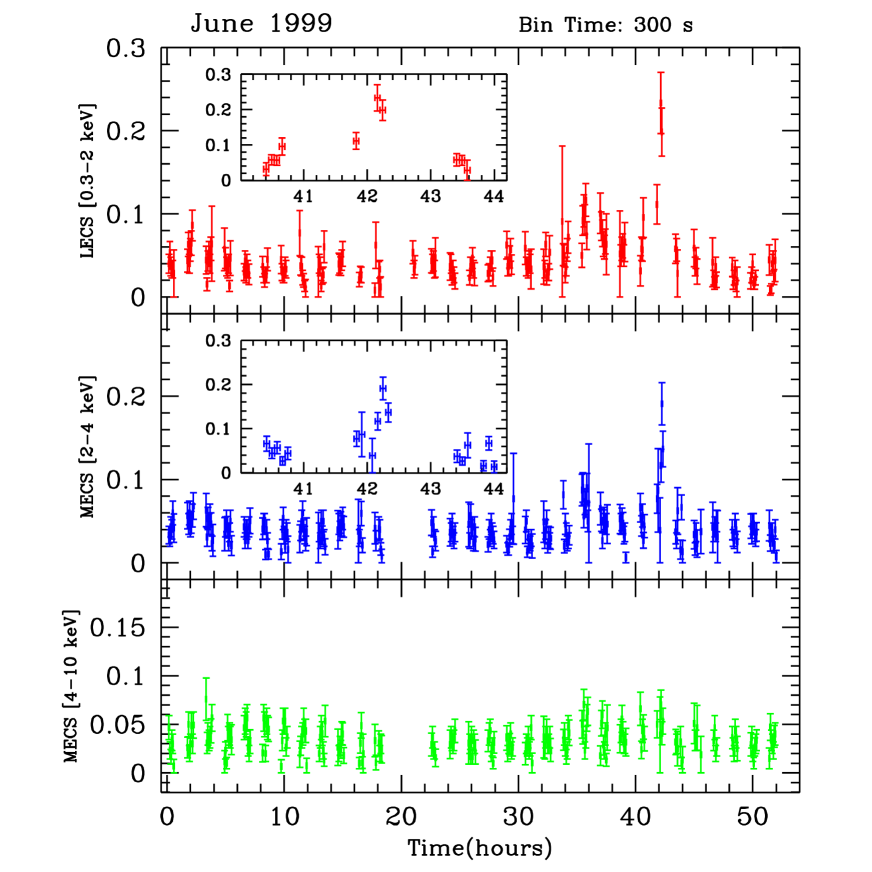
Figure 3: LECS 0.3-2 keV (top panel), MECS 2-4 keV (mid panel) and MECS 4-10 keV (bottom panel) light curves of BL Lac during the June 1999 BeppoSAX observation. Note the clear flare detected at the end of the observations by different detectors (top and mid panels) and better shown in the insert. Note also that above the spectral break, i.e. in the Compton component, the flare is clearly not present (bottom panel).

The light curves of the December observation do not reveal variability, but this is not surprising as BeppoSAX detected only the inverse Compton component.

3 Optical observations

During the BeppoSAX observations BL Lac was intensively monitored in the optical by several observers (see Table 3) located at different longitudes around the world, belonging to the Whole Earth Blazar Telescope (WEBT) collaboration (Villata et al. 2000). This collaboration, begun in 1997, aims to provide 24 hour coverage of Blazars.

Group	Bands	Tel.	detector
Abastumani	B,V,R,I	70 cm	Texas TC241
Lowell Obs.	V, I	180 cm	SITe 501A
Foggy Bottom	R,I,V	40 cm	CCD
Kyoto	R	25 cm	Kodak KAF 400
Perugia	R, I	40 cm	Texas TC211
Roma I	V	50 cm	Texas TC241
Roma II	I	35 cm	SITe 501A
Torino	B,V,R,I	105 cm	Astromed EEV CCD

Table 3: WEBT optical telescopes participating in the BL Lac campaign. Roma I is located in Vallinfreda, Roma II in Greve

Each group performed differential photometry of BL Lac with respect to 4 nearby reference stars (Bertaud et al. 1969; Fiorucci & Tosti 1996). The data were then checked for systematic effects and finally a self-consistent light curve of BL Lac was obtained.

Not all the involved observers used the same filters (see Table 3), nor made observations with all the filters. To build an optical light curve as complete as possible in time coverage we transformed observations in different bands into the I band, using appropriate colour indices for each Observatory. A small change of the colour index with the source luminosity (0.06 in V-I for a change of 0.2 R mag) was clearly detected in the Abastumani data set, but it does not seriously affect the transformation of the observed magnitudes from other bands into the I band, so that the long-term behaviour of the source during the run can be safely traced. The resulting light curve for the June pointing is plotted in Fig. 4 (lower panel) together with the X-ray one (upper panel) for comparison.

It is apparent from Fig. 4 that BL Lac varied continuously during the BeppoSAX pointing with an overall amplitude of 0.55 mag. After the maximum at I=12.45 just before the beginning of the BeppoSAX observation, followed by a decay of about 0.4 mag in less than 10 hours, the source behaviour was characterised by an increasing trend for about one day, with small oscillations; the brightness then decreased, with a short plateau, down to I = 13.

The comparison with the X-ray light curve is not easy, due to the different time sampling and accuracy of the two curves. In any case the amplitude of the X-ray variability is much wider than the optical one. The most striking feature of the X-ray light curve, i.e. the strong and fast flare discussed above, has no optical counterpart, while a temporal coincidence may be found between the smaller X-ray flare at JD 1336.3 and the fast decrease in the optical. However this cannot be stated for sure, due to the X-ray error bars and the lack of continuity in the optical light curve. It is interesting to note that this optical event occurred about 6 hours before the stronger soft X-ray flare, that does not seem to have an optical counterpart. Thus, it seems that there is not a one–to–one connection between fast X-ray and optical variability.

During the second run (December) the weather was not so good and the coverage from the ground was less complete. The average flux level in the I band was 12.6, about the same as in June, while the (V-I) colour index was substantially steeper ($\sim 1.6$). The source showed a monotonic decrease of 0.2 mag at the beginning of the observing run and then remained nearly constant. Linear polarization was measured on December 14, 1999, at a level of $4\%$ (Tommasi et al., 2001).

Simultaneous values of magnitudes for the June and December pointing are given in Table 1, together with the derived spectral slopes. The steep spectral slope, when extrapolated to the soft X-rays, predicts a flux below the observed one, confirming the interpretation of the observed X-ray spectrum as due to the Inverse Compton component. This behaviour is in agreement with the X-ray light curve, which remained constant during the second pointing.

Figure 4: Soft X-ray and optical (I band) light curves of BL Lac during 1999 June, 5-7. The scale of variability is also reported in the two panels.

4 Discussion

During our two BeppoSAX observations, BL Lac showed two different spectral shapes not only in the X ray band, but also in the optical one. Even if optical fluxes are almost similar, the spectrum in June is harder than in December. Optical magnitudes, fluxes and spectral indices are listed in Table 1. The synchrotron spectrum of December seems to be shifted toward lower energies than that of June: its optical spectrum is softer and BeppoSAX detected just the inverse Compton component. The observed Compton spectra are quite different, as we already mentioned, being much harder in June ($\alpha_{C}=0.15$) than in December ($\alpha_{C}=0.63$), and even more so with respect to the previous BeppoSAX observation ($\alpha_{C}=0.9$, Padovani et al. 2001). In a simple picture one would have expected that the presence of a break in the X-ray spectrum, and hence of a synchrotron component, would have implied a higher source flux. But this is not the case. Although the flux below 1.5 keV was higher during the observation with the spectral break, the 2-10 keV flux was higher in the other two BeppoSAX observations. All this can be explained by the fact that both the synchrotron, as shown by the high optical state, and the Compton components are varying. In June, the synchrotron flux prevails in the soft X-ray band and two components are detected in the X-ray spectrum. However, the 2-10 keV band is still dominated by the Compton emission, which is lower but unusually hard.

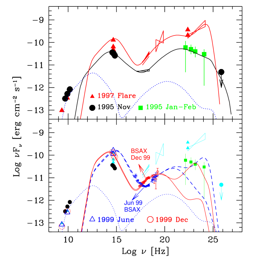
Figure 5: Four simultaneous SEDs of BL Lac together with our best fit models. For the 1995 SED see Sambruna et al. (1999), for the 1997 SED see Madejski et al. (1999). For the two BeppoSAX observations the simultaneous radio data are from NRAO, while the optical data are from our observations. Note that the EGRET data of 1995 are not simultaneous with the other data of the same year. Top panel: the 1997 data modeled with a synchrotron inverse Compton model where the emission line photons are important for the formation of the very high energy spectrum. Note however that the emission in the entire X–ray band is produced by the synchrotron self–Compton process. For the 1995 SED, the fainter and steeper EGRET spectrum suggests that the emission line photons are not important. Consequently we have assumed that the emitting region is located beyond the BLR. Bottom panel: triangles and circles correspond to the SEDs of June and December 1999, as labeled. For comparison we also report the 1995 and 1997 SEDs (crosses). For each SEDs, we show the models corresponding to important or negligible emission line radiation for the formation of the $\gamma$–ray spectrum. For comparison, we also plot the 1995 and 1997 data in light grey. In both panels we also show the calculated emission produced in a much larger region of the jet, to account for the radio flux (dotted line).

To show the complex behaviour of the spectral emission of BL Lac we plot in Fig. 5 four different SEDs corresponding to the multi-wavelength campaigns carried out during November 1995, during July 1997, when the source was in a very high state and during our two BeppoSAX observations. This figure clearly shows the high degree of variability and complexity of BL Lac’s SED.

4.1 Limits on magnetic field and particle energies

During the BeppoSAX observation of June 1999, the X–ray flux below 4 keV varied by a factor 2 in 20 minutes (see Fig. 3). This is one of the fastest variability episodes ever observed at any frequency in a BL  Lac object, to be compared with a very similar timescale observed in the TeV band in Mkn 421 (Gaidos et al. 1996; see also Maraschi et al. 1999 and Fossati et al. 2000 for the correlation between the X–ray and TeV emission). Interestingly, the higher energy X–rays, belonging to the flat part of the observed spectrum, did not vary. This suggests that, in the two X–ray bands, we see the emission by a different part of the electron population: the highest energy electrons, that form the steep tail of the synchrotron spectrum, radiatively cool more rapidly than electrons producing the inverse Compton part of the spectrum visible above $\sim 5$ keV. This implies that a similarly fast variability should be observed in the tail of the Compton spectrum (as indeed was the case for Mkn 421).

The size of the region emitting the variable X–rays must be $R<ct_{var}\delta$, where $\delta\equiv[\Gamma(1-\beta\cos\theta)]^{-1}$ is the beaming factor. $\Gamma$ and $\beta$c are the bulk Lorentz factor and the bulk velocity, respectively, and $\theta$ is the viewing angle.

We then require that the cooling time (in the comoving frame) is shorter than $R/c$ for those electron emitting at $\nu=10^{17}\nu_{17}$ Hz. This in turn implies a lower limit on the magnetic field and an upper limit on the energy of the electrons emitting at $\nu$:

$$B\,>\,1.2\,t_{h}^{-2/3}(1+U_{B}/U_{r})^{-2/3}\nu_{17}^{-1/3}\delta^{-1/3}(1+z)^{1/3}\,\,{\rm G}$$ (1)

$$\gamma\,<\,1.5\times 10^{5}\,t_{h}^{1/3}(1+U_{B}/U_{r})^{1/3}\nu_{17}^{2/3}\delta^{-1/3}(1+z)^{1/3}$$ (2)

where $t_{h}$ is the variability timescale in hours and $U_{B}/U_{r}$ is the magnetic to radiation energy density ratio (we implicitly assume that Klein Nishina effects are negligible). Using $t_{h}=1/3$, $U_{B}/U_{r}=1$ and $\nu_{17}=1$ we derive $B>1.6\delta^{-1/3}$ G and $\gamma<1.3\times 10^{5}\delta^{-1/3}$.

More severe limits can be set by the optical variations, in the $I$ band ($\nu\sim 4\times 10^{14}$ Hz) of about 20 per cent in 20 minutes. Assuming a doubling time of 1.5 hours, we obtain $B>3.7\delta^{-1/3}$ G and $\gamma<5.5\times 10^{3}\delta^{-1/3}$.

Above 4 keV, the radiation is due to the inverse Compton process, and are characterized by smaller energies than those producing the synchrotron tail. Their random Lorentz factor can be estimated assuming that the relevant seed photons have frequencies $\sim 10^{14}$ Hz (i.e. the synchrotron peak), resulting in $\gamma\sim 100$. Assuming $B>3.7\delta^{-1/3}$ G, their cooling time (in our observing frame) is less than $\sim 78\delta^{-1/3}$ hours, which comfortably allows for the non–detection of variability in the hard X–ray band. Longer timescale are derived in the case of scattering with photons of the BLR, since in this case the relevant electron energies producing photon in the hard X–ray band are smaller.

4.2 Homogeneous synchrotron inverse Compton models

We have applied a homogeneous, one–zone synchrotron inverse Compton model to the four SEDs shown in Fig. 5 (Ghisellini et al. 199). The model assumes that the source is spherical, of radius $R$, magnetic field $B$ and it moves with a bulk Lorentz factor $\Gamma$. Radiation is beamed with the Doppler factor $\delta$. Throughout the source we inject relativistic particles continuously, at the rate $Q(\gamma)\propto\gamma^{-s}$ cm^-3 between $\gamma_{min}$ and $\gamma_{max}$. We derive the stationary particle distribution solving the continuity equation, taking into account radiative cooling, electron-positron pair production, and approximating the Klein–Nishina cross section, for the scattering process, by a step function, equal to the Thomson cross section if the seed photon has energy $h\nu\leq m_{e}c^{2}/\gamma$ and zero otherwise.

In the absence of pair production and if the Klein–Nishina effects are negligible, the particle distribution is a broken power law: $N(\gamma)\propto\gamma^{-2}$ below $\gamma_{min}$ and $N(\gamma)\propto\gamma^{-(s+1)}$ above.

The seed soft photon distribution is provided by the synchroton process only if the source is located at a distance, along the jet, greater than a critical distance $z_{BLR}$ where most of the line emission is produced. Otherwise, we include the radiation energy density of the emission lines, as seen in the frame comoving with the source.

The applied model is aimed at reproducing the spectrum originating in a limited part of the jet, thought to be responsible of most of the emission. This region is necessarily compact, since it must account for the fast variability. Therefore the radio emission from this compact regions is strongly self–absorbed, and the model cannot account for the observed radio flux. We have then calculated the spectrum produced in a much larger region of the jet (with dimension $R=7\times 10^{17}$ cm), to account for the radio flux. This spectrum is shown in Fig. 5 with the dotted line, and the input parameters are listed in Table 4.

The observed variability timescale $t_{var}\sim 20$ minutes severely limits the dimension of the compact source to be $R<ct_{var}\delta\sim 3.6\times 10^{13}\delta$ cm. We have assumed $\delta=20$ and $R=7\times 10^{14}$ cm for the SEDs of the 1997 flare and for the two SEDs observed by us in 1999. For the 1995 data, instead, we have assumed a dimension 10 times larger.

This choice is suggested by comparing the overall SEDs of 1995 and 1997: as can be noted, there is a large difference in the emission at high energies above 100 MeV, which has been interpreted (Sambruna et al. 1999; Böttcher & Bloom 2000, Madejski et al. 1999) as a different contribution of the external seed photons for the formation of the Compton spectrum. In 1995, the steep and relatively weak $\gamma$–ray emission favours SSC as the main emission process, while the flat and strong $\gamma$–ray emission during the 1997 flare suggests that external seed photons are relevant.

BL Lac has indeed shown variations in the intensity of the emission lines, which have sometimes exceeded the canonical threshold of 5 Å of equivalent width to define an objects as belonging to the BL  Lac class (Vermeulen et al. 1995). However, the observed variation are within a factor of 3 in absolute intensity, and it is not clear if this is enough to influence strongly the production of the high energy emission.

Date	In/Out	$L^{\prime}$	$R$	$B$	$U^{\prime}_{ext}$	$\delta$	$s$	$\gamma_{min}$	$\gamma_{max}$
		erg s-1	cm	G	erg cm-3
1995	Out	9.0e40	7e15	0.2	…	20	2.8	3.5e3	5.0e5
1997	In	5.2e41	7e14	4.0	1	20	3.8	1.5e3	3.0e4
1999 Jun	Out	1.3e41	7e14	1.2	…	20	3.7	1.1e3	1.0e5
1999 Jun	In	1.6e41	7e14	1.1	1	20	3.7	1.2e3	5.0e4
1999 Dec	Out	1.0e41	7e14	13	…	20	3.7	4.7e2	1.0e4
1999 Dec	In	1.1e41	7e14	13	1	20	3.8	4.7e2	1.0e4
Large	Out	5.2e39	7e17	1.2e-3	…	20	2.8	6.0e3	1.0e5

Table 4: Input parameters for the SSC models

We propose here an alternative scenario, based on the idea that the dissipation region of the jet corresponds to the collision of two blobs or shells moving at slightly different velocities (the “internal shock” scenario for blazars, see Ghisellini 1999; Spada et al. 2001, Madejski et al. 1999). If the bulk Lorentz factor of the two shells differs by a factor 2, a later but faster shell catches up with an earlier and slower one at a distance $z\sim\Gamma^{2}z_{0}$, where $z_{0}$ is the initial separation and $\Gamma$ is the Lorentz factor of the slower shell. We therefore have that different SEDs correspond to different collisions, that can occur at different location in the jet. Some of them may be located within the size of the BLR, while others occur outside. This has a quite dramatic effect on the spectrum, since within the BLR the energy density of the emission line radiation (as measured in the comoving frame) easily exceeds the magnetic and the synchrotron energy densities. Therefore, collisions occurring at $z<z_{BLR}$ emit most of their power in the GeV band, as happened in the 1997 flare. On the contrary, for collisions beyond $z_{BLR}$ the emission line radiation is negligible, and the Compton to synchrotron luminosity ratio is controlled by the ratio between the magnetic field and the synchrotron energy densities.

We can estimate the size of the BLR of BL Lac by adopting the correlation presented by Kaspi et al. (2000) between the ionizing luminosity and the size of the BLR. We derive $z_{BLR}\sim$3–5$\times 10^{16}$ cm.

For the two SEDs observed by us in 1999, we unfortunately lack the high energy EGRET data, which best discriminate between collisions occurring inside/outside the BLR. In fact, the medium–hard energy X–rays are always produced by the SSC process, even in the flare of the summer 1997, and therefore the X–ray flux level and spectrum do not reflect the importance of the external seed photons.

For the 1999 June SED, the very short variability timescale suggests a very compact region, and hence a location, along the jet, close to the jet apex (a transverse dimension $R=7\times 10^{14}$ cm translates into a radial distance $z\sim R/\sin\psi=7\times 10^{15}$ cm for a jet semi–opening angle $\psi=0.1$). For these data we therefore prefer an inverse Compton region within the Broad Line Region (“IN” in table 4) choice. For the 1999 December observation we do not have tight constraints from variability, and one should consider both regions within and outside the BLR.

In any case, for both the June and December 1999 SEDs, we show the calculated spectra for both options, to illustrate the difference in the predicted high energy spectra.

In Table 4 we list the relevant input parameters of the model. As can be seen the different SEDs can be explained by using the same intrinsic luminosity, apart from the 1997 flare case (which has 5 times more power than the other SEDs). What largely differs among the different cases is the value of the magnetic field and the value of $\gamma_{min}$, which controls the location of both the synchrotron and the Compton peaks and their relative amplitude.

5 Conclusions

BeppoSAX observations of BL  Lac in 1999 reveal the extremely complex behaviour of this source, as confirmed by the comparison with previous multiwavelength observations. During the June observation, soft X-ray light curves were characterized by the fastest variability episode ever recordered for BL  Lac: the flux below 4 keV doubled in 20 minutes while remaining constant at higher energies. Such an amazing event allows us to put severe constraints on the dimension of the X-ray emission region, on the magnetic field and on the emitting particle energies. The frequency dependence is easily explained when performing the spectral analysis, that highlights a spectral break attributed to the transition from the more variable synchrotron to a very hard inverse Compton spectrum: synchrotron X-ray emitting electrons are more energetic than Compton ones, so they cool faster. During the second 1999 run, BeppoSAX detected a softer Compton component along its whole spectral range, which accounts for the constance of the light curves. The comparison of 1995 and 1997 BL  Lac Spectral Energy Distributions, extending to $\gamma$-ray energies, suggests the implication of different inverse Compton emission models. Furthermore, the constance of external radiation, as inferred from the constance of emission lines, implies that the emitting shell should be differently located with respect to the Broad Line Region, in order to explain the different observed high energy spectra. Unfortunately our observations lack simultaneous $\gamma$-ray data, which are essential to discriminate between various high energy emission models. Therefore, we have calculated the Spectral Energy Distribution resulting from different possible locations of the emitting shell, adopting an internal shock model. Taking into consideration the hints given by variability and X-ray spectral shape, the most viable scenario to explain our multiwavelength BL  Lac observation of 1999 June implies that the emitting shell is internal to the Broad Line Region, thus producing $\gamma$-ray emission via Compton scattering with external photons. The 1999 December data are less revealing and we cannot discriminate between the two possible locations.

- (1) Bertaud C., Dumortier B., Veron P., Wlerick G., Adam G., Bigay J., Garnier R., Duruy M., 1969, A&A 3, 436
- (2) Blandford R.D., Rees M.J., 1978, in: Pittsburgh Conference on BL Lac Objects, Pittsburgh, University of Pittsburgh, 1978, p. 328
- (3) Bloom S.D., Bertsch D.L., Hartman R.C., et al. 1997, ApJ 490, L145
- (4) Boella G., Butler R., Perola G.C., et al. 1997a, A&AS, 122, 299
- (5) Boella G., Chiappetti L., Conti G., et al. 1997b, A&AS, 122, 327
- (6) Böttcher M., Bloom S.D., 2000, AJ 119, 469
- (7) Bregman J.N., Glassgold A.E., Huggins P.J., et al. 1990, ApJ 352, 574
- (8) Chiappetti L., & Dal Fiume D. 1997, Proc. of the 5th Workshop “Data Analysis in Astronomy”, Erice 27 October - 3 November 1996, Ed. V.Di Gesú et al., p. 101
- (9) Chiappetti L., Maraschi L., Tavecchio F., et al. 1999, ApJ, 521, 552
- (10) Corbett E.A.,Robinson A., Axon D.J., Hough J.H., Jeffries R.D., Thurston M.R., Young S., 1996, MNRAS 281, 737
- (11) Elvis M., Wilkes B.J., Lockman F.J., 1989, AJ 97, 777
- (12) Fiore F., Guainazzi M., Grandi P. 1999, Cookbook for NFI BeppoSAX Spectral Analysis v. 1.2, available at www.sdc.asi.it
- (13) Fiorucci M., Tosti G., 1996, A&AS, 116, 403
- (14) Fossati G., Celotti A., Chiaberge M., et al. 2000, ApJ 541, 153
- (15) Frontera F, Costa E., Dal Fiume D., et al. 1997, A&AS, 122, 357
- (16) Gaidos J.A., Akerlof C.W., Biller S., et al., 1996, Nature 383, 319
- (17) Ghisellini G., 1999., AN 320, 232, 4th ASCA symp., eds: H. Inoue, T.Ohashi & T.Takahashi
- (18) Ghisellini G., Celotti A., Fossati G., Maraschi L. & Comastri A., 1998, MNRAS 301, 451
- (19) Giommi P., Fiore F.: 1998, in: “The 5th International Workshop on Data Analysis in Astronomy”, Erice, Italy, V. Di Gesù, M.J.B. Duff, A. Heck, M.C. Maccarone, L. Scarsi, H.U. Zimmermann (eds.), Word Scient. Publ., p. 73
- (20) Giommi P., Massaro E., Chiappetti L., et al. 1999, A&A 351, 59
- (21) Giommi P., Padovani P., Perlman E., 2000, MNRAS 317, 743
- (22) Kaspi S., Smith P.S., Netzer H., Maoz D., Jannuzi B.T., Giveon U., 2000, ApJ 533, 631
- (23) Kawai N., Matsuoka M., Bregman J.N., et al. 1991, ApJ 382, 508
- (24) Lucas R., Liszt H.S., 1993, A&A 276, L33
- (25) Madejski G.M., Sikora M., Jaffe T., Blazejowski M., Jahoda K., Moderski R., 1999, ApJ 521, 145
- (26) Manzo G., Giarrusso S., Santangelo A., et al. 1997, A&AS, 122, 341
- (27) Maraschi L., Fossati G., Tavecchio F., et al. 1999, ApJ 526, L81
- (28) Padovani P., Costamante L., Giommi P., et al., 2001, MNRAS in press
- (29) Padovani P., Giommi P., Comastri A., et al., 1998, Nuclear Physics B (Proc. Suppl.) 69, 431
- (30) Parmar A.N., Oosterbroek T., Orr A., Guainazzi M., Shane N., Freyberg M.J., Ricci D., Malizia A. 1999, A&AS, 136, 407
- (31) Parmar A.N., Martin D.D.E., Bavdaz M., et al. 1997, A&AS, 122, 309
- (32) Pian E., Vacanti G., Tagliaferri G., et al. 1998, ApJ 492, L17
- (33) Sambruna R.M., Ghisellini G., Hooper E., Kollgaard R.I., Pesce J.E., Urry C.M. 1999, ApJ 515, 140
- (34) Spada M., Ghisellini G., Lazzati D., Celotti A., 2001, MNRAS, 325, 1559
- (35) Tagliaferri G., Ghisellini G., Giommi P., et al. 2000, A&A 354, 431
- (36) Tagliaferri G., Ghisellini G., Giommi P., et al. 2001, A&A 368, 38
- (37) Tanihata C., Takahashi T., Kataoka J., et al. 2000, ApJ 543, 124
- (38) Tommasi L., Palazzi E., Pian E. et al., 2001, A&A, 376, 51
- (39) Ulrich M.H., Maraschi L. & Urry C.M. 1997, ARA&A, 35,445
- (40) Urry C.M., Sambruna R., Worrall D.M., et al. 1996, ApJ 463, 424
- (41) Vermeulen R.C., Ogle P.M., Tran H.D. Browne I.W.A., Cohen M.H., Readhead A.C.S., Taylor G.B., 1995, ApJ, 452, L5
- (42) Villata M., Mattox J.R., Massaro E., et al., 2000, A&A 363, 108