Dissipationless Collapse of Spherical
Protogalaxies and the Fundamental Plane

Following on from the numerical work of Capelato, de Carvalho & Carlberg (1995, 1997), where dissipationless merger simulations were shown to reproduce the “Fundamental Plane” (FP) of elliptical galaxies, we investigate whether the end products of pure, spherically symmetric, one-component dissipationless collapses could also reproduce the FP. Past numerical work on collisionless collapses have addressed important issues on the dynamical/structural characteristics of collapsed equilibrium systems. However, the study of collisionless collapse in the context of the nature of the FP has not been satisfactorily addressed yet. Our aim in this paper is to focus our attention on the resulting collapse of simple one-component spherical models with a range of different initial virial coefficients. We find that the characteristic correlations of the models are compatible with virialized, centrally homologous systems. Our results strengthen the idea that merging may be a fundamental ingredient in forming non-homologous objects.

1 Introduction

Self-gravitating stellar systems, ranging from globular clusters to clusters of galaxies, show significant correlations among kinematic and photometric parameters (Burstein et al. (1997)). These correlations are important tracers of the formation histories of these structures. However, the origin of these scale relations are not yet known clearly.

For instance, the “Fundamental Plane” (FP, c.f. Djorgovski & Davis (1987), Dressler et al. (1987)) relation of elliptical galaxies represent a significant departure from the prediction of the virial theorem, under the assumption that ellipticals are simple, one-component, homologous systems. This relation is described by: $r_{e}\sim\sigma_{0}^{A}I^{B}$ (where $\sigma_{0}$ is the central velocity dispersion, $I$, the average surface brightness within the effective radius in linear units, and $r_{e}$ is the effective radius, where $A\sim 1.53$, $B\sim-0.79$ (e.g. Pahre, Djorgovski & de Carvalho (1998)). One current hypothesis to explain the observed discrepancy postulates that the mass-luminosity ratio of ellipticals would be a function of total luminosity (e.g. Djogorvski & Santiago (1993), Djorgovski (1988), Pahre, Djorgovski & de Carvalho (1995)). An alternative hypothesis takes into consideration the possible effects of the dark matter halo on the FP correlations (Dantas et al. (2000)). Another explanation (e.g., Hjorth & Madsen (1995)) is based on the assumption that the homology hypothesis is not valid, so that elliptical galaxies would be non-homologous virialized systems. Several works have addressed the latter possibility (e.g., Ciotti, Lanzoni & Renzini (1996), Busarello et al. (1997), Graham & Colless (1997), Bekki (1998)). In particular Capelato, de Carvalho & Carlberg (1995, 1997, hereon CdCC95 and CdCC97) showed that the FP correlations arise naturally from objects that are formed by dissipationless hierarchical mergers of pre-existing galaxies. The end product of their simulations was a non-homologous family of objects following almost exactly the observed K-band FP, with a scatter that was only half of that observed.

Merging is a natural process in a hierarchical galaxy formation scenario, and the observed structural properties of ellipticals seem to be well accounted for by this mechanism (e.g. Shier & Fischer (1998), Bender & Saglia (1999) and references therein). On the other hand, theoretical and numerical investigations on pure dissipationless collapses of stellar systems have historically been of special interest (Polyachenko & Shukhman (1981), Hénon (1973), van Albada (1982), McGlynn (1984), Villumsen (1984), May & van Albada (1984), Merritt & Aguilar (1985), Aguilar & Merritt (1990), Londrillo, Messina & Stiavelli (1991), Katz (1991), Carpintero & Muzzio (1995)). In particular, the role of gravitational instabilities in a model evolving towards equilibrium is still an open field of investigation (Palmer (1994)), and and may be a key feature for understanding the basics of the dynamics that play a role in the formation of galaxies.

However, previous numerical works have not fully addressed the dynamical/structural characteristics of collapsed systems in the context of the FP. It is also a question for investigation whether the results of the merger simulations by CdCC95 can be reproduced by other initial conditions, that is, whether the FP could arise solely as a function of the dynamics of relaxation. A preliminary discussion of these subjects has been given in CdCC97 where it is suggested that, under appropriate initial conditions, dissipationless collapses could also follow a FP relationship. We believe that a first move towards answering the questions raised above should focus on the simplest dynamical conditions. For this reason, we restrict our analysis to the classical scenario of elliptical galaxy formation through one-component dissipationless gravitational collapse. Evidently, the effects of a second component (extended dark halo) on the final equilibrium conditions of the luminous matter, as much as the presence of gas dissipation, should be considered in a more refined analysis.

This paper is organized as follows: in Section 2, we present the simulations and define the characteristic parameters; in Section 3, the end products of the simulations are considered in the context of the FP analysis, along with their dynamical/structural properties. In section 4, we discuss our results.

2 Simulations Setup and Definition of Characteristic Parameters

The collapse simulations were run using three different sets of initial models, denoted by K, A and C. Each set gives a basic phase-space configuration from which we constructed a grid of collapse “progenitors”, that is, of out-of-equilibrium models serving as initial conditions for collapse simulations. This grid was obtained by pertubing the velocity distributions of the basic set of models, by re-scaling the particle speeds by constant factors $\sqrt{\beta}$, where $\beta\equiv 2T_{0}/|W_{0}|$ is the virial ratio of the progenitor, that is, its “collapse parameter” ($T_{0}$ and $W_{0}$ are, respectively, the initial kinetic and potential energies of the models). The units were chosen as in CdCC95: G = 1, $m_{unit}=10^{10}$ $M_{\odot}$ and $l_{unit}=1\rm kpc$, implying $V_{unit}=207.2\rm kms^{-1}$ and $T_{unit}=4.72\rm Myr$). All the models have same total mass $M=20$. The three basic sets were defined as follows:

• “K” MODELS: Constructed from 8192 Monte Carlo realizations of an equilibrium spherical King model generated with central potential $W_{0}=5$ and half-mass radius $r_{h}=4$ (see King (1966)). The total radius of these models is $R=21.4$.

• “A” MODELS: Constructed from spherical $\rho\propto r^{-1}$ models of 16384 Monte Carlo particle realizations. Velocities were attributed to the particles according to an isotropic normal distribution with velocity dispersion such that $\beta=1$. The total radius is $R=20.0$, giving an half-mass radius $r_{h}$ = 14.1. The initial conditions obtained from this model are similar to those of the collapse simulations discussed by Aguilar & Merritt (1990).

• “C” MODELS: Constructed according to Carpintero & Muzzio (1995), with 4096 particles. These are also spherically symmetric models of total radius $R=100$, with uniform particle distribuiton $\bar{\rho}$, locally disturbed by fluctuations with a power spectrum obeying the law $|\delta_{k}|^{2}\equiv\left|\left({{\rho-\bar{\rho}}\over\bar{\rho}}\right)\right|^{2}\propto k^{n}$, where we used the values of $n=1$ (Harisson-Zel’dolvich spectrum; C01-C10 models), $n=0$ (white noise spectrum; C11-C20 models), and $n=2$ (particles-in-boxes spectrum; C21-C30 models). The peculiar velocities of particles were distributed as for Models A above and a pure Hubble flow was added (we adopted $H_{0}=65$ km s^-1 Mpc^-1).

The grid of collapse progenitors was generated from $0\leavevmode\nobreak\ {\leavevmode\nobreak\ }^{<}_{\sim}\leavevmode\nobreak\ \beta\leavevmode\nobreak\ {\leavevmode\nobreak\ }^{<}_{\sim}\leavevmode\nobreak\ 1$. Herein, we generically denote “cold” collapses as those resulting from $\beta\rightarrow 0$ progenitors, and “hot” collapses those from $\beta\rightarrow 1$. The complete set of collapse simulations is given in Table 1.

Table 1: Collapses (one-component, DCdCR01)

K Models			A Models			C Models
$N_{part}=8192$			$N_{part}=16384$			$N_{part}=4096$
						$n=1$			$n=0$			$n=2$
$\log\beta$	Run		$\log\beta$	Run		$\log\beta$	Run		$\log\beta$	Run		$\log\beta$	Run
-4.00	K01		-4.00	A01		-3.75	C01		-3.75	C11		-3.75	C21
-3.75	K02		-3.50	A02		-3.50	C02		-3.50	C12		-3.50	C22
-3.50	K03		-3.00	A03		-3.25	C03		-3.25	C13		3.25	C23
-3.25	K04		-2.50	A04		-3.00	C04		-3.00	C14		-3.00	C24
-3.00	K05		-2.00	A05		-2.50	C05		-2.50	C15		-2.50	C25
-2.75	K06		-1.50	A06		-2.00	C06		-2.00	C16		-2.00	C26
-2.50	K07		-1.25	A07		-1.50	C07		-1.50	C17		-1.50	C27
-2.25	K08		-1.00	A08		-1.00	C08		-1.00	C18		-1.00	C28
-2.00	K09		-0.75	A09		-0.90	C09		-0.90	C19		-0.90	C29
-1.75	K10		-0.50	A10		-0.80	C10		-0.80	C20		-0.80	C30
-1.50	K11		-4.10	A01b		-4.00	C01b
-1.25	K12		-3.60	A02b		-3.60	C02b
-1.00	K13		-3.40	A03b		-3.40	C03b
-0.75	K14		-3.10	A04b		-3.10	C04b
-0.50	K15		-2.75	A05b		-2.25	C06b
-0.25	K16		-2.25	A06b		-1.75	C07b
-0.01	K17		-1.75	A07b		-1.25	C08b
			-1.25	A08b		-0.25	C09b
			-0.95	A09b		-0.10	C10b
			-0.85	A10b
			-0.25	A11
			-0.10	A12

The simulations were run using a C translation of the Barnes & Hut (1986) TREECODE, running on Ultra Sparc and Sparc 5 machines. Quadrupole correction terms, according to Dubinski (1988), were used in the force calculations. We set the tolerance parameter, time step and potential softening length as 0.8, 0.025 and 0.05 respectively, as described in CdCC95. In particular, the softening length ($\epsilon$) was carefully chosen in order to conform to the constraints of resolution and collisionlessness, given the total number of particles ($N_{part}$) used in each simulation. According to Barnes & Hut (1989), structural details up to scales $\sim 10\epsilon$ are sensitive to the value of $\epsilon$. Thus the spatial resolution of a simulation must satisfy $\lambda>10\epsilon$. We set the resolution of our simulations to $\lambda<0.2r_{e}$, where $r_{e}$ is the effective radius of the simulated models (see below). This results in the constraint $\epsilon<r_{e}/50$. On the other hand, in order to achieve the collisionless condition, $\epsilon$ must exceed, by a certain factor, the typical scale where important collisions occur, that is $\epsilon>Cp_{90}$, where $p_{90}$ is the impact parameter for a $90^{\rm o}$ deviation in encounters between two particles in hyperbolic orbit, $p_{90}\sim Gm/{\bar{v}}^{2}$, where $m$ is the mass of particles in the simulation and $\bar{v}$ is the mean velocity dispersion of the simulated model. C is a heuristic factor found to be in the range 50-100 (see discussion in Barnes & Hut (1989)). Notice that these criteria also imply $Cp_{90}<\lambda/10$, allowing lower bounds for the number of particles $N_{part}$. Upper bounds are set by the total CPU times which, for the tree-code used here, varies as $\sim N_{part}\log N_{part}$. An increase in the number of particles is always interesting because it increases the spatial resolution of the simulation. Thus, in the case of measuring central velocity dispersions, better statistics are expected if more particles are introduced. In any case, the general results should be reasonably unchanged by the use of different numbers of particles (for instance, by using $N_{part}=5000$ instead of a number $10$ times greater). In our work, we carefully adjusted both parameters, $\epsilon$ and $N_{part}$ in order to conform to both the spatial resolution and collisionless constraints as well the operational constraints due to CPU times. Among the simulations summarized above, the C models were the most CPU time-consuming, as they include the evolution since the initial decelerated expansion phases, before the turn-around and collapse of the system. This forced us to use smaller values of $N_{part}$ in this case. These lower values, however, are well above the lower bound discussed before.

The models evolved up to $\sim 30$ “crossing times” ($T_{cr}=GM^{5/2}/(2E)^{3/2}$), when quantities like half-mass radius and the virial ratio, $\beta$, indicated no significant variation in the system. We point out that, although the initial conditions of the C models are of cosmological relevance, the evolution of these models do not represent cosmological simulations per se (i.e., the evolution of small density pertubations in a large volume of the primordial universe). The aim of these models is to represent a spherically symmetric fluctuation that detached from the general expansion. In this sphere, we assume that the stellar formation occurred over a short time scale, so that, as with the other models, we are representing a system that will evolve through pure stellar dynamics.

3 The Fundamental Plane of End Products

Before analysing the equilibrium-simulated objects in the context of the FP relations, we obtained the surface density profiles of the final models and qualitatively compared them to the de Vaucouleurs (1948) profile. The objects typically show a reasonable concordance with this profile. We present some examples in Fig.1.

Figure 1: Surface density profiles (solid lines) of some examples of collapses, in comparison to the de Vaucouleurs law (dotted lines).

In order to reproduce the observed quantities related to the FP, we followed the procedure given by CdCC95 to compute the characteristic FP variables of the simulated models: the effective radius $r_{e}$, containing half of the total projected mass of the system; the mean surface density within $r_{e}$, $\Sigma_{e}={M(<r_{e})/\pi r_{e}^{2}}$, so that $\mu_{e}\equiv-2.5\log\Sigma_{e}$ and the central projected velocity dispersion, $\sigma_{0}$. These quantities were estimated as the median of 500 randoms projections of the collapsed objects so that the associated error bars reflect the expected dispersions due to projection effects. $\sigma_{0}$ and $\mu_{e}$ where combined in the vertical axis according to the usual representation of the FP projected onto a Cartesian plane with $r_{e}$ on the horizontal axis (c.f. CdCC95).

Figure 2 shows the results of the collapse simulations in terms of the FP parameters. The positions of the “$\beta=1$ progenitors”, that is, of the equilibrium models of the three basic sets of initial models, are circumscribed by larger circles. The positions of the collapse progenitors lay in the $\log r_{e}=cte$ lines passing by these points, at distances of about $log\sigma_{o}\sim log\sqrt{\beta}$ downwards. In Table 2, we present the best fit values of the resulting slopes ($\alpha$) of the scaling relations for each family of models (the K models were not adjusted for the reasons explained below).

We also present in this Table the best fit results for the “coldest” ($\log\beta\leq-2.00$) C n=1 collapses as well. The reason for this decomposition is based on a visual inspection from Figure 2 (lower, middle panel), which suggests that there may exist an underlying difference for the “coldest” C n=1 collapses, in the sense that these two groups might be separately non-homologous, although they globally (viz. in conjunction) fit a relation close to homology.

Table 2: FP “Tilt”: Best Fits

MODEL	$\alpha\pm\delta\alpha$	$N_{fit}$
K Collapses	-	-
A Collapses	$\alpha=1.954\pm 0.123$	22
C Collapses:
n = 0	$\alpha=2.070\pm 0.123$	10
n = 1 (all collapses)	$\alpha=2.161\pm 0.087$	19
n = 1 (only $\log\beta\leq-2.00$ models)	$\alpha=1.070\pm 0.270$	11
n = 2	$\alpha=2.033\pm 0.342$	10

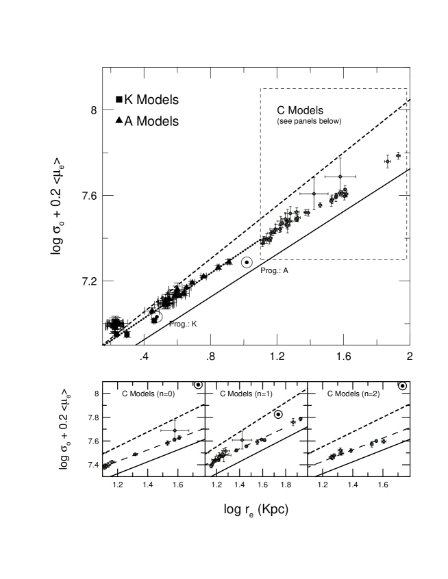
Figure 2: Results of the collapse simulations in terms of the FP parameters. The positions of the equilibrium models corresponding to the three basic sets of initial models are shown circumscribed by larger circles. The solid line gives the slope a family of homologous equilibrium systems would have in this plot, whereas the short dashed line is the best fit to the mergers products of CdCC95. For clarity the C models have been plotted separately on the three lower panels. Main (top) figure: The dotted line fits the A models. The C models are shown for direct comparison with the K and A models. The dashed square represents the area traced by the smaller panels below. Lower panels: Detailed results for the C models, where each panel shows the C models in terms of their $n$ parameter. The long dashed line fits each of the C models.

First, by examining this figure and the best fitting slopes given in Table 2 we find that the FP correlations (illustrated by the short dashed line in the figure) do not seem to be recovered by the collapsed systems. In fact, the best fitting slopes are all consistent with $\alpha=2$ which is the slope predicted by the virial equations applied to homologous systems (represented by the solid line in the figure). Second, the collapsed objects tend to cluster in the FP space variables with their location depending primarily on the initial model from which they result.

Indeed, the K models cluster in a small region of the FP space, except for two or three “hottest” collapses ($\log\beta>-0.75$), which detach from the “cluster”. This somewhat precludes any attempt to fit the resulting objects into a scaling relation. The A collapses also show this behaviour, but not as strongly as the K models. In the case of A collapses, the best fit using all the points (dotted line in the figure) gives a relation close to that expected for homologous systems ($\alpha=1.900$).

The clustered distribution of the K models is a peculiar feature among the general behaviour of the collapsed models in the FP parameter space. The K models do not “spread” along the virial plane, whereas the other models are well distributed. A naive approach to understand the reasons for this different behaviour is the following: by a combination of the energy conservation and the virial theorem, an arbitrary distribution of stars with initially zero random velocities will collapse and settle in a configuration with a radius typically a half of the initial radius. Evidently, our models do not start with such extremely “cold” conditions, since the progenitors are in fact assigned with different values of their collapse factors (the $\beta$ parameter, as described in Section 2). This should spread the models along the virial surface. However, with the abovementioned approximation in mind, it is expected that the K and A models, which have the same initial radius ($R=20$), should occupy after virialization similar locations in $\log r_{e}$, whereas the C models (initial radius $R=100$) should settle in larger $r_{e}$’s. In fact, the C models are located in the upper right region of the diagram in Fig. 2. The A and K models, on the other hand, do not occupy similar locations and distributions in the FP parameter space, although they are assigned the same collapse factors as the other models. The K and A models have different initial mass distributions, as can be seen by their different initial effective radii. It is possible that the initial central mass concentration of a given model may dynamically influence the final locations of the models within the FP space, as well as driving the models towards a more clustered distribution on the virial plane. Unfortunately, a more descriptive argument on how the dynamics could play that role is not clear at present.

The C models, quite independently from the spectral index $n$, may globally approach homologous systems. By keeping only the “coldest” C n=1 models, the resulting fit deviates from homology ($\alpha=1.070$), although the associated error bar is large ($N_{fit}=11$). In any case, these results substantially differ from those found for the set of merger simulations of CdCC95, where the FP relation is fully recovered, as can be seen by the short dashed line on Figure 2, which represents the best fit for the merger end products (slope $\alpha=1.36\pm 0.08$), as given in their paper.

One word of caution concerns the somewhat large error bars resulting from some of the fits to our collapse models in the FP parameter space, compared to that found by CdCC95 ($\delta\alpha=0.08$; the slope error quoted in CdCC95 results from a fit to $17$ models). We have confirmed that this effect results from the number of models used for the corresponding fits, which are, in some cases, small (e.g., only $10$ runs for the n=0, n=2 C models). We have increased the number of runs for the A (initially from $10$ to $22$ runs) and for the C n=1 models (from $10$ to $19$ runs) and the error bars ($\delta\alpha$’s) decreased by $\sim 40-50\%$. The general result is that the final collapsed models do not seem to follow a FP-like relation.

In order to further assertain the general homologous nature of the models, we follow the analysis of CdCC95. The virial theorem, applied to a stationary, self-gravitating system, establishes that $\langle v^{2}\rangle={GM/r_{G}}$, where $r_{G}$ is the gravitational radius (c.f. Binney & Tremaine (1987)) and $\langle v^{2}\rangle^{1\over 2}$ the three-dimensional velocity dispersion. These physical quantities can be translated into observational ones through a definition of certain kinematical-structural coefficients ($C_{r},C_{v}$), which may or may not be constants among galaxies:

$$C_{r}\equiv r_{G}/r_{e}$$ (1)

and

$$C_{v}\equiv\langle v^{2}\rangle/\sigma_{0}^{2};$$ (2)

Defining $I_{e}\equiv\eta\Sigma_{e}$, with $\eta\equiv\left({M\over L}\right)^{-1}$, and inserting the equations above into the virial relation, we find that $r_{e}=C_{vir}\eta\sigma_{0}^{2}I_{e}^{-1}$, where:

$$C_{vir}\equiv{C_{r}C_{v}\over 2\pi G}.$$ (3)

In the case of our numerical simulations, $\eta$ should be taken as a constant. We computed the final structural/kinematical virial coefficients defined above and the results are presented in Figure 3, where we plot these virial coefficients as a function of the collapse parameter. The associated errors are represented by the vertical bars and the symbols are the same of Figure 2. For the C models, we limit ourselves to the $n=1$ case, which represents the strongest deviation from homology for the “coldest” initial conditions.

Figure 3: Ratio of the virial coefficients $C_{vir}$ (upper panel), $C_{r}$ (central panel) and $C_{v}$ (lower panel) as a function of the initial condition $\log\beta$. Symbols: solid circles for the K collapses, solid triangles for the A models, and open pentagons for the C n=1 models.

We find that, in fact, the collapsed K and A models are approximately homologous among themselves, since the structural/kinematical virial coefficients do not vary considerably among them. Any residual non-homology present is due to the presence of the “hottest” collapses. On the other hand, the C ($n=1$) models may be thought of as globally homologous objects, but the virial coefficients do show some significant noise, considering the “coldest” family of collapses. This is compatible with what has previously been deduced from the FP parameter space.

4 Discussion

We designed a set of numerical experiments of dissipationless collapse of spherical models in order to investigate some possible constraints on the origin of the FP of elliptical galaxies.

First, the final objects are found at different locations on the FP parameter space, depending on the initial model. Even if the initial models have the same mass and length (e.g. $R$) scales, which is the case for the K and A models, they will occupy almost non-intersecting regions on the FP space. The central mass concentration of the initial models may have a determining influence on the final locations of the models on the FP space, for the same set of global structural-dynamical parameters (viz. $\beta$ and $R$).

Second, we found that the collapsed models do not globally populate the FP, being more compatible with homologous virialized systems. In particular, the final “coldest” C models, especially the n=1 models, tend to form a family with a deviation from homology, although the error bars are too large to confirm this effect. The C models are not only the result of a global collapse of the system, but also the product of a series of mergers of small fluctuations of smaller scales, which had the opportunity to grow depending on the initial conditions. In particular, the $n=0$ models seem to have collapsed more homogeneously, since its resulting scaling relations slope is quite similar to the K and A models, which are initially spherically symmetric objects with diferent central mass concentrations. In fact, the $n=0$ models represent a homogeneous model where small-scale noise has been added, so that sufficiently large clumps probably were not formed. This is unlike the $n=1$ and $n=2$ models, that might have resulted from mergers of significant clumps along with the main global collapse.

From the above discussion and also from the results of CdCC95, we conclude that merging may indeed be an important ingredient in forming non-homologous objects. In addition, we consider that, although “hot” collapses result in a “softer” process toward virialization (so that the relaxation mechanism of these collapses should be more closely related to the one produced by a slow merger), it is the mechanism of merging per se that drives objects towards non-homology. This is because we found that “cold” collapses from initial clumpy conditions are non-homologous, whereas the same cold collapse factors applied to more spherically symmetric systems do produce homology. From this, we also deduce that any dynamical constraints dictated by spherical symmetry in the initial conditions are not likely to have been present in the formation of elliptical galaxies, at least for those in clusters. This result is of course consistent with those found in the classical literature, where reasonably strong indications are found that “clumpy” and “cold” initial conditions are fundamental for the formation of objects similar to ellipticals (e.g. van Albada (1982), May & van Albada (1984), Merritt & Aguilar (1985), Aguilar & Merritt (1990), Londrillo, Messina & Stiavelli (1991)).

Figure 4: Field ellipticals data from de Carvalho & Djorgovski (1992) in terms of the FP parameters. The solid line is a homologous fit and the dotted line is a FP fit for the Coma cluster.

On the other hand, considering the possibility that field elliptical galaxies underwent insignificant merging episodes in their past histories (e.g. Totani & Yoshii (1998)), and assuming that their gross properties could be described by a simple, spherically symmetric collapse model, our simulations indicate that they should present a FP relation much closer to the virial expectations, compared to cluster ellipticals. Alternatively, these field elliptical galaxies could also be non-homologous objects if they collapsed from reasonably “clumpy” and “cold” initial conditions. Recently, some authors have concentrated on the analysis of the FP of field early-type galaxies, but the data is still very preliminary and precludes any firm determination of the resulting FP “tilt” for these galaxies (e.g.,van Dokkum et al. (2001), Treu et al. (1999), Pahre, Djorgovski & de Carvalho (1998), de Carvalho & Djorgovski (1992)). For instance, we directly tested the above hypothesis using the field ellipticals data from de Carvalho & Djorgovski (1992). In Figure 4, we show this data in terms of the FP parameters. The solid line is a homologous fit and the dotted line is a FP fit for the Coma cluster. The residuals show that it is not possible to verify which of the relations is the best fit due to the high dispersion of the data. The K models in our simulations are able to produce some dispersion, depending on the initial parameters (e.g. $\beta$ and/or mass), but they are not able to “move” the resulting models along any relation. We conclude that much more data is needed in order to decisively test the constraints presented by our models on the FP of field ellipticals.

Finally, we point out that our present analysis is, of course, not entirely realistic, and is based on simple one-component dissipationless models. Our conclusions should be interpreted more as a general trend to be further investigated by a larger series of higher resolution simulations. But the exercise seems to be useful in bringing out some clues that otherwise could be difficult to unravel in a more complex scenario. We intend to further refine our results adopting more realistic scenarios. Two-component models and full cosmological simulations are being currently investigated and will be the subject of a future paper.