Planets in Stellar Clusters Extensive Search. I. Discovery of 47 Low-amplitude Variables in the Metal-rich Cluster NGC 6791 with Millimagnitude Image Subtraction Photometry.

Abstract

We have undertaken a long-term project, Planets in Stellar Clusters Extensive Search (PISCES), to search for transiting planets in open clusters. As our first target we have chosen NGC 6791 – a very old, populous, metal rich cluster. In this paper we present the results of a test observing run at the FLWO 1.2 m telescope. Our primary goal is to demonstrate the feasibility of obtaining the accuracy required for planetary transit detection using image subtraction photometry on data collected with a 1 m class telescope. We present a catalog of 62 variable stars, 47 of them newly discovered, most with low amplitude variability. Among those there are several BY Dra type variables. We have also observed outbursts in the cataclysmic variables B7 and B8 (Kaluzny et al. 1997).

1 Introduction

Since antiquity mankind has wondered whether planetary systems other than our own exist. The first documented effort aimed at extrasolar planet detection was undertaken by Huygens in the XVIIth century. Starting in the 1930s, subsequent searches have been attempted, but failed to produce positive results due to insufficient measurement precision. Only recently it has become possible to obtain radial velocity measurements accurate enough to indirectly detect planets via Doppler shifts of stellar spectra of stars other than the Sun (Mayor & Queloz 1995).

To date, over 70 planets have been discovered, mainly around solar type stars. All of them were detected by radial velocity surveys (eg. Marcy et al. 2001, Noyes et al. 1997). For one of these systems, HD 209458, the transit of the planet across the host star’s disk has been observed (Charbonneau et al. 2000, Henry et al. 2000), thus demonstrating the feasibility of detecting planets this way. Several groups are currently monitoring the brightness of thousands of stars to search for planets via transits (eg. Brown & Charbonneau 1999, Quirrenbach et al. 1998). Recently, Udalski et al. (2002) discovered 46 stars with transiting low-luminosity companions. These objects may be planets, brown dwarfs or M dwarfs. A confirmation of their nature will be provided by mass determinations based on photometry combined with radial velocities from followup spectroscopic observations.

The analysis of the properties of stars with planets suggests that they are on the average significantly more metal rich than those without (Santos et al. 2001). Some studies indicate that the source of the metallicity is most likely “primordial” (Santos et al. 2001, Pinsonneault et al. 2001), while others suggest that the observed high metallicity is intrinsic only in some cases, with the more likely cause being the accretion of planetesimals onto the star (Murray & Chaboyer 2001) or the infall of giant gas planets (Lin 1997).

Although the observed lack of planets in the low metallicity ([Fe/H]$=-0.7$) globular cluster 47 Tuc (Gilliland et al. 2000) is compatible with the “primordial” metallicity scenario, the case is far from being resolved. In such dense environments as the cores of globular clusters encounters with other stars may lead to the breakup of planetary systems (Davies & Sigurdsson 2001). The study of open clusters offers the possibility of disentangling the effects of metallicity and crowding: their stellar densities are not high enough for crowding-induced disruption to be effective.

We have undertaken a long-term project, Planets in Stellar Clusters Extensive Search (PISCES), to search for transiting planets in open clusters. As our first target we have chosen NGC 6791 $[(\alpha,\delta)_{2000}=(19^{h}20.8^{m},+37^{\circ}51^{\prime})]$, a very old, extremely metal rich cluster ($\tau$=8 Gyr, [Fe/H]=+0.4; Chaboyer et al. 1999). At a distance modulus of (m-M)_V = 13.42 (Chaboyer et al. 1999) it contains about 10000 stars (Kaluzny & Udalski 1992, hereafter KU92).

In this paper we present the results of a test observing run at the FLWO 1.2 m telescope. Our aim was to demonstrate the feasibility of obtaining the required accuracy using image subtraction photometry on data collected with a 1-m class telescope needed to reliably detect transits of inner-orbit gas-giant planets with an acceptably low false alarm rate.

On clear nights we have reached the desired level of photometric precision. Unfortunately, there were few such nights during our 26 night run, which is typical for July at FLWO. Even though this dataset is not optimal for planetary transit detection, it allowed us to discover 47 new low amplitude variables, compared to 22 previously known (Kaluzny & Rucinski 1993; Rucinski, Kaluzny & Hilditch 1996, hereafter: RKH).

The paper is arranged as follows: §2 describes the observations, §3 summarizes the reduction procedure, §4 outlines the procedure of variable star selection, §5 contains the variable star catalog. Concluding remarks are found in §6.

2 Observations

The data analyzed in this paper were obtained at the FLWO 1.2 m telescope using the 4Shooter CCD mosaic with four thinned, back side illuminated AR coated Loral $2048^{2}$ CCDs (Szentgyorgyi et al. 2002). The camera, with a pixel scale of $0\farcs 333$ pixel^-1, gives a field of view of $11\farcm 4\times 11\farcm 4$ for each chip. The cluster was centered on chip 3 (Fig. 1). The data were collected during 18 nights, from July 6th to August 1st, 2001. None of the nights were photometric and most were at least partially cloudy, as this was the monsoon season. A total of $204\times 900$ s $R$ and $36\times 450$ s $V$-band exposures were obtained. The median seeing was $1\farcs 9$ in R and $2\farcs 1$ in V.

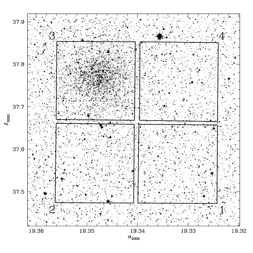
Figure 1: Digital Sky Survey image of NGC 6791 showing the field of view of the 4Shooter. The chips are numbered clockwise from 1 to 4 starting from the bottom left chip. NGC 6791 is centered on chip 3. North is up and east is to the left

3 Data Reduction

3.1 Image Subtraction Photometry

The preliminary processing of the CCD frames was performed with the standard routines in the IRAF ccdproc package.

The photometry for all stars in the field was extracted using the ISIS image subtraction package (Alard & Lupton 1998, Alard 2000) from the $R$ and $V$-band data for all four CCD chips.

ISIS is based on the fast optimal image subtraction (OIS) algorithm. In order to successfully subtract two images, it is necessary to exactly match their seeing. In OIS this is accomplished by finding a convolution kernel $Ker$ and difference in background levels $bg$ which will minimize the squared differences between both sides of the equation:

$$Im(x,y)=Ker(x,y;u,v)\otimes Ref(u,v)+bg(x,y)$$

where $Ref$ is the reference image and $Im$ is the processed image. (Alard & Lupton 1998, Wozniak 2000).

The ISIS reduction procedure consists of the following steps: (1) transformation of all frames to a common $(x,y)$ coordinate grid; (2) construction of a reference image from several best exposures; (3) subtraction of each frame from the reference image; (4) selection of stars to be photometered; (5) extraction of profile photometry from the subtracted images.

All computations were performed with the frames internally subdivided into four sections ($sub\_x=sub\_y=2$). Differential brightness variations of the background were fit with a first degree polynomial ($deg\_bg=1$). A convolution kernel varying quadratically with position was used ($deg\_spatial=2$).

An image of particularly good quality was selected as the template frame for the stellar positions. The remaining images were re-mapped to the template frame coordinate system using a second degree polynomial transform (degree=2). During this step an initial rejection of cosmic rays was also performed. A setting of 1.0 for the cosmic ray threshold (cosmic_thresh) was used.

A reference image was then constructed from 20 best images in $R$ and 15 in $V$. The constituent images were processed to match the template PSF and background level and then stacked by taking a median in each pixel to obtain a reference image virtually free of cosmic rays.

Image subtraction was then applied to all the frames. For each frame the reference image was convolved with a kernel to match its PSF and then the frame was subtracted from it. As the flux of the non-variable stars on both images should be almost identical, such objects will disappear from the subtracted image. The only remaining signal will come from variable stars.

Next comes the selection of stars for photometry. Normally at this stage the standard ISIS variable detection procedure is used. It computes a median of absolute deviations on all subtracted images and performs a simple rejection of cosmic rays and defects. This approach works very well for variables with an amplitude of at least 0.1 mag, but is much less efficient for variables of smaller amplitude. As we are interested in these latter variables we extracted photometry for all the stars on the template list, to search them for variability using more traditional methods.

Figure 2: The rms scatter of the $R$-band light curves for the best night. The left panel shows the scatter for ISIS light curves, the right panel for DAOphot. The continuous curve indicates the photometric precision limit due to Poisson noise of the star and sky brightness and the dashed ones show the 6.5 $sigma$ detection limits for 1, 1.5, 2 and 3 $R_{J}$ planets with orbital periods of 3.5 days.

A final step, not included in the ISIS image subtraction package itself, was to convert the light curves from ADU to magnitudes. For this purpose the template frames were reduced with the DAOphot/Allstar package (see Section 3.2 for details). The template instrumental magnitude $m_{tpl}$ of each star was converted into counts $c_{tpl}$, using the Allstar zeropoint of 25 mag. The light curve was then converted point by point to magnitudes $m_{i}$ by computing the total flux $c_{i}$ for a given epoch as the sum of the counts on the template $c_{tpl}$ and the counts on the subtracted template image $\Delta c_{tpl}=c_{ref}-c_{tpl}$ decreased by the counts corresponding to the subtracted image $\Delta c_{i}=c_{ref}-c_{i}$:

$$c_{i}=c_{tpl}+\Delta c_{tpl}-\Delta c_{i}$$ (1)

The flux was converted to instrumental magnitudes using the same zero point as above. To convert the photometric error $\sigma^{c}_{i}$ expressed in counts to $\sigma^{m}_{i}$ in magnitudes, we used the following relation:

$$\sigma^{m}_{i}=-2.5\log\left(\frac{c_{i}}{c_{i}+\sigma^{c}_{i}}\right)$$ (2)

3.2 Profile Photometry

Profile photometry was extracted using the DAOphot/Allstar package (Stetson 1987) from images remapped onto the template $(x,y)$ coordinate grid. This was done mainly to compare its precision to that of image subtraction photometry.

A PSF varying linearly with position on the frame was used. Stars were identified using the FIND subroutine and aperture photometry was performed with the PHOT subroutine. The same star list was used on all frames for the construction of the PSF. Of those the stars with profile errors greater than twice the average were rejected and the PSF was recomputed. This procedure was repeated until no such stars were left on the list. The PSF was then further refined on frames with all but the PSF stars subtracted from them. This procedure was applied twice. The resultant PSF was then used by Allstar in profile photometry.

The next step was to obtain a template list of stars, to be also used as the input star list for the photometry routine in ISIS. The template and the stacked reference image were reduced following the same procedure as for single frames. The stars were then subtracted from the reference image and an additional 100-200 stars undetected in the initial FIND run were hand-selected and added to the star list. Allstar was run again twice on the expanded list, which resulted in the rejection of some more objects. The star list was further cleaned by rejecting objects with $\chi>3$ and with errors too large for their magnitude. This list was used as input to Allstar on the template frame to create the final list of stars.

The final template star list was then used as input to Allstar in the fixed-position mode on each of the frames. The output profile photometry was transformed to the common instrumental system of the template image and then combined into a database. The database was created for the $R$-band images in chip 3 only.

Figure 3: The transit length (upper panel) and the probability of occurence of a transit given random inclinations (lower panel) as a function of $R$-band magnitude, plotted for periods of 1, 3.5, 5, 10 and 15 days.

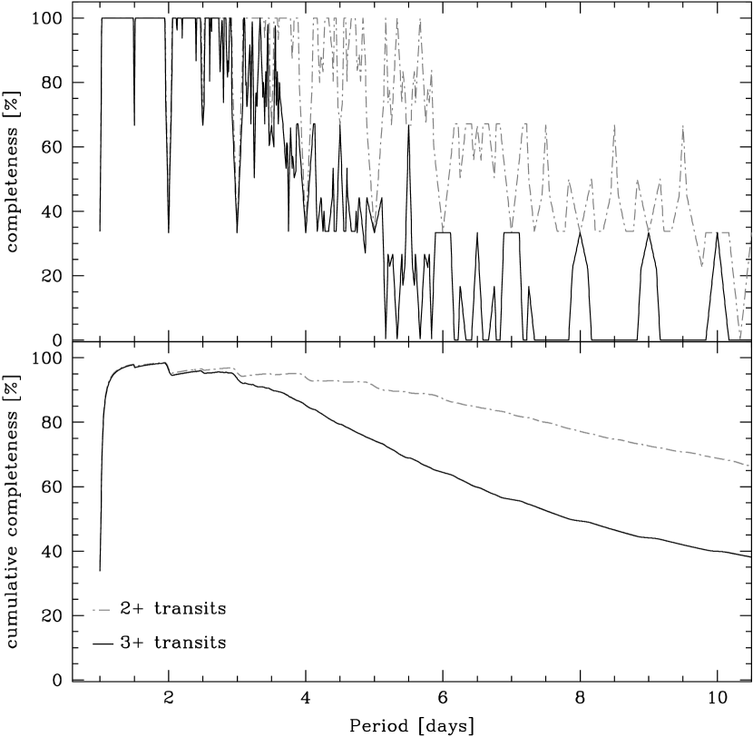
Figure 4: Detection efficiency of planetary transits as a function of their period, assuming $8^{h}$ of observations per night during 30 consecutive nights.

Figure 5: The distribution of best night residuals for 6871 stars normalized to the rms.

Figure 6: The $R$ and $V$ residuals as a function of $\vr$ for 12 stars from von Braun et al. (1998).

3.3 Implications for transit detection

In Figure 2 we plot the ISIS (left panel) and DAOphot/Allstar (right panel) time series precision as a function of magnitude for the best night. This night should be representative of the average night we expect other than during the July-August monsoon season. The time series precision was computed as the rms of the light curve, with the rejection of $3\sigma$ outliers. Only stars with light curves containing at least 22 of 23 data points are plotted. The continuous curve indicates the photometric precision limit due to Poisson noise of the star and sky brightness. The dashed curves correspond to the rms value which would yield a 6.5 $\sigma$ detection for three transits in the $R$-band, for planets with 1, 1.5, 2 and 3 $R_{J}$ and orbital period of 3.5 days, the same as for HD 209458. The curves are defined by the equation

$$rms=\sqrt{N}\frac{\Delta R}{\sigma}$$ (3)

where $N$ is the number of observations during three transits, $\Delta R$ is the $R$-band amplitude of the transit and $\sigma$ is set at 6.5. The steep fall of detection capability at the bright end is caused by the increase in radius on the subgiant branch and the 8 hour limit on the transit length set by the length of the night. The increase at the faint end is caused by the decrease of the stellar radius along the main sequence.

Not surprisingly, the overall precision is better and the scatter smaller for image subtraction photometry. This is especially well seen for the brightest stars. In the plot for image subtraction photometry 6562 (95%), 5304 (77%), 4110 (59%) and 2053 (29%) stars fall within the detection limit for transits of 3, 2, 1.5 and 1 $R_{J}$ planets, respectively.

There is a group of stars with $rms>0.1$ mag and $R<20$, with several discrepant points in the light curve caused by bad columns, which were not removed by sigma clipping. Following the approach of Udalski et al. (2002) we will set an upper limit on the $rms$ to remove such stars from the sample searched for planetary transits.

Figure 3 shows the transit length (upper panel) and the probability of occurence of a transit given random inclinations (lower panel) as a function of $R$-band magnitude, plotted for periods of 1, 3.5, 5, 10 and 15 days. The transit length is proportional to the period $P$ as $P^{\frac{1}{3}}$ and the probability of observing a transit given random inclinations, is proportional to $P^{-\frac{2}{3}}$. Both of these quantities depend on the mass, $M$, and radius, $R$, of the star as $M^{-\frac{1}{3}}R$ (Eqs (1) in Gilliland et al. 2000). The duration of the transits is of the order of 1 to 4 hours and it decreases with the magnitude of the star. For periods over $3.5$ days the probability of a transit is of the order of 10% for stars near the turnoff and it falls to 2-5% for lower main sequence stars.

Figure 4 shows the detection efficiency (upper panel) and cumulative detection efficiency (lower panel) for transiting planets with periods greater than $1^{d}$ as a function of period, assuming $8^{h}$ of observations per night during a $30$ day continuous run. The choice of the minimum period is motivated by the shortest period transiting object ($P=0.8082^{d}$) reported by Udalski et al. (2002), although it should be noted that the shortest period for a planet detected by radial velocity searches is $\sim 3$ days (HD 83443, Mayor et al. 2000). The detection efficiency for at least two transits drops below 30% at $P\sim 9^{d}$ (upper panel, dot-dashed line) and for at least three transits at $P\sim 5^{d}$ (solid line). Such temporal coverage would enable us to observe three or more transits for 50% of all transiting planets with periods between $1$ and $7.8$ days (lower panel, solid line). A 50% efficiency for the detection of at least two transits is reached at a period of $15.7$ days (dot-dashed line).

The distribution of best night residuals for 6871 stars, normalized to the rms, is shown in Fig. 5. Only stars with at least 22 out of 23 data points were included in the histogram. The distribution of the residuals is well-fit by a Gaussian distribution with $\sigma=0.96$.

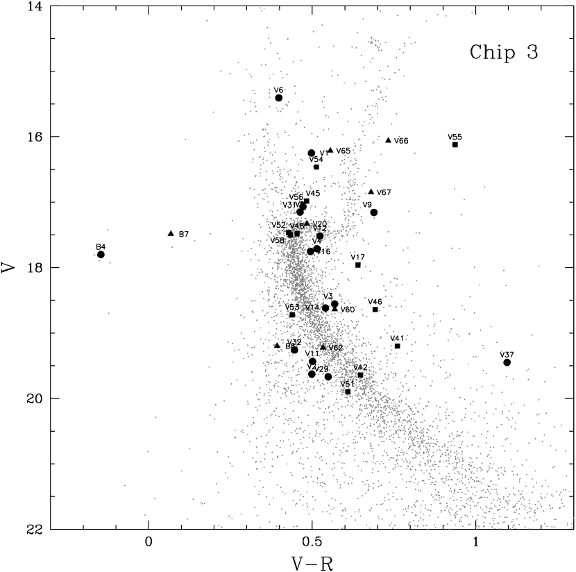
Figure 7: $V/\vr$ color-magnitude diagram (CMD) for chip 3, centered on NGC 6791. Eclipsing binaries are plotted with circles, other periodic variables with squares and miscellaneous variables with triangles.

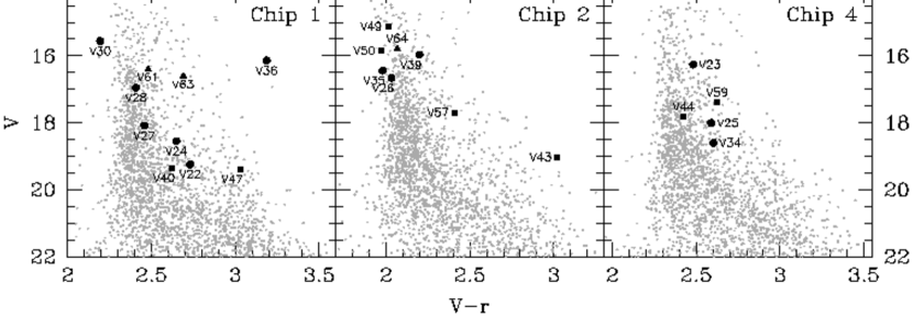
Figure 8: $V/V-r$ CMDs for chips 1, 2 and 4. Eclipsing binaries are plotted with circles, other periodic variables with squares and miscellaneous variables with triangles.

3.4 Calibration

None of the nights in our observing run were photometric, thus we were forced to rely on other, indirect sources of calibration.

The $R$-band photometry in chip 3 was calibrated from the photometry for 12 of the 14 red giant branch (RGB) stars published by von Braun et al. (1998). One of the stars could not be identified on our template and another one, much redder than the others (R4, $\vr=1.355$) was rejected because it was a clear outlier in both $R$ and $V$. Due to the small number of stars and a very limited color baseline, only an offset was determined. The residuals, with an rms scatter of 0.014 mag, are shown in the upper panel of Fig. 6. The $R$-band photometry for chips 1, 2 and 4 was left uncalibrated, as they contain no stars with calibrated $R$-band photometry.

A similar comparison was made for the $V$-band magnitudes of the 12 RGB stars and there seems to be a trend with color (lower panel of Fig. 6) and magnitude, as those two quantities are correlated for RGB stars. A trend in magnitude is also present for stars with $V<17$ in comparison with data of Kaluzny & Rucinski (1995; hereafter KR95), but is not seen in case of the KU92 photometry. Since the KR95 data cover parts of all four chips and the offset is in good agreement with the von Braun et al. (1998) photometry (to $0.005$ mag), we have used offsets from the KR95 photometry to bring the instrumental magnitudes to the standard system.

In Figures 7 and 8 we present the $V/\vr$ CMDs for chip 3 and chips 1, 2, 4, respectively. The CMD for chip 3, centered on the cluster, shows a well defined main sequence (MS) down to $V\sim 20$, a subgiant branch (SGB), a red giant branch and a red clump at $V\sim 14.5$, $\vr\sim 0.7$. The blue stars, noted by KU92, are also present at $\vr<0$. The CMDs for the remaining chips consist in large proportion of disk stars; only an indication of the upper MS is discernible.

3.5 Astrometry

Equatorial coordinates were determined for the $R$-band template star lists, expanded with the variables with no $R$-band photometry. The transformation from rectangular to equatorial coordinates was derived using 734, 729, 1058 and 657 transformation stars from the USNO A-2 catalog (Monet et al. 1996) in chips 1 through 4, respectively. The average difference between the catalog and the computed coordinates for the transformation stars was $0\farcs 14$ in right ascension and $0\farcs 12$ in declination.

4 Variability Search

4.1 Selection of Variables

To select candidate variable stars we have employed the variability index J defined by Stetson (1996). Below we present only a summary of the method; the reader is referred to the original paper for details.

The variability index J is computed as follows:

$$J=\frac{\sum^{n}_{k=1}w_{k}\mathrm{sgn}(P_{k})\sqrt{|P_{k}|}}{\sum^{n}_{k=1}w_{k}}$$

where the user has defined n pairs of observations, i and j, to be considered, each with a weight $w_{k}$. In our case, observations separated by less than 0.03 days were treated as a pair. A weight $w_{k}=1$ was assigned to pairs of observations ($i(k)\neq j(k)$) and $w_{k}=0.25$ to single observations ($i(k)=j(k)$). $P_{k}$ is the product of the normalized residuals of the two observations, i and j, constituting the k-th pair:

$$P_{k}=\left\{\begin{array}[]{ll}\delta_{i(k)}\delta_{j(k)},&\mathrm{if~{}}i(k)\neq j(k)\\ \delta_{i(k)}^{2}-1,&\mathrm{if~{}}i(k)=j(k)\end{array}\right.$$

and $\delta$ is the magnitude residual of a given observation from the average, scaled by the standard error:

$$\delta=\sqrt{\frac{n}{n-1}}\frac{v-\bar{v}}{\sigma_{v}}$$

The final variability index was multiplied by a factor $\sum w/w_{max}$, where $w_{max}$ is the total weight of a star if it were measured on all images.

We are aware that this approach is not optimal for detecting planetary transits and a better method based on the matched-filter algorithm is under development. Recently, Udalski et al. (2002) used this technique to identify 46 transiting planet candidates. They report that their implementation was very sensitive even to single transit events and produced virtually no spurious detections.

We believe the choice of the algorithm was not critical for the dataset analized here. Due to the poor weather conditions during most of the observing run and the resulting decreased photometric accuracy on some nights and uneven temporal coverage, we did not expect to find planetary transits.

Figure 9: The light curves of the 30 eclipsing binaries. Crosses indicate standard $R$ magnitude, points - instrumental.

Figure 9: Continued.

4.2 Period Determination

To search for periodicities we have used the method introduced by Schwarzenberg-Czerny (1996), employing periodic orthogonal polynomials to fit the observations and the analysis of variance statistic to evaluate the quality of the fit.

If observations $X$ consist of the sum of signal $F$ and noise $E$: $X_{k}=F_{k}+E_{k}$, then the analysis of variance statistic $\Theta(\omega)$ is defined as:

$$\Theta(\omega)\equiv\frac{\hat{Var}\{F\}}{\hat{Var}\{E\}}=\frac{(K-2N-1)\sum_{n=0}^{2N}|c_{n}^{2}|}{2N[(X,X)-\sum_{n=0}^{2N}|c_{n}^{2}|]}$$

where 2N is the order of the complex polynomial (corresponding to a Fourier series of N harmonics), K is the number of observations and $c_{n}$ are the coefficients of the orthonormal polynomial $\Psi_{N}(z)=\sum_{n=0}^{N}c_{n}\Phi_{n}(z)$, where $\Phi_{N}(z)=\sum_{n=0}^{N}a_{n}^{(N)}z^{n}$ is the base. For the details of the method the reader is referred to the Schwarzenberg-Czerny (1996) paper.

5 Variable Star catalog

We have found 62 variables in all four chips, 47 of them new ones (24 in chip 3): 30 eclipsing binaries, 21 other periodic variables and 11 miscellaneous ones. Their $R$-band light curves are shown in Figures 9, 10 and 11 and parameters listed in Tables 1, 2 and 3, respectively. The variables are also plotted on CMDs for their respective chips [Figs 7 (chip 3) and 8 (chips 1, 2, 4)]. Eclipsing binaries are marked with circles, other periodic variables with squares and miscellaneous variables with triangles.

We have recovered 18 of the 22 previously known variables. The missing four are V7 and V8, which are outside of our feld of view, and V13 and V19, which are saturated in the $R$-band data. The light curves of the long period detached eclipsing binaries V10, V18 and V21 are also not shown, as we have not observed any eclipses for them.

We have reobserved the W UMa type eclipsing variables V1-V6. We confirm the longer of the two possible periods found for V5 by RKH. This variable shows unequal maxima, as noted previously by RKH. The shape of the light curve is seen to have changed: in our data the variable attains higher maximum brightness at phase 0.25 (between the primary and the secondary eclipse) and in the RKH data at phase 0.75. The light curve of V4 shows a similar change: the maxima are almost equal now, while in the RKH data they were clearly uneven. The variability of the maxima is probably due to changing starspots on the surface of one or both of the components, like in RS CVn type binaries. We have discovered six new W UMa type systems in chips 1, 2 and 4, V22-V28. One of them, V23, also shows unequal maxima.

V6 exhibits extremely small amplitudes of 0.1 mag in $R$ and $V$, considering its flat-bottomed minima. Such light curve shape would indicate an inclination angle close to $90^{\circ}$ and an extremely small mass ratio for the binary components ($q<0.05$, Rucinski 1993). A comparison with the 0.15 mag amplitude light curve in Kaluzny et al. (1993) strongly suggests that this variable is blended in our data. This is confirmed by the elongated appearance of the star on our reference frame.

Another short period eclipsing variable, V29, does not seem to be a contact system judging by the narrowness of the primary eclipse. On the CMD it is located below the main sequence, together with V2 and V11. It is most likely a field star behind the cluster.

B4, one of the blue stars identified by KU92, shows brightness variations with an amplitude of 0.05 mag. We have phased the light curve with a period of 0.8 days, so that it displays two minima and two maxima. B4 might be a non-eclipsing binary with brightness modulations due to ellipsoidal variations or a reflection effect. An argument in favor of this interpretation comes from a study of the radial velocities of a sample of 70 sdBs which indicates that 45% of them are post-common envelope binaries with periods of the order of a few hours to a few days (Saffer, Green & Bowers 2000). The period for B4 is consistent with this period range.

The binary nature of B4 is interesting from the point of view of the origin of hot subdwarfs in metal rich clusters. Binary evolution has been suggested as one of the possible formation mechanisms of such objects (Moehler 2001).

Figure 10: The light curves of the 21 other periodic variables. Crosses indicate standard $R$ magnitude, points - instrumental.

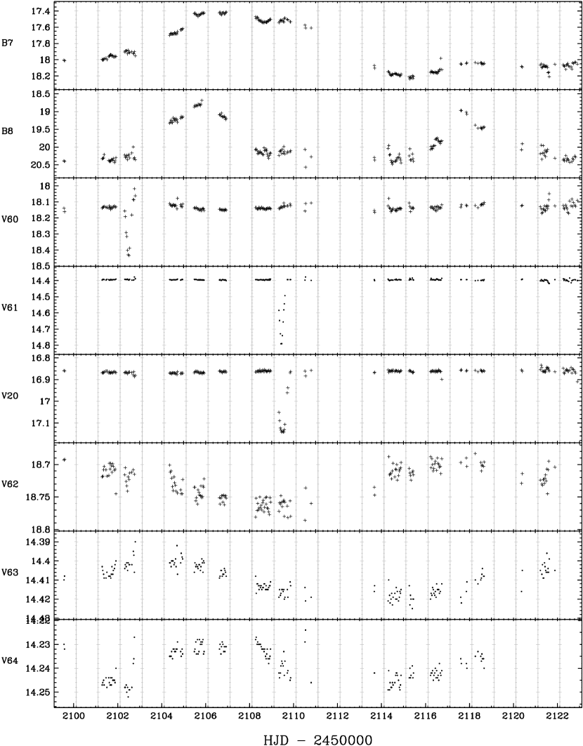
Figure 11: The light curves of the 11 miscellaneous variables. Crosses indicate standard $R$ magnitude, points - instrumental.

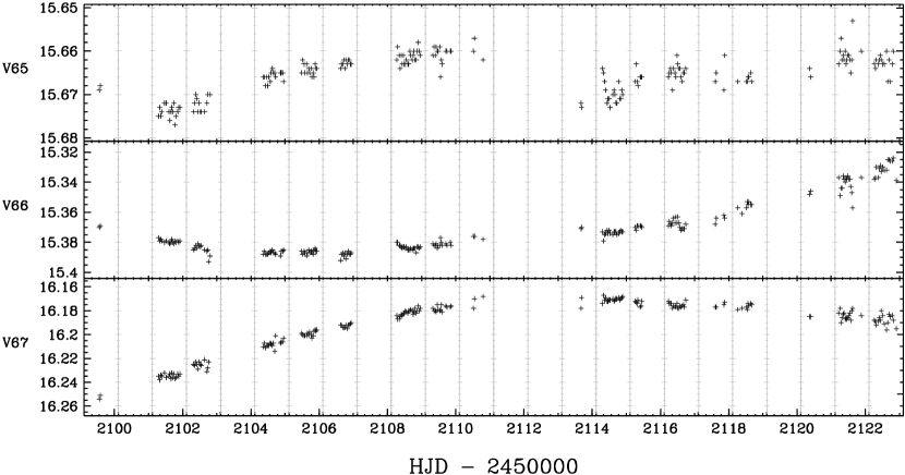
Figure 11: Continued.

We have also found some variables which could either be EB type eclipsing binaries or ellipsoidal variables, as most have amplitudes smaller than 0.1 mag. Among them are V14 and V16 with newly derived periods. The new variables which belong to this type are V30, V31, V33, V34, V36 and possibly V37 and V38. During one of the nights V37 seems to have undergone a UV Ceti-like outburst with an amplitude of 0.1 mag (Fig 9). This variable is also very red, with V R=1.1 and most likely not a cluster member.

We have reobserved the RS CVn type eclipsing binary V9. The shape of the S-wave does not seem to have changed significantly from the one observed by RKH in 1996.

We have derived periods for the EA type eclipsing binaries V11, V12. For the detached eclipsing system V20 we have observed only one eclipse. Three new such sytems, V35, V60 and V61, were observed as well. A period for V35 was derived, as it appears that one of the eclipses was observed twice. Other possible EA type binaries are V32 and V39.

In addition to eclipsing binaries and ellipsoidal variables we have also discovered periodic variables which seem to be of different nature. The newly phased variable V17, as well as the new variables V40-V44, V46, V47, V51, V53 are most likely BY Dra type variables – rotating spotted late type dwarfs. On the CMDs they are located in the vicinity of the lower MS ($V>18.5$) or redward of it. Some are probably not cluster members. V40-V42 and possibly V46 exhibit small humps between the maxima. Similar behavior has been observed for other BY Dra type variables, eg. CC Eri (Amado et al. 2000). We have also considered the possibility that V40-V42 are field RR Lyrae stars. Despite the similarity in the light curve shape and period, this interpretation seems unlikely because of their small amplitudes.

The remaining periodic variables are brighter than $V=18$. The nature of their variability is unclear. These variables are spread throughout the CMDs. V48, V52 and V58 seem to be located at the cluster turnoff, and V45, V54, V56, V49 and V50 above it. V55, significantly redder than the RGB stars, is probably not a cluster member. The variables V57 and V59 seem to be located redward of the turnoff. V59 exibits quite a high amplitude of 0.3 mag.

Among the miscellaneous variables there are two especially interesting ones: the cataclysmic variables B7 (V15) and B8 (Kaluzny et al. 1997). B7 was observed to undergo a 0.6 mag outburst while in its high state. B8 showed two dwarf-novae type outbursts, the first one with an amplitude of 2 mag and duration of about 5 days and a second, slightly fainter one.

Five of the six other miscellaneous variables, V63-V67, are located above the cluster turnoff. V62 appears to be located on the MS. Most of the bright variables seem to show long period or quasi-periodic variability. V66 and V67, located $\sim 0.1$ mag redward of the RGB, display variations on a longer timescale than the other variables.

6 Conclusions

In this paper we have demonstrated the feasibility of obtaining photometry accurate enough to detect planets through transits in open clusters with 1 m class telescopes. The analysis of the data collected for this purpose resulted in the discovery of 47 new low amplitude variables, compared to 22 previously known (Kaluzny & Rucinski 1993, RKH).

The first stage of our project will be to obtain for this and several other clusters continuous observations with a 1-m class telescope for about $\sim$30 nights under very good observing conditions. The photometry will be obtained in two bands, $R$ and $V$, to allow us to differentiate between planetary transits and blended eclipsing binaries. Planetary transits should be gray, as the planet does not contribute any measurable light to the system, while the superposition of an eclipsing binary with another star will show a change in color during the eclipse.

In the next stage better light curves will be obtained with a 2 m class telescope for selected planet transit candidates. Using radial velocity measurements derived from spectroscopic observations with a 6-10 m class telescope it will be possible to distinguish planetary and brown dwarf transits from grazing eclipses by main sequence companions. A precision of 1 km s^-1 will enable us to identify and reject stars with companions above 0.0075 M_⊙ ($\sim 8$ M_J).

Table 1: Eclipsing binaries in NGC 6791

ID	$\alpha_{2000}$	$\delta_{2000}$	P [d]	$R_{max}$	$V_{max}$	$A_{R}$	$A_{V}$
V22	19.338527	37.508317	0.2452	16.507∗	19.239	0.794	0.862
V1	19.346557	37.742245	0.2677	15.744	16.223	0.327	0.328
V23	19.338612	37.787813	0.2718	13.772∗	16.255	0.072	0.064
V2	19.354874	37.766766	0.2732	19.125	19.623	0.176	0.281
V24	19.332915	37.595612	0.2759	15.897∗	18.546	0.200	0.209
V25	19.328430	37.713417	0.2773	15.414∗	18.004	0.540	0.525
V6	19.350753	37.813595	0.2790	15.008	15.397	0.093	0.097
V26	19.345806	37.561879	0.2836	14.626∗	16.659	0.210	0.221
V5	19.346259	37.813295	0.3126	16.687	17.149	0.055	0.060
V3	19.354378	37.769396	0.3176	17.986	18.550	0.087	0.128
V4	19.348395	37.806623	0.3256	17.194	17.710	0.109	0.088
V27	19.336295	37.649081	0.3318	15.624∗	18.082	0.698	0.651
V28	19.328836	37.591770	0.3720	14.540∗	16.949	0.474	0.454
V29	19.354795	37.751474	0.4365	19.117	19.653	0.248	0.359
B4	19.353583	37.764289	0.7973	17.945	17.797	0.054	0.064
V11	19.342582	37.804615	0.8822	18.911	19.424	0.462	0.395
V30	19.328617	37.501978	1.1692	13.359∗	15.554	0.023	0.030
V12	19.345259	37.849032	1.5336	16.989	17.508	0.241	0.238
V31	19.350685	37.785921	1.5362	16.597	17.067	0.024	0.040
V32	19.341003	37.787297	2.0958	18.809	19.242	0.140	0.174
V33	19.344394	37.731803	2.3663	10.796∗	$\cdots$	0.095	$\cdots$
V34	19.335880	37.736360	2.4112	15.993∗	18.597	0.175	0.197
V35	19.345574	37.511924	2.5741	14.454∗	16.435	0.220	0.219
V36	19.332336	37.570224	2.6772	12.950∗	16.138	0.047	0.092
V9	19.346634	37.777067	3.1723	16.463	17.146	0.173	0.154
V37	19.355069	37.851982	3.2199	18.385	19.436	0.080	0.291
V38	19.351024	37.768325	3.8856	18.276	$\cdots$	0.097	$\cdots$
V16	19.352108	37.802683	4.5010	17.258	17.749	0.085	0.097
V39	19.350133	37.639703	7.5928	13.764∗	15.964	0.068	0.053
V14	19.347684	37.756898	11.2962	18.075	18.615	0.071	0.107

Note. — ^∗ Instrumental magnitudes

Table 2: Other periodic variables in NGC 6791

ID	$\alpha_{2000}$	$\delta_{2000}$	P [d]	$R_{max}$	$V_{max}$	$A_{R}$	$A_{V}$
V40	19.327499	37.617002	0.3979	16.714∗	19.340	0.060	0.070
V41	19.347492	37.806861	0.4816	18.436	19.201	0.040	0.040
V42	19.350057	37.714872	0.5068	18.993	19.641	0.060	0.070
V43	19.344330	37.641893	0.7521	16.003∗	19.026	0.040	0.100
V44	19.326974	37.694940	2.2505	15.383∗	17.809	0.030	0.030
V45	19.346126	37.701676	4.5776	16.499	16.982	0.010	0.020
V46	19.355274	37.798960	5.1482	17.947	18.642	0.040	0.050
V47	19.327533	37.536375	5.5803	16.345∗	19.378	0.050	0.070
V48	19.352077	37.718522	5.6025	17.028	17.477	0.020	0.020
V49	19.341914	37.614271	5.6483	13.102∗	15.114	0.010	0.010
V50	19.343115	37.517920	5.7341	13.865∗	15.836	0.010	0.020
V17	19.344137	37.817929	6.1752	17.317	17.958	0.030	0.040
V51	19.353380	37.748568	6.6443	19.294	19.892	0.090	0.100
V52	19.355798	37.772043	7.0550	17.039	17.465	0.010	0.010
V53	19.350232	37.743195	7.4704	18.283	18.720	0.020	0.020
V54	19.355196	37.726814	8.4208	15.950	16.460	0.010	0.010
V55	19.356229	37.841641	11.0277	15.185	16.120	0.000	0.010
V56	19.345907	37.763584	11.5791	16.567	17.034	0.010	0.020
V57	19.349417	37.518655	13.0809	15.278∗	17.689	0.020	0.030
V58	19.354038	37.801263	13.6219	17.069	17.498	0.030	0.030
V59	19.339303	37.806090	14.4738	14.759∗	17.385	0.150	0.170

Note. — ^∗ Instrumental magnitudes

Table 3: Other periodic variables in NGC 6791

ID	$\alpha_{2000}$	$\delta_{2000}$	$R_{max}$	$V_{max}$	$A_{R}$	$A_{V}$
V61	19.328572	37.485425	13.903∗	16.383	0.470	0.383
V63	19.327780	37.495899	13.913∗	16.603	0.029	0.035
V64	19.353181	37.498769	13.707∗	15.773	0.024	0.085
V62	19.350848	37.731070	18.686	19.215	0.098	0.095
B8	19.343257	37.747859	18.803	19.117	1.951	2.991
V66	19.352340	37.748699	15.324	16.056	0.067	0.034
V20	19.348416	37.759650	16.846	17.327	0.314	0.293
V60	19.350193	37.762524	18.067	18.633	0.346	0.217
V65	19.347908	37.791815	15.658	16.211	0.018	0.025
B7	19.352056	37.799037	17.418	17.476	0.880	0.883
V67	19.351021	37.801035	16.167	16.845	0.079	0.096

Note. — ^∗ Instrumental magnitudes

References

- (1) Alard, C., Lupton, R. 1998, ApJ, 503, 325
- (2) Alard, C. 2000, A&AS, 144, 363
- (3) Amado, P. J., et al. 2000, A&A, 359, 159
- (4) Brown, T. M., Charbonneau, D. 1999, AAS, 195, 110907
- (5) Chaboyer, B., Green, E. M., Liebert, J. 1999, AJ, 117, 1360
- (6) Charbonneau, D., Brown, T. M., Latham, D. W., Mayor, M. 2000, ApJ, 529, L45
- (7) Davies, M. B. & Sigurdsson, S. 2001, MNRAS, 324, 612
- (8) Gilliland, R. L., et al. 2000, ApJ, 545, L47
- (9) Henry, G. W., Marcy, G. W., Butler, R. P., & Vogt, S. S. 2000, ApJ, 529, L41
- (10) Kaluzny, J., Ruciński, S. M. 1995, A&AS, 98, 477 (KR95)
- (11) Kaluzny, J., Ruciński, S. M. 1993, MNRAS, 265, 34
- (12) Kaluzny, J., Stanek, K. Z., Garnavich, P. M. & Challis, P. 1997, ApJ, 491, 153
- (13) Kaluzny, J., Udalski, A. 1992, Acta Astronomica, 42, 29 (KU92)
- (14) Lin, D. N. C. 1997, ASP Conf. Ser., 121, 321
- (15) Marcy, G. W., et al. 2001, ApJ, 556, 296
- (16) Mayor, M., Queloz, D. 1995, Nature, 378, 355
- (17) Mayor, M., et al. 2000, in Planetary Systems in the Universe: Observations, Formation and Evolution, ASP Conf. Ser.
- (18) Moehler, S. 2001, PASP, 113, 1162
- (19) Monet, D., et al. 1996, USNO-A2.0, (U.S. Naval Observatory, Washington DC).
- (20) Murray, N., Chaboyer, B. 2002, ApJ, 566, 442
- (21) Noyes, R. W. 1997, ApJ, 483, L111
- (22) Pinsonneault, M. H., DePoy, D. L., Coffee, M. 2001, ApJ, 556, L59
- (23) Quirrenbach, A., & EXPORT Team 1998, AAS, 193, 9806
- (24) Ruciński, S. M., Kaluzny, J., Hilditch, R. W. 1996, MNRAS, 282, 705 (RKH)
- (25) Ruciński, S. M. 1993, PASP, 105, 1433
- (26) Saffer, R. A., Green, E. M., & Bowers, T. 2001, ASP Conf. Ser. 226: 12th European Workshop on White Dwarfs, 408
- (27) Santos, N. C., Israelian, G., Mayor, M. 2001, A&A, 373, 1019
- (28) Schwarzenberg-Czerny, A. 1996, ApJ, 460, L107
- (29) Stetson, P. B. 1996, PASP, 108, 851
- (30) Stetson, P. B. 1987, PASP, 99, 191
- (31) Szentgyorgyi, A. H. et al. 2002, in preparation
- (32) Udalski, A., et al. 2002, Acta Astronomica, submitted (astro-ph/0202320)
- (33) von Braun, K., Chiboucas, K., Minske, J. K., Salgado, J. F. 1998, PASP, 110, 810
- (34) Wozniak, P. R. 2000, Acta Astronomica, 50, 421