Multiple Peaks in the CMB

Alessandro  Melchiorri¹

¹ Denys Wilkinson Building, University of Oxford, Keble Road, Oxford, OX1 3RH, UK.

Recent measurements of the Cosmic Microwave Background Anisotropy have provided evidence for the presence of oscillations in the angular power spectrum. These oscillations are a wonderful confirmation of the standard cosmological scenario and allow us to derive constraints on many cosmological, astrophysical and inflationary parameters. If the discovery is confirmed by future experiments, opportunities may appear, for example, to constrain dark energy, variations in fundamental constants and neutrino physics.

PRESENTED AT

COSMO-01
Rovaniemi, Finland,
August 29 – September 4, 2001

1 Introduction

In the last $2$ years important progress has been made in the study of the Cosmic Microwave Background (CMB) Anisotropies.

With the TOCO$-97/98$ ([129],[107]) and Boomerang-$97$ ([100]) experiments a firm detection of the first peak in the CMB anisotropy angular power spectrum has been obtained. The presence of this peak is generally expected in models of structure formation with a nearly-scale invariant spectrum of primordial perturbations like the one produced after inflation. In the framework of adiabatic Cold Dark Matter (CDM) models, the position, amplitude and width of this peak provide strong supporting evidence for the inflationary predictions of a low curvature (flat) universe and a scale-invariant primordial spectrum ([51], [104], [125]).

A first analysis of a small fraction of data from the BOOMERANG $1998/1999$ Long Duration Ballooning (BOOM/LDB) campaign ([16], [91]) and of observations from the MAXIMA experiment ([69], [6]) further confirmed the presence of this feature at high significance. However, the finding of a suppressed second peak in the CMBR anisotropy resulted in a rather large value for the baryon density, $\Omega_{b}h^{2}=0.032^{+0.005}_{-0.004}$ at $68\%$ CL [81], while the experimental data on primordial ${}^{4}He$ and $D$ abundances, prefer smaller values, $\Omega_{b}h^{2}=0.020{\pm}0.002$ ([29]) (see also [5],[97]). Many authors addressed the issue of this tension between the determination of $\Omega_{b}h^{2}$ from CMBR data and Standard Big Bang Nucleosynthesis (SBBN) [128, 96, 57, 74, 83, 36].

The new experimental data from BOOMERANG ([111]) and DASI ([68]) have refined the data at larger multipole and now clearly suggest the presence of a second peak in the spectrum and a smaller value for the baryonic fraction, in agreement with SBBN. Moreover, this result confirms the model prediction of acoustic oscillations in the primeval plasma and shed new light on various cosmological and inflationary parameters ([17], [135], [117]). The new results from MAXIMA ([93], [122]) are of lower precision, but are consistent with both DASI and BOOMERANG.

This paper is organized as follows: Section II is a brief introduction about why we expect oscillations in the CMB spectrum. In Section III I will discuss the statistical significance of the peaks measured by BOOMERANG, DASI and MAXIMA and their location and amplitude. In section IV I will review the implications for the cosmological parameters in the framework of the standard CDM model of structure formation. In section V I will discuss some non-standard aspect of parameter extraction. Finally, in section VI, I will give my conclusions.

2 The acoustic oscillations in the CMB anisotropy angular power spectrum

2.1 The power spectrum.

The anisotropy with respect to the mean temperature $\Delta T=T-T_{0}$ of the CMB sky in the direction ${\bf n}$ measured at time $t$ and from the position $\vec{x}$ can be expanded in spherical harmonics:

$${\Delta T\over T_{0}}({\bf n},t,\vec{x})=\sum_{\ell=1}^{\infty}\sum_{m=-\ell}^{m=\ell}a_{\ell m}(t,\vec{x})Y_{\ell m}({\bf n})~{},$$ (1)

If the fluctuations are Gaussian all the statistical information is contained in the $2$-point correlation function. In the case of isotropic fluctuations, this can be written as:

$$\left\langle{\Delta T\over T_{0}}({{\bf n}_{1}}){\Delta T\over T_{0}}({{\bf n}_{2}})\right\rangle={1\over 4\pi}\sum_{\ell}(2\ell+1)C_{\ell}P_{\ell}({\bf n}_{1}\cdot{\bf n}_{2})~{}.$$ (2)

where the average is an average over ”all the possible universes” i.e., by the ergodic theorem, over $\vec{x}$. The CMB power spectrum $C_{\ell}$ are the ensemble average of the coefficients $a_{\ell m}$,

$$C_{\ell}=\langle|a_{\ell m}|^{2}\rangle~{}.$$

Since it is impossible to measure ${\Delta T\over T_{0}}$ in every position in the universe, we cannot do an ensemble average. This introduces a fundamental limitation for the precision of a measurement (the cosmic variance) which is important especially for low multipoles. If the temperature fluctuations are Gaussian, the $C_{\ell}$ have a chi-square distribution with $2\ell+1$ degrees of freedom and the observed mean deviates from the ensemble average by

$${{\Delta C_{\ell}}\over C_{\ell}}=\sqrt{2\over 2\ell+1}~{}.$$ (3)

Moreover, in a real experiment, one never obtain complete sky coverage because of the limited amount of observational time (ground based and balloon borne experiments) or because of galaxy foreground contamination (satellite experiments). All the telescopes also have to deal with the noise of the detectors and are obviously not sensitive to scales smaller than the angular resolution. For a given an experiment, the accuracy of reconstruction of the power spectrum can be approximately given as [86]:

$${{\Delta C_{\ell}}\over C_{\ell}}\simeq\sqrt{2\over(2\ell+1)f_{sky}}\left(1+{{\sigma^{2}_{pixel}\Omega_{pixel}}\over C_{\ell}}\exp[\ell^{2}\sigma^{2}_{beam}]\right)~{}.$$ (4)

where $f_{sky}$ is the sky coverage, $\sigma_{beam}$ is the angular resolution, $\sigma_{pixel}$ the experimental noise per pixel and $\Omega_{pixel}$ is the area per pixel.

2.2 Theoretical predictions. Inflation vs. Topological Defects.

Acoustic oscillations in the CMB angular spectrum have been predicted since long time from simple assumptions about scale invariance and linear perturbation theory ([113], [124], [140], [133], [22]). The physics of these oscillations and their dependence on the various cosmological parameters has been described in great detail in many reviews (see e.g. [80], [79], [139], [20], [45], [106]). Here I will just outline the basic principles and spend a few words on models based on topological defects that do not predict oscillations.

Since the CMB fluctuations are small, applying linear perturbation theory to the Friedman metric is justified. For a cosmic fluid consisting of radiation, massless neutrinos, baryons, cold dark matter and a cosmological constant, we can the write down the linear perturbation equations (in Fourier space). In the most general case, for each wave vector $\bf k$ they are of the form

$${\bf D}X={\cal S}~{},$$ (5)

where $X$ is a vector containing all the random perturbation variables, $\bf D$ is a deterministic linear first order differential operator and ${\cal S}$ is a random source term which consists of linear combinations of the energy momentum tensor of possible external sources of perturbations such as topological defects. More details can be found, e.g. in Ref. [46], [47].

In general, for inflationary perturbations ${\cal S}=0$ and the solutions are determined entirely by the random initial conditions, $X({\bf k},t_{\rm in})$. Practically, scale-invariant perturbations are induced in the metric only during the inflationary epoch by quantum fluctuations of the inflaton field. After that, no new perturbations are produced in the universe and everything evolves according to the linearized perturbation equations.

For inflationary models $X({\bf k},t_{\rm in})$ is then a set of Gaussian random variables and hence their statistical properties are entirely determined by the spectra $\cal P$ (the Fourier transforms of the two point functions),

$$\langle X_{i}((t_{\rm in},{\bf k})\ X_{j}^{*}((t_{\rm in},{\bf k}^{\prime})\rangle\equiv{\cal P}_{ij}({\bf k})\delta({\bf k}-{\bf k}^{\prime})~{}.$$ (6)

Here the Dirac delta is a consequence of statistical homogeneity which we want to assume for the random process leading to the initial perturbations. In general, for density inflationary perturbations, ${\cal P}\sim k^{n_{S}}$ where the spectral index $n_{S}$ is equal to $1$ for scale-invariance.

Let $A_{i}(k,t)$ be the solution with initial condition $X_{j}(k,t_{\rm in})$. The spectra of the solution with initial ’spectrum’ given by Eq. (6) is then today just

$$\langle X_{i}((t_{0},{\bf k})\ X_{j}^{*}((t_{0},{\bf k}^{\prime})\rangle=A_{i}(k,t_{0})A_{j}^{*}(k,t_{0}){\cal P}_{ij}(k)\delta({\bf k}-{\bf k}^{\prime})~{}.$$

Therefore, if $A_{i}$ is oscillating, e.g. as a function of $kt$ because of some physical process between $t_{\rm in}$ and $t_{0}$, so will $\langle|X_{i}|^{2}\rangle$.

This is exactly our case: on sub-horizon scales, prior to recombination, photons and baryons form a tightly coupled fluid that performs acoustic oscillations driven by the gravitational potential. These acoustic oscillations define a structure of peaks in the CMB angular power spectrum that is measured today.

Let us, for example, consider the density fluctuations $\delta$ in the baryon-photon fluid during the radiation dominated epoch. In this case we have $w=p/\rho\simeq 1/3$ equal to the adiabatic sound speed $c_{s}^{2}={\dot{p}/\dot{\rho}}\simeq 1/3$ and $\delta$ follows the wave equation:

$$\ddot{\delta}+k^{2}{\delta\over 3}={k^{2}\over 3}(\Phi-\Psi)$$ (7)

where $\Phi$ and $\Psi$ are the Bardeen potentials  [7], and the dots are derivatives respect to the time $\eta$. In our case $\Phi\simeq-\Psi\simeq const$. On very large, super-horizon scales, $k\eta\ll 1$, $\delta$ remains constant. Once $k\eta>1$ $\delta$ begins to oscillate like an acoustic wave.

If adiabatic perturbations have been created during an early inflationary epoch, they all start oscillating in phase. At the moment of recombination, when the photons become free and the acoustic oscillations stop, the perturbations of a given wave length thus all have the same phase. As each given wave length is projected to a fixed angular scale on the sky, this leads to a characteristic structure of peaks in the CMB power spectrum.

However, if the source term $\cal S$ does not vanish, the randomness of the source term enters at all times and the situation is different.

In this case, Equation (5) can be solved by means of a Green’s function, ${\cal G}(t,t^{\prime})$, in the form

$$X_{j}(t_{0},{\bf k})=\int_{t_{in}}^{t_{0}}\!dt{\cal G}_{jl}(t_{0},t,{\bf k}){\cal S}_{l}(t,{\bf k})~{}.$$ (8)

Power spectra or, more generally, quadratic expectation values of the form $\langle X_{j}(t_{0},{\bf k})X_{l}^{*}(t_{0},{\bf k})\rangle$ are then given by

$$\langle X_{j}(t_{0},{\bf k})X_{l}^{*}(t_{0},{\bf k})\rangle=\int_{t_{in}}^{t_{0}}\!dt\int_{t_{in}}^{t_{0}}\!dt^{\prime}{\cal G}_{jm}(t_{0},t,{\bf k}){\cal G}^{*}_{ln}(t_{0},t^{\prime},{\bf k})\langle{\cal S}_{m}(t,{\bf k}){\cal S}_{n}^{*}(t^{\prime},{\bf k})\rangle~{}.$$ (9)

The only information about the source random variable which we really need in order to compute power spectra are therefore the unequal time two point correlators (see e.g.  [2, 114, 3, 50, 46]

$$\langle{\cal S}_{m}(t,{\bf k}){\cal S}_{n}^{*}(t^{\prime},{\bf k})\rangle~{}.$$ (10)

In the case of topological defects or more general non homogeneous distributions of matter, $\cal S$ is given by a function quadratic in the defect field, which itself obeys highly non-linear evolution equations. The non-linearity of the time evolution of the source term has several important consequences. Even though time evolution is deterministic, different Fourier modes mix due to non-linearity, and the randomness in one mode ’sweeps’ into the other modes.

Therefore, fluctuations of a given wave number $k$ are in general not in phase, and the distinctive series of acoustic peaks present in inflationary models is blurred into one ’broad hump’.

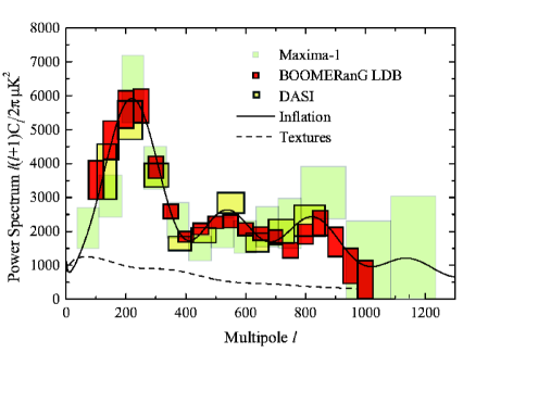
In Figure 1 we plot the $2$ (very different) theoretical predictions one for an inflationary model and one for a model based on numerical simulations of global textures taken from [46]. Global textures can be considered a good representative for the models with non linear sources. The cosmological parameters are assumed to be the same.

As we can see, when non-linearities are present as in the textures case, decoherence dominates and the oscillations in the CMB spectrum are severely damped. Also plotted in the figure are the recent data from the BOOMERanG and DASI experiments. It is clear from the picture that while the inflationary scenario is in good agreement with the data, the texture model is ruled out at high significance.

This is an important result: structure formation theories based on non-linear external sources fail to match the current data, and defects as only responsible mechanism for structure formation can reasonably be ruled out.

However, before going to parameter extraction, is important to asses how well the current data are in agreement with the underlying theoretical model and with the presence of acoustic oscillations.

3 Are there acoustic oscillations in the CMB power spectrum ?

Figure 1: BOOMERanG, DASI and MAXIMA data togheter with an inflationary model and a global textures model.

On April 30th 2001, at the same time, $3$ different teams, Boomerang [111], DASI [68] and MAXIMA [93] reported a detection of multiple features in the CMB angular power spectrum. Before discussing the statistical significance of these features, let me briefly review the various experiments.

3.1 The BOOMERanG experiment.

BOOMERanG is a scanning balloon experiment aimed at producing accurate and high signal/noise maps of the CMB sky and constraining the power spectrum in the $50<\ell<1000$ range. The BOOMERanG experiment has been described in [116] and [15]. All the relevant informations about the collaboration can be found in the ’official’ websites: http://oberon.roma1.infn.it/boom and http://www.physics.ucsb.edu/b̃oomerang/.

The BOOMERanG group carried out a long duration flight (December 1998/ January 1999) called the Antarctica or LDB flight. Before this, there was a ’test flight’ on North America from which the first power spectrum results were released ([100], [104], [116]). From the test flight a $\sim 4000$ $16^{\prime}$ pixel map at $150GHz$ produced a firm detection of a first peak in the CMB angular power spectrum.

For the antarctica flight, coverage of $4$ frequencies with $16$ bolometers in total were available. BOOMERanG LDB measured $8$ pixels in the sky simultaneously . Four pixels feature multiband photometers ($150$, $240$ and $410$ GHz), two pixels have single-mode, diffraction limited detectors at $150$ GHz and two pixels have single-mode, diffraction limited detectors at $90$ GHz. The NEP of these detectors is below $200\mu K_{CMB}\sqrt{s}$ at $90$, $150$ and $240$ GHz and the angular resolution ranges from $12$ to $18$ arcminFWHM.

The istrument was flown aboard a stratospheric balloon at $38Km$ of altitude to avoid the bulk of atmospheric emission and noise. During a long duration balloon flight of $\sim 11$ days carried out by NASA-NSBF around Antarctica in $1999$, BOOMERanG mapped $\sim 1800$ square degrees in a region of the sky with minimal contamination from the galaxy.

The most recent analysis of the BOOMERanG data has been presented in [111]. The observations taken from $4$ detectors at $150$ GHz in a dust-free ellipsoid central region of the map ($1.8\%$ of the sky) have been analyzed using the methods of ([23], [76], [118]). The gain calibration are obtained from observations of the CMB dipole.

The CMB angular power spectrum, estimated in $19$ bands centered between $\ell=50$ to $\ell=1000$ is shown in Figure 1. The error bars on the $y$ axis are correlated at about $\sim 10\%$. A first peak is clearly evident at $\ell\sim 200$ and $2$ subsequent peaks can be see in the figure. Not shown in the figure is an additional $10\%$ calibration error (in $\Delta T$) and the uncertainty in the beam size ($12.9^{\prime}\pm 1.4^{\prime}$).

Calibration error does not affect the shape of the power spectrum, producing only an overall shift in amplitude.

On the contrary, since the beam resolution affects the $C_{\ell}$ spectrum according to the Eq. (4), a small uncertainty $\Delta\sigma^{2}_{beam}=\sigma^{2}_{beam}-(\sigma_{beam}^{\prime})^{2}$ in the telescope beam produce a correlated $\ell$-dependent ’calibration error’ of $\sim(1+\ell^{2}\Delta\sigma^{2}_{beam})C_{\ell}$ ([27])

The beam uncertainty can change the relative amplitude of the peaks, but cannot introduce features in the spectrum.

3.2 The DASI experiment.

The DASI experiment is a ground based compact interferometer constructed specifically for observations of the CMB. A description of the instrument can be found in [68] and [94]. and all the relevant information about the team can be obtained from the DASI website:http://astro.uchicago.edu/dasi/.

The specific advantage of interferometers is in reducing the effects of atmospheric emission [90]. DASI is composed of $13$ element interferometers with correlator operating from $26$ to $36$ GHz. The baseline of DASI cover angular scales from $15^{\prime}$ to $1.4^{o}$.

Interferometry is a technique that differs in many fundamental ways from those used by BOOMERanG and other map-making CMB experiments. Interferometers directly sample the Fourier transform of the sky brightness distribution and the CMB power spectrum can be computed without going through the map making process. In this sense, the DASI result provides a real independent observation of the CMB angular spectrum.

The most recent analysis of the DASI data has been presented in [68]. The observations have been taken over $97$ days from the South-Pole during the austral summer at frequencies between $26$ and $36$ GHz. The calibration was obtained using bright astronomical sources.

The CMB angular power spectrum estimated in $9$ bands between $\ell=100$ to $\ell=900$ is also shown in Figure 1. There is a $\sim 20\%$ correlation between the data points. Not shown in the figure is an $\sim 8\%$ calibration error, while the beam error is negligible. The DASI team found no evidence for foregrounds other than point sources (which are the dominant foregrounds at those frequencies (see e.g. [126], [127])). Nearly $30$ point sources have been detected in the DASI data while a statistical correction has been made for residual point sources that were too faint to be detected.

3.3 The MAXIMA experiment.

MAXIMA-I is another balloon experiment, similar in many aspects to BOOMERang but not long-duration. A description of the instrument can be found in [93] and all the relevant informations about the team can be obtained from the MAXIMA website: http://cosmology.berkeley.edu/group/cmb/. In the latest analysis ([93]) the data from $3$, $150$, GHz very sensitive bolometers has been analyzed in order to produce a $3^{\prime}$ pixelized map of about $10$ by $10$ degrees. The previous analysis of about the same data based on a $5^{\prime}$ pixelization ([69]) has therefore been extended to $\ell=1235$. The map-making method used by the MAXIMA team is extensively discussed in [123]. The data are calibrated using the CMB dipole.

The MAXIMA-I datapoints are also shown in Figure 1. The error bars are correlated at level of $\sim 10\%$. The $\sim 4\%$ calibration error is not plotted in the figure. The beam/pointing errors are of order of $\sim 10\%$ at $\ell=1000$ (see [93]).

3.4 Features in the CMB power spectrum.

Figure 2: Phenomenological fit to the BOOMERanG, DASI and Maxima data. Picture taken from [43]

Before going on to parameter extraction, it is important to adopt a phenomenological approach and try to quantify how well the present data provide evidence for multiple and coherent oscillations. Fits to the CMB data with phenomenological functions have been already extensively used in the past (see e.g. [119], [121], [88]). More recently, similar analyses have been carried out, using parabolas ([17], [49]) or more elaborate oscillating functions with a well defined frequency and phase ([43]).

Since the first peak is evident, the statistical significance of the secondary oscillations is now of greater interest. In [17] the BOOMERanG data bins centered at $450<\ell<1000$ were analyzed. Using a Bayesian approach, a linear fit $C_{\ell}^{T}=C_{A}+C_{B}\ell$ is rejected at near $2\sigma$ confidence level. Also in [17], using a parabolic fit to the data, interleaved peaks and dips were found at $\ell=$ $215\pm 11$, $431\pm 10$, $522\pm 27$, $736\pm 21$ and $837\pm 15$ with amplitudes of the features $5760^{+344}_{-324}$, $1890^{+196}_{-178}$, $2290^{+330}_{-290}$, $1640^{+500}_{-380}$, and $2210^{+900}_{-640}$ $\mu K^{2}$, correspondingly. The reported significance of the detection is $1.7\,\sigma$ for the second peak and dip, and $2.2\,\sigma$ for the third peak.

The evidence for oscillations in the MAXIMA data has been carefully studied in [122]. While there is no evidence for a second peak, the power spectrum shows excess power at $\ell\sim 860$ over the average level of power at $411\leq\ell\leq 785$ on the $95\%$ confidence level. Such a feature is consistent with the presence of a third acoustic peak.

In [49] the BOOMERanG, DASI and MAXIMA data were included in a similar analysis. Both DASI and MAXIMA confirmed the main features of the Boomerang CMB power spectrum: a dominant first acoustic peak at $\ell\sim 200$, DASI shows a second peak at $\ell\sim 540$ and MAXIMA-I exhibits mainly a ’third peak’ at $\ell\sim 840$.

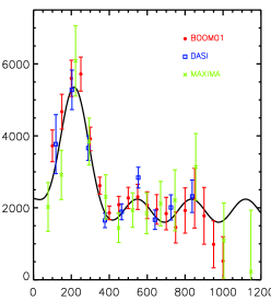
Finally and more recently, in [43] a different analysis was made, based on a function that smoothly interpolates between a spectrum with no oscillations and one with oscillations. Again, within the context of this different phenomenological model, a $2\sigma$ presence for secondary oscillations was found. In Figure 2 the best phenomenological fit to the data from [43] is reported. As we can see, the oscillations are clearly present in the BOOMERanG and DASI data and are compatible with the MAXIMA data.

4 Consequences for Cosmology

Since the observations are, at the very least, compatible with acoustic oscillations, we can make the assumption of inflationary perturbations and undertake a parameter estimation.

Constraining the parameters of the model with the present CMB data can be regarded as a further test for the consistency of the scenario, since one can then compare the results with those obtained by independent methods and/or under different theoretical assumptions.

In principle, the CDM scenario of structure formation based on adiabatic primordial fluctuations can depend on more than $11$ parameters.

However for a first analysis, it is useful to restrict ourselves to just $5$ parameters: the tilt of primordial spectrum of perturbations $n_{S}$, the optical depth of the universe $\tau_{c}$, the density in baryons and dark matter $\omega_{b}=\Omega_{b}h^{2}$ and $\omega_{dm}=\Omega_{dm}h^{2}$ and the shift parameter ${\cal R}$ which is related to the geometry of the universe through (see [53], [103]):

$${\cal R}=2\sqrt{|\Omega_{k}|/\Omega_{m}}/\chi(y)$$ (11)

where $\Omega_{m}=\Omega_{b}+\Omega_{dm}$, $\Omega_{k}=1-\Omega_{m}-\Omega_{\Lambda}$, the function $\chi(y)$ is $y$, $\sin(y)$ or $\sinh(y)$ for flat, closed and open universes respectively and

$$y=\sqrt{|\Omega_{k}|}\int_{0}^{z_{dec}}{[\Omega_{m}(1+z)^{3}+\Omega_{k}(1+z)^{2}+\Omega_{\Lambda}]^{-1/2}dz}.$$ (12)

Figure 3: Confidence contours in the $\Omega_{M}-\Omega_{\Lambda}$ and $\Omega_{b}h^{2}-n_{S}$ planes. Picture taken from [17].

The restriction of the analysis to only $5$ parameters can be justified in several way: First, a reasonable fit to the data can be obtained with no additional parameters. Second, constraints on these parameters provide a test of the scenario: the value of the baryon density $\Omega_{b}h^{2}$ can be compared with the values obtained from Big Bang Nucleosynthesis; $\Omega_{dm}h^{2}$ must be significantly different from zero since a purely baryonic model doesn’t match the observed galaxy clustering; $\Omega=1$ and $n_{S}\sim 1$ are general predictions of the inflationary scenario.

Let us consider the results from BOOMERanG, DASI and MAXIMA separately, joint analysis have been reported in, for example, ([135]) and ([43]).

In Fig. 3 we plot the likelihood contours in the $\Omega_{M}-\Omega_{\Lambda}$ and $\Omega_{b}h^{2}-n_{S}$ planes from the BOOMERanG experiment as reported in [17]. Since the quantity ${\cal R}$ depends on $\Omega_{\Lambda}$ and $\Omega_{M}$ the CMB constraints on this parameter can be plotted on this plane. As we can see from the left panel in the figure the data strongly suggest a flat universe (i.e. $\Omega=\Omega_{M}+\Omega_{\Lambda}=1$). From the latest BOOMERanG data one obtains $\Omega=1.02\pm 0.06$ ([111]).

The inclusion of complementary datasets in the analysis breaks the angular diameter distance degeneracy in $\cal R$ and provides evidence for a cosmological constant at high significance. Adding the Hubble Space Telescope constraint on the Hubble constant $h=0.72\pm 0.08$ ([62], information from galaxy clustering and from luminosity distance of type Ia supernovae gives ([111]) $\Omega_{\Lambda}=0.62_{-0.18}^{+0.10}$, $\Omega_{\Lambda}=0.55_{-0.09}^{+0.09}$ and $\Omega_{\Lambda}=0.73_{-0.07}^{+0.10}$ respectively.

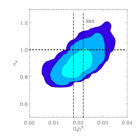
Also interesting is the plot of the likelihood contours in the $\Omega_{b}h^{2}-n_{S}$ plane. These $2$ parameters are crucial in the determination of the relative amplitude of the peaks and the power on subdegree angular scales. Namely, increasing the baryon density, increases the difference between the first and second peak. Decreasing the scalar spectral index has the same effect since we are removing power from small scales and adding it to large angular scales. Therefore, some sort of degeneracy exists among these parameters that can however be broken by measuring the power around the $3$rd peak. The presence of the degeneracy is exemplified by the elongation of the likelihood contours along the $\omega_{b}-n_{S}$ direction. The present data, however, already provide enough information about the power on the $3$rd peak and the degeneracy is partially broken.

The most important result from the right panel of Figure 3 is that the present BOOMERanG data is in beautiful agreement with both a nearly scale invariant spectrum of primordial fluctuations, as predicted by inflation, and the value for the baryon density $\omega_{b}=0.020\pm 0.002$ predicted by Standard Big Bang Nucleosynthesis (see e.g. [29]).

Figure 4: CDM model vs purely baryonic dark matter models. Picture taken from [19].

An increase in the optical depth $\tau_{c}$ after recombination by reionization (see e.g. [67] for a review) or by some more exotic mechanism damps the amplitude of the CMB peaks. Even if degeneracies with other parameters such as $n_{S}$ are present (see e.g. [14]) the BOOMERanG data provides the upper bound $\tau_{c}<0.3$.

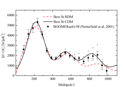
The amount of non-baryonic dark matter is also constrained by the CMB data with $\Omega_{dm}h^{2}=0.13\pm 0.04$ at $68\%$ c.l. ([111]). The presence of power around the third peak is crucial in this sense, since it cannot be easily accommodated in models based on just baryonic matter (see e.g. [19], [65], [102] and references therein). In Fig.4 we plot the BOOMERanG data with the best fit purely baryonic (BDM) and CDM model (picture taken from [19]). As we can see, BDM models fail to reproduce the observed power at $\ell\geq 700$.

Furthermore, under the assumption of flatness, we can derive important constraints on the age of the universe $t_{0}$ given by:

$$t_{0}=9.8Gy\int_{0}^{1}{{ada\over{[\omega_{m}a+\omega_{\Lambda}a^{4}]^{1/2}}}}$$ (13)

Figure 5: Age constraint from CMB compared with independent estimates. Picture taken from [59].

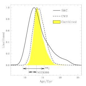
In Figure 5 we compare the BOOMERanG constraint on age with other independent results obtained from stellar populations in bright ellipticals ([59]), ²³⁸U age-measurement of an old halo star in our galaxy ([32]) and age the of the oldest halo globular cluster in the sample of Salaris & Weiss ([120]). As we can see all four methods give completely consistent results, and enable us to set rigorous bounds on the maximum and minimum ages that are allowed for the universe, $t_{0}=14\pm 1$ GYrs ([59], [111],[87]).

The results from the DASI experiment have been extensively reported in [117] and are perfectly consistent with the BOOMERanG results. Pryke et al. report $\Omega=1.04\pm 0.06$, $n_{s}=1.01^{0.08}_{0.06}$, $\Omega_{b}h^{2}=0.022^{0.004}_{0.003}$ and $\Omega_{dm}h^{2}=0.14\pm 0.04$.

The MAXIMA team reported similar compatible constraints in [122]: $\Omega=0.9{+0.18\atop-0.16}$ and $\Omega_{b}h^{2}=0.033{\pm 0.13}$ at $2\sigma$ c.l.. However the MAXIMA data is not good enough to put strong constrains on the spectral index $n_{S}$ and the optical depth $\tau_{c}$ because of the degeneracy between the $2$ parameters.

5 Non-Standard Aspects of Parameter extraction

Even if the present CMB observations can be fitted with just $5$ parameters it is interesting to extend the analysis to other parameters allowed by the theory. Here I will just summarize a few of them and discuss how well we can constrain them and what the effects on the results obtained in the previous section would be.

5.1 Gravity Waves

The metric perturbations created during inflation belong to two types: scalar perturbations, which couple to the stress-energy of matter in the universe and form the “seeds” for structure formation and tensor perturbations, also known as gravitational wave perturbations. Both scalar and tensor perturbations contribute to CMB anisotropy. In the recent CMB analysis by the BOOMERanG and DASI collaborations, the tensor modes have been neglected, even though a sizable background of gravity waves is expected in most of the inflationary scenarios. Furthermore, in the simplest models, a detection of the GW background can provide information on the second derivative of the inflaton potential and shed light on the physics at $\sim 10^{16}Gev$ (see e.g. [77]).

The shape of the $C^{T}_{\ell}$ spectrum from tensor modes is drastically different from the one expected from scalar fluctuations, affecting only large angular scales (see e.g. [35]). The effect of including tensor modes is similar to just a rescaling of the degree-scale $COBE$ normalization and/or a removal of the corresponding data points from the analysis.

This further increases the degeneracies among cosmological parameters, affecting mainly the estimates of the baryon and cold dark matter densities and the scalar spectral index $n_{S}$ ([105],[84], [135], [52]).

The amplitude of the GW background is therefore weakly constrained by the CMB data alone, however, when information from BBN, local cluster abundance and galaxy clustering are included, an upper limit of about $r=C_{2}^{T}/C_{2}^{S}<0.5$ is obtained.

5.2 Scale-dependence of the spectral index.

The possibility of a scale dependence of the scalar spectral index, $n_{S}(k)$, has been considered in various works (see e.g. [89], [33], [98], [38]). Even though this dependence is considered to have small effects on CMB scales in most of the slow-roll inflationary models, it is worthwhile to see if any useful constraint can be obtained. Allowing the power spectrum to bend erases the ability of the CMB data to measure the tensor to scalar perturbation ratio and enlarge the uncertainties on many cosmological parameters.

Recently, Covi and Lyth ([34]) investigated the two-parameter scale-dependent spectral index predicted by running-mass inflation models, and found that present CMB data allow for a significant scale-dependence of $n_{S}$. In Hannestad et al. ([72], [73]) the case of a running spectral index has been studied, expanding the power spectrum $P(k)$ to second order in $ln(k)$. Again, their result indicates that a bend in the spectrum is consistent with the CMB data.

Furthermore, phase transitions associated with spontaneous symmetry breaking during the inflationary era could result in the breaking of the scale-invariance of the primordial density perturbation. In [9], [66] and [134] the possibility of having step or bump-like features in the spectrum has also been considered.

While much of this work was motivated by the tension between the initial release of the data and the baryonic abundance value from BBN, a sizable feature in the spectrum is still compatible with the latest CMB data ([54]).

5.3 Quintessence

The discovery that the universe’s evolution may be dominated by an effective cosmological constant [63] is one of the most remarkable cosmological findings of recent years. One candidate that could possibly explain the observations is a dynamical scalar “quintessence” field. One of the strongest aspects of quintessence theories is that they go some way towards explaining the fine-tuning problem, that is why the energy density producing the acceleration is $\sim 10^{-120}M_{pl}^{4}$. A vast range of “tracker” (see for example [142, 26]) and “scaling” (for example [138], [58]) quintessence models exist which approach attractor solutions, giving the required energy density, independent of initial conditions. The common characteristic of quintessence models is that their equations of state, $w_{Q}=p/\rho$, vary with time while a cosmological constant remains fixed at $w_{Q=\Lambda}=-1$ (see e.g. [18]). Observationally distinguishing a time variation in the equation of state or finding $w_{Q}$ different from $-1$ will therefore be a success for the quintessential scenario. Quintessence can also affect the CMB by acting as an additional energy component with a characteristic viscosity. However any early-universe imprint of quintessence is strongly constrained by Big Bang Nucleosynthesis with $\Omega_{Q}(MeV)<0.045$ at $2\sigma$ for temperatures near $T\sim 1Mev$ ([11], [141]).

In [12] we have combined the latest observations of the CMB anisotropies and the information from Large Scale Structure (LSS) with the luminosity distance of high redshift supernovae (SN-Ia) to put constraints on the dark energy equation of state parameterized by a redshift independent quintessence-field pressure-to-density ratio $w_{Q}$.

The importance of combining different data sets in order to obtain reliable constraints on $w_{Q}$ has been stressed by many authors (see e.g. [115], [78],[137]), since each dataset suffers from degeneracies between the various cosmological parameters and $w_{Q}$ . Even if one restricts consideration to flat universes and to a value of $w_{Q}$ constant in time then the SN-Ia luminosity distance and position of the first CMB peak are highly degenerate in $w_{Q}$ and $\Omega_{Q}$, the energy density in quintessence.

Varying $w_{Q}$ on the angular power spectrum of the CMB anisotropies has just $2$ effects. First, since the inclusion of quintessence changes the overall content of matter and energy, the angular diameter distance of the acoustic horizon size at recombination will be altered.

In flat models (i.e. where the energy density in matter is $\Omega_{M}=1-\Omega_{Q}$), this creates a shift in the peaks’ positions in the angular spectrum by

$${\cal R}^{-1}={1\over 2}\sqrt{(1-\Omega_{Q})}\int_{0}^{z_{dec}}[(1-\Omega_{Q})(1+z)^{3}+\Omega_{Q}(1+z)^{3(1+w_{Q})}]^{-1/2}dz.$$ (14)

It is important to note that the effect is completely degenerate in the interplay between $w_{Q}$ and $\Omega_{Q}$. Furthermore, it does not add any new features beyond those produced by the presence of a cosmological constant [53], and it is not particularly sensitive to further time dependencies of $w_{Q}$.

Second, the time-varying Newtonian potential after decoupling will produce anisotropies at large angular scales through the Integrated Sachs-Wolfe (ISW) effect. The curve in the CMB angular spectrum on large angular scales depends not only on the value of $w_{Q}$, but also on its variation with redshift. This effect, however, will be difficult to disentangle from the same effect generated by a cosmological constant, especially in view of the affect of cosmic variance and/or gravity waves on the large scale anisotropies.

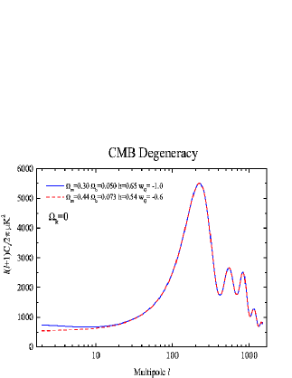
In order to emphasize the importance of degeneracies among all of these parameters while analyzing the CMB data, we plot in Figure $6$ some degenerate spectra, obtained by keeping the physical density in matter $\Omega_{M}h^{2}$, the physical density in baryons $\Omega_{b}h^{2}$ and ${\cal R}$ fixed. As we can see from the plot, models degenerate in $w_{Q}$ can easily be constructed. However the combination of CMB data with other different datasets can break the mentioned degeneracies.

Figure 6: CMB power spectra and the angular diameter distance degeneracy. The models are computed assuming flatness, $\Omega_{k}=1-\Omega_{M}-\Omega_{Q}=0$). The Integrated Sachs Wolfe effect on large angular scale slightly breaks the degeneracy. The degeneracy can be broken with a strong prior on $h$. Picture taken from [12].

Figure 7: The likelihood contours in the ($\Omega_{M}$, $w_{Q}$) plane, with the remaining parameters taking their best-fitting values for the joint CMB+SN-Ia+LSS analysis described in the text. The contours correspond to 0.32, 0.05 and 0.01 of the peak value of the likelihood, which are the 68%, 95% and 99% confidence levels respectively. Picture taken from [12].

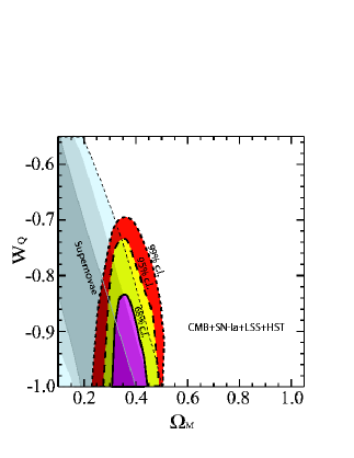
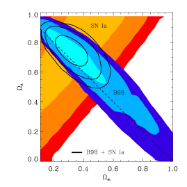
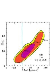
In Figure 7 we plot likelihood contours in the ($\Omega_{M}$, $w_{Q}$) plane for the joint analyses of CMB+SN-Ia+HST+LSS data together with the contours from the SN-Ia dataset only. Proceeding as in [104], we attribute a likelihood to a point in the ($\Omega_{M}$, $w_{Q}$) plane by finding the remaining parameters that maximize it. We then define our $68\%$, $95\%$ and $99\%$ contours to be where the likelihood falls to $0.32$, $0.05$ and $0.01$ of its peak value, as would be the case for a two dimensional multivariate Gaussian. As we can see, the combination of the datasets breaks the luminosity distance degeneracy and suggests the presence of dark energy with high significance. Furthermore, the new CMB results provided by Boomerang and DASI improve the constraints from previous and similar analysis (see e.g., [115],[21]), with $w_{Q}<-0.85$ at $68\%$ c.l.. Our final result is then perfectly in agreement with the $w_{Q}=-1$ cosmological constant case and gives no support to a quintessential field scenario with $w_{Q}>-1$.

5.4 CMB, Big Bang Nucleosynthesis and Neutrinos

As we saw in the previous section, the SBBN $95\%$ CL region, corresponding to $\Omega_{b}h^{2}=0.020{\pm}0.002$ ($95\%$ c.l.), has a large overlap with the analogous CMBR contour. This fact, if it will be confirmed by future experiments on CMB anisotropies, can be seen as one of the greatest success, up to now, of the standard hot big bang model.

SBBN is well known to provide strong bounds on the number of relativistic species $N_{\nu}$. On the other hand, Degenerate BBN (DBBN), first analyzed in Ref. [41, 61, 13, 82], gives very weak constraint on the effective number of massless neutrinos, since an increase in $N_{\nu}$ can be compensated by a change in both the chemical potential of the electron neutrino, $\mu_{\nu_{e}}=\xi_{e}T$, and $\Omega_{b}h^{2}$. Practically, SBBN relies on the theoretical assumption that background neutrinos have negligible chemical potential, just like their charged lepton partners. Even though this hypothesis is perfectly justified by Occam razor, models have been proposed in the literature [36, 1, 39, 40, 31, 99, 101, 60], where large neutrino chemical potentials can be generated. It is therefore an interesting issue for cosmology, as well as for our understanding of fundamental interactions, to try to constrain the neutrino–antineutrino asymmetry with the cosmological observables. It is well known that degenerate BBN gives severe constraints on the electron neutrino chemical potential, $-0.06\leq\xi_{e}\leq 1.1$, and weaker bounds on the chemical potentials of both the $\mu$ and $\tau$ neutrino, $|\xi_{\mu,\tau}|\leq 5.6\div 6.9$ [82], since electron neutrinos are directly involved in neutron to proton conversion processes which eventually fix the total amount of ${}^{4}He$ produced in nucleosynthesis, while $\xi_{\mu,\tau}$ only enters via their contribution to the expansion rate of the universe.

The CMB power spectrum is greatly affected by changes in $N_{\nu}$, the amount of relativistic particles. First of all, changing $N_{\nu}$ changes the epoch of equality. Secondly, the shift parameter $\cal R$ is changed as ([25]):

$${\cal R}=2\left(1-\frac{1}{\sqrt{1+z_{dec}}}\right)\frac{\sqrt{|\Omega_{k}|}}{\Omega_{m}}\frac{1}{\chi(y)}\left[\sqrt{\Omega_{rel}+\frac{\Omega_{m}}{1+z_{dec}}}-\sqrt{\Omega_{rel}}\right]$$ (15)

where now

$$y=\sqrt{|\Omega_{k}|}\int_{0}^{z_{dec}}dz{[\Omega_{rel}(1+z)^{4}+\Omega_{m}(1+z)^{3}+\Omega_{k}(1+z)^{2}+\Omega_{\Lambda}]^{-1/2}}.$$

Finally, in the acoustic peaks region, the different radiation content at decoupling by variation of the ratio $\Omega_{\gamma}/\Omega_{rel}$ induces a larger early ISW effect, which boosts the height of the first peak with respect to the other acoustic peaks.

Combining the DBBN scenario with the bound on baryonic and radiation densities allowed by CMBR data, it is possible to obtain stronger constraints on all the parameter of the model. Such an analysis was previously performed in ([57], [96], [70], [112]) using the first data release of BOOMERanG and MAXIMA ([16], [69]). We recall that the neutrino chemical potentials contribute to the total neutrino effective degrees of freedom $N_{\nu}$ as

$$N_{{\nu}}=3+\Sigma_{\alpha}\left[\frac{30}{7}\left(\frac{\xi_{\alpha}}{\pi}\right)^{2}+\frac{15}{7}\left(\frac{\xi_{\alpha}}{\pi}\right)^{4}\right]\,.$$ (16)

Notice that in order to get a bound on $\xi_{\alpha}$ we have here assumed that all relativistic degrees of freedom, other than photons, are given by three (possibly) degenerate active neutrinos.

Figure 8: The $95\%$ CL contours for degenerate BBN (dot-dashed (green) line), new CMB results with just the age prior, $t>11$gyr (full (red) line), and with just the SN1a prior (dashed (blue) line). The combined analysis corresponds to the filled regions. Marginalization leads to the bound $\Omega_{b}h^{2}=0.020{\pm}0.0035$ and $N_{\nu}<7$, both at $95\%$, for DBBN+CMB+SN. The dotted (green) line is the $95\%$ CL allowed by SBBN. Picture taken from [75].

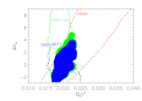
Figure 8 summarizes our main results with the new CMB data, reported in [75] for the DBBN scenario. We plot the $95\%$ CL contours allowed by DBBN (dot-dashed (green) line), together with the analogous $95\%$ CL region coming from the CMB data analysis, with only weak age prior, $t_{0}>11$gyr (full (red) line).

Finally, the solid contour (light, red) is the $95\%$ CL region of the joint product distribution ${\cal L}\equiv{\cal L}_{DBBN}$${\cdot}{\cal L}_{CMB}$. The main new feature, with respect to the results of Ref. [57] is that the resolution of the third peak shifts the CMB likelihood contour towards smaller values for $\Omega_{b}h^{2}$, so when combined with DBBN results, it singles out smaller values for $N_{\nu}$. In fact from our analysis we get the bound $N_{\nu}\leq 8$, at $95\%$ CL, which translates into the new bounds $-0.01\leq\xi_{e}\leq 0.25$, and $|\xi_{\mu,\tau}|\leq 2.9$, sensibly more stringent than what can be found from DBBN alone.

A similar analysis can also be performed combining CMBR and DBBN data with the Supernova Ia data [63], which strongly reduces the degeneracy between $\Omega_{m}$ and $\Omega_{\Lambda}$. At $95\%$ C.L. we find $\Delta N_{\nu}<7$, corresponding to $-0.01\leq\xi_{e}\leq 0.22$ and $|\xi_{\mu,\tau}|\leq 2.6$.

Compatible results have been obtained in similar analyses ([85],[71]).

Some caution is naturally necessary when comparing the effective number of neutrino degrees of freedom from BBN and CMB, since they may be related to different physics. In fact the energy density in relativistic species may change from the time of BBN ($T\sim MeV$) to the time of last rescattering ($T\sim eV$). It is therefore interesting to further investigate the bounds on this parameter from CMB alone and see how the inclusion of a free $N_{\nu}$ can affect the results on parameter extraction.

Figure 9: Effects of a background of relativistic particles on the parameters estimated from CMB observations. Picture taken from [25].

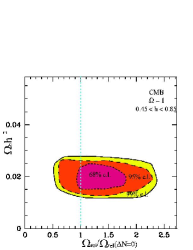
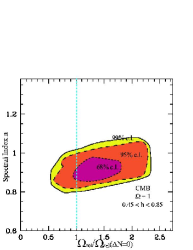
We have analyzed this in [25]. In Figure 9 we plot the likelihood contours for $\omega_{rel}$ vs $\omega_{m},\omega_{b}$ and $n_{s}$ (left to right). As we can see, $\omega_{rel}$ is weakly constrained to be in the range $1\leq\omega_{rel}/\omega_{rel}(\Delta N_{\nu}=0)\leq 1.9$ at $1-\sigma$ in all the plots. The degeneracy between $\omega_{rel}$ and $\omega_{m}$ is evident in the left panel of Figure 9. Increasing $\omega_{rel}$ shifts the epoch of equality and this can be compensated only by a corresponding increase in $\omega_{m}$. It is interesting to note that even if we are restricting our analysis to flat models, the degeneracy is still there and that the bounds on $\omega_{m}$ are strongly affected. We find $\omega_{m}=0.2\pm 0.1$, to be compared with $\omega_{m}=0.13\pm 0.04$ when $\Delta N_{\nu}$ is kept to zero. It is important to realize that these bounds on $\omega_{rel}$ appear because of our prior on $h$ and because we consider flat models. When one allows $h$ as a free parameter and any value for $\Omega_{m}$, then the degeneracy is almost complete. In principle, a critical univers with $\Omega_{M}=1$ could be put back in agreement with CMB and LSS observations by this mechanism ([95]). In the center and right panel of Fig.9 we plot the likelihood contours for $\omega_{b}$ and $n_{s}$. As we can see, these parameters are not strongly affected by the inclusion of $\omega_{rel}$ and the most relevant degeneracy is with the amount of non relativistic matter $\omega_{m}$. An accurate determination of $\omega_{cdm}=\omega_{m}-\omega_{b}$ can shed new light on the nature of dark matter. The thermally averaged cross-sections times velocity of the dark matter candidate is related to $\omega_{cdm}$, and this relation is currently used to analyze the implications for the mass spectra in versions of the Supersymmetric Standard Model (see e.g. [8], [37], [55]).

5.5 Varying $\alpha$

Figure 10: BBN and CMB likelihood contours for variations in the fine structure constant $\alpha$. Picture taken from [5]

There are quite a large number of experimental constraints on the value of fine structure constant $\alpha$. These measurements cover a wide range of timescales (see [132] for a review of this subject), starting from present-day laboratories ($z\sim 0$), geophysical tests ($z<<1$), and quasars ($z\sim 1\div 3$), through the CMB ($z\sim 10^{3}$) and BBN ($z\sim 10^{10}$) bounds.

The recent analysis of [108] of fine splitting of quasar doublet absorption lines gives a $4\sigma$ evidence for a time variation of $\alpha$, $\Delta\alpha/\alpha=(-0.72{\pm}0.18)10^{-5}$, for the redshift range $z\sim 0.5-3.5$. This positive result was obtained using a many-multiplet method, which, it is claimed, achieves an order of magnitude greater precision than the alkali doublet method. Some of the initial ambiguities of the method have been tackled by the authors with an improved technique, in which a range of ions is considered, with varying dependence on $\alpha$, which helps reduce possible problems such as varying isotope ratios, calibration errors and possible Doppler shifts between different populations of ions [109, 30, 136, 110].

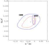
The present analysis of the $\alpha$-dependence of two relevant cosmological observables like the anisotropy of CMB and the light element primordial abundances does not support evidence for variations of the fine-structure constant at more than the one-sigma level at either epoch. The $68\%$ and $95\%$ C.L. regions in the plane $\Omega_{b}h^{2}$– $\Delta\alpha/\alpha$ are shown in Fig. 10 from CMB and BBN (see [5] and references therein).

5.6 Isocurvature modes.

Another key assumption is that the primordial fluctuations were adiabatic. Adiabaticity is not a necessary consequence of inflation though and many inflationary models have been constructed where isocurvature perturbations would have generically been concomitantly produced (see e.g. [92], [64], [10]).

In a phenomenological approach one should consider the most general primordial perturbation, introduced by [28], and described by a $5X5$ symmetric matrix-valued generalization of the power spectrum. As showed by [28], the inclusion of isocurvature perturbations with auto and cross-correlations modes has dramatic effects on standard parameter estimation with uncertainties becoming of order one.

Even assuming priors such as flatness, the inclusion of isocurvature modes significantly enlarges our constraints on the baryon density [130] and the scalar spectral index [4]. Pure isocurvature perturbations are highly excluded by present CMB data ([56]).

As we saw in the first section, it is also possible to have active and decoherent perturbations such as those produced by an inhomogeneously distributed form of matter like topological defects. Models based on global defects like cosmic strings and textures are excluded at high significance by the present data (see e.g. [47]). However a mixture of adiabatic$+$defects is still compatible with the observations ([24], [47]). In principle, toy models based on active perturbations can be constructed [131] that can mimic inflation and retain a good agreement with observations [48].

6 Conclusions

The recent CMB data represent a beautiful success for the standard cosmological model. The acoustic oscillations in the CMB angular power spectrum, a major prediction of the model, have now been detected at $\sim 5\sigma$ C.L. for the first peak and $\sim 2\sigma$ C.L. for the second and third peak. Furthermore, when constraints on cosmological parameters are derived under the assumption of adiabatic primordial perturbations the following results are obtained:

• The curvature of the universe is zero, i.e. the universe is flat, in agreement with the predictions of the theory.

• The power spectrum of the primordial perturbations is nearly scale-invariant, again a prediction of the model.

• The amount of density in baryons is in agreement with independent observations of primordial abundances and standard big-bang nucleosynthesis.

• The optical depth is constrained to be $\tau_{c}<0.3$, and the universe recombined, in agreement with the overall scenario.

• Some form of non baryonic dark matter must be present, as requested by a large set of independent observations.

• The age of the universe is consistent with at least $3$ independent constraints.

• When information from complementary datasets, like constraint on $h$ or from large scale structure, are included in the analysis, the CMB data suggest a presence for a cosmological constant in agreement with the SN-Ia result.

All these results strongly suggest that the inflationary scenario of structure formation is coherent in its simplest form. In few words, the hoped-for miracle.

As we saw in the previous section, modifications to this model, like adding isocurvature modes or topological defects, are in agreement with the observations, but are not required by the data and are reasonably constrained when complementary datasets are included in the analysis.

Since the model is in agreement with the data and all the most relevant parameters are starting to be constrained within a few percent accuracy, the CMB is becoming a wonderful laboratory for investigating the possibilities of new physics. With the promise of large data sets from Map, Planck and SNAP satellites, opportunities may be open, for example, to constrain dark energy models, variations in fundamental constants and neutrino physics.

ACKNOWLEDGEMENTS

First of all, I wish to thank all the organizers of this exciting conference: Matts Roos, Kari Enqvist, Hannu Kurki-Suonio, Anna Kalliomaki Antti Sorri and Jussi Valiviita in particular. I am grateful to Becky Bowen and Steen Harle Hansen for comments and suggestions. Many thanks also to Rachel Bean, Celine Boehm, Sarah Bridle, Rob Crittenden, Ruth Durrer, Pedro Ferreira, Ignacio Ferreras, Will Kinney, Gianpiero Mangano, Carlos Martins, Gennaro Miele, Marco Peloso, Ofelia Pisanti, Antonio Riotto, Graca Rocha, Joe Silk, and Roberto Trotta for comments, discussions and help.

References

- [1] I. Affleck and M. Dine, Nucl. Phys. B249 (1985) 361.
- [2] A. Albrecht, D. Coulson, P.G. Ferreira and J. Magueijo, Phys. Rev. Lett. 76, 1413 (1996).
- [3] B. Allen et al., Phys. Rev. Lett. 79, 2624 (1997).
- [4] L. Amendola, C. Gordon, D. Wands and M. Sasaki, arXiv:astro-ph/0107089.
- [5] P. P. Avelino et al., Phys. Rev. D 64, 103505 (2001) [arXiv:astro-ph/0102144].
- [6] A. Balbi et al., Astrophys. J. 545 (2000) L1 [Erratum-ibid. 558 (2000) L145] [arXiv:astro-ph/0005124].
- [7] J.M Bardeen, Phys. Rev. D22 1882–1905, 1980.
- [8] V. Barger, C. Kao, hep-ph/0106189
- [9] J. Barriga, E. Gaztanaga, M. G. Santos and S. Sarkar, Mon. Not. Roy. Astron. Soc. 324 (2001) 977 [arXiv:astro-ph/0011398].
- [10] N. Bartolo, S. Matarrese and A. Riotto, Phys. Rev. D 64 (2001) 123504 [arXiv:astro-ph/0107502].
- [11] R. Bean, S. H. Hansen and A. Melchiorri, Phys. Rev. D 64 (2001) 103508 [arXiv:astro-ph/0104162].
- [12] R. Bean and A. Melchiorri, arXiv:astro-ph/0110472, Phys. Rev. D Rapid Communication, in press.
- [13] G. Beaudet and P. Goret, Astron. & Astrophys. 49 (1976) 415.
- [14] P. de Bernardis, A. Balbi, G. De Gasperis, A. Melchiorri and N. Vittorio, arXiv:astro-ph/9609154.
- [15] P. de Bernardis et al. [Boomerang Collaboration] astro-ph/9911461.
- [16] P. de Bernardis et al. [Boomerang Collaboration], Nature 404, 955 (2000) [arXiv:astro-ph/0004404].
- [17] P. de Bernardis et al., [Boomerang Collaboration], arXiv:astro-ph/0105296.
- [18] S. A. Bludman and M. Roos, arXiv:astro-ph/0109551.
- [19] C. Boehm, A. Melchiorri, M. Peloso, in preparation (2002).
- [20] J. R. Bond, Class. Quant. Grav. 15 (1998) 2573.
- [21] J. R. Bond et al. [The MaxiBoom Collaboration], astro-ph/0011379.
- [22] J. R. Bond and G. Efstathiou, Astrophys. J. 285 (1984) L45.
- [23] J. Borrill, proceedings of ‘3K Cosmology Euroconference’, Roma, ed F. Melchiorri, astro-ph/9903204.
- [24] F. R. Bouchet, P. Peter, A. Riazuelo and M. Sakellariadou, Phys. Rev. D 65 (2002) 021301 [arXiv:astro-ph/0005022].
- [25] R. Bowen et al., arXiv:astro-ph/0110636.
- [26] P. Brax, J. Martin & A. Riazuelo, Phys. Rev. D.,62 103505 (2000).
- [27] S. L. Bridle, R. Crittenden, A. Melchiorri, M. P. Hobson, R. Kneissl and A. N. Lasenby, arXiv:astro-ph/0112114.
- [28] M. Bucher, K. Moodley and N. Turok, Phys. Rev. D 62 (2000) 083508 [arXiv:astro-ph/9904231].
- [29] S. Burles, K. M. Nollett and M. S. Turner, Astrophys. J. 552, L1 (2001) [arXiv:astro-ph/0010171].
- [30] C.L. Carilli et al., Phys. Rev. Lett. 85, 5511 (2001).
- [31] A. Casas, W.Y. Cheng, and G. Gelmini, Nucl. Phys. B538 (1999) 297.
- [32] R. Cayrel et al., Nature 409, 691–692 (2001)
- [33] E. J. Copeland, I. J. Grivell and A. R. Liddle, arXiv:astro-ph/9712028.
- [34] L. Covi and D. H. Lyth, arXiv:astro-ph/0008165.
- [35] R. Crittenden, J. R. Bond, R. L. Davis, G. Efstathiou and P. J. Steinhardt, Phys. Rev. Lett. 71 (1993) 324[arXiv:astro-ph/9303014].
- [36] P. Di Bari and R. Foot, Phys. Rev. D63 (2001) 043008.
- [37] A. Djouadi, M. Drees, J.L. Kneur, hep-ph/0107316
- [38] S. Dodelson and E. Stewart, arXiv:astro-ph/0109354.
- [39] A.D. Dolgov and D.P. Kirilova, J. Moscow Phys. Soc. 1 (1991) 217.
- [40] A.D. Dolgov, Phys. Rep.222 (1992) 309.
- [41] A.G. Doroshkevich, I.D. Novikov, R.A. Sunaiev, Y.B. Zeldovich, in Highlights of Astronomy, de Jager ed., (1971) p. 318.
- [42] M. Douspis, A. Blanchard, R. Sadat, J.G. Bartlett, M. Le Dour, Astronomy and Astrophysics, v.379, p.1-7 (2001).
- [43] M. Douspis & P. Ferreira, astro-ph/0111400, (2001).
- [44] R. Durrer, Phys. Rev. D42 2533-2541 (1990).
- [45] R. Durrer, arXiv:astro-ph/0109522.
- [46] R. Durrer, M. Kunz and A. Melchiorri, Phys. Rev. D 59 123005 (1999).
- [47] R. Durrer, M. Kunz and A. Melchiorri, arXiv:astro-ph/0110348.
- [48] R. Durrer, M. Kunz and A. Melchiorri, Phys. Rev. D 63 (2001) 081301 [arXiv:astro-ph/0010633].
- [49] R. Durrer, B. Novosyadlyj, S. Apunevych, astro-ph/0111594.
- [50] R. Durrer and M. Sakellariadou, Phys. Rev. D 56, 4480 (1997).
- [51] S. Dodelson and L. Knox, Phys. Rev. Lett. 84, 3523 (2000) [arXiv:astro-ph/9909454].
- [52] G. Efstathiou, astro-ph/0109151.
- [53] G. Efstathiou & J.R. Bond [astro-ph/9807103].
- [54] O. Elgaroy, M. Gramann, O. Lahav [astro-ph/0111208].
- [55] J. R. Ellis, D. V. Nanopoulos, & K. A. Olive, 2001, Phys. Lett. B 508 65
- [56] K. Enqvist, H. Kurki-Suonio and J. Valiviita, arXiv:astro-ph/0108422.
- [57] S. Esposito, G. Mangano, A. Melchiorri, G. Miele, and O. Pisanti, Phys. Rev. D63 (2001) 043004.
- [58] P. Ferreira and M. Joyce, Phys.Rev. D58 (1998) 023503.
- [59] I. Ferreras, A. Melchiorri and J. Silk, MNRAS 327, L47 (2001), arXiv:astro-ph/0105384.
- [60] R.Foot, M.J.Thomson and R.R.Volkas, Phys. Rev. D53 (1996) 5349.
- [61] W.A. Fowler, Accademia Nazionale dei Lincei, Roma 157 (1971) 115.
- [62] W. Freedman et al., Astrophysical Journal, 553, 2001, 47.
- [63] P.M. Garnavich et al, Ap.J. Letters 493, L53-57 (1998); S. Perlmutter et al, Ap. J. 483, 565 (1997); S. Perlmutter et al (The Supernova Cosmology Project), Nature 391 51 (1998); A.G. Riess et al, Ap. J. 116, 1009 (1998); B.P. Schmidt, Ap. J. 507, 46-63 (1998).
- [64] C. Gordon, D. Wands, B. A. Bassett and R. Maartens, Phys. Rev. D 63 (2001) 023506 [arXiv:astro-ph/0009131].
- [65] L. M. Griffiths, A. Melchiorri and J. Silk, Astrophys. J. 553 (2001) L5 [arXiv:astro-ph/0101413].
- [66] L. M. Griffiths et al., astro-ph/0010571.
- [67] Z. Haiman and L. Knox, arXiv:astro-ph/9902311.
- [68] N. W. Halverson et al., arXiv:astro-ph/0104489.
- [69] S. Hanany et al., Astrophys. J. 545, L5 (2000) [arXiv:astro-ph/0005123].
- [70] S. Hannestad, Phys. Rev. Lett. 85 (2000) 4203 [arXiv:astro-ph/0005018].
- [71] S. Hannestad, Phys. Rev. D 64 (2001) 083002 [arXiv:astro-ph/0105220].
- [72] S. Hannestad, S. H. Hansen and F. L. Villante, Astropart. Phys. 16 (2001) 137 [arXiv:astro-ph/0012009].
- [73] S. Hannestad, S. H. Hansen, F. L. Villante and A. J. Hamilton, arXiv:astro-ph/0103047.
- [74] S.H. Hansen and F.L. Villante, Phys. Lett. B486 (2000) 1.
- [75] S. H. Hansen, G. Mangano, A. Melchiorri, G. Miele and O. Pisanti, Phys. Rev. D 65 (2002) 023511 [arXiv:astro-ph/0105385].
- [76] E. Hivon, K.M. Gorski, C.B. Netterfield, B.P. Crill, S. Prunet, F. Hansen, astro-ph/0105302.
- [77] M. B. Hoffman, M. S. Turner, Phys.Rev. D64 (2001) 023506, astro-ph/0006312.
- [78] W. Hu, astro-ph/9801234.
- [79] W. Hu, D. Scott, N. Sugiyama and M. J. White, Phys. Rev. D 52, 5498 (1995) [arXiv:astro-ph/9505043].
- [80] W. Hu, N. Sugiyama and J. Silk, Nature 386, 37 (1997) [arXiv:astro-ph/9604166].
- [81] A.H. Jaffe et al., Phys. Rev. Lett., 86 (2001) 3475.
- [82] H. Kang and G. Steigman, Nucl. Phys. B372 (1992) 494.
- [83] M. Kaplinghat and M.S. Turner, Phys. Rev. Lett. 86 (2001) 385.
- [84] W. H. Kinney, A. Melchiorri and A. Riotto, Phys. Rev. D 63 (2001) 023505[arXiv:astro-ph/0007375].
- [85] J. P. Kneller, R. J. Scherrer, G. Steigman and T. P. Walker, Phys. Rev. D 64 (2001) 123506 [arXiv:astro-ph/0101386].
- [86] L. Knox, Phys. Rev. D 52, 4307 (1995) [arXiv:astro-ph/9504054].
- [87] L. Knox, N. Christensen, C. Skordis, [arXiv:astro-ph/0109232].
- [88] L. Knox and L. Page, Phys. Rev. Lett. 85, 1366 (2000) [arXiv:astro-ph/0002162].
- [89] A. Kosowsky and M. S. Turner, Phys. Rev. D 52 (1995) 1739 [arXiv:astro-ph/9504071].
- [90] O. Lay and N. Halverson, Astrophys. J., 543, 787, (2000).
- [91] A. E. Lange et al. [Boomerang Collaboration], Phys. Rev. D 63 (2001) 042001 [arXiv:astro-ph/0005004].
- [92] D. Langlois and A. Riazuelo, Phys. Rev. D 62 (2000) 043504.
- [93] A. T. Lee et al., Astrophys. J. 561 (2001) L1 [arXiv:astro-ph/0104459].
- [94] E. M. Leitch et al., arXiv:astro-ph/0104488.
- [95] J. Lesgourgues and A. R. Liddle, Mon. Not. Roy. Astron. Soc. 327 (2001) 1307 [arXiv:astro-ph/0105361].
- [96] J. Lesgourgues and M. Peloso, Phys. Rev. D 62 (2000) 081301 [arXiv:astro-ph/0004412].
- [97] E. Lisi, S. Sarkar, and F.L. Villante, Phys. Rev. D59 (1999) 123520.
- [98] D. H. Lyth and L. Covi, Phys. Rev. D 62 (2000) 103504 [arXiv:astro-ph/0002397].
- [99] J. March-Russell, H. Murayama, and A. Riotto, JHEP 11 (1999) 015.
- [100] P. D. Mauskopf et al. [Boomerang Collaboration], Astrophys. J. 536, L59 (2000) [arXiv:astro-ph/9911444].
- [101] J.McDonald, Phys. Rev. Lett. 84 (2000) 4798.
- [102] S. S. McGaugh, Astrophys. J. 541 (2000) L33 [arXiv:astro-ph/0008188].
- [103] A. Melchiorri and L. M. Griffiths, arXiv:astro-ph/0011147.
- [104] A. Melchiorri et al. [Boomerang Collaboration], Astrophys. J. 536 (2000) L63 [arXiv:astro-ph/9911445].
- [105] A. Melchiorri, M. V. Sazhin, V. V. Shulga and N. Vittorio, Astrophys. J. 518 (1999) 562[arXiv:astro-ph/9901220].
- [106] A. Melchiorri and N. Vittorio, arXiv:astro-ph/9610029.
- [107] A. D. Miller et al., Astrophys. J. 524, L1 (1999) [arXiv:astro-ph/9906421].
- [108] M.T. Murphy, J.K. Webb, V.V. Flambaum, V.A. Dzuba, C.W. Churchill, J.X. Prochaska, J.D. Barrow, and A.M. Wolfe, astro-ph/0012419.
- [109] M.T. Murphy, J.K. Webb, V.V. Flambaum, J.X. Prochaska, and A.M. Wolfe, astro-ph/0012421.
- [110] M.T. Murphy, J.K. Webb, V.V. Flambaum, M.J. Drinkwater, F. Combes, and T. Wiklind, astro-ph/0101519.
- [111] C. B. Netterfield et al. [Boomerang Collaboration], arXiv:astro-ph/0104460.
- [112] M. Orito, T. Kajino, G. J. Mathews and R. N. Boyd, arXiv:astro-ph/0005446.
- [113] P.J.E. Peebles, and Yu, J.T. 1970, Ap.J. 162, 815
- [114] U. Pen, U. Seljak and N. Turok, Phys. Rev. Lett. 79, 1611 (1997).
- [115] S. Perlmutter, M.S. Turner, M. White, Phys.Rev.Lett. 83 670-673 (1999).
- [116] F. Piacentini et al, astro-ph/0105148 (2002).
- [117] C. Pryke, N. W. Halverson, E. M. Leitch, J. Kovac, J. E. Carlstrom, W. L. Holzapfel and M. Dragovan, arXiv:astro-ph/0104490.
- [118] S. Prunet et al, astro-ph/0101073.
- [119] G. Rocha & S. Hancock, astro-ph/9611228, proceedings of the XXXIst Rencontre de Moriond, ‘Microwave Background Anisotropies’.
- [120] M. Salaris, & A. Weiss, Astron. Astrophys. 335, 943–953 (1998)
- [121] D. Scott, J. Silk and M. J. White, Science 268, 829 (1995) [arXiv:astro-ph/9505015].
- [122] R. Stompor et al., Astrophys. J. 561 (2001) L7 [arXiv:astro-ph/0105062].
- [123] R. Stompor et al., Phys. Rev. D 65 (2002) 022003.
- [124] Sunyaev, R.A. & Zeldovich, Ya.B., 1970, Astrophysics and Space Science 7, 3
- [125] M. Tegmark, Astrophys. J. 514, L69 (1999) [arXiv:astro-ph/9809201].
- [126] M. Tegmark, G, Efstathiou, astro-ph/9507009, MNRAS, 281, 1297-1314, 1995.
- [127] M. Tegmark, D. J. Eisenstein, W. Hu and A. de Oliveira-Costa, Astrophys. J. 530 (2000) 133 [arXiv:astro-ph/9905257].
- [128] M. Tegmark and M. Zaldarriaga, Phys. Rev. Lett. 85 (2000) 2240.
- [129] E. Torbet et al., Astrophys. J. 521, L79 (1999) [arXiv:astro-ph/9905100].
- [130] R. Trotta, A. Riazuelo and R. Durrer, Phys. Rev. Lett. 87 (2001) 231301.
- [131] N. Turok, Phys. Rev. Lett. 77 (1996) 4138 [arXiv:astro-ph/9607109].
- [132] D.A. Varshalovich, A.Y. Potekhin, and A.V. Ivanchik, physics/0004062.
- [133] N. Vittorio, J. Silk, ApJ, 285L,39 (1984).
- [134] Y. Wang and G. Mathews, arXiv:astro-ph/0011351.
- [135] X. Wang, M. Tegmark, M. Zaldarriaga, astro-ph/0105091.
- [136] J.K. Webb, M.T. Murphy, V.V. Flambaum, V.A. Dzuba, C.W. Churchill, J.X. Prochaska, J.D. Barrow, and A.M. Wolfe, astro-ph/0012539.
- [137] J. Weller, A. Albrecht, Phys.Rev.Lett. 86 1939 (2001) [astro-ph/0008314]; D. Huterer and M. S. Turner, [astro-ph/0012510]; M. Tegmark, [astro-ph/0101354].
- [138] C. Wetterich, Nucl. Phys B. 302 668 (1988)
- [139] M. J. White, D. Scott and J. Silk, Ann. Rev. Astron. Astrophys. 32 (1994) 319.
- [140] M. L. Wilson and J. Silk, Astrophys. J. 243 (1981) 14.
- [141] M. Yahiro, G. J. Mathews, K. Ichiki, T. Kajino and M. Orito, arXiv:astro-ph/0106349.
- [142] I. Zlatev, L. Wang, & P. Steinhardt, Phys. Rev. Lett. 82 896-899 (1999).