A New Upper Limit on the Large Angular Scale Polarization of the Cosmic Microwave Background Radiation

2001

Peter Timbie Professor

Abstract

The Cosmic Microwave Background Radiation (CMB) is an invaluable probe of the conditions of the early universe. Recent measurements of its spatial anisotropy have allowed accurate determinations of several fundamental cosmological parameters, such as the curvature of the universe, the shape of the spectrum of primordial density fluctuations, and the contribution of baryons, dark matter, and dark energy to the overall energy density of the universe. In addition to being spatially non-uniform, the CMB is theorized to be slightly polarized. Measurements of this polarization, particularly at large angular scales, have the potential to provide information on primordial gravitational waves, theories of inflation, and the ionization history of the universe, as well as help further constrain cosmological parameters.

Polarization has not yet been detected in the CMB. This thesis describes a recent search for CMB polarization at large angular scales, conducted in the spring of 2000 at the University of Wisconsin-Madison. After a general introduction on both CMB polarization and general microwave polarimetry, details of the experiment itself are given, as well as a full description of the data selection and analysis techniques. Using these techniques, our data lead to a new upper limit on CMB polarization at large angular scales of 10 $\mu$K in both E- and B-type polarization at 95% confidence. If B-polarization is assumed to be zero, the limit for E-type polarization is lowered to 8 $\mu K$. This experiment is the first of a new breed of highly-sensitive instruments that will one day map out this interesting property of the Cosmic Microwave Background radiation.

There are so many people who have given me their time and patience throughout my years in grad school that I would like to thank. First and foremost, I want to thank my advisor, mentor, and friend Peter Timbie, who has been a truly wonderful thesis advisor. Peter always showed patience with me while I explained the newest problem in my thesis; he had a knack of being able to get to the root of any problem, for which I was grateful on several occasions. He also gave me great freedom as a graduate student and allowed me to make my own mistakes, and has helped me to truly grow as a scientist.

Someone who taught me immeasurable quantities of radiometric knowledge, Brian Keating, also deserves much credit. Thanks to him I have finally memorized the radiometer equation. Brian, if I could have a number of “Meatloaf Carver Combos” equal to the logarithm of what you taught me, I would never go hungry.

I would also like to thank all my science “elders”, who have helped me with so many of the knotty problems that have come up over the years: Dan Mccammon, Don Cox, Josh Gundersen, Bob Benjamin, Ed Wollack, and Grant Wilson. Also, thanks to Max Tegmark and Angelica de Oliveira-Costa, who provided excellent theory mentorship for the data analysis segment of my thesis, and who have been great friends. Thanks to Craig Marquardt, David Fanning, and the rest of the IDL newsgroup who helped with all my IDL issues. Special thanks to Gail Bayler and Gary Wade at the UW Space Sciences and Engineering center who provided all the wonderful GOES satellite data for use in this project.

Thanks to all the technicians and machine-shop “artists” I have had the privilege to work with: Walt Wigglesworth, who taught me everything I know about machining; Lee Potratz and the entire Instrument shop team, who constructed so many of the critical elements that POLAR utilized; and finally all the guys in the Stirling Hall electronics shop, who built me so many power supplies that I could have probably separated every hydrogen atom on Earth.

A big “shout-out” to all the people I had the honor of knowing and working with over the years in the Wisconsin Observational Cosmology Lab. Slade Klawikowski, who was a great partner in the construction and running of POLAR, and was much better than I at keeping POLAR warm and dry; Karen Lewis, the best cookie tzarina this side of the Mississippi; the “wonder twins” Jodi and Mark Supanich, Nate Stebor, Dan “Crowbar” Swetz, Zak Staniszewski, Kip Hyatt, Marye “Molly” Reed, and Josh “H to the izz-O” Friess. Not only were you all great to work with, you all made the lab fun, a place I actually wanted to be!

Finally, I want to recognize my friends, who over the years have truly been my family and without whom I don’t know where I’d be. It’s hard to name you all, but you know who you are. Jack and Karyn, you always reminded me the right way to live, that you have to pull your head out of the details and smell the roses every once in a while. Melanie Barker, who has been my support and good friend so long; thanks for giving me so much over the years. I think I still owe you many hundreds of Meow-Meow bucks. John Wright, the best roommate and biking partner and Latex mentor a guy could ever ask for. Rob Haslinger, who was always willing to go out for a beer, who always wanted to live it up in Madison and was a great partner-in-crime on so many occasions. Bruce and Oleg, Jay and Ted, Lisa J, Jen and Stefan, Christine and Steve and the rest of the “Jeffer-Gang”; it was great enjoying Wisconsin with you. And of course, my entire Dayton family, the “Platt”, who I miss dearly and who always provided me with a fantastic home-away-from-home: Jeff, Trevor, Randy, Christine, Curt, Alicia and Joe and Michael and Marie, Mike Collins, Chris Corn, and all the rest of the Daytonites. The times I went home and visited with you were my times of spiritual healing.

Dedication

This thesis is dedicated to my parents, who put so much of themselves into me that this work is as much a reflection of their hard work as parents as it is mine as a student.

To my father, who first introduced me to the beauty and wonder of physics; when he gave me his well-loved copy of One, Two, Three..Infinity; when he climbed our tv-antenna fifty feet in the air, in what were surely hurricane-force winds, to help me with my first science project; and when he suffered all my frustrations with patience and love. Dad, you have truly made me what I am today.

To my mother, who has always put her children before herself, I can’t imagine what life would have been like without you. From sitting in the kitchen helping me with vocabulary, to all your little lessons on life, I owe a large debt of love to you.

This thesis is also dedicated to Jeff Hessell, who taught me and gave me so much during my life, who showed me the beauty and enormity of the night sky. From using your telescope to see the moons of Jupiter and the rings of Saturn, to wondering how the universe began, those times we spent on the roof gazing upward at the heavens have never really stopped.

Chapter 1 Introduction

1.1 The Pillars of Cosmology

The understanding of the origin of the universe has greatly evolved over the course of human history. We initially believed a multitude of religion-based creation theories. During the last century, however, these beliefs were largely superseded by scientifically-based theories, from a steady-state picture of a static universe, as was popular in the early part of the 20th century, to the current Hot Big Bang model of modern cosmology. The Big Bang Model rests upon three sturdy “pillars” of observational evidence. In 1929, Edwin Hubble discovered that virtually every galaxy he observed was moving away from us, and the galaxies’ recessional velocities were roughly proportional to their distances from us. This led to the famous “Hubble Law” of the expansion of the universe, measurements of which have greatly improved over the last seventy years (see Figure 1.1). Today, the Hubble constant is known with unprecedented accuracy, and similar observations have led to a measurement of the deceleration parameter and the conclusion that the expansion appears to be accelerating [1, 2, 3].

Figure 1.1: Modern Measurements of Hubble’s Law. Plotted is the apparent magnitude minus absolute magnitude (which is proportional to the logarithm of distance) versus redshift, along with three cosmological models. In addition to illustrating Hubble’s Law, this work is accurate enough to determine the rate of change of Hubble’s constant, and is consistent with an accelerating universe. Adopted from [3].

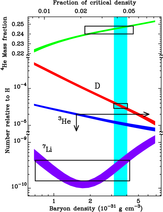
The discovery of galaxy redshifts in and of itself led to the idea of a universe in which space itself is expanding, and necessarily requires that the universe was much smaller, hotter and denser in the past. Running from the beginning of the universe forward, there would therefore be a time when the universe cooled enough to create nuclei from free protons and neutrons, themselves in a virtual “soup” of particles with electrons, photons, and other less abundant species. This era of “Big Bang Nucleosynthesis” (BBN) is entirely calculable, and can predict elemental abundances of the light nuclei. These predictions closely match current observations, and have led to a measurement of the primordial entropy of the universe, expressed in the baryon-to-photon ratio (see Figure 1.2). To date, the match between observations and theory is remarkable [4, 5].

Figure 1.2: Predictions of BBN for the four most important light elements versus the baryon density in the universe (this is an equivalent alternative to the baryon-to-photon ratio, $\eta$, sometimes used, as well as $\Omega_{b}h^{2}$). The boxes show the 95% confidence limits of observations of primordial abundances. There is really only one acceptable value for the baryon density, and that is $\Omega_{b}h^{2}=0.020\pm 0.002$ (95% confidence) [5]. Figure adopted from [4].

The final observational pillar of the Big Bang is the Cosmic Microwave Background radiation (CMB), discovered in 1965 by Arno Penzias and Robert Wilson of Bell Telephone Laboratories [6]. If the Big Bang actually happened, this background of microwaves necessarily exists. Its existence was first postulated by George Gamow and his students in 1948 [7], and the theory describing the CMB was later refined by others, notably Robert Dicke and James Peebles of Princeton [8].

1.2 Origin and Characteristics of the CMB

During the first 100,000 years, the universe was completely ionized, its primary matter components being free protons and electrons. When the universe had cooled to a temperature of about 3000 Kelvin, it was cold enough for electrons and protons to stick together as hydrogen atoms, without an energetic photon immediately reionizing them. This was the beginning of the era of “recombination” during which the universe rapidly went from ionized to neutral, and led to the release of CMB photons. This can be thought of as happening on a “surface in redshift space”, which is commonly called the last scattering surface (LSS).

1.2.1 Spectrum

Because the universe had undergone a period of thermal equilibrium in its history, the CMB was initially created with a blackbody spectrum. It can be shown that a blackbody radiation field in an expanding universe retains its blackbody spectrum, but its characteristic temperature decreases in proportion to the scale factor of the universe [9]. The spectrum of the CMB was measured by the FIRAS (Far-Infrared Absolute Spectrophotometer) instrument aboard the COBE (Cosmic Background Explorer) COBE satellite in 1989, during its very first days in space. As shown in Figure 1.3, it was consistent with a perfect blackbody; in fact, the FIRAS measurement is the most perfect measurement of a blackbody ever performed. It corresponds to a temperature of 2.7253 $K$ $\pm$ 0.66 $mK$ [10].

Figure 1.3: Measurements of the CMB spectrum. The most constraining measurements come from the FIRAS instrument aboard COBE [11], although the spectrum has since been measured at a variety of frequencies well away from the blackbody peak. Adopted from [12].

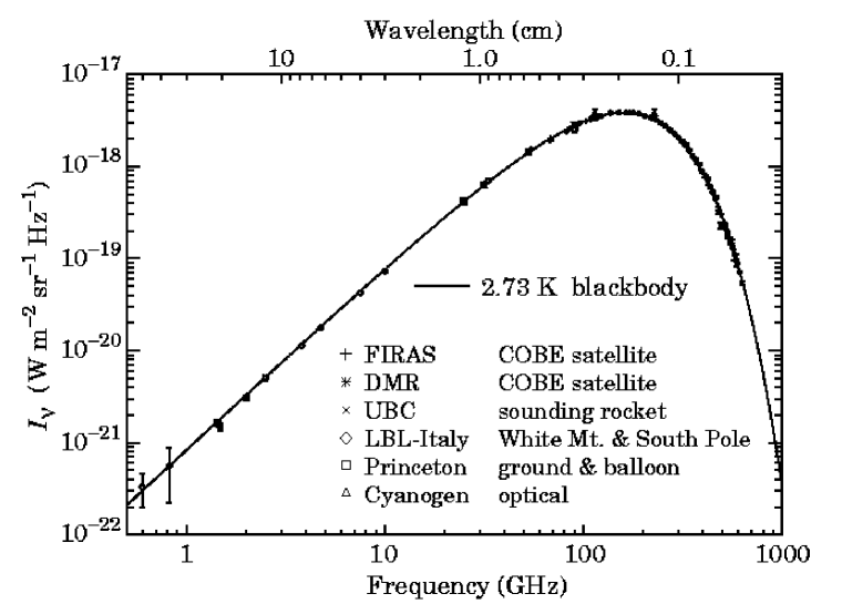
Deviations from a blackbody are expected at low levels due to various forms of “energy injections” into the universe at times during and since recombination. Energy released via starlight would heat up whatever free electrons there were, and these (now hotter) electrons would transfer some energy to the CMB via Compton scattering. This would cause the CMB spectrum to be an admixture of different blackbody curves, causing a distortion in the spectrum due to a decrement of photons at lower energies and and increment of photons at higher energies. This distortion is characterized by the Compton $y$-parameter, defined by $y=\int k_{B}(T_{e}-T_{cmb})/m_{e}c^{2}d\tau$, where $T_{e}$ is the kinetic temperature of the electrons and $\tau$ is the optical depth of free electrons to last scattering. The best upper limits on $y$ are from COBE, and suggest $|y|<15\times 10^{-6}$ [13]. A proposed satellite mission may further illuminate the history of spectrum-distorting mechanisms in the universe [14].

1.2.2 Spatial Anisotropy

The CMB is not uniform in its intensity on the sky, but rather varies from place to place. The primary anisotropy in the CMB is due to the Earth’s relative motion with respect to the rest frame of the CMB; this leads to the so-called “dipole anisotropy”, which is a temperature difference of 3.353 $\pm$ 0.024 mK in the CMB sky (corresponding to an Earth velocity of about 370 km/sec with respect to this “cosmic rest frame”) [13].

Initial seeds of structure, present in the early universe in the form of perturbations to the Robertson-Walker metric, imprinted themselves upon the CMB during last scattering. They are imprinted on the CMB primarily via the Sachs-Wolfe mechanism [15], in which CMB photons originating from an overdense region are forced to climb out of the local gravitational well; therefore, areas of the sky with less CMB intensity than average correspond to overdense regions, and likewise increased CMB intensity corresponds to underdense regions. There are other effects that couple density perturbations to the CMB; for an excellent introduction to these processes, see [16].

If the fluctuations in the microwave background intensity are a Gaussian random variable, then all the information in anisotropy is included in the two-point autocorrelation function, $C(\theta)$, of the fluctuations [17]:

$$C(\theta)\equiv\langle\frac{\Delta T({\bf x})}{T_{cmb}}\frac{\Delta T({\bf x}^{\prime})}{T_{cmb}}\rangle$$ (1.1)

where $\Delta T({\bf x})/T_{cmb}$ is the fractional deviation in the CMB temperature in the direction ${\bf x}$, and the average is over all pairs of directions on the sky ${\bf x}$ and ${\bf x}^{\prime}$ such that ${\bf x}\cdot{\bf x}^{\prime}=\cos{\theta}$. This function $C(\theta)$ then contains all the information contained in the anisotropy, and can be expanded in terms of Legendre polynomials, where the information is in turn kept in the $C_{\ell}$ coefficients:

$$C(\theta)\ =\ \frac{1}{4\pi}\sum_{\ell}C_{\ell}P_{\ell}(\cos{\theta})\ .$$ (1.2)

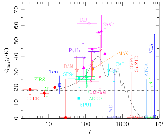
The $C_{\ell}$’s comprise the angular power spectrum of CMB anisotropy. The power spectrum is truly “powerful”; it depends sensitively on the fundamental parameters of cosmology, and by measuring it accurately, over the years we have been able to rule out many theories of structure formation in the universe, and constrain the current theories of cosmology rather tightly. Figure 1.4 shows the state of anisotropy observations, and is a testament to technology, dedication and driving curiosity. The upper panel shows the state of the angular power spectrum as it was just four years ago (when I started working on the CMB), and the lower panel shows the situation today.

Figure 1.4: Anisotropy Power Spectrum Measurements: Old and New. Panel (a) shows the state of power spectrum measurements circa 1997 (adopted from [12]). The quantity shown, $Q_{rms}$ is the angular power spectrum normalized to the COBE measurement of the quadrupole moment. Clearly, the spectrum is not well-constrained, and at one time the error bars on most cosmological parameters were huge or non-existent. Panel (b) shows the situation as of 2001; with measurements by DASI, Maxima-I, and BOOMERANG, the spectrum is reasonably well-sampled out to the second doppler peak at $\ell\approx 600$ (adopted from[18]).

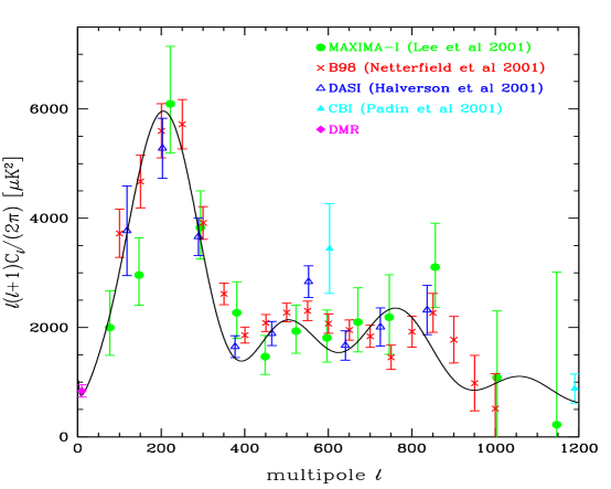
The most recent measurements by the BOOMERANG, MAXIMA-1, and DASI teams have led to an excellent determination of the CMB power spectrum for multipoles less than about 600 [19, 20, 21]. These measurements, along with recent supernova-1a results (such as shown in Figure 1.1), observations of large-scale structure, and measurements of the primordial abundance of light elements have helped not only to confirm the Hot Big Bang paradigm that now dominates cosmology, but also to nail down several of the fundamental parameters that characterize the theory. Indeed, we now have good measurements of many fundamental parameters: the Hubble constant, the age of the universe, the relative content of baryons, dark matter, and dark energy in the universe, the overall curvature of the universe, a strong upper bound on the epoch of reionization, and the spectral index of primordial scalar fluctuations. Table 1.1 shows a compilation of the most recent measurements of these quantities. When I began graduate school six years ago, most of these quantities were known to at best within a factor of two!

Parameter	Value	Measurement(s)	Reference
$H_{0}$	68 $\pm$ 3 $km/sMpc^{-1}$	Multiple Methods Combined	[22]
$T_{universe}$	12.3 $\pm$ 1.6 $Gyr$	CMB+HST-Key	[23]
$\Omega_{tot}$	1.0 $\pm$ 0.06	CMB+HST-Key	[23]
$\Omega_{b}h^{2}$	0.02 $\pm$ 0.002	Deuterium+BBN	[23]
$\Omega_{m}h^{2}$	$0.13^{+.04}_{-.02}$	CMB+BBN+HST-Key	[24]
$\Omega_{\Lambda}$	$0.66^{+.10}_{-.17}$	CMB+HST-Key	[23]
$n_{s}$	$0.93^{+.12}_{-.10}$	CMB+HST-Key	[23]
$\tau$	$<0.17$	CMB+PSCz	[23]
$z_{re}$	$7^{+14}_{-2}$	CMB+PSCz+GP	[23]

Table 1.1: Current constraints on selected cosmological parameters. The techniques used to constrain the data are: CMB anisotropy (see references in text), the IRAS Point-Source Survey (PSCz) [25], Big-Bang Nucleosynthesis calculations [5], deuterium abundance measurements [4], the HST-Key project [26], and the Gunn-Peterson Measurement [27].

1.2.3 Polarization

Though anisotropy studies have been remarkably successful, there is a third characteristic of the CMB that we have not yet discussed: its polarization. In contrast to the spectrum and spatial anisotropy of the CMB, not only has polarization not been well measured, it has never been detected at all! Table 1.2 shows a history of the measurements aimed at detecting CMB polarization and the limits they reached. The first realistic measurements of the polarization of the CMB were undertaken by Lubin and Smoot [28] in the late 1970s; since then limits have improved by about an order of magnitude, and experimentalists are inching ever closer to a detection. In the following sections, I will first review the mathematical description of CMB polarization, and then discuss what can be learned from it.

Name	Frequency [GHz]	Angular Res.	Limit [$\frac{T_{pol}}{T_{cmb}}$]
Penzias and Wilson 1965 [6]	4.0	30∘	0.1
Caderni et al. 1978 [29]	100-600	40∘	$\sim 1\times 10^{-3}$ (65%)
Nanos 1979 [30]	9.3	15∘	$6\times 10^{-4}$ (90%)
Lubin & Smoot 1979 [28]	33	7∘	$3\times 10^{-4}$
Lubin & Smoot 1981 [31]	33	7∘	$1\times 10^{-4}$
Lubin et al. 1983 [32]	33	7∘	$7\times 10^{-5}$
Partridge et al. 1988 [33]	5	18”–160”	$6\times 10^{-5}$
Fomalont et al. 1993 [34]	8.44	10”–80”	$2.6\times 10^{-5}$
Wollack et al. 1993 [35]	26–36	1.4∘	$9\times 10^{-6}$
Netterfield et al. 1995 [36]	26–46	1.05∘	$7\times 10^{-6}$
Partridge et al. 1997 [37]	8.44	30”	$1\times 10^{-5}$
Sironi et al. 1998 [38]	33	30∘	$7\times 10^{-5}$
Subrahmanyan et al. 2000 [39]	8.7	2’	$3.7\times 10^{-6}$
Hedman et al. 2000 [40]	84–100	0.24∘	$3.7\times 10^{-6}$
This Work [41]	26–36	7∘	$2.9\times 10^{-6}$

Table 1.2: Results of searches for CMB polarization. Limits are at 95% confidence unless otherwise noted. Data graciously compiled by Josh Gundersen.

1.3 CMB Polarization - Background and Theory

1.3.1 Review of Polarization Description

Let us briefly review the mathematical description of polarization. An electromagnetic wave can in general be written in terms of its electric field as

$$\vec{E}\ =E_{x}\hat{x}+E_{y}\hat{y}$$ (1.3)

where

$$E_{x} =E_{x_{0}}e^{i(kz-\omega t+\phi_{x})}$$

$$E_{y} =E_{y_{0}}e^{i(kz-\omega t+\phi_{y})}\;\;\text{.}$$

It is implicit that one takes the real part of $\vec{E}$ to obtain the physical field. We can equally well describe this radiation by four scalar quantities, the Stokes parameters which are defined as follows [42]:

$$I =\langle E_{x_{0}}^{2}+E_{y_{0}}^{2}\rangle$$ (1.4a)

$$Q =\langle E_{x_{0}}^{2}-E_{y_{0}}^{2}\rangle$$ (1.4b)

$$U =2\langle E_{x_{0}}E_{y_{0}}\cos(\phi_{x}-\phi_{y})\rangle$$ (1.4c)

$$V =2\langle E_{x_{0}}E_{y_{0}}\sin(\phi_{x}-\phi_{y})\rangle,$$ (1.4d)

where $\langle\ldots\rangle$ denotes a time average. For quasimonochromatic light, each component of Equation (1.4) is understood to be averaged over the entire frequency band.

The Stokes parameters $I$ and $V$ are unchanged under rotations of the $\hat{x}-\hat{y}$ plane, but $Q$ and $U$ are not. If we rotate the $\hat{x}-\hat{y}$ axes through an angle $\theta$, the Stokes parameters change as

$$Q^{\prime}=Q\cos{2\theta}+U\sin{2\theta}$$

$$U^{\prime}=-Q\sin{2\theta}+U\cos{2\theta}$$ (1.5)

The angle $\alpha\equiv\frac{1}{2}\arctan{\frac{U}{Q}}$ transforms to $\alpha-\theta$ under the rotation; hence it defines a constant direction in space, which is interpreted as the axis of polarization. Finally, the magnitude of polarization is typically denoted by

$$P\equiv\sqrt{Q^{2}+U^{2}+V^{2}}\ .$$ (1.6)

For a fully polarized signal, $I=P$. A partially polarized signal is said to have a fractional polarization $\Pi\equiv\frac{P}{I}$.

1.3.2 Why is the CMB polarized?

The CMB is partially polarized via Thomson scattering of CMB photons by free electrons at the last scattering surface [43]. This situation is shown schematically in Figure 1.5. An electron on the last scattering surface viewing an anisotropic distribution will generate a polarized radiation distribution if there is a non-zero quadrupole moment to the anisotropic distribution [44]. Following Kosowsky, the cross-section for Thomson scattering when an incident wave with polarization $\hat{\epsilon}^{\prime}$ is scattered into a wave with polarization $\hat{\epsilon}$ is given by

$$\frac{d\sigma}{d\Omega}=\frac{3\sigma_{T}}{8\pi}|\hat{\epsilon}^{\prime}\cdot\hat{\epsilon}|^{2}\ ,$$ (1.7)

where $\sigma_{T}$ is the total Thomson cross section. Let us now integrate this quantity over the input radiation field. This field, $I^{\prime}$, can be expanded into spherical harmonics such that

$$I^{\prime}(\theta,\phi)=\sum_{\ell m}a_{\ell m}Y_{\ell m}(\theta,\phi)\ .$$ (1.8)

It can be shown the that output Stokes parameters by the re-radiating electron are given by [44]

$$I = \frac{3\sigma_{T}}{16\pi}\left[\frac{8}{3}\sqrt{\pi}a_{00}+\frac{4}{3}\sqrt{\frac{\pi}{5}}a_{20}\right]\ ,$$ (1.9a)

$$Q = \frac{3\sigma_{T}}{4\pi}\sqrt{\frac{2\pi}{15}}\,\text{Re}\,a_{22}\ ,$$ (1.9b)

$$U = -\frac{3\sigma_{T}}{4\pi}\sqrt{\frac{2\pi}{15}}\,\text{Im}\,a_{22}\ ,$$ (1.9c)

$$V = 0\ .$$ (1.9d)

Thus, we see that both $Q$ and $U$ are generated by the radiation process, but they are entirely due to the quadrupole of the incident radiation field. $V$ is not generated through this process, and though it can be generated through certain types of galactic foregrounds, we will in general ignore it through the rest of this thesis.

Because the source of the polarization is the anisotropy, the polarization fraction can be at most $\sim$$1\cdot 10^{-5}$; theoretical studies show that really it can be at most about 10% of this level. Thus, the polarization signal is truly small, and represents a significant challenge for experimentalists.

Figure 1.5: Generation of CMB Polarization via Thomson Scattering. An electron viewing an anisotropic radiation distribution with a non-zero quadrupole moment will produce a polarized radiation pattern. Figure originally from reference [45].

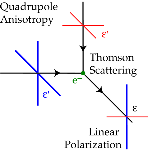
1.3.3 Description of CMB Polarization

Experimentalists seeking CMB polarization are attempting to measure the scalar fields $Q$ and $U$ at every point on the sky. Because $Q$ and $U$ are dependent on the coordinate system chosen, the universally accepted convention is to use the meridian passing through both the celestial pole and the observation point as the defining axis. This meridian represents the N-S direction for the observation point. If the experiment is such that it measures the temperature of the CMB along a given axis, then the linear Stokes parameters in this universal coordinate system are given by [31]

$$Q = T_{NS}\ -\ T_{EW}$$

$$U = T_{NE,SW}\ -\ T_{NW,SE}\ .$$ (1.10)

However, this is still not the most natural way to express CMB polarization; a much better way uses the fact that a polarization field can be decomposed into two components with special symmetry properties, analogous to the fact that a vector field can be decomposed into a curl-free component and a gradient-free component [44, 46]. These components are typically denoted $E$ and $B$, though some authors also use $C$ and $G$. They each are symmetric under rotations, but $E$ is symmetric under parity (reflection) as well, whereas $B$ is anti-symmetric under parity [45].

(a) Pure +E Hot Spot

(b) Pure -E Hot Spot

(c) Pure +B Hot Spot

(d) Pure -B Hot Spot

Figure 1.6: Hot Spots in E and B. Notice that reflections about any axis through the center of the hot spots leave $E$ unchanged, but take $B\rightarrow-B$. All patterns are symmetric under rotation. Courtesy of Ted Bunn [47].

There are standard formulae to construct $E$ and $B$ maps from $Q$ and $U$ maps; for a good description of this process, see [48]. In general the relationship is nonlocal; that is, the values of $E$ and $B$ at a specific point on the sky are functions of $Q$ and $U$ everywhere on the sky, although areas close to the point in question matter more than areas far from the point in question. Figure 1.6 shows typical pure $E$ and $B$ patterns. The E-modes are symmetric under both rotations and reflections about an axis (parity), while the B-modes, possessing a handedness, are symmetric under rotations, but are anti-symmetric under parity.

1.3.4 Polarization Power Spectra

The power spectra for polarization are most naturally expressed in terms of the $E$ and $B$ modes. The mathematics needed to write down these power spectra will be briefly covered in Chapter 9, where we will see that the power spectra are written directly in terms of the Stokes parameters; in the present section we restrict the discussion to a qualitative description of the power spectra.

There are four power spectra used to characterize the CMB radiation field: $C_{\ell}^{TT}$,$C_{\ell}^{EE}$, $C_{\ell}^{BB}$, and $C_{\ell}^{TE}$. Their construction and description is discussed extensively in [46, 49, 50]. $C_{\ell}^{TT}$ is the usual temperature anisotropy power spectrum, formed from the temperature two-point correlation function. $C_{\ell}^{EE}$ is related to the autocorrelation of the $E$-field; because it has the same parity as $C_{\ell}^{TT}$, there is a non-vanishing correlation between temperature anisotropy and $E$-mode polarization, leading to the cross-correlation power spectrum $C_{\ell}^{TE}$. Finally, there is the autocorrelation of the $B$-modes, yielding the $C_{\ell}^{BB}$ spectrum. Because the symmetry under parity is opposite for $B$ as compared to $E$ or $T$, the last two power spectra, $C_{\ell}^{TB}$ and $C_{\ell}^{EB}$ are zero for the CMB. However, these two power spectra may be non-zero in the presence of foregrounds and hence should still be calculated for real data if possible.

1.4 What do we learn from CMB polarization?

This section will attempt to motivate observations of CMB polarization by reviewing what we can learn from it. However, I only scratch the surface of the mass of literature on the subject. For more interested readers, the following reviews are suggested: Kamionkowski and Kosowsky (1999) review how the CMB relates to particle physics, and discuss the clues to understanding inflation left in CMB polarization [51]; Peterson et al. (1999) discuss the CMB in the post-Planck era, and present a very good initial review of CMB polarization [52]; Hu and White (1997) present an excellent primer on the physics of CMB polarization [45].

Figure 1.7: The State of CMB Polarization: approximate experimental limits on the CMB polarization. The unpolarized power spectrum T is shown in black, while the E and cross-polarization TE are shown in red and blue, respectively. The thin red lines (from botton to top) are for reionization models with $\tau$ values of 0, 0.1, 0.2, 0.3 and 0.4. Notice the generation of the “reionization peak” at $\ell=5-10$ in the models with non-zero $\tau$. The fiducial power spectra T, E and TE are computed using the CMBFAST software designed by Zaldarriaga and Seljak [53], employing cosmological parameters from the concordance model of Wang, Tegmark & Zaldarriaga [24]. The historical limits represent decades of work upon which this thesis builds, and are [6, 29, 30, 28, 31, 38, 32, 35, 36, 54, 33, 37, 38, 39, 40]. Reference “K(01)” is this work, originally published in [41]. The compilation of upper limits was kindly provided by Josh Gundersen. Figure provided by Angelica de Oliveira-Costa.

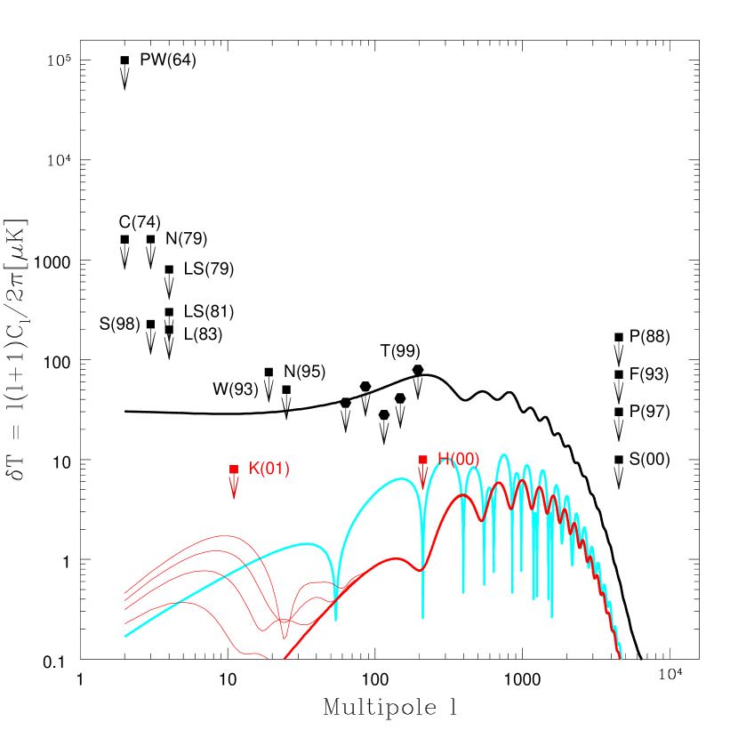
The CMB power spectra depend sensitively on the particular choice of cosmological model and the parameters within it. Figure 1.7 shows sample power spectra calculated for a typical “concordance” model [55], along with the history of polarization upper limits obtained to date. The power spectra were computed with CMBFAST [53]. There are several important pieces of cosmological information that are difficult or impossible to probe with anisotropy alone, but are revealed via polarization studies. We will now discuss a few of the most important of these cosmological questions.

1.4.1 The Effect of Reionization

The universe is currently ionized. By studying the absorption spectra along the line of sight to distant quasars and noticing the lack of HI absorption lines, Gunn and Peterson concluded that the universe is ionized out to a redshift of at least $z\sim 5$ [27]. Very recent results suggest a Lyman-alpha trough in several extremely high redshift systems, implying that the reionization epoch, ended at a redshift of 6–7 [56].

Reionization is a very important process in understanding polarization. After the CMB was released during the era of recombination, it was slightly polarized via Thomson scattering off free electrons at the LSS, as discussed in §1.3.2. However, the free electrons at last scattering are nothing special; any subsequent free electrons encountered by the CMB will additionally polarize the CMB. After recombination, the universe underwent a cosmic “dark age”, in which the CMB propagated freely, but there was no light from stars. A first generation of stars presumably created the radiation that ionized the universe, and led to the Gunn-Peterson observation. We currently believe this happened between a redshift of 6–20.

Reionization has the effect of inducing a “reionization peak” in the E-mode power spectrum [57, 58] at $\ell\lesssim 20$. The true figure of merit is the optical depth to reionization, $\tau$, induced by reionization. The more free electrons between us (as observers) and the LSS, the higher is $\tau$, and hence the more polarized is the CMB. This effect happens primarily at large angular scales, because clumps of free electrons that are closer to us take up a larger angular size on the sky. In models of reionization, it is typically assumed that reionization occurred very quickly, and led to a completely ionized universe; however, it is possible to incorporate a “fraction-polarized” parameter into the models, typically denoted $x$. To convert between the reionization optical depth and the redshift of reionization, $z_{re}$, and $x$ we use [58]

$$\tau\ =\ 0.0015(x)\frac{\Omega_{B}}{0.05}(\Omega_{tot})^{-1/2}\left(\frac{h}{0.65}\right)(1+z_{re})^{3/2}\ ,$$ (1.11)

where $x$ is the fractional ionization ratio, and $\Omega_{B}$, $\Omega_{tot}$ and $h$ have their usual definitions. Recent constraints from anisotropy measurements place $\tau\lesssim 0.20$ [24], although this is a bit deceiving because the effect of reionization is easily mimicked by changing the tensor content of primordial metric perturbations, or the baryonic or cosmological constant contributions to the energy density of the universe. Observations of the $E$-mode CMB polarization can directly constrain the epoch of reionization, because only reionization can generate a low-$\ell$ peak in the $E$-mode polarization power spectrum (see Figure 1.7). Thus, the CMB is a powerful probe of the reionization epoch which ended the cosmic “dark ages”.

1.4.2 A Window on Inflation

The Origin of Structure

The CMB temperature anisotropy is strong evidence for the formation of structure in the universe. We currently believe that large-scale structure arose from tiny density fluctuations in spacetime, that grew via gravitational instability. This growth of structure began perhaps just a little before recombination, in which the universe passed from radiation to matter-dominated; at this time, structures were able to grow. Before that time, structure formation had been inhibited by the photon pressure smoothing out any structures before they could form. As was stated previously, various physical effects, primarily the Sachs-Wolfe effect [15], led to the imprinting of this structure on the CMB during recombination. The level of anisotropy of the CMB today tells us indirectly about the size of density fluctuations at the time of last scattering. However, density fluctuations are just one type of perturbation to the metric of spacetime; along with them, there also could have been gravitational waves. Gravitational waves represent tensor perturbations to the metric. These additional metric fluctuations leave their own imprint on the CMB, but anisotropy measurements alone cannot constrain their relative magnitudes; as we will see, only CMB polarization will help us to determine this information.

Of course, this discussion has only characterized the types of spacetime fluctuations that led to the formation of structure; it begs the question, “Where did the primordial seeds of cosmic structure come from?” Many theories have been proposed, and they all have come from particle physics, such as: primordial adiabatic perturbations due to inflation, topological defects (such as cosmic strings, domain wells, etc), superconducting cosmic strings, axion fluctuations, and many more (see [51] and references therein). These different theories lead to different spectra of metric perturbations, which can be studied through CMB observations. The dominant model is inflation with primordial adiabatic fluctuations. Current observations of the CMB anisotropy, along with observations of large-scale structure via galaxy surveys, have mostly ruled out alternative models to inflation. These models generally require larger temperature anisotropy in the CMB than we see, in order to give rise to the amount of structure observed in the present. Adiabatic fluctuations due to inflation, on the other hand, are quite consistent with the current data.

A full description of inflation is well-beyond the scope of this text; several recent reviews are given in [59, 60, 61]. The basic idea of inflation is that quantum fluctuations grew to cosmological size during a period of exponential expansion very early in the universe (approximately $10^{-38}$ seconds after the Big Bang). Theorists ascribe a field, called the inflaton field, as the cause of inflation. Typically, this field is not in its lowest-energy state at the time of the Big Bang; instead, it “rolls” from this initial state down its potential curve into a lower energy state. This changing of states by the inflaton field releases massive quantities of energy that drives the rapid expansion of the universe.

Figure 1.8: Constraints on the Inflaton Potential from CMB polarization, in the $r$-$n_{s}$ parameter space, where $n_{s}$ is the spectral index for scalar fluctuations, and $r$ is the tensor-to-scalar amplitude ratio, measured at the quadrupole. Simulated $2\sigma$ error ellipses that would be obtained by the Planck Surveyor (without and with polarization), and an experiment with three times the sensitivity of Planck. This assumes an inflationary model with $r=0.01$ and $n_{s}=0.95$ and an optical depth to the surface of last scatter of $\tau=0.05$. Shaded regions indicate the predictions of various inflationary models. Solid horizontal line indicates the regions of this parameter space that would be accessible with a polarization experiment with 30 times the sensitivity of Planck[62]. This figure is illustrative of the gains CMB polarization may provide over the next decade. Courtesy of William Kinney [63].

Constraining the Inflaton Potential

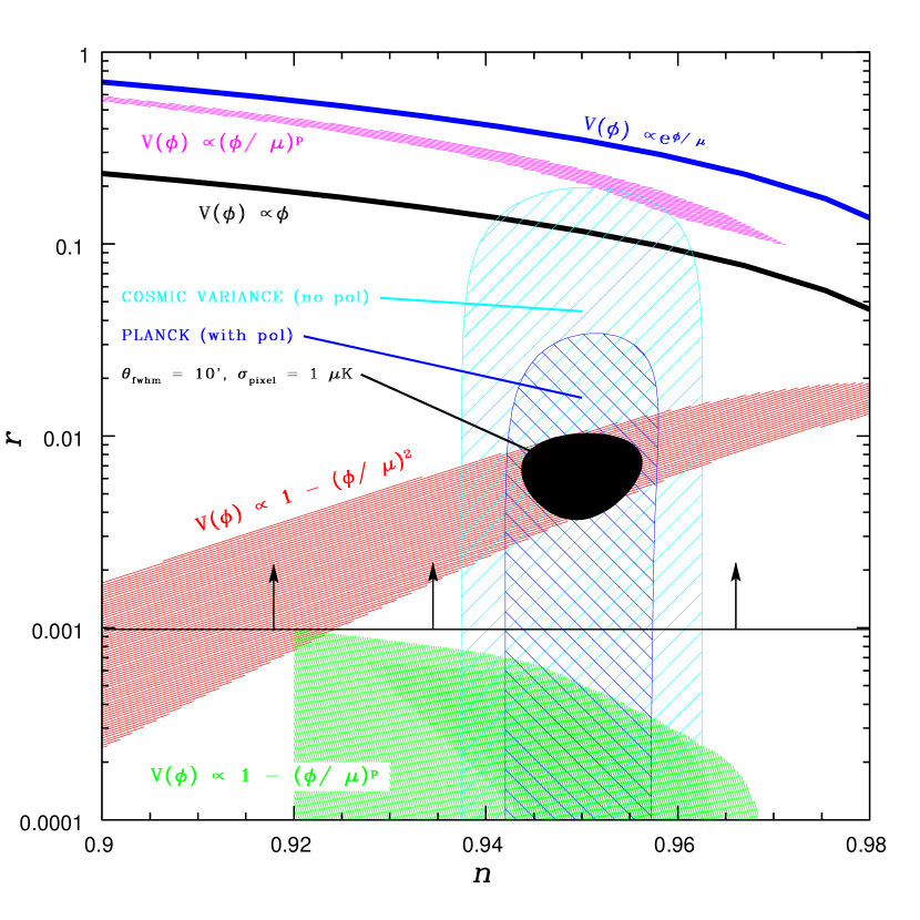
One of the most important aspects of any inflationary theory is the shape of the inflaton potential. This characteristic shape is related to the tensor-to-scalar amplitude ratio, $r$, one of the standard parameters for inflation. Figure 1.8 shows a typical inflation parameter space, $r$ vs. $n_{s}$ (the spectral index of scalar perturbations ). This figure illustrates the utility of polarization measurements; without polarization measurements, inflation can barely be constrained at all, but with polarization, large classes of inflationary models can be excluded. This is because gravitational waves leave a characteristic signature in the CMB polarization. Gravitational waves are tensors and hence have a “handedness” (unlike scalar perturbations), which will lead directly to $B$-mode CMB polarization (recall, $E$-modes have no handedness). In actuality, tensors lead to roughly equal parts $E$ and $B$ modes, but scalar perturbations generate only $E$-modes. Thus, measurement of $B$-modes in the CMB not only is a “smoking gun” discovery of primordial gravitational waves, but also it helps us directly constrain theories of inflation, which set the ratio of tensor-to-scalar metric fluctuations.

The Energy Scale of Inflation

However, we can even go a little further with $B$-modes. It turns out that the energy scale at which inflation occurs imprints itself in the amplitude of $B$-modes; this amplitude is roughly proportional to the square-root of the energy scale of inflation. Most scientists guess that this energy is roughly at the Planck scale, and is due to some Grand-Unified Theory (GUT) phase transition, which sets the energy scale at $\sim$ $10^{19}$ $GeV$. However, some new physics at lower energies could also have led to inflation, making the amplitude of $B$-modes correspondingly lower. Generally, it is believed that a next-generation satellite designed specifically for CMB polarization will be able to see the $B$-modes if inflation occurred at the GUT scale; their absence would indicate new physics at lower energies [51].

Adiabatic vs. Isocurvature Fluctuations

The most common inflationary theory holds that the scalar density perturbations were adiabatic; that is, density perturbations with an equal fraction in number-density for each particle species in the Universe. However, other types of scalar fluctuations are also possible, namely isocurvature perturbations which lead to differences in the number densities of different species in the universe. Isocurvature fluctuations generate a universe where different patches have different ratios of particle densities, which directly leads to pressure differences in the universe, although the universe every maintains a flat geometry (hence the name “isocurvature”). When two initially causally disconnected regions come into contact with each other, their pressure differences will drive the motions of matter, which in turn seeds large-scale structure. This structure will imprint itself on the CMB in the same way that adiabatic density fluctuations will, but in general they lead to slightly different CMB power spectra. Observations of CMB anisotropy have ruled out isocurvature fluctuations as the only source of density fluctuations, but it is still possible that there was a mixture of adiabatic and isocurvature fluctuations.

In general, observations of CMB polarization can help characterize the amount of isocurvature fluctuations, because these fluctuations lead to somewhat different polarization patterns than do adiabatic fluctuations, and these differences are primarily evident at large angular scales [64]. Current parameter constraints from CMB anisotropy assume purely adiabatic density fluctuations; however, it has recently been shown that constraints on cosmological parameters become significantly worsened when a mixture of adiabatic and isocurvature perturbations is allowed [65]. Thus, observations of CMB polarization will constrain the type of initial density fluctuation, and greatly aid in the process of parameter extraction from anisotropy data.

1.5 Summary

In this chapter, we have seen that the CMB polarization potentially provides a wealth of information. In addition to helping further constrain the usual cosmological parameters, CMB polarization can also constrain reionization, thus opening up a window on the cosmic “dark ages”. However, not only does the CMB open up this window, but by viewing gravitational waves via polarization $B$-modes, we potentially have a direct view of events occurring at the beginning of inflation, at $10^{-38}$ seconds after the Big Bang itself! This is because gravitational waves are not affected by ionized matter, and survive the expansion unaffected until they are imprinted upon the CMB. Hence, CMB polarization is truly a new window on the universe.

This work describes a ground-based experiment, polar(Polarization Observations of Large Angular Regions), which searched for CMB polarization during the spring of 2000 from Madison, Wisconsin. The rest of this thesis is organized as follows. In Chapter 2, I describe the problem of galactic foregrounds and their potential impact on CMB polarization experiments. Chapter 3 introduces a new formalism for analyzing microwave polarimeters, and motivates the design of the polar radiometer. In Chapter 4, I present an overview of the instrument. Chapter 5 discusses the calibration of the instrument, while Chapter 6 gives an overview of the year 2000 observations and the climate conditions of the telescope location. Chapter 7 discusses data selection, Chapter 8 presents the mapmaking procedure that was used to construct maps from the data, and finally, Chapter 9 covers the analysis used to set limits on CMB polarization. Finally, let me point the reader’s attention to the polar glossary (Appendix A), which defines several terms used in this work.

Chapter 2 Foreground Radiation

The potential accomplishments of CMB polarization studies must be taken with a grain of salt, however, due to the possible obscuration of CMB polarization by polarized galactic foregrounds. This is especially likely at larger angular scales where the CMB signal is expected to be very small, and several foregrounds are expected to have a falling power angular spectrum (thus being worse at larger angular scales).

While there are many dark sections in the sky where CMB anisotropy dominates galactic emission at the relevant microwave frequencies, it is simply not known the extent to which polarized foregrounds will pose a problem to CMB polarization searches. To truly characterize foregrounds for polarization, we must understand them in terms of their $E$ and $B$ mode contributions, their behavior in $\ell$-space, and their intensity and polarization dependence on frequency. The primary foregrounds to be concerned with at microwave frequencies are dust emission, bremsstrahlung, and synchrotron radiation.

There is also the question of possible polarized emission by the Earth’s atmosphere. As shown in Chapter 6, there are strong features in the atmosphere that lead to significant emission at microwave frequencies. A polarization fraction of even one part in one million would lead to an emission of 20 $\mu K$ which would entirely swamp the tiny cosmological signal from the CMB. As far as is known, the mechanism producing the highest polarization level from the Earth’s atmosphere is the Zeeman splitting of oxygen lines by the Earth’s $\sim$ 0.5 Gauss magnetic field, but Keating (2000) shows that this leads to less than $10^{-8}$ fractional polarization. There is also the possibility of Faraday rotation of the plane of CMB (or foreground) polarization due to the magnetic field of the Earth, but this can be shown to be less than 0.01^∘ at frequencies above 25 GHz [58], where most CMB observations occur. Thus, although the atmosphere adds noise to our experiment, we can neglect the concerns of polarized emission and Faraday rotation by the atmosphere.

Figure 2.1: Estimated Spectra of Polarized Microwave Foregrounds. The synchrotron spectrum is normalized to the rms brightness temperature of synchrotron at 19 GHz (de Oliveira-Costa et al., 1998) and assumes 30% polarization. The bremsstrahlung spectrum is normalized to 30 $\mu K$ at 10 GHz (Davies and Wilkinson, 1999) and assumes a 10% polarization. The spinning dust spectrum proposed by Draine and Lazarian (1998) is shifted by 2/3 to lower frequencies as prescribed by (de Oliveira-Costa, 1999) and assumes 3% polarization. The thermal dust spectrum assumes 5% polarization (Prunet and Lazarian, 1999), a dust temperature of 18 K, an emissivity index of 1.8 (Kogut et al., 1996) and uses 3 $\mu K$/MJy/sr to scale typical degree scale rms values (of 0.5 MJy/sr) at 100 microns to 90 GHz. The CMB E-polarization spectrum is assumed to be $10^{-6}$ of the CMB brightness spectrum and the CMB B-polarization is assumed to be 0.1 of the E-polarization spectrum. Three frequency bands ($K_{a}$, W and D) are shown above the spectra.

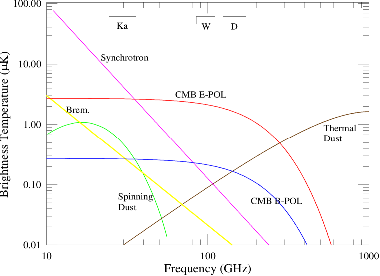
Figure 2.1 is a good introduction to polarized microwave foregrounds. It shows that polarized synchrotron and dust are the most troublesome foregrounds. Dust exhibits three possible sources of polarized emission, thermal emission due to the vibration modes in the dust, non-thermal electric dipole emission due to rotating dust grains, and magnetic dipole-emission due to magnetic grains. At 30 GHz, the dominant foreground is expected to be synchrotron, although in certain areas spinning dust grains could also pose a threat. Bremsstrahlung (free-free) radiation is not expected to be polarized at any significant level [58], and studies show that in most areas, its intensity is completely dominated by that of synchrotron (e.g. , de Oliveira-Costa (2001) [66]). We will now discuss each of these foregrounds, as they relate to polar, in more detail.

2.1 Galactic Synchrotron

As is shown in Figure 2.1, synchrotron will likely be the dominant polarized foreground at 30 GHz. For a fairly comprehensive review to the issue of synchrotron as a foreground, the reader is referred to Cortiglioni and Spoelstra (1995) [67]. Synchrotron emission occurs when a charged, relativistic particle is travelling through a local magnetic field . The charged particle will not have its energy changed by interaction with the field (magnetic fields do no work!), but it will be caused to spiral about the magnetic field lines. This radial acceleration causes the charged particle to radiate, and the resulting radiation is in general polarized, and has a frequency distribution that depends on both the charge and speed of the particle, as well as the magnetic field strength. A collection of particles moving at different speeds will give rise to a broad spectrum of radiation.

Thus, synchrotron is highest in areas of high magnetic field, as well as high concentrations of charged particles along the line-of-sight. It is strongest in the galactic plane, but is present even at high galactic latitudes [68]. Synchrotron radiation at high galactic latitudes follows a rough power-law form:

$$T_{ant}\propto\nu^{\alpha}\ ,$$ (2.1)

where $\alpha$ is called the spectral index of synchrotron. The primary species dominating synchrotron radiation at higher frequencies (i.e. greater than 1 GHz) is cosmic-ray electrons. The energy distribution of these electrons largely determines the spectral index [69]. At lower frequencies, the spectral index of synchrotron is roughly $-2.8\pm 0.1$ [70]. Above 10 GHz there is strong evidence for a steepening spectral index, to as high as -3.5 or so [70, 66]; this is due to the rapid drop-off in relativistic electrons above about 15 GeV [71, 72, 73]. It should also be noted that many surveys indicate a significant variation (up to 0.3) of the value of the synchrotron spectral index [73, 68].

Synchrotron is elliptically polarized by its very nature. This polarization has a maximum of about 75%, and this maximum polarization fraction is related to the spectral index via $\Pi=\frac{3\alpha+3}{3\alpha+1}$ [67]. Brouw and Spoelstra (1976) attempted to map polarized synchrotron emission at 1411 MHz [74]. The resulting maps are very under-sampled and are subject to non-negligible Faraday depolarization (which goes as $\nu^{-2}$), but still indicate 20-30% polarization at high galactic latitudes, $|b|>30^{\circ}$ [74]. Some studies have found regions with up to 72% polarization; 30-50% is a common maximum polarization in various high-latitude features [75].

In terms of power spectra, the spatial variation of galactic synchrotron is also modelled as a power law, with $C_{\ell}\propto\ell^{-\beta}$. Data sets such as the Haslam 408 MHz survey and the Parkes southern hemisphere survey indicate $2.4<\beta<3.0$ ([76] and references therein). For polarized synchrotron, much less is known. Polarization maps at 2.4 GHz by the Parkes survey [77] indicate $\beta\sim 1.0$, a much less steep index that would imply polarized synchrotron is not as bad at large angular scales as small [76]. Recent work by Baccigalupi et al. (2001) analyzing polarization surveys indicates a steeper index, $\beta=1.8\pm 0.3$ for $\ell>100$, and steepening at lower $\ell$-values, towards a $\beta$ of $\sim$ 3 [78].

Clearly, much work remains to be done in this area, but surely synchrotron could be a big problem for polar. In order to further understand the potential effects of synchrotron on our experiment, we extrapolated the Haslam data to higher frequencies using the knowledge available of the spectral index, and assumed a fairly high polarization of 50%; the results are shown in Figure 2.2. The map has been smoothed with our 7^∘ beam. The bright source at RA 20h is Cygnus A, the second brightest radio source in the sky. There is obviously a large chance we should see synchrotron. In order to limit our sensitivity to synchrotron, we restricted our CMB analysis to right ascensions in the range $7.5h<RA<18h$, where polarized synchrotron should be 20-40 $\mu K$ or less in our beam. The reader should note that this is much larger than the $\sim$ 0.1-2 $\mu K$ signal we are attempting to see!

Figure 2.2: The Haslam 408 MHz data [79], convolved with a 7^∘ beam, between declinations 30^∘ and 55^∘. The strip covered by polar’s FWHM is shown between the dashed lines. The map was obtained by extrapolating to 31 GHz with a spectral index of -2.8 up to 7.5 GHz, and -3.0 at higher frequencies, based on [70]. 50% polarization has been assumed. Intensity scaling is logarithmic. The bright feature at $\sim$ 20h is Cygnus A. Data from http://skyview.gsfc.nasa.gov.

The usual technique to subtract foregrounds is to understand their spectral behavior, and make multifrequency measurements of the same area of the sky. This will be difficult with the polar data, but not impossible as we do make measurements at three different (albeit closely spaced) frequencies. Preliminary work on this front was done by Keating et al. (1998) based on the work of Dodelson (1997) [58, 80]. More advanced subtraction techniques that take into account the spatial structure of foregrounds were developed by Tegmark and others [81, 82, 83, 76]. Further discussion of this topic as it relates to polar will await inspection of our data (for the reader that cannot wait, skip to Chapter 9).

2.2 Free-free Emission

Bremsstrahlung (free-free) emission is an important process at radio frequencies, though it is often dominated by synchrotron radiation. It is the well-understood process of an electron passing close to a proton in an ionized medium; the particles are accelerated as they pass near each other, and hence radiate. Bremsstrahlung radiation is well-described as a power law, with the intensity of radiation proportional to $\nu^{-\alpha}$, with $\alpha=2.15\pm 0.02$ in most regions of the sky [76]. Free-free emission is intrinsically unpolarized [69], but can become polarized by its parent HII region (where it is produced) via Thomson scattering off the electrons in the cloud; recall that this is the same process by which the CMB is polarized at last scattering. It is expected that in the most extreme circumstances, this would lead to a 10% polarization fraction [58, 84]. Because synchrotron emission dominates bremsstrahlung at almost all frequencies and locations on the sky, and because it exhibits much greater polarization, we will not consider free-free emission further.

2.3 Dust Emission

2.3.1 Anomalous Emission at Low Frequencies

Dust emission is complicated. Until recently, the emission of dust was assumed to be exclusively thermal (vibrational). Cross-correlations of the COBE DIRBE data with IRAS support a dust emission model where most dust is at a stable temperature of approximately 20 K [85]; in the Rayleigh-Jeans portion of its spectrum, this corresponds to a rapidly falling spectrum, such that below 90 GHz dust emission was historically considered unimportant as compared to synchrotron (see Figure 2.1).

However, multiple experiments at frequencies between 10 and 36 GHz now support an additional mechanism of dust emission that is less well understood. In 1995, Leitch et al. reported an excess emission (inconsistent with synchrotron) at 14.5 and 32 GHz, and a large correlation with IRAS far-infrared data at 14.5 GHz [86]. The excess emission was initially attributed to free-free emission, but that hypothesis was later ruled out on energetic grounds [87]. The large correlation with IRAS (which is completely dominated by dust emission) suggests a common emission source.

More recently, a strong correlation with IRAS data for both Tenerife data at 10 and 15 GHz [88], as well the 19 GHz maps of Cottingham [89] has been noted. In the former case, it was compared to maps of $H\alpha$ (a good tracer of free-free) to test the free-free hypothesis, and it was found that free-free emission is a factor of ten too small to explain the emission [90]. The conclusion drawn is that the correlation with IRAS data (dominated by dust emission) is due to some previously unknown dust emission mechanism [66].

Recently, new data by Finkbeiner et al. show a direct detection of excess emission at low frequencies in two point sources [91]. This is in contrast to all previous sources of evidence, which were statistical in nature. The Finkbeiner team surveyed ten fields at 5, 8, and 10 GHz with the 140-foot Greenbank telescope. In most cases the observed emission was consistent with free-free or bremsstrahlung, and had a falling spectrum with frequency. However, two fields show a rising spectrum with frequency (consistent with the dust emission mechanisms described below), and one of these two fields is inconsistent with free-free or synchrotron at the $\sim$ $10\sigma$ level. What could this new emission mechanism be?

2.3.2 Dust Emission Mechanisms at Low Frequencies

Electric Dipole Emission from Spinning Grains

To explain the anomalous dust emission at low frequencies, Draine and Lazarian have proposed two new emission mechanisms for dust: electric dipole emission from small, spinning grains [87] (hereafter DL98), and magnetic dipole emission by magnetic grains [92]. In the former hypothesis, ultra-small grains emit via electric dipole radiation because they are spinning rapidly (at frequencies of 10–30 GHz!). A dust particle with electric dipole moment $\mu$ and angular rotational frequency $\omega$ will exhibit emission proportional to $\mu^{2}\omega^{4}/c^{3}$; the total emission is this factor times the number of emitting grains $n_{g}$ along the line of sight.

There are many mechanisms that contribute to the rotational velocity of dust grains, but in general small ($N<150$ atoms) dust grains can be spinning rapidly due to collisions with fast-moving neutrals and ions in the ISM. Grains can acquire a net dipole moment through two means. First, grains are expected to have an inherent dipole moment due to the dipole moments of their chemical bonds, if they are not completely symmetric molecules. Secondly, if the grain is charged and the center-of-charge does not coincide with the center-of-mass, this will induce a dipole moment. DL98 estimated the parameters $\omega$, $\mu$ and $n_{g}$ for the dust particles that would dominate the overall emission. The resulting spectrum is a blackbody-like curve that peaks somewhere from $15-25$ GHz; a typical spectrum is shown in Figure 2.1 as the “spinning dust” model.

In terms of polarization, microwave emission from the spinning grains is expected if the grains are aligned. Lazarian and Prunet reviewed this process recently in [93]. Grains in the galactic magnetic field will experience a torque that tends to align their angular momenta with the magnetic field via the paramagnetic dissipation mechanism of Davis-Greenstein [94]. It turns out this leads to essentially no polarization at frequencies of 10 GHz, as shown in Figure 2.3.

Figure 2.3: Polarization for both the resonance relaxation theory of Draine and Lazarian and Davis-Greenstein relaxation for dust grains as a function of frequency (from [95]). For resonance relaxation, saturation effects are neglected, which means that the upper curves correspond to the maximal values allowed by the paramagnetic mechanism. Even in the worst case, polarization from spinning dust grain emission is expected to be very small.

However, Lazarian and Draine (2000) point out that this picture is incomplete, and propose a modification to the theory to account for an extra alignment mechanism, called “Barnett Magnification” [95]. This effect involves spontaneous magnification of the rotating grain in a local magnetic field, and leads to paramagnetic relaxation, which the authors called “resonance relaxation”. However, this mechanism only marginally increases the polarization of spinning grains. As shown in Figure 2.3, in the polar frequency range of 26–36 GHz, the polarization fraction is less than 1% for resonance relaxation, and is almost exactly zero for the Davis-Greenstein theory. Thus, electric dipole emission from spinning dust grains is not likely to be a problem for polarization measurements, although until accurate measurements of polarization are made at the frequency where this emission peaks ($\sim$ 15 GHz), the picture will not be complete.

2.3.3 Magnetic Dipole Emission from Dust

Lazarian and Prunet (2001) point out that there is another, often-overlooked dust emission mechanism also relevant at low frequencies: thermal fluctuations of magnetization in individual dust grains. This leads to magnetic dipole emission. Often the magnetic characteristics of dust are neglected at higher frequencies when calculating their emission properties; typically electric dipole emission leads to the usual “thermal” (vibrational) emission of dust that is so strong at higher frequencies.

Draine and Lazarian (1999) calculated the expected emission from magnetic grains as a function of frequency; the emission is strongly dependent on what magnetic species make up the grains [92]. The materials they considered were metallic iron and nickel, and various iron-containing compounds. The main result was that this emission could be important for frequencies between 10 and 100 GHz, although there is strong variability in the emission curves depending on what types and amounts of magnetic materials are included in the grains. They note, however, that the anomalous emission reported by Kogut et al. (1996) [85] at 90 GHz reported by the DMR can be explained by magnetic emission if 5% of interstellar iron is locked up in dust.

These arguments then point to a potentially complicated picture of dust, where at some frequencies, three different emission mechanisms could be important. Regarding polarization, it is possible that the magnetic mechanism can lead to emission that is up to 30–40% polarized, depending again on the magnetic species dominating dust grains. This polarization results from alignment with the local magnetic field, and due to their magnetization it is possible that a large fraction of grains are aligned. Thus, it is conceivable that at frequencies around 30 GHz, dust emission could be dominated by rotational emission in intensity, but by magneto-dipole emission in polarization [93].

2.3.4 Dust Templates and Conclusions

It is interesting to look at a template of dust emission in our observation region; this is shown in Figure 2.4 for the DIRBE 100 $\mu$m data [96]. We can see the same strong emission features due to the galaxy as in the synchrotron map (Figure 2.2), and in between the galactic features there is much less emission.

Figure 2.4: DIRBE 100 $\mu m$ emission map, convolved with a 7 ^∘ beam, between declinations 30^∘ and 55^∘. The strip covered by polar’s FWHM is shown between the dashed lines. Intensity scaling is logarithmic. Data from http://skyview.gsfc.nasa.gov.

We can conclude from this map that the only form of dust emission capable of affecting polar is magneto-dipole emission, unless the theories regarding polarized spinning grain emission are inaccurate or incomplete. This is because the DIRBE 100 $\mu m$ data show a level of 3-5 MJy/sr in our beam path at high galactic latitudes ($|b|>25^{\circ}$). This corresponds to roughly 10-20 $\mu K$ of emission at 100 $\mu m$. Using the Rayleigh-Jeans law, this thermal emission can be extrapolated to $\lambda=1\ cm$, giving roughly 0.1–0.2 $\mu K$ of thermal emission. A typical spinning dust scenario implies as much as 50 times more emission at 30 GHz from spinning dust as from thermal emission in certain regions of the sky [90]. This implies perhaps 5–10 $\mu K$ of emission from rapidly rotating dust grains in intensity. Assuming a fairly worst-case scenario of 1% polarization, this leads to around 0.1 $\mu K$ polarized emission. Compare this to the results of Figure 2.2, which shows typical intensities in the same region of the sky of 20–50 $\mu K$, and could be as much as 75% polarized! Even if the excess emission reported in [90] is purely magneto-dipole, this is expected to be at most 20–40% polarized (and is probably much less). This would put polarized dust emission at a level on par with weakly (10%) polarized synchrotron with a steep spectral index.

Thus for most scenarios, we expect the dominant foreground for polar to be synchrotron. This is not necessarily bad, because it is still interesting to map out any polarized galactic emission at our relatively under-studied frequency. In addition to any CMB knowledge we reap, it will still be useful to the community to have an enhanced understanding of polarized emission from these various galactic foregrounds.

Chapter 3 Polarimeter Analysis Formalism

3.1 Description of the Formalism

There are many possible radiometric schemes to measure microwave polarization. In order to achieve the low noise levels necessary to see CMB polarization, however, the system must not only be extremely sensitive, but also extremely stable. It should be insensitive to gain drifts in the front-end amplifiers and have 1/f noise that is as low as possible.

A radiometer can in principle be designed to measure all four Stokes parameters. For CMB polarization, it is typically desirable to be sensitive to both Stokes Q and U simultaneously; as discussed in Chapter 2, the CMB is expected to exhibit only linear polarization (although this certainly isn’t a strong argument against measuring V). Thus, the polarimeter must be designed with the issue in mind of which Stokes parameters are to be measured. In this chapter, I describe a useful formalism for analyzing the output of polarimeters in terms of the Stokes parameters. The formalism is based upon the Jones’ matrix formalism of polarization, but is a little bit different as we shall see.

3.1.1 Description of Polarized Radiation

The general situation for a microwave polarimeter is that electromagnetic radiation is incident upon a feedhorn antenna. This radiation can be described by its electric field; for a single frequency of this radiation, as in Chapter 1, the electric field can be written as

$$\vec{E} =E_{x}\hat{x}+E_{y}\hat{y} \ ,\ \text{with}$$ (3.1)

$$E_{x} =E_{x_{0}}e^{i(kz-\omega t+\phi_{x})}$$

$$E_{y} =E_{y_{0}}e^{i(kz-\omega t+\phi_{y})} \ .$$

It is implicit that one takes the real part of $\vec{E}$ to obtain the physical field. We can equally well describe this radiation as a complex, 2-element Jones’ vector, or a real, 4-element Stokes vector [97, 98]:

$$|E\rangle\;=\;e^{i(kz-\omega t)}\begin{bmatrix}E_{x_{0}}e^{i\phi_{x}}\\ E_{y_{0}}e^{i\phi_{y}}\end{bmatrix}\qquad\qquad\text{or}\qquad\qquad|E\rangle\;=\;\begin{bmatrix}I\\ Q\\ U\\ V\end{bmatrix}$$ (3.2)

where the Stokes parameters for monochromatic radiation are defined in the usual way [42] as

$$I =\langle E_{x_{0}}^{2}+E_{y_{0}}^{2}\rangle$$ (3.3a)

$$Q =\langle E_{x_{0}}^{2}-E_{y_{0}}^{2}\rangle$$ (3.3b)

$$U =2\langle E_{x_{0}}E_{y_{0}}\cos(\phi_{x}-\phi_{y})\rangle$$ (3.3c)

$$V =2\langle E_{x_{0}}E_{y_{0}}\sin(\phi_{x}-\phi_{y})\rangle\ ,$$ (3.3d)

where $\langle...\rangle$ denotes a time average. For quasimonochromatic light, each component of Equation (3.3) is understood to be averaged over the entire frequency band. However, in this formalism we need only consider one frequency at a time; the final results can then be averaged over frequency space.

3.1.2 The Stokes Operators

It is useful to notice that we can think of the Jones’ vector of a field as a state and describe each Stokes parameter as an $2\times 2$ matrix operator. To evaluate the Stokes parameter of a state $|E\rangle$, we simply follow the procedure from quantum mechanics: $\langle\bf{O}\rangle=\langle E|\bf{O}|E\rangle$, where $\bf{O}$ is the operator in question, and $\langle E|$ is the hermitian conjugate of $|E\rangle$. The correct matrix operators for the Stokes parameters are given by

$${\bf I}\;=\left[\begin{array}[]{cc}1&0\\ 0&1\end{array}\right] {\bf Q}\ =\left[\begin{array}[]{cc}1&0\\ 0&-1\end{array}\right]$$ (3.8)

$${\bf U}\;=\left[\begin{array}[]{cc}0&1\\ 1&0\end{array}\right] {\bf V}\ =\left[\begin{array}[]{cc}0&-i\\ i&0\end{array}\right]\;\;\text{.}$$ (3.13)

The astute reader will notice that these are none other than the Pauli spin matrices, and hence have the following useful properties:

$${\bf I}\;\;\text{is the identity}$$ (3.14a)

$${\bf Q}^{2}\;=\;{\bf U}^{2}\;=\;{\bf V}^{2}\;=\;{\bf I}$$ (3.14b)

$${\bf Q}{\bf U}\;=\;-{\bf U}{\bf Q}\;=\;i{\bf V}$$ (3.14c)

$${\bf U}{\bf V}\;=\;-{\bf V}{\bf U}\;=\;i{\bf Q}$$

$${\bf V}{\bf Q}\;=\;-{\bf Q}{\bf V}\;=\;i{\bf U}$$

Let us verify Equation (3.8) for U as an example.

$$\langle{\bf U}\rangle =\langle E|{\bf U}|E\rangle$$

$$=[E_{x}^{*}\text{,}E_{y}^{*}]\ \left[\begin{array}[]{cc}0&1\\ 1&0\end{array}\right]\ \begin{bmatrix}E_{x}\\ E_{y}\end{bmatrix}$$

$$=E_{x}^{*}E_{y}+E_{y}*E_{x}=2\ \text{\bf{Re}}(E_{x}^{*}E_{y})$$

$$=2\ \text{\bf{Re}}(E_{x_{0}}E_{y_{0}}e^{i(\phi_{y}-\phi_{x})})=2E_{x_{0}}E_{y_{0}}\cos(\phi_{y}-\phi_{x})$$

$$=U\;\checkmark$$

as promised. The other Stokes parameter operators likewise yield the desired results from Equation (3.3).

It is worthwhile to evaluate the Stokes parameters in a rotated reference frame. This is a straightforward calculation, but when done in the usual notation of Equation (3.1), the mathematics is cumbersome. The Jones-matrix formalism makes it particularly simple. Let us work out the rotation of Q to demonstrate this. If the rotation matrix corresponding to a rotation by the angle $\phi$ is given by

$$\mathbf{R}(\phi)=\left[\begin{array}[]{cc}\cos{\phi}&\sin{\phi}\\ -\sin{\phi}&\cos{\phi}\end{array}\right]\text{,}$$ (3.15)

then the operator ${\bf Q}^{\prime}$ as seen in the rotated frame is given by ${\bf Q}^{\prime}=\mathbf{R}^{\dagger}(\phi){\bf Q}\mathbf{R}(\phi)$. Thus,

$${\bf Q}^{\prime} =\left[\begin{array}[]{cc}\cos{\phi}&-\sin{\phi}\\ \sin{\phi}&\cos{\phi}\end{array}\right]\left[\begin{array}[]{cc}1&0\\ 0&-1\end{array}\right]\left[\begin{array}[]{cc}\cos{\phi}&\sin{\phi}\\ -\sin{\phi}&\cos{\phi}\end{array}\right]$$

$$=\left[\begin{array}[]{cc}\cos{\phi}&-\sin{\phi}\\ \sin{\phi}&\cos{\phi}\end{array}\right]\left[\begin{array}[]{cc}\cos{\phi}&\sin{\phi}\\ \sin{\phi}&-\cos{\phi}\end{array}\right]$$

$$=\left[\begin{array}[]{cc}\cos^{2}{\phi}-\sin^{2}{\phi}&2\sin{\phi}\cos{\phi}\\ 2\sin{\phi}\cos{\phi}&\sin^{2}{\phi}-\cos^{2}{\phi}\end{array}\right]$$

$$=\left[\begin{array}[]{cc}\cos{2\phi}&\sin{2\phi}\\ \sin{2\phi}&-\cos{2\phi}\end{array}\right]$$

$$=\cos{2\phi}\left[\begin{array}[]{cc}1&0\\ 0&-1\end{array}\right]+\sin{2\phi}\left[\begin{array}[]{cc}0&1\\ 1&0\end{array}\right]$$

$$={\bf Q}\cos{2\phi}+{\bf U}\sin{2\phi}\;\;\text{.}$$

Working these rotations out for each of the Stokes parameters, one obtains the usual result that

$${\bf I}^{\prime} ={\bf I}$$ (3.16a)

$${\bf Q}^{\prime} ={\bf Q}\cos{2\phi}+{\bf U}\sin{2\phi}$$ (3.16b)

$${\bf U}^{\prime} =-{\bf Q}\sin{2\phi}+{\bf U}\cos{2\phi}$$ (3.16c)

$${\bf V}^{\prime} ={\bf V}\;\text{.}$$ (3.16d)

3.1.3 Radiometric Operators

Thus far we have described generic electric fields as Jones vectors, and Stokes parameters as operators that can tell us what each Stokes parameter for a given state is. Next reconsider the initial electric field state entering a polarimeter. After passing through the feedhorn antenna, an orthomode transducer (OMT) separates the two polarizations and sends them down different rectangular waveguides, which we refer to as arms of the polarimeter (see Figure 3.1). However, we can still consider these two polarizations together as part of the same state, described by the same Jones vector as before OMT traversal.

The next piece of the formalism, then, is to construct operators ($2\times 2$ matrices) representing the action of various radiometric components (such as amplifiers, magic tees, phase shifters, etc.) on the initial state. Each successive component will then act on the incoming state, and produce a new output. We can describe the action of each component as a matrix scrambling together these two fields, and creating two outputs every time. We can then describe the entire polarimeter as a single $2\times 2$ matrix, itself a sum of the four Stokes parameters (in operator form). It is these Stokes parameters that the polarimeter will be capable of detecting.

Component	Schematic/Symbol	Operator
Name		Equivalent
Orthomode Transducer		$\left[\begin{array}[]{cc}{1}&{0}\\ {0}&{1}\end{array}\right]$
Septum Polarizer (Circular Hybrid Polarizer)		$\frac{1}{\sqrt{2}}$$\left[\begin{array}[]{cc}{1}&{i}\\ {i}&{1}\end{array}\right]$
Amplifiers		$\left[\begin{array}[]{cc}{G_{1}}&{0}\\ {0}&{G_{2}}\end{array}\right]$
Phase Shifters		$\left[\begin{array}[]{cc}{e^{i\phi_{1}}}&{0}\\ {0}&{e^{i\phi_{2}}}\end{array}\right]$
Magic Tee (180∘ Hybrid)		$\frac{1}{\sqrt{2}}$$\left[\begin{array}[]{cc}{1}&{1}\\ {1}&{-1}\end{array}\right]$
Short-Slot Hybrid Coupler (90∘ Hybrid)		$\frac{1}{\sqrt{2}}$$\left[\begin{array}[]{cc}{1}&{i}\\ {i}&{1}\end{array}\right]$
Quarter-Wave Plate at Angle $\theta$	N/A	$\frac{1}{\sqrt{2}}\left[\begin{array}[]{cc}-\cos{2\theta-i}&\sin{2\theta}\\ \sin{2\theta}&\cos{2\theta}-i\end{array}\right]$
Detection Devices
Diode		$\left[\begin{array}[]{cc}{1}&{0}\\ {0}&{0}\end{array}\right]$ or $\left[\begin{array}[]{cc}{0}&{0}\\ {0}&{1}\end{array}\right]$
Multiplier		$\left[\begin{array}[]{cc}{0}&{1}\\ {1}&{0}\end{array}\right]$  = U

Table 3.1: Schematics and matrix operators for selected radiometer components.

Table 3.1 shows various radiometric components, their electrical representation, and their corresponding operator matrix. From the table we see that the basic operators take in each of the two arms of the radiometer, and produce some linear combination of those fields in each output arm: $|E_{out}\rangle={\bf M}|E_{in}\rangle$, where ${\bf M}$ is the matrix operator for that component. “Detector Devices” work the same but have only one (scalar) output, so their formalism is $\texttt{{v}}=\langle E_{in}|{\bf D}|E_{in}\rangle$, where $\mathbf{D}$ is the matrix operator for that detector, and v represents the scalar output from the detector. Hence, the formalism can output what one actually measures, i.e. a voltage. The entire procedure can be described as follows:

1. OMT creates the state $|E_{0}\rangle$

2. Radiometric elements act to produce the final state before detection,
   $|E_{f}\rangle=\ldots\mathbf{M_{3}M_{2}M_{1}}|E_{0}\rangle\;\equiv\;{\bf P}|E_{0}\rangle$

3. Detector D produces a scalar output v $\propto\langle E_{f}|{\bf D}|E_{f}\rangle$ = $\langle E_{0}|{\bf P}^{\dagger}{\bf D}{\bf P}|E_{0}\rangle$ =
   $\langle E_{0}|\mathbf{M_{1}}^{\dagger}\mathbf{M_{2}}^{\dagger}\mathbf{M_{3}}^{\dagger}\ldots{\bf D}\ldots\mathbf{M_{3}}\mathbf{M_{2}}\mathbf{M_{1}}|E_{0}\rangle$

4. The full gambit of matrix operations for a given polarimeter can be written as a linear combination of Stokes parameters, ${\bf P}^{\dagger}{\bf D}{\bf P}=c_{I}{\bf I}+c_{Q}{\bf Q}+c_{U}{\bf U}+c_{V}{\bf V}$.

5. The $c_{i}$ coefficients then describe the polarimeter’s sensitivity to each of the Stokes parameters.

3.1.4 Comments on the Operators

There are several other things to note from Table 3.1. First, phase shifts common to both polarimeter arms are not shown, as they are immaterial; only phase differences between the two arms matter. Second, devices that neither amplify nor attenuate have unitary matrices, representing the conservation of power. Diagonal matrices do not mix the signals from the two arms; this occurs when the signal arms do not cross (such is in amplifier chains in the front-end).

It is interesting to see how some of these components behave. A septum polarizer is mathematically equivalent to a 90^∘ hybrid junction; the septum polarizer acts on a combined wave in square waveguide, while the 90^∘ hybrid acts on the already-split polarizations, but the outputs are identical. Thus, we conclude a septum polarizer is the same as an OMT followed by a 90^∘ hybrid.

Another comment is on the quarter-wave plate; when mounted with its axis at 45^∘ or 135^∘ to the OMT, its effect is equivalent to that of a 90^∘ hybrid. When mounted at 0^∘ or 180^∘  though, its effect is to add a 90^∘ relative phase shift between the two polarimeter arms (which can be useful in certain situations).

3.1.5 Phase Chopping

Many coherent radiometers employ some type of chopping scheme within the radiometer to reduce offsets. This is often accomplished by electronically chopping a phase shifter in one or both arms of the signal chain; examples of radiometers that employ this technique are MAP and PIQUE, as well as polar [99, 40]. Electronically switching phase shifters are now available in waveguide at frequencies up to 100 GHz [100]. Typically the relative phase difference between two arms is chopped between 0^∘ and 180^∘.

3.2 A Correlation Polarimeter

Figure 3.1: Sample polarimeter configurations. (a) depicts the basic correlation polarimeter, which is sensitive only to U; (b) shows a correlation polarimeter that simultaneously detects both Q and U. The Septum Polarizer is equivalent to a quarter-wave plate mounted at 45^∘ followed by an OMT, or an OMT followed by a 90^∘ hybrid tee; (c) is a basic pseudo-correlation polarimeter, which also is only sensitive to U. In all cases we assume phase-sensitive detection with a phase chop of $\phi_{2}-\phi_{1}=0,180^{\circ}$, which drastically reduces 1/f noise introduced by the front-end amplifiers.

3.2.1 Description

Let us now apply this formalism to several different polarimeter configurations, to see which Stokes parameters these configurations actually detect. Our first example is the basic correlation polarimeter, as shown in Figure 3.1(a). Radiation enters an axially symmetric feed, and passes through an OMT. The OMT sends the x-component of the input field down one arm, and the y-component down the other. Each signal is then amplified and then phase-shifted, although as usual only the relative phase shift between the two arms is important; in this idealized approach, we ignore the differential phase shifts associated with different frequencies across the band. Finally, the two signals are multiplied with some type of correlating element.

3.2.2 Analysis

Let us now analyze the behavior of this radiometer. In our formalism, the OMT does nothing to the Jones vector $|E_{in}\rangle$. The action of the amplifiers and phase shifters produces a state $|E_{f}\rangle$ entering the correlator given by

$$|E_{f}\rangle\; =\;\mathbf{\Phi}\;\mathbf{G}\;|E_{in}\rangle$$

$$=\;\left[\begin{array}[]{cc}1&0\\ 0&e^{i\Delta\phi}\end{array}\right]\left[\begin{array}[]{cc}G_{1}&0\\ 0&G_{2}\end{array}\right]|E_{in}\rangle$$ (3.21)

$$=\;\left[\begin{array}[]{cc}G_{1}&0\\ 0&G_{2}e^{i\Delta\phi}\end{array}\right]|E_{in}\rangle$$ (3.24)

$$\equiv\;{\bf P}\;|E_{in}\rangle\;\;\text{.}$$ (3.25)

where P simply encodes the action of all the components of the radiometer preceding detection. Now this state enters the correlator to produce a voltage v. Referring back to Table 3.1, we see that a correlator has the action of the U operator, so:

v $$\propto\langle E_{f}|\;{\bf U}\;|E_{f}\rangle=\langle E_{in}|\;{\bf P}^{\dagger}{\bf U}{\bf P}\;|E_{in}\rangle$$

$$=\langle E_{in}|\left[\begin{array}[]{cc}G_{1}&0\\ 0&G_{2}e^{-i\Delta\phi}\end{array}\right]\left[\begin{array}[]{cc}0&1\\ 1&0\end{array}\right]\left[\begin{array}[]{cc}G_{1}&0\\ 0&G_{2}e^{i\Delta\phi}\end{array}\right]|E_{in}\rangle$$ (3.32)

$$=\langle E_{in}|\left[\begin{array}[]{cc}0&G_{1}G_{2}e^{i\Delta\phi}\\ G_{1}G_{2}e^{-i\Delta\phi}&0\end{array}\right]|E_{in}\rangle$$ (3.35)

$$=\;G_{1}G_{2}\;\langle E_{in}|\;{\bf U}\cos{\Delta\phi}\;-\;{\bf V}\sin{\Delta\phi}\;|E_{in}\rangle$$

or finally (3.36)

v $$\propto\;G_{1}G_{2}(U\cos{\Delta\phi}\;-\;V\sin{\Delta\phi})\quad\text{.}$$

Equation (3.2.2) gives us a good deal of insight into the typical OMT-based correlation polarimeter (of which polar is a member). The polarimeter is in general sensitive to a combination of both $U$ and $V$, but is insensitive to both I and Q. polar itself has its phase difference $\Delta\phi$ chopped from 0^∘ to 180^∘ (the usual case); after lock-in, it is sensitive only to $U$.

3.2.3 Possible Modifications

Armed with this formalism, we can also answer questions pertaining to simple changes in the correlation polarimeter configuration, such as by adding a magic tee after the OMT or a quarter-wave plate in front of the horn, replacing the OMT with a Septum Polarizer, etc. Just insert the appropriate matrix into Equation (3.2.2) and re-calculate. In the case of adding an element M at the beginning, you can simply calculate ${\bf M}^{\dagger}{\bf P}^{\dagger}{\bf U}{\bf P}{\bf M}$, without having to re-calculate P.

The effects of certain modifications to the simple correlation polarimeter are listed in Table 3.2. If we phase chop from 0^∘ to 180^∘, you can see we will be sensitive to $U$ in the simple case; adding a magic tee really changes nothing. Adding a quarter-wave plate at 0^∘ makes us sensitive to $V$. Replacing the OMT with a septum polarizer changes the $V$-sensitivity to $Q$ (this is equivalent to adding a quarter-wave plat at 45^∘ in the front-end optics, either before or after the horn); coupling this with another QWP at 0^∘ would make the $\cos\Delta\phi$ sensitive to $Q$.

Configuration	Output
Simple Correlation Polarimeter	$U\cos{\Delta\phi}\;-\;V\sin{\Delta\phi}$
Insert Magic Tee after OMT	$U\cos{\Delta\phi}\;+\;V\sin{\Delta\phi}$
Add quarter-wave plate ($\theta$=0∘)	$U\sin{\Delta\phi}\;+\;V\cos{\Delta\phi}$
Replace OMT with Septum Polarizer	$U\cos{\Delta\phi}\;-\;Q\sin{\Delta\phi}$

Table 3.2: Effects of select modifications to the simple correlation polarimeter.

3.2.4 Simultaneous Detection of Two Stokes Parameters

It is relatively straightforward to detect both $Q$ and $U$ simultaneously (our original goal). From Equation (3.2.2), we see that by introducing an additional 90^∘ phase shift between the two polarimeter arms, we can detect $V$ instead of $U$. By splitting each polarimeter arm, introducing a 90^∘ phase shift in one of the four resulting arms, and correlating these two sets of arms, we can detect $U$ and $V$ simultaneously. Finally, if we either replace the OMT with a Septum Polarizer, or add a quarter-wave plate at 45^∘ in the front-end optics, we detect $Q$ and $U$ simultaneously. The configuration for this is shown in Figure 3.1(b).

Thus, it is evident from this simple example that there are many games one can play to obtain sensitivities to different Stokes parameters. In the case of polar we chose the simple scheme of $U$-sensitivity only, but by rotating the instrument we obtained both $Q$ and $U$ via Equation (3.16), at the expense only of spending 1/2 our time on each.

3.2.5 Effect of OMT Cross-Polarization

We can extend the utility of this formalism by using it to determine the effects of non-ideal radiometric components. No component is perfect, and there is a specialized lingo to discuss the degrees of these “non-idealities”, with motley terms such is Return Loss, VSWR, Isolation, and Cross-Polarization. For polarimeters, a common problem is spurious polarization generated by cross-polarization in either the horn or OMT (or both). Let us now consider this effect in the case of the simple correlation polarimeter.

Cross-Polarization refers to a portion of one of the input polarization states being transferred down the wrong port of the OMT; this effect can be easily taken into account in the OMT operator as follows:

$${\bf M}_{omt}\;\;=\;\;\left[\begin{array}[]{cc}1&\eta_{1}\\ \eta_{2}&1\end{array}\right]$$ (3.37)

where typically $\eta_{1}\approx\eta_{2}$, and each are of the order of $0.001$ for a good OMT. As the OMT is the first element in the polarimeter operator P (that is, the right-most element), the overall operator for the simple correlation polarimeter goes from ${\bf P}^{\dagger}{\bf U}{\bf P}$ to ${\bf M}^{\dagger}_{omt}{\bf P}^{\dagger}{\bf U}{\bf P}{\bf M}_{omt}$. Carrying out this transformation of Equation (3.2.2) yields

v $$\propto\;G_{1}G_{2}[\;\{\;(\eta_{1}+\eta_{2}){\bf I}\;+\;(1+\eta_{1}\eta_{2}){\bf U}\;+\;(\eta_{2}-\eta_{1}){\bf Q})\}\cos{\Delta\phi}$$ (3.38)

$$\;\;\;\;\;\;\;\;\;\;\;\;-\;(1-\eta_{1}\eta_{2}){\bf V}\sin{\Delta\phi}\;\;]$$

$$\propto G_{1}G_{2}\left[\;(\eta_{1}+\eta_{2}){\bf I}\;+\;{\bf U}\;\right]$$

where the simplifications of the second step occurred because 1) I only kept terms to first order in $\eta$, 2) I recognized that ${\bf I}\ \gg$ (Q or U or V) for the CMB, thus I kept only the I terms, and 3) I assumed the usual $\cos{\Delta\phi}$ phase lock-in. Thus, in actuality we detect the sum of U and $(\eta_{1}+\eta_{2}){\bf I}$. U is roughly $10^{-6}$ (or less) of I for the CMB, and $\eta_{1}+\eta_{2}\sim 2\cdot 10^{-3}$. Does this mean we are defeated? Do not abandon hope, for as the polarimeter angle is rotated, Q and U are modulated, but I and V are not; this is how polar can discriminate the I term from the U term in Equation (3.38). Beam chopping would also be effective; as a beam is chopped rapidly between two fairly close points in the sky, I will be roughly constant (at $T_{atm}+T_{cmb})$, but Q and U will vary. The I term will of course lead to an offset on the order of tens of mK, which is important to bear in mind, and which indeed happened for polar, but it is fairly usual to have such an offset.

3.3 The Pseudo-Correlation Polarimeter

A pseudo-correlation polarimeter is the primary alternative to a full correlation polarimeter. The term “pseudo-correlation” typically refers to a radiometer that performs a multiplication of two signals, say A and B, as $A\cdot B=\frac{1}{4}[(A+B)^{2}-(A-B)^{2}]$ [42]. MAP employs this trick in its radiometer to compare the temperatures of two different signals, however the trick can be equally effective in the study of polarization. Although this has never been done before in the field, it is planned on a couple of upcoming experiments, including the Planck LFI receiver [101].

The primary advantage of pseudo-correlation is that no heterodyning to IF frequencies is necessary. Signals can be detected with standard (phase-insensitive) square-law diode detectors, which are readily available at RF. This is in contrast to true correlation radiometers which require a correlating device, which generally only exist at IF (or lower) frequencies. Another advantage to pseudo-correlation is that the diode detectors have much lower power requirements (on the order of 30 dB lower) than most types of correlators. Let us now examine what Stokes parameters this type of system can detect.

3.3.1 Analysis

A simple pseudo-correlation polarimeter is displayed in Figure 3.1(c). As in the full correlation polarimeter, radiation enters via a scalar feed and OMT, and is amplified in each polarimeter arm. Phase shifters are placed in each signal chain to give us the opportunity to chop the relative phases of the two arms by 180^∘, as explained in §3.1.5. Next, the signals traverse a magic tee, and the output signals are detected by square-law detectors.

Using the matrices from Table 3.1, the operation matrix P of the polarimeter immediately preceding detection is given by:

$${\bf P}\; =\;\frac{1}{\sqrt{2}}\left[\begin{array}[]{cc}1&1\\ 1&-1\end{array}\right]\left[\begin{array}[]{cc}1&0\\ 0&e^{i\Delta\phi}\end{array}\right]\left[\begin{array}[]{cc}G_{1}&0\\ 0&G_{2}\end{array}\right]$$ (3.45)

$$=\;\frac{1}{\sqrt{2}}\left[\begin{array}[]{cc}G_{1}&G_{2}e^{i\Delta\phi}\\ G_{1}&-G_{2}e^{i\Delta\phi}\end{array}\right]$$ (3.48)

Next we can determine the output of each of the two detectors, denoted $V^{+}$ and $V^{-}$, as before:

$$\mathbf{V^{+}}\; \propto\;{\bf P}^{\dagger}\left[\begin{array}[]{cc}1&0\\ 0&0\end{array}\right]{\bf P}$$ (3.49c)

$$\mathbf{V^{-}}\; \propto\;{\bf P}^{\dagger}\left[\begin{array}[]{cc}0&0\\ 0&1\end{array}\right]{\bf P}$$ (3.49f)

which yields

$$\mathbf{V^{\pm}}\;=\;\frac{G_{1}^{2}+G_{2}^{2}}{2}\,{\bf I}\;+\;\frac{G_{1}^{2}-G_{2}^{2}}{2}\,{\bf Q}\;\pm\;G_{1}G_{2}\left[\,{\bf U}\cos{\Delta\phi}\,-\,{\bf V}\sin{\Delta\phi}\,\right]\;\;\text{.}$$ (3.50)

Thus, we see in principle that our basic pseudo-correlation polarimeter will produce a linear combination of all four Stokes parameters, with a large offset proportional to I. This is of course unwanted in a polarimeter, but if we now chop $\Delta\phi$ between the usual 0^∘ and 180^∘, we will lock into the $\cos{\Delta\phi}$ term, or simply U! Thus, we obtain U both with the pseudo and true correlation polarimeter.

3.3.2 Modifications to the pseudo-correlation polarimeter

It is possible to add some bells and whistles to this configuration. By running the output through a differential pre-amp, the $I$ and $Q$ offset terms are eliminated automatically (without phase chopping), leaving only sensitivity to $U$ and $V$. You can change this sensitivity from ($U$, $V$) to ($U$, $Q$) by replacing the OMT with a Septum Polarizer, or by using a quarter-wave plate. You can also employ the tricks described in §3.2.4 to detect both $Q$ and $U$ simultaneously. As a final demonstration of the power of this technique, let us analyze the pseudo-correlation polarimeter shown in Figure 3.2.

Figure 3.2: A more complicated pseudo-correlation polarimeter, employing two magic tees instead of one. Courtesy of Alan Levy.

Let the action of the magic tees, amplifiers, and phase shifters be given by the matrix P, where

$${\bf P} =\mathbf{MG_{B}\Phi G_{A}M}$$

$$=\frac{1}{2}\left[\begin{array}[]{cc}1&1\\ 1&-1\end{array}\right]\left[\begin{array}[]{cc}G_{A_{1}}G_{B_{1}}&0\\ 0&G_{A_{2}}G_{B_{2}}e^{i\Delta\phi}\end{array}\right]$$ (3.55)

$$=\frac{1}{2}\left[\begin{array}[]{cc}G_{1}\pm G_{2}&G_{1}\mp G_{2}\\ G_{1}\mp G_{2}&G_{1}\pm G_{2}\end{array}\right]$$ (3.58)

where $G_{1}\equiv G_{A_{1}}G_{B_{1}}$, M is the matrix for a magic tee, and the phase difference $\Delta\phi$ is chopped such that $e^{i\Delta\phi}=\pm 1$.

The output from the differential pre-amplifier, $\Delta\texttt{{v}}$, is the difference of the voltages from each diode detector:

$$\Delta\texttt{{v}} =\texttt{{v}}_{1}-\texttt{{v}}_{2}$$

$$=\langle E_{0}|{\bf P}^{\dagger}\left[\begin{array}[]{cc}D_{1}&0\\ 0&0\end{array}\right]{\bf P}|E_{0}\rangle-\langle E_{0}|{\bf P}^{\dagger}\left[\begin{array}[]{cc}0&0\\ 0&D_{2}\end{array}\right]{\bf P}|E_{0}\rangle$$ (3.63)

$$=\langle E_{0}|{\bf P}^{\dagger}\left[\begin{array}[]{cc}D_{1}&0\\ 0&-D_{2}\end{array}\right]{\bf P}|E_{0}\rangle$$ (3.66)

$$\equiv\langle E_{0}|{\bf P}^{\dagger}{\bf D}{\bf P}|E_{0}\rangle$$ (3.67)

Solving for this in terms of Stokes parameters, we find

$$({\bf P}^{\dagger}{\bf D}{\bf P})_{\pm} \;= \;\frac{1}{4}[(D_{1}-D_{2})(G_{1}^{2}+G_{2}^{2})\>{\bf I}\;+\;(D_{1}-D_{2})(G_{1}^{2}-G_{2}^{2})\>{\bf U}$$ (3.68)

$$\;\pm\;2G_{1}G_{2}(D_{1}+D_{2})\>{\bf Q}]\;\;\text{.}$$

Finally, upon lock-in, the constant part of Equation (3.68) is lost and the output is proportional to simply $\frac{1}{2}(D_{1}+D_{2})\>G_{1}G_{2}\cdot{\bf Q}$. This is particularly nice, in that it is insensitive to relative gain changes in the amplifiers as well as relative gain changes in the diode detectors, and there is no sensitivity to I at all.

However, it is sometimes said that simplicity is a virtue, and it was in that spirit that polar was designed – we opted to construct the basic correlation polarimeter, described in full detail in the next chapter.

Chapter 4 The POLAR Instrument

The term polar represents the entire experiment, including the receiver, data acquisition system, grounds screens, rotation mount, and housing. In this section I will give an overview of the polar instrument; the inner workings of polar have been described in detail in several previous works [102, 41], so I will present only a brief review of the instrument here. The basic specifications of polar are given in Table 4.1.

Radiometer Type	Rotating Correlation Polarimeter
Beam Size	7∘
Location	Lat: 43.08∘N, Lon: 89.69∘W
Scan Strategy	Zenith Drift Scan
Rotation Frequency	0.0325 Hz
Acquisition Frequency	20 Hz
Frequency Bands [GHz]	32–36	29–32	26–29
Bandwidths [GHz]	3.25	3.0	2.45
Receiver Temperatures	32 K	34 K	45 K
NETs [$mKs^{1/2}$]	1.1	1.2	1.8
Amt. of Good Data	$\sim$ 100 hours

Table 4.1: POLAR specifications.

Figure 4.1: A view of polar from outside its enclosure, in Pine Bluff, WI.

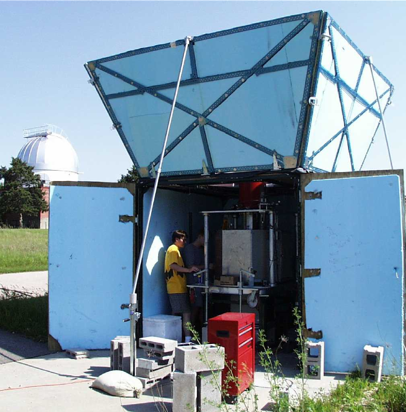
As mentioned in the previous chapter, polar is sensitive primarily to U, but as it rotates at $\sim$ 2 rpm, it can recover both Q and U. The polar receiver itself is a superheterodyne correlation polarimeter, and consists of three main parts: the cooled front-end, the room temperature back-end receiver and electronics, and post-detection electronics. A photograph of the instrument taken at the end of the 2000 observing season is shown in Figure 4.1.

4.1 The Front End

The front end of the receiver is shown schematically in figure Figure 4.2. The cold components reside in a cylindrical dewar . The dewar has both a 20K and 80K stage, and is cooled by a CTI-350 cold head in conjunction with an air-cooled, mechanical compressor. The dewar pressure was $1\cdot 10^{-6}$ torr for months at a time, and the cold head temperature was typically 22 K, although it was somewhat coupled with the ambient air temperature and in practice fluctuated between 21 and 23 K daily.

Figure 4.2: The polar dewar. The dewar is overly-large due to allowance for future receivers to be added at Q and W bands.

Figure 4.3: The polar vacuum window. The window consists of three layers: a 3-mil polypropylene layer to hold the vacuum, a layer of gore-tex for support against atmospheric pressure, and a layer of Volara above a dry nitrogen space to prevent water condensation on the window. Heater tape wrapped around the window kept the nitrogen space warm. The top window ring was also designed to accept the calibrator, which could be rotated above the dewar.

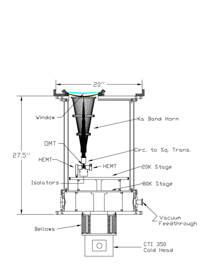
A brief summary of the signal chain is as follows: microwave signals pass through a virtually transparent vacuum window on the dewar face and into a cooled, corrugated microwave feedhorn. The signal is then split by an orthomode transducer (OMT), which separates the x- and y- components of the incident electric field. Both signals then pass through cryogenic, low-loss isolators and into HEMT amplifiers. After amplification, the joint signals travel out of the dewar and into the warm radiometer box, which houses the back-end microwave components. The signals are further amplified, mixed down to IF frequencies, multiplexed into three $K_{a}$ sub-bands, and finally correlated together. After the post-detection electronics, the signals are recorded to computer. Each of these steps will now be described in more detail.

4.1.1 The Vacuum Window

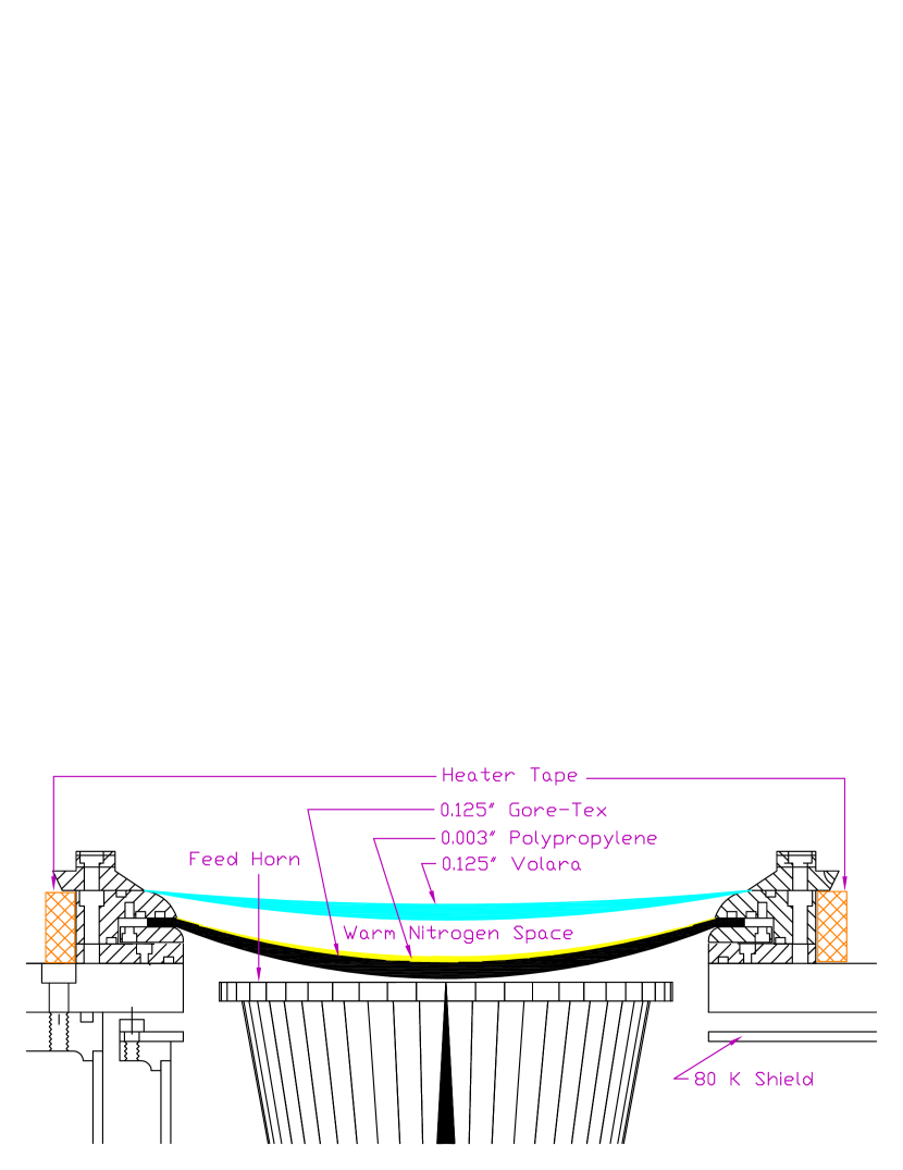
Our vacuum window is a true testament to human persistence. It evolved over a period of years, starting from the window design of the MSAM-II radiometer [103]. Initially, a 20-mil thick polypropylene window was used, as this had both the necessary strength and composition to hold the vacuum; however, it had some severe drawbacks. A minor drawback was the transmissivity of the window to infrared; as most of the IR got through, it increased the radiative loading on the dewar. More importantly, though, was the fact that the reflection coefficient is relatively high for a 20-mil layer of polypropylene, $\sim$ 10% for 30 GHz. For an anisotropy experiment only interested in intensity, this would not be a big problem, because the roughly 2 K reflected back into the dewar is fairly minor loading. For a polarization experiment however, this can be disastrous; a significant fraction of that reflected radiation can be polarized, leading to a large offset and much more stringent stability requirements.

Our team opted to avoid these potentially polarized offsets by constructing a window with an explicitly low reflection coefficient for microwaves. The vacuum window we arrived at is shown in Figure 4.3. The window holds vacuum using a 3-mil (0.003”) thick polypropylene window. This thin layer of plastic has a reflection coefficient of only $\sim$ 0.2% (compared with 10% for the 20-mil case). By itself, the thin polypropylene layer was not strong enough to hold against atmospheric pressure, and necessitated using a thin (1/8”) layer of Gore-Tex, which has the strength to hold the pressure across the 6.75”-diameter window (about 500 lbs). In addition, we found the Gore-Tex was almost completely opaque to infrared; this helped reduce the IR loading on the dewar, as the Gore-Tex layer was somewhat cooler than ambient air.

When this window was used in the field, significant condensation formed on the window, and proved an irksome issue throughout our campaign. The main defense against this condensation was use of a layer of Volara, which is an airtight, expanded polyethylene foam material. The Volara created a space which we filled with dry nitrogen and kept closed off from the ambient air. In the mornings, dew often condensed on the Volara, which was a separate problem. To combat this, heater tape was wrapped around the window structure; this kept the dry nitrogen (and hence the Volara layer) warm enough to usually hold off the dew. The loss of the entire window structure was found to be very low (emission less than 1 K).

4.1.2 Corrugated Feed Horn

After passing through the window, radiation enters our conical corrugated feedhorn. Our feedhorn was loosely based on the COBE 7^∘ corrugated feedhorn [104]. The recipe used to design the horn is given in Grant Wilson’s thesis [103], who himself used the classic book by Clarricoats and Olver [105] to design the feed, and the excellent paper by Zhang to design the wide-band mode launcher [106].

Figure 4.4: The measured beam patterns at 29 GHz for the polar corrugated feedhorn. The solid line is the E-plane copolar pattern, the dashed line is the H-plane copolar pattern, the dotted line is the E-plane cross-polarization pattern, and the dot-dashed line is the cross-polarization pattern measured at 45^∘to the E-plane. Note the close agreement of the E- and H-plane patterns, the low sidelobes of the copolar pattern, and the low level of cross-polarization in the main beam.

The measured beam pattern of the horn at 29 GHz is shown in Figure 4.4. Notice that the sidelobes are very low, near -70 dB at $\pm 90^{\circ}$ off-axis. Also, the cross-polarization response is quite low, better than -40 dB down from the main lobe response.

Of course, the beam pattern will vary with frequency, and this does not follow a strict 1/$\lambda$ behavior. We performed beam pattern measurements at 26, 29, and 36 GHz, but we would ideally like to know them at the polar sub-band center frequencies of 27.5, 30.5, and 34 GHz. Luckily, one can successfully model the beam response of a corrugated feed using a simple model that expands the electric field in Gauss-Laguerre modes [107].

Figure 4.5: Gauss-Laguerre and Gaussian beam models compared to measured beam patterns. The diamonds (26 GHz), triangles (29 GHz), and squares (36 GHz) are the measured beam patterns of the $K_{a}$ horn in the E-plane. The solid lines represent the corresponding Gauss-Laguerre approximations, while the dashed lines are the best-fit Gaussians to the main beam of the data. The Gauss-Laguerre theory involves no fitting – it has zero free parameters.

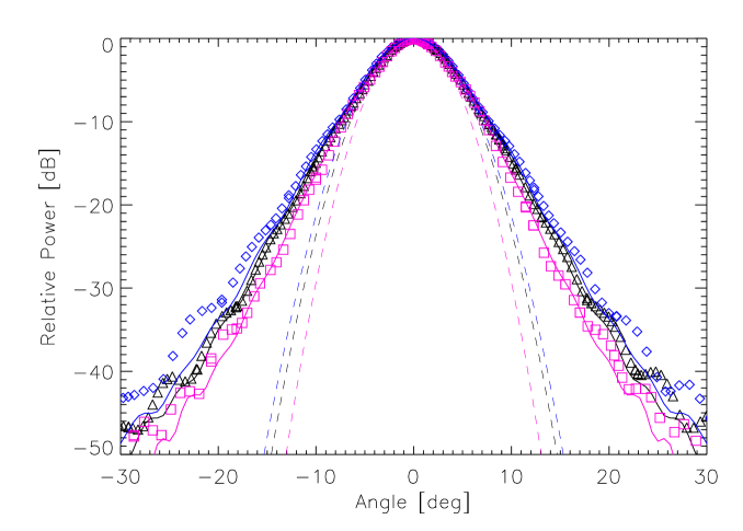
As shown in Figure 4.5, the Gauss-Laguerre model is an excellent approximation to the beam out to $\sim$ -40 dB. The beam pattern is Gaussian only over $\sim$ 1 FWHM, but later we will see that in the simplest data analysis, modelling our beam as a Gaussian is sufficient. Using this model, we can predict the approximate beamwidth at any frequency. The results for polar’s frequencies are shown in Table 4.2.

Frequency [GHz]	$\theta_{FWHM}\>\pm\>0.1^{\circ}$
27.5 (J3)	7.5∘
30.5 (J2)	7.0∘
34.0 (J1)	6.4∘

Table 4.2: Beam FWHM’s for polar’s three $K_{a}$ sub-bands, using Gauss-Laguerre theory.

The principle information to take away from the beam maps is that 1) we accurately measured the main beam response, including the FWHM’s in the Gaussian approximation, and 2) the sidelobes are very low, better than -50 dB at more than 35^∘ off-axis.

4.1.3 Cold Microwave Components: Isolators, OMT, HEMTs and Waveguides

The output signal from the corrugated feedhorn ends up in a circular $K_{a}$ band waveguide section, propagating the $TEM_{11}$ mode. This mode contains both x- and y-polarizations. Then the signal traverses a circular-to-square waveguide converter (maintaining both polarizations) and enters an Orthomode Transducer (OMT), which separates the x- and y- components of the incident electric field. The OMT is a critical component in our system, as our offset is directly based on how well the OMT does its job of completely separating the two polarization states; this effect was derived in §3.2.5. Graphs of some measured properties of our OMT are shown in Figure 4.6. No OMT is ever perfect, and we measured our OMT to have a roughly -30 dB cross-polarization (that is, roughly 0.1% of the power in the x-polarization state is transmitted to the y-output port, and vice-versa). Notice also that as much as 10% of the input power is reflected off the front port of the OMT; this effect serves to make our system less efficient, and can lead to standing waves through additional reflections from the window.

Figure 4.6: Measured OMT Properties. Solid lines correspond to the E-port properties, and dashed lines to the H-port properties. Isolation is symmetric between the two ports.

Both signals then pass through cryogenic, low-loss isolators and into HEMT amplifiers. The isolators had better than -22 dB isolation. The purpose of the isolators is to reject any backward propagating radiation that can lead to false signals, such as happens when some of the signal entering a HEMT is rejected off the input port and returns through the OMT, and then propagates down the other arm of the system. This renders the OMT isolation rather unimportant; OMT cross-polarization will be the dominant effect in offset generation.

The High Electron Mobility Transistor (HEMT) amplifiers were manufactured by Marion Pospieszalski at NRAO in 1994, and later retrofitted with low-noise, first stage Indium Phosphide (InP) transistors [108]. These gave them noise temperatures of $\sim$ 20 K. It is currently not possible to obtain lower noise amplifiers from any commercial vendor at these frequencies; they are truly “the most sensitive detectors in the world”.

Despite their amazing noise characteristics, the HEMTs are not perfect. As mentioned before, they reflect a non-negligible fraction of the incident power back towards the OMT, and necessitate the use of isolators. More importantly perhaps, their gain is not particularly flat; the roughly 25 dB of gain varies by as much as 5 dB across our nominal 10 GHz-wide band. These gain variations lower the effective bandwidth of the instrument, although the effect is partially compensated for by multiplexing into three sub-bands, as the sub-bands have much smaller relative gain variations than does the overall band; this effect is described in more detail in §4.2.3.

After this critical first stage of amplification the signals in each arm of the polarimeter (now averaging about $10^{-9}$ Watts) exit the dewar via a complicated, three-dimensional bending waveguide path, made of coin-silver waveguide. The last six inches of this waveguide are made of stainless steel, which provides the necessary thermal break between the cold and warm components of the system.

4.1.4 Dewar Temperature Observations and Control

The polar dewar had no system of temperature control, perhaps to the detriment of the experiment. We recorded temperatures at three points in the dewar using silicon diodes ; on the feedhorn, cold plate, and one HEMT body. These temperatures turned out to be quite coupled to the ambient air temperature; a 10^∘C change in air temperature resulted in an approximately 1^∘K change in temperature inside the dewar. A sample two-day period is shown in Figure 4.7; the coupling between HEMT and ambient temperature is quite striking.

Figure 4.7: Dewar and ambient (air) temperature changes over a two-day period. The dewar changed by about 1 K for every 10 K change in air temperature.

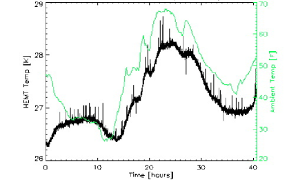
Thus, we are faced with a diurnal temperature variation of $\sim$3 K. Our signal was measured on the timescales of a single rotation ($\sim$ 30 sec). Over this timescale a believable HEMT temperature drift might be 10 mK. This could lead to a change in total power output by the HEMTs, but there is really no mechanism for this to lead to an apparent polarized signal, as the HEMT noises are uncorrelated.

4.2 The Back End

Figure 4.8: The polar signal chain.

4.2.1 RF Components

After leaving the dewar, the two signals traverse a section of copper waveguide and then pass into the Room-Temperature Radiometer Box (affectionately called the RadBox), which houses the warm radiometric components. Figure 4.8 shows the entire signal chain. First, the nanowatt signals are amplified again by commercial amplifiers of approximately 20 dB of gain, and $\sim$ 300 K noise temperatures. This may seem large, but the relative amount of noise added goes like one over the gain already experienced by the system, namely $\sim$25 dB in the cold HEMTs, so the relative noise added in this second stage of gain is a mere $300/10^{2.5}\;\sim\;1$ K.

4.2.2 Frequency Downconversion

The signals are then mixed down from RF (radiofrequency, 26-36 GHz) to IF (intermediate frequency, 2-12 GHz) via commercial mixers. The mixers are fed with a pure 38 GHz signal from a local oscillator (LO), which is subsequently split by a magic tee. One of these LO signals has a manually adjustable phase-shifter, so that one can tune the relative phase difference between the two LO signals, and thus between the resulting IF signals. The other LO signal contains an electronically-chopped phase switcher, which allows lock-in detection at the end of the signal chain; the phase switcher is square-wave chopped at 967 Hz, between 0^∘ and 180^∘(this was previously discussed in §3.1.5).

4.2.3 IF Amplification and Multiplexers

Following downconversion, the signals are further amplified by commercial IF amplifiers, and then split by commercial power splitters. One of each of these signals is then sent through a diode detector to monitor the total power level in that arm. These total power channels (referred to hereafter as TP0 and TP1) are very powerful monitors of atmospheric fluctuations, HEMT gain variations, and other systematic effects. Note that the TP signals are not chopped at the LO chop frequency, as their diode detectors are not phase sensitive.

The remainder of the split signals are themselves further amplified to approximately +12 dBm of power (approximately 15 mW), which will be required to fulfill the correlator power requirements. The signals are then multiplexed into the three $K_{a}$ sub-bands J1 (2–6 GHz), J2 (6–9 GHz), and J3 (9–12 GHz). The purpose of multiplexing is three-fold. First, one gains information on the frequency dependence of observed signals. Second, as we have no true filters, they are the primary band-defining element. The HEMTs and the feedhorn themselves have of course reasonably well-defined bands which minimize the pickup of out-of-band radiation, but the multiplexers ensure that no out-of-band signals propagate to the correlators. And finally, as alluded to before, the multiplexers serve to flatten the frequency response of the system, and hence increase the overall effective bandwidth. This is because effective bandwidth is given by [42]

$$\Delta\nu\;=\;\frac{\left(\int_{0}^{\infty}G(\nu)d\nu\right)^{2}}{\int_{0}^{\infty}|G(\nu)|^{2}d\nu}$$ (4.1)

Notice if $G(\nu)=1$ across a finite band (say from $f_{a}$ to $f_{b}$) and is zero elsewhere, then the effective bandwidth is $\Delta\nu=\frac{(f_{b}-f_{a})^{2}}{f_{b}-f_{a}}=f_{b}-f_{a}$, which is the maximum possible value. The more the band deviates from flatness, the smaller will be the effective bandwidth. The bandwidth measurements are discussed at the end of this chapter.

4.2.4 The Correlators

Once multiplexed, the six paths (three channels, two polarizations) pass through attenuators to bring them all to approximately 0 dBm of power (when looking at the sky). We found that the correlators needed at least -1 dBm of bias power into each arm to function properly, but more than +5 dBm caused them to saturate. This means that the total bias power can vary by only a factor of four and still ensure a linear response. Based on the radiometer equation, Equation (5.6), it is possible to see the maximum antenna temperature that the receiver can handle and still stay linear. If there is +0 dBm of power when looking at the $\sim$ 10 K sky, then the radiometer can accept at most 130 K of antenna temperature.

After this attenuation balancing act, each of the three channels in the “x” signal chain passes through a tunable IF phase adjuster before being correlated with its mate from the “y” signal chain. This is highly desirable, because if the two lines have picked up different phase shifts since they separated in the OMT, then their correlation will decrease (even if they were perfectly correlated to begin with), to a minimum of zero correlation if there was a 90^∘ relative phase shift between them. Finally, the two polarizations from each of the three channels are brought together in the correlators, which themselves are double-balanced mixers . The output from the correlators is DC, but only correlated input signals will produce an non-zero output. Because of the chopped phase in the LO signal, a correlated input signal to the polarimeter will produce, at the output of the correlators, a chopped signal at 967 Hz of $\pm V$, where $V$ is proportional to the correlated power of the two input polarization states.

4.2.5 Radbox Temperature Control

The fact that many of the components in the Radbox were temperature sensitive necessitated a robust system of temperature control. Without temperature control, gains from amplifiers, and power output by the mixers and LO would all drift due to their inherent temperature dependence, and add to the 1/f noise of the system. To minimize temperature drifts, all components inside the Radbox were heat sunk to a 0.25” aluminum plate. The plate itself was temperature-controlled via a standard PID circuit. The PID circuit keyed off a temperature sensor mounted directly to the local oscillator, which we found to be the most critical component in terms of temperature dependence. The PID circuit controlled the temperature via heaterfoil pads mounted underneath the aluminum plate. We found the temperature inside the RadBox to be stable to $\sim$ 100 mK per day.

4.3 Post-Detection Electronics and Data Acquisition

Five channels thus leave the radiometer box: the two total power channels, TP0 and TP1, corresponding to the power in the x- and y- polarizations of the signal, and the three correlator channels labelled J1, J2, and J3. In voltage units, all these signals are small (a few $\mu V$ for the correlators), and are further amplified by a home-made differential pre-amplification circuit.

The correlator channels then pass into a lock-in amplifier that correlates the channels with the square-wave reference signal feeding the LO phase chopper. They are also correlated with a “quadrature-phase” signal, which is the input chop signal shifted in phase by 90^∘. This results in six correlator signals, three from the in-phase correlation and three from the quadrature-phase correlation. The quadrature-phase channels (hereafter QPC) are not sensitive to signal and thus serve as a powerful check of systematics and problems with the electronics.

Following lock-in detection, all channels pass through 5 Hz, 24 dB/octave low-pass filters to prevent aliasing. These eight signals are then recorded at 20 Hz via a Labview-controlled, National Instruments data acquisition system running on a Windows-98 laptop, mounted inside the rotation stage. Finally, data files were written every 7.5 minutes over an ethernet connection to a remote computer, where they awaited later analysis.

Data Channels
Channel	Description
TP0	Total Power Channel 0 (HEMT A31), “$I_{x}$”
TP1	Total Power Channel 1 (HEMT A32), “$I_{y}$”
J1i	In-Phase Correlator Channel, 32-36 GHz
J2i	In-Phase Correlator Channel, 29-32 GHz
J3i	In-Phase Correlator Channel, 26-29 GHz
J1o	Quad-Phase Correlator Channel, 32-36 GHz
J2o	Quad-Phase Correlator Channel, 29-32 GHz
J3o	Quad-Phase Correlator Channel, 26-29 GHz
House-Keeping Channels
$T_{cp}$	Temperature of Cold Plate (typ. 24 K)
$T_{hemt}$	Temperature of HEMTs (typ. 27 K)
$T_{horn}$1	Temperature of Horn (typ. 40 K)
$T_{LO}$	Temperature of Local Oscillator (typ. 39∘ C)
AOE	Absolute One-Bit Encoder
Encoder2	16-Bit Relative Encoder
Radmon	Current monitor for RadBox Temperature Control Unit
Octomon	Current monitor for Octagon Temperature Control Unit

Table 4.3: Data Acquisition Channels for polar.

• Failed very early in season.

• Failed after approximately one month of data taking.

In addition to the eight primary signal channels, the data acquisition system was capable of recording eight addition channels of data (all were in non-referenced, single-ended mode). Table 4.3 provides a list of all channels and their descriptions. These included three temperature sensors in the dewar, one temperature sensor in the radiometer box, the AOE and encoder signals (described below), and the current being used by the two temperature control units.

4.3.1 A Note on the Lock-In Technique

As stated previously, the primary advantage of phase chopping the signal and subsequent lock-in detection is to drastically reduce 1/f noise, due primarily to gain fluctuations in the HEMTs. However, one might naively assume that there is a price associated with phase chopping, but this is not so. Because we are chopping from 0^∘ to 180^∘, a correlated signal will be chopped between some $\pm V$, where V is proportional to the level of polarization in the signal. As we are square-wave chopping, no integration time is actually lost, and thus our sensitivity is not degraded by any factor of $\sqrt{2}\;$ as might be expected. This would not be the case if we were sine-wave chopping, where some integration time is lost, and one would lose a factor of $\sqrt{2}\;$ in that case.

4.4 POLAR Housing and Rotation Mount

Figure 4.9: Schematic of polar inside the cubical plywood housing.

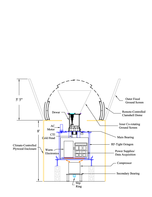
4.4.1 The POLAR cube

Figure 4.9 shows the polar instrument inside its housing. polar lived at the Pine Bluff Observatory in Pine Bluff, WI, inside a small housing built of plywood and unistrut, insulated with 2-inch thick styrofoam. This enclosure was temperature controlled by a heater/air conditioner system which kept the cube temperature at roughly 60^∘F, although this temperature varied somewhat over the course of the season, where the outside temperature ranged from 10^∘F to 85^∘F.

polar was guarded against the elements by a small fiberglass clamshell dome made by AstroHaven Inc. It used AC motors to control the opening and closing of the dome. During inclement weather, the dome could be closed either locally using a small control pad, or remotely via an Internet interface on a private web page.

4.4.2 Weather Station

A small commercial weather station was mounted on the control building near the polar cube. This station measured outside temperature, wind speed and direction, and humidity, every five seconds. This data was recorded in our time stream every 7.5 minutes.

4.4.3 Rotation Mount and AOE

polar’s rotation was driven by an AC motor, connected to a large concentric gear at the base of the dewar. The aluminum gear plate sat on a groove filled with stainless steel bearings; we found the rotation to be quite smooth. The rotation was also robust; polar underwent approximately 120,000 rotations in the 2000 observing season with almost no problems The rotation rate was measured to be $0.0332\ \pm\ 0.0003\ Hz$.

At the beginning of the season, we recorded the angular position of polar with a relative 12-bit encoder. To make it absolute, we constructed an “Absolute One-Bit Encoder” (hereafter AOE). This simple optical device was mounted on the rotation stage, and output a short voltage pulse whenever a certain point on the non-rotating stage was passed. The AOE contained an opto-coupler that output 5 volts whenever a reflective surface was close to its sensor (within $\sim$ 0.5”). At due north on the non-rotating stage was mounted a small piece of absorptive tape, so the signal from the AOE dropped to zero volts whenever the rotating stage passed due north. This simple system, coupled with the smooth rotation of polar, obviated the need for a more accurate encoder, which was ultimately abandoned when it failed in the field.

A brief note on POLAR’s coordinate system

polar’s coordinate system is defined in actuality by the OMT/circular-square transition; everything above this point is axially symmetric. It should be noted that the axis of symmetry defined by this coordinate system was not aligned with local North-South when the AOE pulse occurred. However, we measured this angle to be $23^{\circ}\pm 1^{\circ}$ at the end of the observing season. This measurement ultimately enables presentation of results in the standard IAU system (see, for example, reference [49]).

4.4.4 The Octagon

The warm radiometer box was mounted inside an RF-tight cage that co-rotated with the dewar. This cage, called the “octagon” (due to its octagonal shape), housed power supplies, the HEMT bias cards, temperature control circuits, and the data acquisition system, in addition to the Radbox. It was temperature controlled via a similar circuit as for the Radbox (§4.2.5), except with much larger heater pads. The octagon was typically kept at 28^∘C, and varied by less than 0.5^∘C per day. This temperature control also made life easier for the temperature control circuit inside the Radbox; as the air external to the Radbox was at a fairly stable temperature, the intrinsic temperature variations inside the Radbox were minimized, so only a small amount of power was necessary to temperature stabilize the Radbox internal components.

4.4.5 Compressor and Slip Ring

Beneath the RF cage sat the cryocooler compressor, which also rotated with the rest of the system but on a separate bearing. Underneath the compressor sat an 8-line slip ring, through which data and power were transferred between the fixed and rotating stages. Four lines were used for the $\sim$ 2 kW of power that polar required for operation, and two lines were used for data. The data stream was sent from the rotating laptop through the slip ring to an ethernet cable, to the computer in a nearby control room which recorded the data.

4.4.6 Ground Screens and Spritz Tests

Although the sidelobe response of our feedhorn was very good, we sought further sidelobe rejection through the use of two sets of ground screens. The inner ground screen was purely conical, and was mounted to the top surface of the dewar. In order to minimize possible polarized reflections, we coated this aluminum surface with Eccosorb; with the opening angle of 26^∘ of this shield, it should introduce less than 30 mK of unpolarized antenna temperature to our system. Even if it is slightly polarized, it’s immaterial as this shield co-rotated with the dewar, and thus would not be modulated like a true sky signal.

In addition to the inner ground screen, we built a non-rotating, scoop-type outer ground screen, composed of four large, trapezoidal aluminum panels. In times of high winds, these panels were easily lowered to the sides of the cube via hinges. A simple scalar diffraction calculation estimates an extra 40 dB of sidelobe rejection from this ground screen; including the feed horns gives an estimate of better than 100 dB of sidelobe rejection from the 300 K earth. However, we discovered that the true rejection of side lobes was not nearly as good.

Figure 4.10: Side view of the Spritz test set-up. A double refraction is generally necessary for signals deep in the side lobes to be detected by the system.

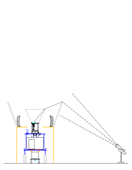
“Spritz tests” enable one to trace out the side lobes of a telescope, by using a small, hand-held microwave source. The source is moved to different places in the side lobes, and the system response is monitored. As shown in Figure 4.10, a double refraction is in principle required for the signal to reach the feedhorn. We conducted a series of these tests at the end of the 2000 observing season , and discovered that the signal was attenuated only by $\sim$ -50 dB when placed further than 90^∘ into the sidelobes. However, the signal was generally largest when aimed directly at the cube housing, meaning that somehow the signal was getting into the system from within the cube, although it is difficult to construct a mechanism for this. In retrospect, we should have coated the plywood cube (plywood is of course transparent to microwaves) with something reflective to prevent such paths into the system.

Although this situation is definitely undesirable, it is not perhaps as terrible as it seems: the 300 K earth is probably less than 1% polarized, leading to a $\sim 30\mu K$ earth-based signal, modulated at the rotation frequency. This is not consistent with true polarized sky signals, which are modulated at twice the rotation frequency; only the first harmonic would survive the lock-in to twice the rotation frequency, which should be significantly less than 30 $\mu K$. However, this is still an important systematic which may haunt us later in Chapter 8.

4.5 Basic Radiometer Performance: Bandpasses and Power Spectra

Now that the structure of the radiometer has been described, let us discuss somewhat how well it worked. In the lab, we attempted to characterize the calibration, noise figures, bandwidths of the radiometer. We delay the discussion of calibration and system temperature until Chapter 5.

4.5.1 Bandpass

We never performed a full bandpass measurement on the system, but we did do a test of the bandpass for the warm radiometer box. These tests did not include the cold radiometric components, such as the HEMTs and OMT. A 26-36 GHz signal was generated with an RF sweeper. This signal was attenuated by about 50 dB to compensate for the $\sim$ 60 dB of gain of the Radbox, and subsequently split with a magic tee into two equal pieces. These components were fed into the two Radbox input ports, and we subsequently measured the output from each correlator channel (after lock-in). Because the signals came from the same source, they were perfectly correlated. The resulting bandpasses are shown in Figure 4.11.

Figure 4.11: Bandpasses through the radiometer box for the three in-phase (IPC) correlator channels. From left to right, the channels are J3, J2, and J1. The upper curves represent the bandpasses when the chopped phase shifter is the 0^∘ (+) state, whereas the lower curves correspond to the 180^∘ (-) state. Also shown are the effective bandwidths of each sub-band in the Radbox, calculated using Equation (4.1). This leads to a total effective bandwidth of about 9.5 GHz for the Radbox, but this does not include the HEMT amplifiers or any other dewar or optical components.

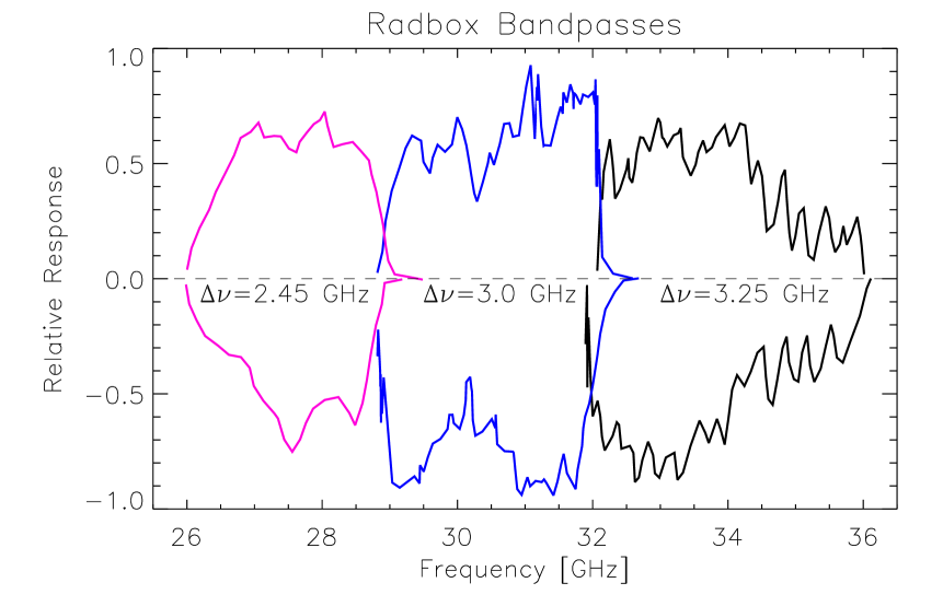
The bandpasses shown in the figure are quite acceptable. Since the measurements did not include the cold radiometer components, we cannot take this as the true bandpass of the system, but these measurements are suggestive of the generally good performance of the components we employed.

4.5.2 Power Spectra

Figure 4.12: Sample power spectra from the polar radiometer, in noise equivalent temperature (NET) units. These spectra were taken under good weather conditions, while observing the zenith. The total power channels display their characteristic 1/f noise, which is noticeably absent in the three correlator channels. Also seen is the effect above a few Hz of the anti-aliasing filters. The vertical dashed lines correspond to once and twice the instrument rotation frequency (labelled $1\phi$ and $2\phi$); polarization signals induce a spike at the $2\phi$ frequency.

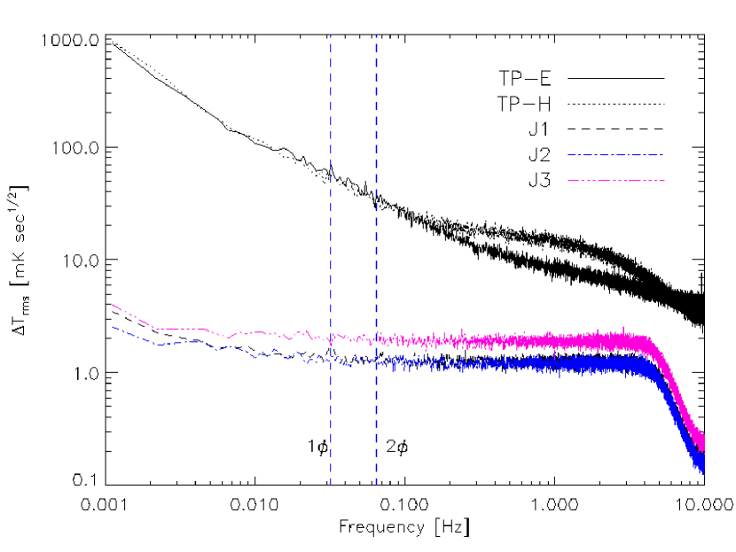
Some sample power spectra for the system are displayed in Figure 4.12. These were taken outside, under good weather conditions while staring at the zenith. Notice how flat the low-frequency power spectra are for the correlator channels; this is quite good, and is a testament to the power of both the correlation radiometer, and the phase-switching lock-in technique. The power spectra from the total power channels are also shown, and they display the characteristic “1/f noise” intrinsic to the HEMT amplifiers. At the frequency of interest where polarization signals can be seen (namely twice the polar rotation frequency), the total power channels are roughly thirty times less sensitive than the correlator channels! Note also the presence of the 5-Hz low-pass, anti-aliasing filters in all of the channels.

In this chapter, we have seen that the polar instrument is indeed a stable, sensitive polarimeter, capable of viewing both Stokes $Q$ and $U$ parameters, and hopefully finding the CMB polarization. However, before observations can begin, we must complete the final instrumental task, calibration of the instrument. This non-trivial task is described in detail in the next chapter.

Chapter 5 Calibration

5.1 Background

Calibration is an ever-present challenge to all CMB experiments. However, a typical CMB anisotropy experiment requires calibration only in the sense of total power; that is, phase information is irrelevant, and of the four Stokes parameters, only I is important. This is not the case with a polarization-sensitive receiver. In that case, one should calibrate all the Stokes parameters that one plans to measure.

In addition to determining the calibration proportionality constants (that is, the voltage one expects for a given signal strength in Kelvins) for each Stokes parameter, the system calibration also serves to tell us about the noise characteristics of our system. Specifically, we would like to know how each of the following quantities changes over time:

• $T_{rec}$ – The equivalent antenna temperature due to the noise of the radiometer itself.

• $T_{sky}$ – The antenna temperature input to the radiometer (a sum of radiation from the sky, atmosphere, and CMB).

• $\Delta\nu$ – The RF bandwidth of each radiometer channel.

• $NET$ – The “noise equivalent temperature” of the system, in $mK\sqrt{s}$, which tells how long it takes to integrate to given signal level.

• System offsets for each channel.

• Cross-talk between channels.

Ideally, we would not only measure these quantities accurately, but we would measure them often, to understand how our system changes with time. This chapter describes how (and how well) this was done for polar.

5.2 Radiometry Basics

Before going any further, it will be useful to lay out some of the basics of microwave radiometry, as these techniques and formulas are most useful in understanding the calibration and assessing the noise of the instrument. These are only the absolute basics; for a more detailed review of this material, some excellent sources are [109, 110, 42].

5.2.1 Temperature in Radio Astronomy

To understand radiometry, we must know the units of radiometry, which confusingly include no fewer than three different types of temperature (in addition to many other quantities)! The brightness temperature of a source as a function of frequency is a way of characterizing the power emitted by it at a certain frequency, and is given by

$$T_{B}(\nu)\equiv\frac{\lambda^{2}B(\nu)}{2k_{B}}$$ (5.1)

where $k_{B}$ is Boltzmann’s constant, and $B(\nu)$ is the blackbody emission spectrum, given by

$$B_{\nu}=\frac{2h\nu^{3}}{c^{2}}\frac{1}{e^{h\nu/kT}-1}\;\;\;\;\;[Wm^{-2}Hz^{-1}sr^{-1}]\;\;\;\text{;}$$ (5.2)

note that brightness temperature is only the same as thermodynamic temperature when in the Rayleigh–Jeans limit of $h\nu\ll k_{B}T$.

However, radio telescopes measure a quantity called antenna temperature, which itself depends on the beam pattern of the telescope, while brightness temperature is a function of the source only. In the special case that the source completely fills the beam, the antenna temperature equals the object brightness temperature. Otherwise, a brightness distribution $T_{B}(\theta,\phi)$, when measured by a system with a normalized beam power response of $G(\theta,\phi)$, viewing in a direction $(\theta_{0},\phi_{0})$ yields an antenna temperature of

$$T_{ant}=\int_{4\pi}T_{B}(\theta,\phi)G(\theta-\theta_{0},\phi-\phi_{0})d\Omega$$ (5.3)

which is just the convolution of the source brightness distribution with the beam pattern.

Thermodynamic temperature is the quantity typically reported; based on Equation (5.1), we can see these quantities are related by

$$T=T_{ant}\frac{e^{x}-1}{x}$$ (5.4)

where $x\equiv\frac{h\nu}{k_{B}T}$. In typical anisotropy experiments, we measure not absolute temperatures, but rather temperature differences. In polarization measurements it is the same; recall for instance that $Q=I_{x}-I_{y}$. That is, polarization temperatures are really temperature differences, hence the same temperature relationships hold for polarization as for temperature anisotropy, and by differentiating Equation (5.4), one arrives at

$$\Delta T=\Delta T_{ant}\frac{(e^{x}-1)^{2}}{x^{2}e^{x}}$$ (5.5)

For the $K_{a}$ band, this factor is about 1.025. Unless otherwise noted, all temperatures in this work will be reported in units of thermodynamic temperature.

5.2.2 The Radiometer Equation

By far, the most important formula in radiometry is known as the “Radiometer Equation” [42], which relates the smallest detectable signal to the properties of the radiometer:

$$\Delta T\;=\;\kappa\frac{T_{rec}+T_{load}}{\sqrt{\Delta\nu\;\tau}}$$ (5.6)

where

$\Delta T$ is defined as the smallest possible signal that can be detected at the 1-$\sigma$ level with the system in question.

$T_{rec}$ and $T_{load}$ are both antenna temperatures. $T_{rec}$ is the equivalent antenna temperature due to the noise of the radiometer itself, and $T_{load}$ is the antenna temperature as seen by the feedhorn (not including our window or other auxiliary optics).

$\Delta\nu$ is the RF bandwidth of the radiometer, and is given by Equation (4.1). Note that it depends only on the shape of the bandpass; the flatter, the better.

$\tau$ is the integration time.

$\kappa$ is a constant of order unity that is associated with the type of radiometer being used. For correlation radiometers like polar, $\kappa=\sqrt{2}$.

Equation (5.6) can be ’compactified’ by defining the Noise Equivalent Temperature (NET) of the system, which is the temperature limit obtained after one second of integration:

$$NET\;=\;\kappa\frac{T_{rec}+T_{load}}{\sqrt{\Delta\nu}}\;\;\;\;[K\;s^{-1}]$$ (5.7)

Then the radiometer equation becomes simply $\Delta T={NET}/{\sqrt{\tau}}$. The Noise Equivalent Voltage (NEV) is the uncalibrated version of the NET. It is measured in $V\cdot\sqrt{s}$, and is the voltage limit obtained after one second of integration. Equation (5.7) is only approximately correct for a correlation polarimeter. A more correct expression takes into account the fact that the two different arms of the polarimeter can have different receiver temperatures (as they contribute potentially different amounts of noise to the system). Then the NET becomes

$$NET\;=\;\kappa\sqrt{\frac{(T^{L}_{rec}+T_{load})(T^{R}_{rec}+T_{load})}{\Delta\nu}}$$ (5.8)

where $T^{L,R}_{rec}$ are the receiver temperatures for the two polarimeter arms. Even though this equation appears quite non-linear, it is deceptive; if the two receiver temperatures are fairly close, then the NET is approximately

$$NET\;\simeq\;\kappa\frac{(\sqrt{T^{L}_{rec}T^{R}_{rec}}+T_{load})}{\Delta\nu}\qquad.$$ (5.9)

5.2.3 System Response and Y-factor

The general voltage response of our radiometer to an input antenna temperature $T$ is given by

$$\texttt{{v}}=k(T_{rec}+T_{load})+\texttt{{v}}_{0}$$ (5.10)

where k is the calibration coefficient, and $\texttt{{v}}_{0}$ is the offset due to the post-detection electronics (such as a pre-amplifier offset), and is assumed to be known. Here, v represents only our total power channels. If v is a correlator channel, then we keep only the polarized fraction of $T_{rec}+T_{load}$. Notice that v is linear in the input temperature; this may surprise those who recall that the total power emitted by a blackbody goes roughly like $T^{4}$. The problem is solved when we realize that the power collected by our radiometer is

$$P\;=\;k_{B}T\Delta\nu$$ (5.11)

if we are in the Rayleigh-Jeans part of the emitting object’s spectrum. This is a simple consequence of integrating the Planck distribution under the approximation $h\nu\ll k_{B}T$. For a single-mode receiver and a single polarization,

$$P\ =\ \int_{\nu_{1}}^{\nu_{2}}\frac{h\nu}{e^{h\nu/k_{B}T}-1}d\nu\simeq\int_{\nu_{1}}^{\nu_{2}}k_{B}Td\nu\ =\ k_{B}T\Delta\nu\ .$$ (5.12)

As the radiometer response is linear in the power collected, we see it is also linear in the antenna temperature.

A “y-factor” measurement is a simple technique to determine the calibration coefficient $k$ as well as $T_{rec}$ from measurements of the system response to two known temperatures, say $T_{1}$ and $T_{2}$ (typically 77K and room temperature). If these yield responses of $\texttt{{v}}_{1}$ and $\texttt{{v}}_{2}$, respectively, then

$$k\;= \;\;\;\;\;\;\;\;\;\;\;\frac{\texttt{{v}}_{2}-\texttt{{v}}_{1}}{T_{2}-T_{1}}$$ (5.13a)

$$T_{rec}\;= \;\;\;\frac{T_{2}(V_{1}-V_{0})-T_{1}(V_{2}-V_{0})}{V_{2}-V_{1}}$$ (5.13b)

However, this simple technique only works for total power channels; channels responsive to a polarized signal must be calibrated by varying a polarized input signal, and tracking the system response. Simply varying the power in an input unpolarized signal will only vary the noise in the channel; it will not (in principle) generate a signal response. The subject of calibrating a polarization channel is treated in §5.3.

5.2.4 Noise Response and Y-factor

The signal is not the end of the story, however. As a senior graduate student told me as I began to work on this project, “Our signal is noise.” While this was not quite true, understanding one’s noise is of critical importance.

It is assumed the reader is familiar with the basics of auto-correlation, cross-correlation, and the Power Spectral Density (PSD). If not, an excellent introduction for experimentalists is given in Numerical Recipes, reference [111]. All channels have a power spectral density, or PSD, measured in $V^{2}/Hz$ that is proportional to the system temperature squared (where for correlators we use the approximation of given in Equation (5.9), where the receiver temperature is taken to be the geometric mean of the two arms’ receiver temperatures). A more convenient quantity is the PSD amplitude, which is simply the square root of the PSD, and has units of $V/\sqrt{Hz}$.

We measured the PSD amplitude of the system several times in the lab before the instrument was deployed, and then several times during the season (see Figure 4.12). For the correlator channels, this provides the means to determine their receiver temperatures. Imagine we view a sky temperature $T_{1}$ and a second temperature $T_{2}$ , then use the following algorithm:

1. Record several minutes of data for each load condition.

2. For a given channel, compute the power spectral densities $P_{1}(\nu)$ and $P_{2}(\nu)$ under the two load conditions.

3. Where the PSD is flat, or at the signal frequency, evaluate each PSD. Multiplying by $\sqrt{2}$ will yield the NEVs, $\eta_{1}$ and $\eta_{2}$, under each load condition .

4. The receiver temperature in that channel is then given by

   $$T_{rec}\;=\;\frac{T_{2}\eta_{1}-T_{1}\eta_{2}}{\eta_{2}-\eta_{1}}$$ (5.14)

Once we know the calibration coefficient of a given channel, we can calculate the NET of that channel by multiplying the NEV by the calibration coefficient. At this point, we can calculate our channel bandwidth $\Delta\nu$ by using Equation (5.6). If $\Delta\nu$ is known by other means (such as by direct measurement of the bandpass and then using Equation (4.1)), then other quantities in Equation (5.6) can be verified.

5.3 The POLAR Calibration

The following section was originally published as a separate paper, see [112].

At this point, we must determine a method with which to calibrate our polarization channels. In general, there are three types of calibration we could appeal to: internal, external (local), and astrophysical. For internal-type calibrations, some type of noise source, mounted within the front-end, is used to inject a known signal into the radiometer. However, to make a well-understood polarized signal requires an additional OMT, and this was not within our budget. Astrophysical calibration is perhaps the easiest; by pointing the radiometer at sources of known flux (at your particular frequency), calibration is achieved by comparing the response to the known flux. To determine the effectiveness of a point source calibration, first we must compute our sensitivity to point sources, given by the Rayleigh-Jeans relation [42]; for a Gaussian beam, this relation is

$$\frac{T(\nu)}{S(\nu)}=1.053\;\frac{\lambda^{2}}{\theta^{2}_{1/2}}\;\;\;\;[K/Jy]$$ (5.15)

where $S(\nu)$ is the flux density of the point source in Jy, $\lambda$ is in meters, and $\theta_{1/2}$ is the beam FWHM in degrees. For polar’s 7^∘ beamsize, this works out to only 2 $\mu K$/J, which is more than an order of magnitude too small to calibrate from even the most powerful radio sources [102].

Thus, we abandon both internal and astrophysical calibration techniques; instead, we must rely on some type of external approach. The standard way to generate a known polarized external signal is by placing a wire grid above the radiometer at a 45^∘ angle to the antenna axis[31, 113]. Wire grids are simple, reliable, and have well-understood properties [114, 115, 116, 117]. If a hot load of temperature $T_{H}$ is placed to the side (such that it will reflect in one polarization), and a cold load of temperature $T_{C}$ is placed above the grid, both in such a way that they completely fill the beam, the radiometer will receive a polarized signal of temperature $T_{H}-T_{C}$. Using liquid nitrogen for the cold source results in a $\sim$ 200 K polarized signal. This is troublesome for two reasons. First, this signal is $\sim$ 8 orders of magnitude larger than the signal we are actually trying to measure; indeed, the signal reaching the correlators will be almost 100% correlated (provided the radiometer is rotated to the appropriate angle). Second, and perhaps more important, we remember that our calibrators can only handle $\sim$ 90 K of antenna temperature before compressing. Clearly, we need a smaller polarized signal, and ideally one that is only very slightly polarized, to more closely mimic the tiny CMB signal that we seek.

Recently, Hedman et al. [40] used reflection of a known (unpolarized) source from a metal surface to create a well-characterized but small polarization signal for their calibration[118]. For polar, we used yet another approach – reflection of thermal radiation from a thin dielectric sheet. The rest of this section will describe what we learned in trying to perform and understand this calibration technique; in order to make the technique useful to as wide as possible an audience, the discussion is kept relatively general.

5.3.1 The Technique

In order to calibrate polar, we replaced the wire grid in the conventional set-up with a thin dielectric sheet (see Figure 5.1). The sheet’s composition and thickness were chosen carefully according to criteria discussed later in this section. If the reflection and emission properties of the sheet can be ascertained, through either direct measurement or calculation, then it is straightforward to calculate the expected signal from the dielectric. Both the hot and cold loads emit blackbody radiation at their physical temperatures, $T_{H}$ and $T_{C}$ respectively. These unpolarized sources emit an equal amount of radiation polarized both perpendicular (TE) and parallel (TM) to the plane of incidence on the dielectric sheet. Note that the TE and TM radiation fields are uncorrelated with each other. Upon traversal of the sheet, a certain amount of each of these four fields arrive at the aperture of the polarimeter, along with the oblique emission from the sheet itself (which has a physical temperature $T_{S}$).

Figure 5.1: Calibration Set-Up using the thin dielectric sheet. Unpolarized radiation from both a hot load (side) and cold load (top) is partially polarized due to the slight difference in $R_{TE}$ and $R_{TM}$ of the sheet, thus causing the polarimeter to see a slightly polarized signal. The angle between the polarimeter $x$-axis and sheet plane of incidence is $\phi$. The Stokes parameters can be modulated by variation of the angle $\phi$.

In order to perform the calibration, we must determine the intensity of fields at the aperture of the polarimeter from the calibrator. We use the standard Stokes parameters $\{I,Q,U,V\}$ to characterize field intensity. The Stokes parameters are additive quantities and hence simplify the following mathematics.

In [113], the Stokes parameters from a wire grid calibrator are calculated. For the dielectric sheet the derivation is similar, but we must also take into account the emissivity of the sheet, which may not be negligible. We will make the simplifying assumption that the microwave absorbers ($T_{C}$ and $T_{H}$) are perfect blackbodies; this assumption will be discussed later in detail.

First let us calculate the Stokes parameters in the reference frame of the calibrator; once we have these, it is straightforward to “rotate” them into the frame of the polarimeter. We give the Stokes parameters in units of brightness temperature; for a single-mode antenna in the Rayleigh-Jeans limit, the brightness temperature $T_{B}$ is related to power $P$ through $P=\Delta\nu k_{B}T_{B}$, where $\Delta\nu$ is the frequency bandwidth and $k_{B}$ is Boltzmann‘s constant. Let $\hat{x}$-$\hat{y}$ be the coordinate system of the calibrator, and $\hat{x}^{\prime}$-$\hat{y}^{\prime}$ be the coordinate system of the polarimeter; $\phi$ denotes the rotation angle between these reference frames. Further, let $I_{x}$ and $I_{y}$ correspond to the brightness temperature of the total power polarized along $\hat{x}$ and $\hat{y}$, respectively. The Q Stokes parameter is given by $Q=I_{x}-I_{y}$. The brightness temperatures $I_{x}$, $I_{y}$, $Q$, and $U$ in the (unprimed) calibrator coordinate system will be (see Appendix A):

$$I_{x} = T_{C}+\left(T_{H}-T_{C}\right)R_{TE}+\left(T_{S}-T_{C}\right)\epsilon_{TE}$$ (5.16a)

$$I_{y} = T_{C}+\left(T_{H}-T_{C}\right)R_{TM}+\left(T_{S}-T_{C}\right)\epsilon_{TM}$$ (5.16b)

$$Q = \left(T_{H}-T_{C}\right)\left(R_{TE}-R_{TM}\right)$$ (5.16c)

$$+\left(T_{S}-T_{C}\right)\left(\epsilon_{TE}-\epsilon_{TM}\right)$$

$$U = 0$$ (5.16d)

If the angle between the polarimeter $\hat{x^{\prime}}$-axis and the sheet plane of incidence ($\hat{x}$-axis) is $\phi$, then the Stokes parameters as seen by the polarimeter are given by

$$I_{x^{\prime}} = I_{x}\cos^{2}{\phi}+I_{y}\sin^{2}{\phi}$$ (5.17a)

$$I_{y^{\prime}} = I_{x}\sin^{2}{\phi}+I_{y}\cos^{2}{\phi}$$ (5.17b)

$$Q^{\prime} = Q\cos{2\phi}$$ (5.17c)

$$U^{\prime} = -Q\sin{2\phi}.$$ (5.17d)

We note here that including the small reflectance $R_{l}$ of the unpolarized loads would have the effect of increasing $T_{C}$ to $T_{C}+R_{l}(T_{H}-T_{C})$ in the reflection term in Equation (5.16), assuming the environment has a temperature $T_{H}$. Typically the loads can be chosen such that the overall effect can be neglected. If this is not possible, $R_{l}$ must be measured at the frequencies of interest, so that its effect on Equation (5.16) can be included.

It is then a simple matter to calibrate the polarimeter by varying the angle $\phi$, either by rotating the calibrator or the polarimeter. As we are primarily interested in calibrating polarization channels, we will focus on the $Q$- and $U$-calibration signals; each of these changes by a full 100% over a complete $\phi$ cycle. In contrast, varying $\phi$ produced very low signal-to-noise variations in $I_{x^{\prime}}$ and $I_{y^{\prime}}$ for the dielectric sheets we used, making a “total power” calibration with the sheet impractical. However, this is inconsequential because those channels are easily calibrated with simple unpolarized loads through a conventional y-factor measurement.

The accuracy of the $Q$- or $U$-calibration depends on several factors. First, one must know or determine the relevant material properties of the sheet, namely the reflection coefficient and emissivity both for the two polarization states and as a function of incidence angle. The angle of incidence $\theta$ must be known to reasonable accuracy. The sidelobes of the receiving horn should be low, the sheet and loads should be large enough to completely fill the main beam of the receiver, and the loads should be near-perfect absorbers, else stray radiation from the surroundings will enter the system. All these conditions must be satisfied in the wire grid approach as well, with the exception that instead of understanding the grid properties, now it is the reflection and emission properties of the dielectric sheet that we seek to understand. It is on these issues that we will now focus.

5.4 Dielectric Reflection and Emission Properties

The general situation we wish to consider is as follows: an electromagnetic wave of wavelength $\lambda$ is incident upon an infinite dielectric sheet of thickness $d$ and index of refraction $n$. Part of this wave will be reflected, part will be transmitted, and part will be absorbed. All these quantities will depend upon the polarization state of the incident wave, which in general will be a combination of $TE$- and $TM$-polarized radiation. Thus, for the radiation incident upon the sheet (to be distinguished from its own thermal emission), we have

$$|r|^{2}+|t|^{2}+A\ =\ 1$$ (5.18)

where $|r|^{2}$, $|t|^{2}$, and $A$ represent the fractional power reflected, transmitted, and absorbed, respectively; $r$ and $t$ are the usual Fresnel reflection and transmission coefficients, and are complex quantities.

If the sheet is in thermal equilibrium, emission will equal absorption (i.e., $\epsilon=A$). In general, a material has a complex index of refraction $N=n-j\kappa$ where $n$ corresponds to the real index of refraction, and $\kappa$ is the extinction coefficient and determines the loss of the material. If $\kappa\ll n$, then the loss tangent of the material, the ratio of the imaginary component to the real component of the dielectric constant, is given approximately by

$$\tan{\delta}\approx\frac{2\kappa}{n}\ .$$ (5.19)

Given N, it is possible to calculate both $r$ and $t$ for a lossy dielectric slab [98]. Then the emissivity $\epsilon$ will be $1-|r|^{2}-|t|^{2}$, and in general will be polarized. However, for this treatment we assume that the total loss in the dielectric is negligible; §5.4.2 deals with the conditions under which this assumption is valid.

5.4.1 The Reflection Term - Theory

It is straightforward to derive the reflection coefficients for our smooth dielectric sheet using the Fresnel equations, under the assumptions that the dielectric is homogeneous, optically isotropic, non-amplifying, and the wavelength is on the order of or larger than the film thickness, such that all the multiply-reflected beams combine coherently (see e.g. [97, 119]). Assuming the sheet is placed in air with a refractive index of $\sim 1$, and absorption by the sheet is neglected, the reflection coefficient can be shown to be:

$$R_{i}=\frac{\left[\cos^{2}{\theta}-\gamma_{i}^{2}\right]^{2}\ \sin^{2}{\delta}}{4\gamma_{i}^{2}\cos^{2}{\theta}\cos^{2}{\delta}\ +\ \left[\cos^{2}{\theta}+\gamma_{i}^{2}\right]^{2}\sin^{2}{\delta}}$$ (5.20)

where $i\ \in\ \{TE,TM\}$ represents the incident field polarization direction, and

$$\gamma_{TE} \equiv \sqrt{\ n^{2}-\sin^{2}{\theta}}$$ (5.21a)

$$\gamma_{TM} \equiv \frac{1}{n^{2}}\sqrt{n^{2}-\sin^{2}{\theta}}$$ (5.21b)

and where

$$\delta\ =\ kd\sqrt{n^{2}-\sin^{2}{\theta}}$$ (5.22)

is the phase change that the wave undergoes upon traversal of the sheet; $k=\frac{2\pi}{\lambda}$ is the wavenumber of the wave in free space, $d$ is the thickness of the sheet, $n$ is the (real) refractive index of the dielectric, and $\theta$ is the angle of incidence of the wave upon the sheet.

For this technique we are primarily interested in the Q and U calibration; from Equation (5.16c) we see that the quantity of interest here is $R_{TE}-R_{TM}$, the difference in the reflection coefficients of the sheet. The coefficients are only the same at normal and grazing incidence; at all other angles a polarization signal will be produced. A useful formula can be derived for the case of $\lambda\gg d$ and $\theta=45^{\circ}$, conditions which were satisfied by polar (see Appendix B):

$$R_{TE}-R_{TM}\ \simeq\ \left(\frac{\pi fd}{c}\right)^{2}\frac{(n^{4}-1)(n^{2}-1)(3n^{2}-1)}{2n^{4}}$$ (5.23)

This formula is informative as it shows how the calibration signal behaves with varying frequency, sheet thickness, and index of refraction. Notice the signal varies quadratically in both $f$ and $d$, and even faster with index of refraction. This implies that all these variables must be known with considerable precision to result in an accurate calibration.

The Reflection Term - Experimental Verification

We devised a simple system to test the reflection equations presented above, in order to verify they worked on real-world materials, and to ensure that we had not neglected other potentially important effects. We tested 0.003” (0.076 mm) and 0.020” (0.51 mm) thick polypropylene, for this material has a well-characterized refractive index of $1.488-1.502$ in the useful range of $30-890$ GHz [120]. We also tested $0.030"$-thick teflon. Other materials, such as polyethylene, TPX, or mylar could of course be useful too, and our results are directly applicable to those materials assuming one knows the pertinent material properties.

Figure 5.2: Experimental configuration used to test the reflectance of various materials. The incidence angle $\theta_{i}$ was kept fixed at $45^{\circ}$. The frequencies used were the microwave Ka-band, 26–36 GHz. The input signal was chopped at 1 KHz to help eliminate 1/f noise. The horns are shown here in the TM configuration; for the TE configuration, the horns were rotated $90^{\circ}$.

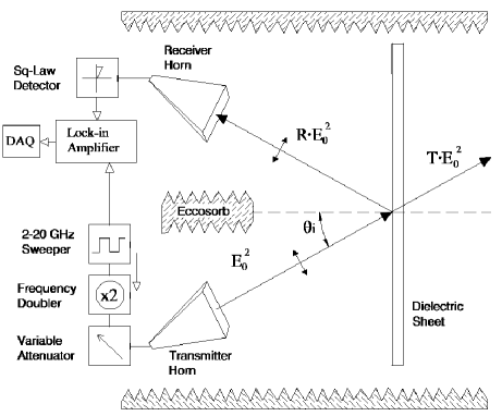
The experiments were performed in a small homemade anechoic chamber (see Figure 5.2), made of commercially available Eccosorb^® CV-3 [121]. Eccosorb CV-3 has a quoted reflectivity of less than -50 dB at frequencies up to 25 GHz, and a reflectivity of -34 dB at 107 GHz [122], which was adequate for our purposes. We fixed the incidence angle at $45^{\circ}$, which was the primary angle of interest to us. A standard-gain (25 dB) pyramidal feedhorn transmitted a signal of known frequency to a dielectric sheet approximately $20"\times 20"$ in area. The signal was generated by a commercial 2–20 GHz microwave sweeper coupled to a frequency doubler to obtain the $K_{a}$-band frequencies of 26-36 GHz. An identical horn was placed symmetrically about the sheet’s normal in order to receive the reflected waves. Reflected radiation from the room was found to be minimal. A thin piece of Eccosorb was placed between the two horns to minimize direct coupling between them. The transmitting source was swept through the $K_{a}$-band over a period of $100$ seconds, and the amplitude square-wave chopped at 1 kHz (this frequency was well above the 1/f knee of the system). The received signal was then sent to a lock-in amplifier and recorded by a computer using a simple data acquisition system. The reflected signal was quite small, and the lock-in technique enabled us to significantly reduce our sensitivity to 1/f noise in the system. A baseline reading was obtained using an aluminum flat instead of the dielectric sheet; the flat had near-perfect reflectivity and provided our normalization.

It was important to control systematic effects well; in particular, the imperfect absorption of microwaves by the Eccosorb walls of the anechoic chamber. By varying the Eccosorb configuration, we were able to virtually eliminate all spurious signals related to imperfect Eccosorb absorption. In the optimal configuration, tests with no reflector showed our system was capable of measuring reflection coefficients as low as a few $\times 10^{-5}$. The primary systematic effect was standing waves in the system, propagating between the source and reflecting surface. These were controlled (but not eliminated) by placing an attenuator between the sweeper and the transmitting horn.

Figure 5.3: Comparison between laboratory reflectivity measurements and theory on polypropylene. The displayed $1\sigma$ errors in the data are mostly systematic, arising from standing waves in the system. The uncertainty in theory is due to both thickness variations and uncertainties in the index of refraction. $R_{TE}$ corresponds to the upper set of curves (dashed), and $R_{TM}$ to the lower set of curves (dotted). Measurements were averaged into 1 GHz bins for convenience. (a) Results for 0.020” (0.51 mm) thick polypropylene; (b) Results for 0.003” (0.076 mm) thick polypropylene.

Figs. 5.3(a) and (b) show the results for the 0.020” and 0.003” sheets, respectively. The errors bars shown on the measured points are primarily due to standing waves in the system. The theoretical error contours drawn represent the thickness variations in our plastic sheets. We found that both of these commercial sheets had thickness variations on the order of 5%; because the reflection signal is roughly proportional to $d^{2}$, the resulting uncertainty in the calibration is $\sim$ 10%. Uncertainty in the index of refraction of the dielectric is even more important. Luckily, for our chosen material of polypropylene in the $K_{a}$ frequency band, the refractive index is known to an accuracy of at worst $\sim 2\cdot 10^{-3}$ [123, 124], which contributes negligibly to our errors. As Figure 5.3 shows, the measured curves match the theory quite well for the displayed polypropylene data. Teflon (not shown) worked equally well, having an $R_{TE}-R_{TM}$ of approximately $0.10$ for the $K_{a}$-band frequencies we tested.

In this section we sought to verify Equation (5.20) with laboratory experiments. The reader should note that we did not include any off-axis beam effects when calculating the theoretical predictions for these experiments. The general calculation would involve integrating over the antenna pattern of the transmitting and receiving horns, for each polarization state. Off-axis rays, reflecting from the dielectric at slightly different angles from the on-axis rays, will then slightly affect the measured reflection coefficients, due to the variation of the reflection coefficients of the dielectric as a function of angle. However, the remarkable agreement between the predicted (on-axis) and measured reflection coefficients indicates that this was a small effect.

5.4.2 The Emission Term

Oblique emission from a dielectric will in general be polarized (for a review, see for example [125]). For this calibration technique to work, either the emission must be known accurately (in both polarizations), or it must be negligible. The emission of a material is determined by both its thickness and loss tangent (or alternatively, its extinction coefficient), will vary as a function of viewing angle, and will generally be polarized (that is, $\epsilon_{TE}\neq\epsilon_{TM}$).

As discussed in §5.4, the complete way to determine emission involves calculating both $R$ and $T$ using the complex refractive index, and then using Equation (5.18) to find the absorption (which equals the emission in thermodynamic equilibrium); then the calibration signal can be calculated using Equation (5.16). For this approach to work, the complex index of refraction (and hence the loss tangent) must be known to reasonably good accuracy, and the surface must be smooth; if the surface roughness is too high, the emission polarization will be less than theory predicts [126]. Typically, the loss tangent is known only poorly. Luckily, the total emission can often be made small compared to the reflection/transmission terms by appropriate choice of dielectric material and thickness for the frequencies of interest; then one can simply ignore the emission terms in Equation (5.16).

An approximation for the total emission is [120]

$$\epsilon\ \approx\ \frac{2\pi n\tan{\delta}}{\lambda}\cdot\ d$$ (5.24)

where $d$ denotes the thickness of the emitter, and $\epsilon$ denotes the fraction of its thermodynamic temperature that is emitted; hence, it produces a brightness temperature of $T_{\epsilon}=\epsilon\cdot T_{S}$. As an example, the polar calibration used a 0.003” thick polypropylene sheet which had a loss tangent of $\sim 5\times 10^{-4}$, leading to $\sim$ 12 mK of total emission; this turned out to be small in comparison with the calibration signal and hence was neglected.

Figure 5.4: Ratio of the polarized radiation, $T_{pol}$, due entirely to reflection, to the brightness temperature in emission, $T_{e}$, of the dielectric sheet, for various materials, vs. $\frac{d}{\lambda}$, the ratio of sheet thickness to free-space wavelength. The six curves are for different materials and/or frequency ranges; dashed: teflon ($30-300$ GHz), dotted: TPX (30–270 GHz), solid-thin: polypropylene ($20-40$ GHz), solid-medium: polypropylene (40–270 GHz), solid-thick: polypropylene (270–900 GHz), dot-dashed: mylar (120–1000 GHz). The darkened box shows polar’s region in this parameter space. Loss tangents were adopted from [120].

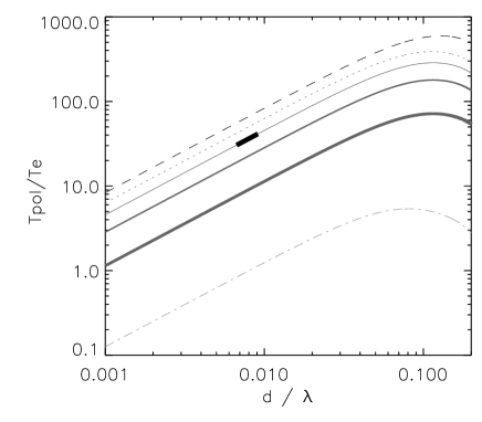
Figure 5.4 shows the ratio of the polarized reflection signal, $T_{pol}$, to the emission signal, $T_{e}$, as a function of $\frac{d}{\lambda}$. The higher this ratio is, the more safely emission can be neglected in calculating the calibration Stokes parameters. Notice that at higher frequencies and material thicknesses, emission matters less than at lower frequencies and thicknesses. This means that the smaller the desired polarization signal, the more emission will matter. This result may seem counter-intuitive, but it is directly evident from the reflection and emission equations; emission goes like $\frac{d}{\lambda}$, while typically the reflection portion of the signal goes like $\left[\frac{d}{\lambda}\right]^{2}$. In terms of absolute emission, polypropylene, polyethylene, TPX, and teflon are all useful. However, mylar’s high loss makes it non-ideal for this technique, unless one has good data on the directional emissivity of the material at the frequencies of interest.

5.4.3 Pitfalls

We discovered several pitfalls during the development of this calibration that should be avoided if possible. The first is to make sure the dielectric sheet is kept as taut and flat as possible. In our first version of the calibrator, we didn’t pay much attention to this and the plastic sheet had a slight bow in it. Laboratory results found this bowing to have a significant impact on the resulting calibration signal, causing it to deviate from theory by as much as $20\%$ for a barely-visible bowing. Reducing the bowing by increasing the tension in the sheet resulted in the signal matching theoretical predictions.

A second source of error was variation in material thickness. We found that, in practice, some of the materials we tested varied by as much as $10\%$ in thickness across a sheet; this is rather large and leads to a high uncertainty in the calibration signal, due to its approximate $d^{2}$–dependence. Sheets with manufacturing processes that lead to a more uniform thickness should be used if possible.

5.5 Daily Calibration Observations

Figure 5.5: The polar Dielectric Sheet Calibrator (DSC). The DSC could be rotated manually about the horn, and locked into any of 16 evenly-spaced positions.

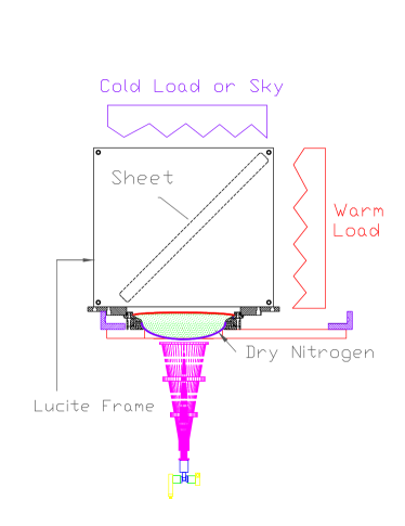
Now that we understand the theoretical and experimental basis of the calibration technique, let us discuss how it worked in practice. Calibrations were performed roughly once/day during periods of good observing weather. The dielectric sheet calibrator (DSC, see Figure 5.5) we built for observations had a lucite frame, and had several dielectric sheets that we could easily switch in and out: 3-mil polypropylene, 20-mil polypropylene, and a wire grid made of 8-mil wide copper strips deposited on 2-mil mylar. The DSC sat snugly on top of the vacuum window, and was rotated among eight different positions (one position every 45^∘); ideally, the polarimetric response would then be ($0$, $V_{max}$, $0$, $-V_{max}$, $0$, $V_{max}$, $0$, $-V_{max}$) for each of the eight positions, as the response varies as $\sin{2\theta}$. The resulting calibration coefficient is then given by:

$$\frac{1}{k_{i}}=\frac{(T_{H}-T_{C})(R_{TE}-R_{TM})}{V_{max}}\ \ \ \ \ \ [\frac{K}{V}]\ ,$$ (5.25)

since for these for frequencies in polypropylene, emission can be neglected in Equation (5.16c).

A full calibration consisted of techniques to calibrate all signal channels (including the total powers) and used these measurements to extract the calibration coefficients, system temperatures and NETs for each channel, as well as the overall $K_{a}$-band sky temperature. In order to accomplish this, the following procedure was repeated daily (in good weather). We placed each of the following ”loads” in front of the radiometer for the duration indicated:

• Pure Sky Load (1 min)

• Pure 77 K Eccosorb Load (1 min)

• Pure Ambient Eccosorb Load (1 min)

• DSC with sky, 300K loads (2 rev, 10sec/position)

• DSC with sky, 300K loads (2 rev, 10sec/position)

• Pure Ambient Eccosorb Load (1 min)

• Pure 77 K Eccosorb Load (1 min)

• Pure Sky Load (1 min)

The total-power channels were calibrated with a simple y-factor between 77 K and 300 K Eccosorb loads. Sky temperature was then extracted via the total power (now calibrated) sky measurements. System temperatures were determined from noise y-factor measurements (discussed in §5.2.4), and NETs were determined from the PSD of each channel viewing pure sky (applying the appropriate calibration). The entire calibration procedure took about fifteen minutes.

5.5.1 A Sample Calibration

Figure 5.6: A sample calibration signal, showing the response of the three correlator channels to the spinning dielectric sheet viewing a 300 K load to the side and a 10 K (sky) load above. The raw calibration signal is a function of frequency, leading to the different responses of the three channels. The angular labels correspond to the eight evenly-spaced positions of the DSC referred to in the text.

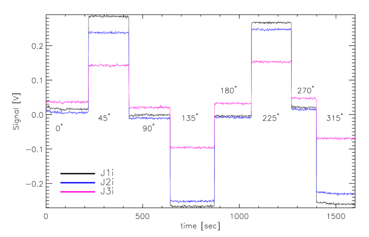
A sample calibration of the DSC viewing (sky ,300 K) is shown in Figure 5.6. You can see the signal-to-noise ratio is quite high; indeed, it is $\sim$ 100 for J1. Remember, these calibration signals are of order 500 mK! Note also that the strength of the calibration signal varies as a function of frequency, roughly according to Equation (5.23), as $f^{2}$. Our center frequencies of (27.5, 30.5, 34.0) GHz correspond to a calibration ratio of 1.0:1.23:1.53, for $J3$:$J2$:$J1$.

The Calibrator Background

Of course, a problem is immediately evident in the calibration plot. Besides slight overall offsets, which are expected as explained in §3.2.5, the signals are not quite the same when rotate 180^∘ in angle, nor are the signals all equal at multiples of 90^∘, which should correspond to no polarization. Although the exact source of this effect is unknown, we believe it to be related to beam-spillover to the calibrator frame, which was made entire of lucite. It is possible that via both reflection and emission, sidelobe pick-up contributed additional polarized signals to the radiometer during calibration; if these were not constant as a function of angle (say, due to the presence of the person calibrating), this could lead to the observed asymmetry, and have a non-negligible effect.

Thus, we believe there was a “background” associated with the calibrator that only manifested itself when the polarization signal generated by the dielectric sheet was $\lesssim$ 100 $mK$, as in the case of the 0.003” sheet we used for most of the season. Calibrations done at the beginning of the season with a 0.020” sheet, which itself produces close to 50 times as much signal, do not exhibit this effect. Therefore, we presume the effect to be only important in the case of the 0.003” sheet calibration.

Presumably, there is some small spurious polarization generated by the lucite calibrator frame, scattering radiation that is some mixture of sky and 300 K, and this mixture is dependent upon the orientation of the calibrator. In order to correct for the effect, calibrations done with the two sheet thicknesses were compared, and correction factors were derived for each channel. The correction factor was $\lesssim 2\%$ for J1 and J2, but was about $1.25$ for J3, such that the derived NET was lower than without performing the correction.

The errors on these corrections factors are based simply on the statistical variation in the correction factors between the $\sim$ 3 calibrations where correction factors could be derived. Unfortunately, this effect was not realized until well after the experiment had been dismantled , so we could not fully characterize it; the lesson is to always check your background, even if you think it is non-existent!

5.6 Atmospheric Correction

There is one final consideration in our calibration to be discussed. In addition to the correction factor for converting from brightness to thermodynamic temperature, there is also a correction factor due to atmospheric absorption. The actual antenna temperature we see on the ground is given by:

$$T_{ant}=T_{ant}^{cmb}e^{-\tau}\ +\ T_{phys}^{atm}(1-e^{-\tau})$$ (5.26)

where $\tau$ is the optical depth of the atmosphere, and is a function of both frequency and atmospheric conditions. $T_{ant}^{cmb}$ is the CMB antenna temperature, and $T_{phys}^{atm}$ is the effective physical temperature of the atmosphere. The atmospheric condition that most strongly affects $\tau$ in the $K_{a}$ frequency band is the precipitable water vapor content.

When we calibrate on the ground, the calibration signal is obviously not travelling through the atmosphere, and so receives no attenuation, but any astrophysical signal we receive will be attenuated by the factor $e^{-\tau}$. Hence, we must multiply all our calibration coefficients by $1/e^{-\tau}\simeq 1+\tau$, as $\tau$ will typically be small, less than 0.1 in our band.

The main question is then how to determine the optical depth at any observation time, for each of our three channels. If we had simply one large band spanning 26-36 GHz, we could use our total power channels as atmospheric monitors; then the optical depth is obtained via solving Equation (5.26). The physical temperature of the atmosphere, $T_{phys}^{atm}$, is typically $\sim$ 250 K, and varies very little. Thus, this method works over a whole band, but is not very helpful in determining the individual sub-band corrections.

Figure 5.7: Atmospheric emission profiles for different lineshape types, assuming 3 mm precipitable water vapor. The emission, $1-e^{-\tau}$, depends strongly on the lineshape assumption. This graph contains several prominent features: the atmospheric “windows” centered about 30, 100, and 150 GHz; the water lines at 22 and 182 GHz, and the oxygen lines at 60 and 119 GHz.

At this point, we utilize the atmospheric model by Erich Grossman, as implemented in his commercial $AT^{\copyright}$ software [127]. We fix the latitude and altitude to be those of our observing site, and vary the precipitable water vapor (PWV) content. However, the least well-constrained aspect of the model is the lineshape profile of the various lines contributing to the atmospheric absorption profile. This is illustrated in Figure 5.7, which shows the atmospheric brightness temperature from 0-300 GHz. There are four line profile shapes typically used: Full Lorentzian, VanVleck-Weisskopf, Zhevakin-Naumov (ZN) Harmonic Oscillator, and Zhevakin-Naumov Typo. The last of these was actually derived from a typographic error in the original paper on the ZN-Harmonic Oscillator lineshape, but was found to give reasonable, if somewhat pessimistic (large optical depth) values. All four profiles give similar results near the line peak; it is how they treat the “wings” of the line that is different. The Full Lorentzian and ZN-Harmonic Oscillator give virtually identical atmospheric profiles. In this work, we assume a ZN-Harmonic Oscillator lineshape profile, as it is a fairly ”middle-of-the-road” case, is recommended by the AT model author, and yields atmospheric antenna temperatures similar to those we measured in our total power channels.

Figure 5.8: Atmospheric emission with varying PWV. The PWV values are 0, 3, 9, and 15 mm, corresponding to the solid, dotted, dashed, and dot-dashed curves, respectively. Notice the rapid increase of the 22 GHz “water line” with increasing PWV. The vertical dashed lines correspond to our sub-band boundaries, labelled as shown.

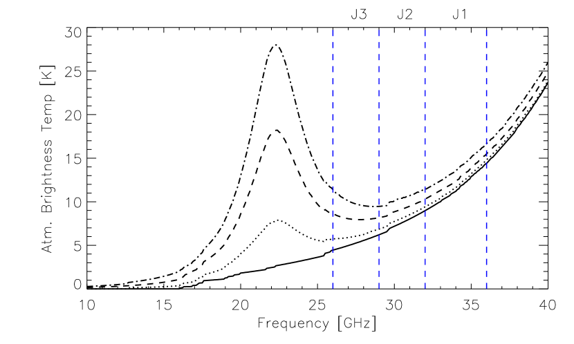
Figure 5.8 shows the effect of varying PWV across the $K_{a}$ band, given our lineshape assumption. We chose a sea-level temperature of 280 K, although changing this by $\pm\ 10K$ has only a small effect on the results. The 22-GHz “water line” is very striking as the PWV is increased. The large emission at higher frequencies is due to the 60 GHz oxygen line. By using this model, we can derive the atmospheric correction factor $e^{\tau}$ simply by knowing the water vapor content of the atmosphere. Figure 5.9 plots the emission, $1-e^{-\tau}$, for each of the $K_{a}$ sub-bands, where flat sub-bands are assumed for each channel. Note that the emission and hence the correction factor is highest in the J1 sub-band.

Figure 5.9: Atmospheric emission in the polar sub-bands, as a function of atmospheric water vapor.

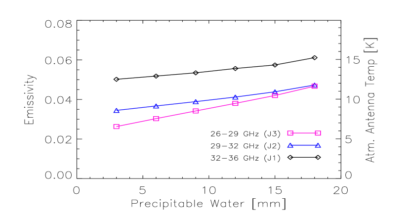
We combined the above model with water vapor measurements made by the Geostationary Operational Environmental Satellite (GOES) [128], which was publicly available for download hourly, in order to derive hourly atmospheric correction factors for each channel. The mean correction factors are given in Table 5.1, for good data only; that is, data that survived the quality cuts given in Chapter 7.

Channel	$\mathbf{e^{\tau}}$
J1	$1.0555\ \pm\ 0.0020$
J2	$1.0391\ \pm\ 0.0025$
J3	$1.0389\ \pm\ 0.0019$

Table 5.1: Atmospheric calibration correction factors, $e^{\tau}$, for each of polar’s three sub-bands, during periods of data that survive all quality cuts. For each channel, this results in a distribution of correction factors; the numbers listed are the mean plus or minus the standard deviation of those distributions. Because of the relatively small variation with precipitable water vapor content, a single correction factor was applied to each channel for the entire season.

5.7 Putting It All Together

Now that we have all the pieces of the calibration, let us put them together, so that not only will we understand where the full calibration comes from, but we’ll also get a better idea of the calibration uncertainty. The full calibration coefficient for each channel is given by

$$k_{i}=\frac{(T_{H}-T_{C})(\Delta R)}{\Delta V}\ \eta_{bright}\ \eta_{atm}\ \eta_{beam}$$ (5.27)

where the quantities in the equation are as follows:

• $T_{H}$: Hot Eccosorb load temperature

• $T_{C}$: Sky brightness temperature, sum of atmospheric + CMB temperatures

• $\Delta R$: $R_{TE}-R_{TM}$ for the channel, given by Equation (5.20)

• $\Delta V$: The voltage amplitude the channel passes through as the calibrator spins through 360^∘

• $\eta_{bright}$: The conversion factor from brightness temperature to thermodynamic temperature

• $\eta_{atm}$: The correction factor due to atmospheric attenuation of celestial signals

• $\eta_{beam}$: The correction factor due to beam spillover off the hot and cold loads during calibration

It is possible to place uncertainties on each of these terms in order to arrive at a final calibration uncertainty for each channel, although for certain terms the uncertainties are not particularly well known (e.g. , the beam spill-over correction). Estimates of all the above terms and their uncertainties have been compiled into Table 5.2, as well as the calculated final uncertainties in each channel’s calibration. Notice that the only uncertainties that really matter in the final calibration error budget are due to $R_{TE}-R_{TM}$ and the beam spill-over effect described in §5.5.1. The J1 and J2 final uncertainties are both roughly 10%, while the J3 uncertainty is significantly higher due to the beam spill-over effect.

Term	J1		J2		J3
$T_{H}\ -\ T_{C}$ 1		$\pm\ 4K$ (1.5%)		$\pm\ 4K$ (1.5%)		$\pm\ 4K$ (1.5%)
$\Delta R$ 2	$0.0024$	$\pm\ 8\%$	$0.0020$	$\pm\ 8\%$	$0.0017$	$\pm\ 9\%$
$\Delta V$ 3		$\pm\ \sim 1\%$		$\pm\ \sim 1\%$		$\pm\ \sim 1\%$
$\eta_{bright}$	1.0303		1.0243		1.0197
$\eta{atm}$ 4	$1.056$	$\pm\ 0.5\%$	$1.039$	$\pm\ 0.5\%$	$1.039$	$\pm\ 0.5\%$
$\eta{beam}$ 5	$0.98$	$\pm\ 2\%$	$0.99$	$\ \ {}^{+1\%}_{-2\%}$	$0.80$	$\ \ {}^{+5\%}_{-15\%}$
Final Uncertainty	$\pm\ 8.5\%$		$\pm\ 8.5\%$		$\ +11\%,\,-18\%$

Table 5.2: Values and uncertainties in all calibration terms from Equation (5.27), as a function of channel. For those terms that changed throughout the season, only the uncertainties are shown. Standard statistical error propagation was used to arrive at the final uncertainties.

• Uncertainty due to rough TP measurement of sky temperature, as well as interpolating to the given channel.

• Uncertainty due primarily to index of refraction and thickness of the dielectric.

• Uncertainty due to noise in channel, and offset drifts during each calibration.

• Larger error adopted because of uncertainty associated with lineshape profile.

• Uncertainty due to lack of knowledge of beam spillover location, and in measurement from 20-mil dielectric to determine correction factor.

5.7.1 Calibration Variations Throughout the Season

Figure 5.10: The calibration constants of our three signal channels (J1i, J2i, J3i) measured throughout the observing season, using the DSC with $T_{C}=sky$ and $T_{H}=300K$. The term cc denotes “calibration coefficient”. Some innate scatter, due to both system variations and human error, is evident in the plots. The J3 beam-correction factor has not been applied here.

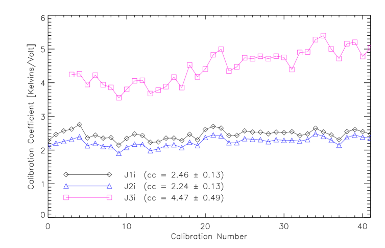
Figure 5.10 shows our $\sim$ 40 calibration measurements taken throughout the season. Overall, we were quite pleased with the stability. In the two best channels, J1i and J2i, the 1-$\sigma$ variation is about 5% over the course of the season. Computing a $\chi^{2}$ is uninformative, because the inherent uncertainty in each calibration is mostly systematic. There is some random error due to human error, such as not stopping the calibrator at the correct point. Also, as certain system parameters varied over the course of the season, such as the HEMT temperature, we do not expect these curves to be precisely constant. J3i’s calibration varied somewhat more, by about 10%, but this is still not enough to worry about it for the very same reasons.

For a section of data taken between two calibrations, we used the mean calibration coefficients of those two measurements. We opted this over a more complicated linear extraction because of its simplicity, and the fact that calibrations did not vary much between two adjacent calibrations.

5.8 Derivation of Calibration Signal Stokes parameters

Our goal in this appendix is to determine the Stokes parameters due to the electric fields generated by the dielectric sheet calibrator (DSC) as shown in Figure 5.1. Specifically, we would like to know $I_{x}$, $I_{y}$, $Q$, $U$, and $V$, where $I_{x}$ ($I_{y}$) is the intensity of the electric field polarized along the $\hat{x}$ ($\hat{y}$) axis. The Stokes parameter I is then simply given by $I=I_{x}+I_{y}$.

By looking at Figure 5.1, we see that the $\hat{x}$-axis corresponds with TE-polarized electric fields, of which there are essentially three: the TE-field from $T_{C}$ transmitted through the sheet, the TE-field from $T_{H}$ reflected from the sheet, and the TE-field emitted from the sheet itself. Similarly, the $\hat{y}$-axis corresponds with TM-polarized fields. Thus, we have

$$I_{x}=|t_{TE}|^{2}T_{C}+|r_{TE}|^{2}T_{H}+\epsilon_{TE}T_{S}\ ,$$ (5.28)

where $r_{i}$ is the ratio of the reflected to incident electric field polarized along $\hat{i}$ due to the sheet, and likewise $t_{i}$ is the ratio of transmitted to incident electric field polarized along $\hat{i}$. Using the fact that $|r_{i}|^{2}=R_{i}$ and $|t_{i}|^{2}=1-R_{i}-\epsilon_{i}$ (the latter being due to Equation (5.18)), we can recast Equation (A1) as

$$I_{x}=T_{C}+(T_{H}-T_{C})R_{TE}+(T_{S}-T_{C})\epsilon_{TE}\ ,$$ (5.29)

which is the form given in Equation (5.16). The derivation for $I_{y}$ follows the same format and yields

$$I_{y}=T_{C}+(T_{H}-T_{C})R_{TM}+(T_{S}-T_{C})\epsilon_{TM}\ .$$ (5.30)

Now we can use the fact that $Q=I_{x}-I_{y}$, which immediately leads to Equation (5.16c). Next, due to the rotation properties of Q and U we can write U as

$$U=I_{x_{45}}-I_{y_{45}}$$ (5.31)

where ${\hat{x}}_{45}$ refers the the axis rotated +45^∘ from $\hat{x}$, and ${\hat{y}}_{45}$ is the orthogonal axis. However, as the $\hat{x}$ and $\hat{y}$ axes are exactly aligned with the TE and TM states, the 45^∘-rotated axes will contain equal amounts of TE and TM fields, and their intensity difference will be zero. Thus we have

$$U=0\ .$$ (5.32)

Finally, we must consider the possibility of the sheet contributing a circular polarization signal V to our hypothetical polarimeter. We only expect this if there is some coherent phase delay between TE and TM polarizations, to give the final polarization state some ellipticity. This cannot happen from the unpolarized loads, but the emission from the sheet as seen at oblique angles will in general be elliptically polarized due to its imperfect transparency [125]; however, this will be proportional to the emissivity of the sheet and hence will be small enough in comparison to the other Stokes parameters that it can be ignored for the purposes of this paper, and we take

$$V\approx 0\ .$$ (5.33)

5.9 Derivation of Simplified $R_{TE}-R_{TM}$

The purpose of this appendix is to derive the quantity $R_{TE}-R_{TM}$ under the simplifying assumptions that $\lambda\gg t$ (which is equivalent to $\delta\ll 1$), and $\theta=45^{\circ}$. Applying the latter assumption to Equations (5.21) and (5.22) yields

$$\gamma_{TE}^{2} = n^{2}-0.5,$$ (5.34a)

$$\gamma_{TM}^{2} = \frac{1}{n^{4}}\left(n^{2}-0.5\right)$$ (5.34b)

and

$$\delta=kt\sqrt{n^{2}-0.5}\ .$$ (5.35)

Substituting these expressions into Equation (5.20), and requiring that $\delta\ll 1$, we have

$$R_{TE} \simeq (kt)^{2}\frac{(n^{2}-1)^{2}}{2}$$ (5.36)

$$R_{TM} \simeq (kt)^{2}\frac{(n^{2}-1)^{4}}{8n^{4}}$$ (5.37)

Finally, solving for $R_{TE}-R_{TM}$ we find

$$R_{TE}-R_{TM}\simeq(kt)^{2}\frac{(n^{2}-1)^{2}}{8n^{4}}\left[4n^{4}-(n^{2}-1)^{2}\right]$$ (5.38)

which factors into

$$R_{TE}-R_{TM}\ \simeq\ \left(\frac{\pi ft}{c}\right)^{2}\frac{(n^{4}-1)(n^{2}-1)(3n^{2}-1)}{2n^{4}}$$ (5.39)

as desired.

Chapter 6 Observations and Weather Data

polar was deployed into the field on March 1, 2000. After a period of setting up, calibrations, and systematics tests, observations were begun in earnest on March 11, and continued through May 29, 2000. polar was situated at the Pine Bluff Observatory, in Pine Bluff, Wisconsin (latitude = 43.08^∘, longitude = 89.69^∘W). This is a small astronomical site that the UW-Madison Department of Astronomy owns and operates; it sits on a small hill in the country, circumscribed by trees that are all less than 10^∘ above the horizon. Our observing philosophy was to always take data unless it was raining or snowing. This was possible through the internet-based dome operation system described in §4.4.1; this system allowed for fast response times, sometimes enabling us to take data very close in time to severe weather .

6.1 Observing Region

polar utilized a simple zenith drift scan. The instrument was initially levelled with the jacks on each of the four corners of the mount, to within 0.2^∘ of the actual zenith.The zenith scan resulted in an observation region spanning right ascensions $0h$ to $24h$, at a declination equal to our latitude of 43.08^∘. For our beamwidth of $\sim$ 7^∘, this corresponds to approximately 38 uncorrelated pixels on the sky. The path of our observing strategy is shown in Figure 6.1. Note that it passes through both high– and low– galactic latitude regions. The low galactic regions are interesting as they are likely to house the strongest polarized foregrounds, especially the region around right ascension 20h, which corresponds to the very bright radio source Cygnus A, and is very obvious in Figure 6.1. In the actual CMB analysis, we eliminated all regions with galactic latitude $|b|<25^{\circ}$.

Figure 6.1: The polar scan strategy, overlaid on the 408 MHz Haslam Synchrotron map, plotted in galactic coordinates. The off-colored portion of the scan path denotes the area where galactic latitude $|b|>25^{\circ}$; we ended up cutting all data taken below this point to avoid galactic contamination.

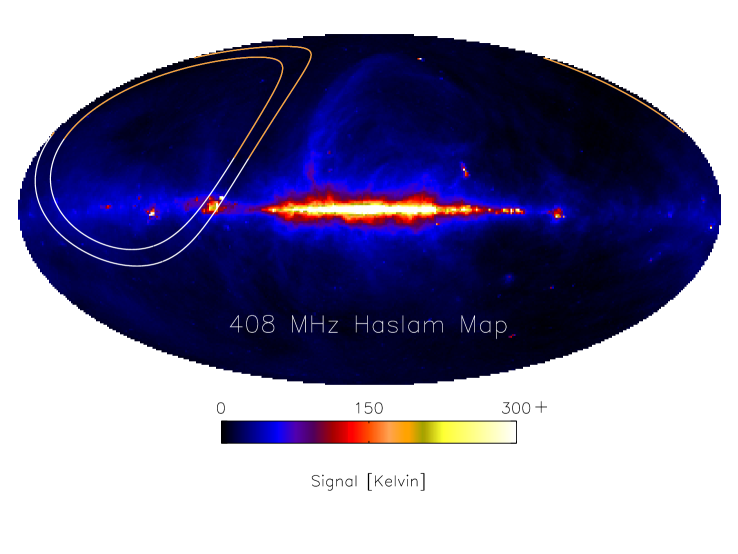
6.2 Structure of the Data

polar collected approximately 750 hours of data during the 2000 observing season. There were three principle operators of the instrument. Every day one of the operators would drive to the Pine Bluff site, check on polar, perform a calibration (described in §5.5), and of course, fix things when they broke.

Name	Description	Duration
Section	One deployment, between calibrations, during which the dome was open and data was recorded. There were 49 total sections in this data set.	2-48 hours
Hour File (HF)	One data file, containing 9000 samples/channel. The Header of the file contains data/time, pwv, and weather information.	7.5 min
Rotation	A single rotation’s worth of data, defined between consecutive AOE pulses. Typically contained 630 samples.	30.6 sec
Sample	A single sample of data, containing one recording of each of the sixteen data channels.	0.05 sec
Submap	Sky map (signal vs. RA) derived from the good data within one section.	2-15 hours

Table 6.1: The various levels of polar data organization.

The structure of the data is described in Table 6.1. Periods between calibrations during which we were acquiring data were called Sections. During acquisition, data were recorded to files 7.5 minutes in length, called Hour Files (hereafter HF). As we took data at 20 Hz, there were precisely 9000 samples per channel recorded in one Hour File. Additionally, several pieces of information were recorded in the header of each HF:

• Date and Time measured by a commercial time-stamping card.

• Precipitable Water Vapor, as extracted by the GOES satellite[128], for the region over Pine Bluff, WI.

• Latest weather information from the polar weather station: temperature, relative humidity, wind speed and direction.

When the instrument was spinning normally, it rotated between 13 and 14 times per HF. Throughout the course of the season, polar rotated more than 90,000 times.

6.3 Weather Conditions

Some members of our team had reservations about performing sensitive CMB observations from a site that traditionally sees fairly wet and unstable weather. Most ground-based CMB experiments are performed at high, dry sites, such as the Atacama desert in Chile, the South Pole, or the beautiful Tenerife island in the Mediterranean. However, as described in Chapter 2, the atmosphere is not expected to be polarized, and thus ground-based polarization observations are theoretically possible. Of course, increased sky loading will add to the noise of our experiment, requiring longer integration times to see a given signal.

Figure 6.2: Precipitable Water Vapor (PWV) and Cloud Cover for Pine Bluff, WI, as determined from hourly GOES satellite data. (a): Shows the PWV histogram for the years 1997, 1998, and 2000, separated into seasons. (b): Shows the same information as (a), but in integrated form (fraction of time less than a certain value). (c): Displays the cloud cover percentage histogram for 2000. As cloud cover was not very seasonally dependent, the full year is displayed as a single curve. (d): Same as (c), but in integrated form. All data were provided by Gail Bayler and Gary Wade at the UW-Madison Space Sciences and Engineering Center.

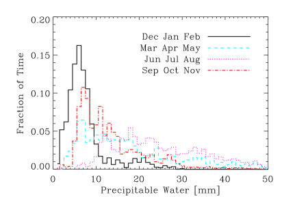
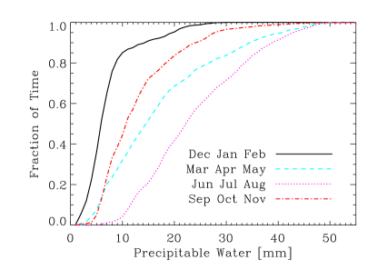
We compiled data on the Pine Bluff area from both the National Weather Service and the GOES satellite data served by the Space Sciences and Engineering Center at UW-Madison [128]. The GOES-8 data proved most useful as it was recorded hourly, and typically hit a patch with area 5 km by 5 km, within 20 km of Pine Bluff. It provided cloud cover fraction of the area, as well as precipitable water vapor (PWV) column height (along with a host of other weather variables). We acquired all the data for 1997, 1998, and 2000 on precipitable water, but only the year 2000 for cloud cover information. These data are displayed in Figure 6.2. Figures 6.2 and (c) show PWV and cloud cover fraction histograms, while Figures 6.2 and (d) show the same information in “integrated” form; that is, they display the fraction of time the variable was less than a certain value. PWV showed a strong seasonal dependence; in the figures, the three years of data are averaged, but separated by season as shown. Notice that in the winter, more than 50% of the time has PWV $<$ 5 mm, and almost 90% less than 10 mm. This is in stark contrast to summer, where around 95% of the time the PWV is greater than 10 mm! Clearly, summer is a bad time for CMB observations in Wisconsin. Spring and Autumn lie in between, but are still less than ideal. It is perhaps noteworthy that Autumn is markedly better than Spring in terms of PWV.

Cloud cover fraction is not seasonally dependent, but does exhibit a bimodal distribution, with more than 35% of the time showing totally clear weather. However, about 15% of the time is categorized as completely overcast (and will likely be useless for CMB observations). The “partially cloudy” days account for the other 50% of the distribution.

Figure 6.3: Precipitable Water Vapor during Observation Season. (a) shows the PWV histogram during the observing season, while (b) shows the same data in integrated form. More than 50% of this period has PWV less than 10 mm.

While the general Wisconsin weather displayed in Figure 6.2 is interesting in its own right, what were these values during actual observations in the Spring of 2000? The cloud cover distribution is virtually unchanged, and the water vapor follows the general Springtime trend, as shown in Figure 6.3. They are consistent with the previous distributions for Spring weather in Wisconsin. We leave it to the next chapter to discuss the effects of the weather upon the data, but the general conclusion here is that there will be a reasonable number of clear, dry days in Wisconsin, even in Autumn and Spring. Sensitive measurements of CMB polarization are clearly possible from the ground, even from a relatively poor site such as Wisconsin.

Chapter 7 Data Selection

The polar observing season contained a large diversity of weather conditions, and this led to a correspondingly large diversity of data quality. This is in stark contrast to a typical balloon or satellite mission, where often most of the data set is of the same quality, and various statistics of the data do not change much over the data set. For polar, we observed through cloudy, humid conditions as often as through clear, dry conditions.

Thus, developing robust data selection techniques was one of the most critical tasks in the data analysis pipeline. We used standard techniques of time series analysis to look at the data in different ways, in order to assess its quality and to develop criteria on which to cut. Unfortunately, because of the data’s diversity, we were not able to arrive at a single selection criterion; rather, we developed a battery of conditions that the data must pass before being accepted. Our underlying philosophy was to cut “more rather than less”, to ensure a final data set of the highest possible quality.

7.1 Data Analysis Overview

There are many measures of data quality, but the critical thing for this experiment is that polar rotated. It is then natural to describe the output of polar’s correlator channels in the following form:

$$y(t)\;=\;I_{0}+C\cos{\omega t}+S\sin{\omega t}+Q\cos{2\omega t}+U\sin{2\omega t}+n(t)\qquad$$ (7.1)

where $\omega=2\pi f=0.2055\;rad\;s^{-1}$ was polar’s (angular) rotation frequency. The constant offset $I_{0}$ is due to coupling of the unpolarized total power signal into the correlators via the nonzero cross-polarization of the OMT described in §3.2.5. This offset term was typically 10-100 mK, depending on the channel; during good weather its stability was better than 0.6 mK per hour.

$C$ and $S$ are signals modulated at the rotation frequency (referred to hereafter as $1\phi$ signals), and can be caused by various types of ground pickup and other systematic effects. During good weather, there is often no “offset” associated with $C$ or $S$. An offset is quite conceivable, as any type of ground-source picked up in the sidelobes of our beam would have a strong component at $1\phi$. We often saw quite strong signals at the $1\phi$ frequency, but these signals were not ever particularly stable, mainly being associated with time-varying atmospheric conditions.

The signal we want to extract from our raw data is the astrophysical polarization signal in terms of $Q$ and $U$, and this corresponds only to signals modulated at twice the rotation frequency (hereafter $2\phi$). Thinking in frequency space, only signals modulated at this particular frequency can produce true polarization signals, and all other frequencies will be rejected in the analysis. The next chapter will discuss how this extraction was done in practice.

Many effects can conspire to contaminate the $Q$ and $U$ signals, be they instrumental, atmospheric, or celestial. In general it was not possible for us to cut bad data based on a single quantity that would apply to all causes of bad data. In fact, it was often difficult to determine the precise cause of bad data. This last statement begs the question, what precisely is “bad data”? The simple answer is any data with a non-cosmological contribution to our signal, that mimics a cosmological signal in a way that we cannot account for and remove. For instance, attenuation by the atmosphere scatters CMB photons as described in §5.6; but the effect is calculable, and does not (in principle) add a spurious polarized component. On the other hand, observing a finite, asymmetric cloud will lead to a spurious signal if we have an asymmetric beam, which we do at some small level. This will lead to an apparent signal in $Q$ and $U$, and this signal will change as the cloud moves through the beam. This is too difficult to model for and subtract out; therefore, the data must be cut.

The rest of this chapter will describe the various criteria we established, to separate the “good” data from the “bad”. I use quotes here with a purpose; “good” is a relative term, and in some sense the argument is circular because we define what is good data with the cuts will we establish. Table 7.1 lists all of the cut criteria used in polar; the entries in the table will be described throughout the rest of this chapter.

Cut Type	Remaining	Additional Cut	Individual Cut
No Cuts (full data set)	746.5 (100%)	0 (0%)	0 (0%)
Sun Elevation $<\ 20^{\circ}$	458.6 (61.4%)	287.9 (38.6%)	287.9 (38.6%)
Moon Elevation $<\ 50^{\circ}$	430.8 (57.7%)	27.9 (3.7%)	60.6 (8.1%)
Dew Cut	348.4 (46.7%)	82.4 (11%)	105.4 (14.1%)
Proper Rotation	346.8 (46.5%)	1.6 (0.2%)	13.8 (1.8%)
$1\phi_{r}\ <\ 2.1$	238.1 (31.9%)	108.7 (14.6%)	387.7 (51.9%)
$\zeta\ <\ 4.0$	210.2 (28.2%)	27.9 (3.7%)	303.9 (40.7%)
1/f Knee $<.060$ Hz	204.8 (27.4%)	5.4 (0.7%)	294.9 (39.5%)
Spike Two $<\ 5\sigma$	195.8 (26.2%)	9 (1.2%)	122 (16.3%)
Galactic Lat $>\ 25^{\circ}$	152 (20.4%)	43.9 (5.9%)	398.6 (53.4%)
Nearest Neighbor Cut	113.3 (15.2%)	38.7 (5.2%)	N/A
8 consecutive HFs	94.8 (12.7%)	18.5 (2.5%)	N/A
Duration $\geq\ 3$ Hours	78.1 (10.5%)	16.7 (2.2%)	N/A
Remove Q,U Spikes	77.3 (10.4%)	0.8 (0.1%)	N/A
Executive cuts	71.1 (9.5%)	6.2 (0.8%)	N/A

Table 7.1: Effect of various data cuts. The data set was viewed as three independent data sets (one for each channel), and shown are the cuts for this entire data set as an average of the individual channel cuts. Remaining is the amount of data left after that cut and all the cuts above it have been applied; Additional Cut is the amount of data cut at that stage; Individual Cut is the amount of data that would have been cut if that particular criterion were the only one applied. Thus, many cuts are overlapping. Of the 750 hours of data taken, only about 10% survived our cut criteria.

7.2 Data Selection Techniques

7.2.1 The Fiducial Data Unit

Before deciding those statistics upon which to cut, one must ponder the question of the time scale over which to cut. That is, do we simply remove individual data points we do not like? Or variable-length segments of data? If we cut one channel, do we cut them all?

We chose to cut at the hour-file (HF) level of the data, and we did this for several reasons. The simple answer was convenience: that is how our data were packaged. Another reason was that an HF contained 9000 samples/channel, which is a large enough number to get a good representation of the low-frequency power spectrum of the data during that particular HF. This was important because our mapmaking technique (described in Chapter 8) needs to know the noise properties of the data in order to turn the data into a map. We could also have cut on individual rotations of the system, but the mapmaking technique didn’t work nearly as well on individual rotations, so we stuck with full hour files.

Finally, we chose to perform the analysis on each of our three sub-bands individually, and thus we ended up cutting somewhat different portions of the data for each channel. Our channels exhibited fairly different responses to spurious signals and systematic effects, in particular channel J3, which often showed contamination when J1 and J2 did not. In order to save many “good” sections of data in J1 and J2, many of our data-based cuts applied to each channel individually.

7.2.2 Weather-Based Cuts

The first level of cuts was weather-based. Remembering that our philosophy was to always take data if possible, it is not surprising that much of our data were taken during periods of highly non-ideal weather conditions: high water vapor or humidity, rapidly changing temperature, strong winds, and diverse types of cloud cover, as well as the sun or moon being close to our main beam. Most of these conditions have a mechanism to contaminate our data, and thus it is important to consider each of these mechanisms and understand at what level they contaminate the data, and then remove these periods when the contamination is unacceptable.

Dew on the Window

The first issue was dew formation on the optics, a common problem in ground-based experiments. Specifically, when the relative humidity reached 95% or so for a long period of time (an hour or more), moisture would condense on the top surface of the window (namely, the layer of Volara). This immediately led to a strong polarization effect in the data, as shown in Figure 7.1. Most likely ambient (300 K) radiation was scattered off the layer of water; differential scattering coefficients coupled with a beam or ground asymmetry would lead to a spurious polarization signal.

This problem didn’t manifest itself until later in the season, when conditions became warmer and wetter, and we never came up with a good moisture-prevention system for the window surface. However, most characteristics of our data got worse during periods of high humidity, and thus it is quite likely that even absent this spurious polarization, data through a wet atmosphere would not have been useable. Of the 750 hours of recorded data, dew contaminated approximately 105 hours, or about 14% of the data set. As it had such a striking and characteristic effect on the data, it was simply removed by hand.

Figure 7.1: The Effect of Dew on the time stream. All three in-phase correlator bands are shown. Not only does dew on the window increase loading, but it generates a strongly polarized signal, presumably by scattering 300 K radiation into the system, and partially polarizing it. It is interesting to note that the resultant polarized signal is largely independent of frequency.

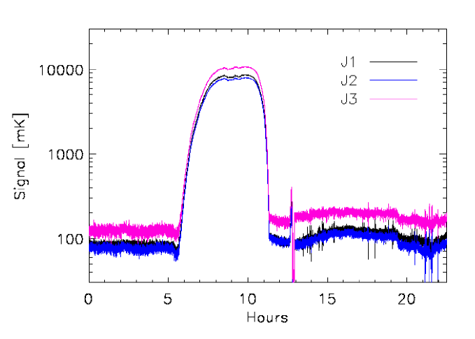
The Effect of Clouds

Clouds had a large effect on the correlator channels that was often visible directly in the time stream. Clouds are essentially non-uniformities in the three-dimensional water/ice field in the sky through which we observe. A patch in this field with a high but asymmetric water/ice content can induce a false signal, as our beam pattern is slightly asymmetric; thus, as we rotate, the asymmetric beam convolved with the asymmetric cloud will produce an offset that varies with rotation angle, and will in general have components at both $1\phi$ and $2\phi$. This suggest that data taken through thick clouds should be cut.

Unfortunately, we were unsuccessful in developing a good cloud monitor. Data containing some cloud cover information is available from both the National Weather Service (NWS) and the GOES-8 satellite. We found that neither correlated particularly well with periods of bad data. The NWS data were taken from the Dane County airport, roughly 35 km from our site. The GOES data were in the form of fields 5 km x 5 km wide, but typically the closest such field was about 20 km from our site. As cloud cover varies substantially over these distances, our cloud cover data are of little use as a cut statistic. As our only alternative, we opted to cut directly on statistics of the data themselves. These statistics are described in §7.3.

Sun Spikes

Figure 7.2(a) shows an 18-hour segment of time-ordered data, with the sun elevation overplotted. It is evident that the noise characteristics of the data are radically different when the sun is more than 30^∘ above the horizon. Plotting the power spectrum of two segments of the data (Figure 7.2(b)), when the sun is high and low, confirms this, and shows the noise properties get much worse at all frequencies, and significant $2\phi$ noise is added, which is unacceptable.

(a) Solar Contamination in the Time Stream

(b) Solar Contamination in the Power Spectrum

Figure 7.2: The Effect of Solar Radiation on the Data. (a) shows the effect on the time stream. When the sun climbs higher than about 20^∘ in the sky, some sun-related effect comes into play, increasing the noise and generating a spurious polarization signal. This is evident in (b), which displays the power spectra of a two segments of data, when the sun elevation is low and high.

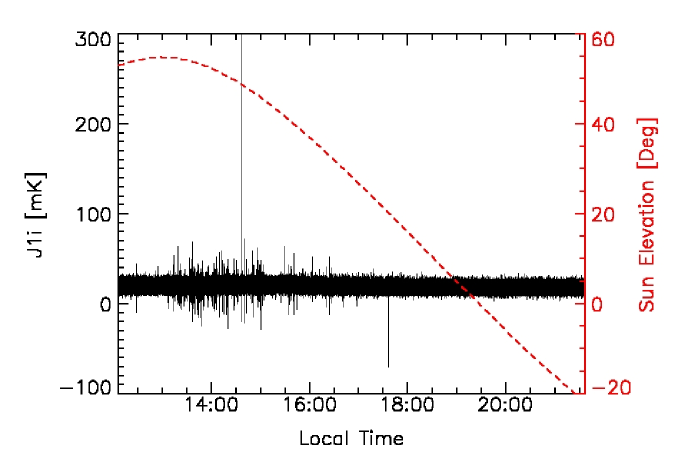
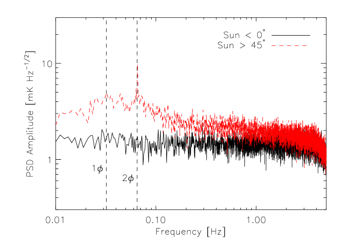
Based on the geometry of the cone, some solar radiation will enter when the sunlight can just make it over the outer (fixed) groundscreen and strike the inner ground screen. This happens at an elevation of $\sim$10^∘. However, this is a very tiny effect, because for this light to make it into the horn, it must scatter many times off the inner ground screen as it “runs around” the perimeter of the screen; it will then be mostly absorbed. Below this elevation of 10^∘, solar radiation must undergo a double diffraction to enter the system. The amount of sunlight reaching the horn then steeply increases as the sun climbs higher into the sky, until the sun’s elevation reaches $\sim$40^∘, at which time radiation from the sun can directly enter the horn. We found that, in practice, sun contamination was undetectable below a solar elevation of 30^∘. To be conservative, we eliminated all data taken with the sun more than 20^∘ above the horizon. As we attempted to take data 24 hours per day, this represents a sizeable 38.6% of our data, or $\sim$ 288 hours.

Recent additional evidence shows that this sun-correlated effect may actually not have been an optical effect caused by the sun, but rather was related to an increase in temperature. It appears that some electronic effect was initiated when the system was too hot; this could have been related to our heating temperature pads, but it is unclear at this point. What is clear is that this effect occurred during the daytime and late afternoon, and thus all of these periods had to be eliminated from the analysis.

One unfortunate consequence of our scan strategy was that much of the data near the galaxy crossings had to be eliminated due to sun and dew contamination, in particular the bright region near Cygnus A. It is conceivable we could have seen this region in polarization with reasonable integration time on it, but sun and dew contamination ruled out this possibility.

Moon Cut

The moon is a bright microwave source, corresponding to an emission temperature of roughly 220 K. Its emission is dependent upon frequency, phase, and polarization. The standard model of lunar emission at microwave frequencies is Keihm’s 1983 model [129]. Using this model, the COBE team calculated the lunar emission in both polarization states at the three COBE DMR frequencies, and showed that the polarization temperature at 31 GHz of the moon (viewed as a point source) is $\lesssim 1K$ [130]. We have reproduced their model in Figure 7.3.

Figure 7.3: Model of Lunar Emission at the frequencies 31, 53, and 90 GHz. The solid and dotted curves show the two different emission polarizations. Notice that they differ by approximately 1 K on average, independent of frequency. Reproduced from the COBE-DMR team, reference [130].

Figure 7.4: Lunar Contamination. This model assumes the moon has a 1 K polarized emission temperature at 30 GHz, when viewed as a point source, and is based on the assumptions of Bennett et al., 1992 [130]. We further assume attenuation only by the feedhorn beam pattern for this range of lunar angles. The figure shows that it is desirable to have the moon more than 40^∘ from the main beam.

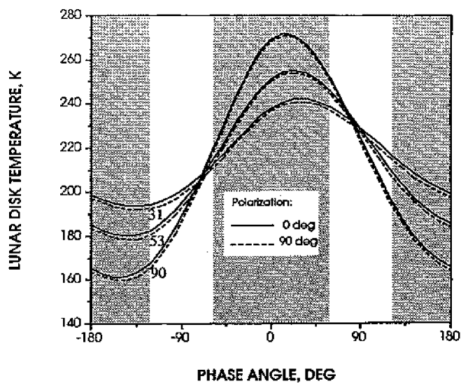
Let us now attempt to estimate how polar will view this emission. If we see the fully polarized effect, it will be attenuated by our beam function at the very least, and ground shields will only increase the attenuation. Modelling the moon as a point source in our beam (0.5^∘ is much less than 7^∘, so this is indeed a valid model), we can then estimate the polarization signal we will see as a function of moon elevation (or alternatively, angle from the boresight). Figure 7.4 shows this estimate, assuming an azimuthally-symmetric beam and a 1 K polarized lunar brightness temperature. When the moon is more than approximately 40^∘ from zenith, it cannot shine directly on the feed horn; a single diffraction over the rotating inner ground screen is required. Assuming this provides at least an extra 20 dB of shielding, we can safely assume lunar signals are negligible at elevations below 50^∘.

The moon’s highest elevation in Wisconsin is about 70^∘, and during our observation season the highest lunar elevation was 68.4^∘, corresponding to an angle from the zenith of 21.6^∘. We removed all data when the moon was more than 50^∘ in elevation; this corresponds to about 8% of the data. However, taking into account its overlap with other cuts, it only cuts about 3.7% of the total data set (28 hours).

Galaxy Cut

At low galactic latitudes, there is the possibility of a serious galactic foreground. We hoped to bypass this “demon” by cutting all data occurring below a certain galactic latitude. Thus, we elected to cut any data with galactic latitude $|b|<25^{\circ}$. This did not cut a significant amount of data in the end, but we felt it was important to have a well-defined section of sky where hopefully foreground contamination is kept to a minimum. Figure 6.1 from the previous chapter shows this cut overlaid with our scan strategy, on the 408 MHz Haslam synchrotron map. Clearly, this area of sky appears to be of much lower radio emission than the low galactic latitude regions.

7.2.3 System-Based Cuts

Although in principle most experiments have cuts based on equipment failure, high system temperatures and the like, we only had to perform two system based-cut because our systems generally operated as expected throughout the season. The first was cutting data whenever the clamshell dome was closed, although these data were cut right at the beginning of the analysis and was never included in what we called the “data set”. The second system-based cut was removing any HFs during which the system wasn’t rotating for the entire file, or the rotation was unnaturally slow or jittery. These primarily occurred at the beginnings of deployments, when we started taking data and then began system rotation. This cut accounts for about 1.8% of the data, and is referred to as “Proper Rotation” in Table 7.1.

7.3 Deeper Cuts

The above three sections deal with data problems that were quite simple to recognize and remove. According to Table 7.1, the sun and dew cuts have removed close to 50% of the data we took during 2000. However, many spurious signals remain lurking in the data. Sometimes they are associated with clouds, or high humidity, or other weather-related events, but sometimes they are not, and it is our job to identify and remove them.

7.3.1 The $1\phi$ Cut

The first powerful statistic that we learned correlated with spurious polarization signals was a high $1\phi$ signal (signals modulated at precisely our rotation frequency). Recall that only signals modulated at twice our rotation frequency can correspond to true polarization signals; thus, a signal that has harmonics at both $1\phi$ and $2\phi$ cannot correspond to a true celestial signal.

As an example, consider Figure 7.5. The left-hand (a) panel shows a classic, featureless white noise power spectrum, taken during a period of good weather for channel J2i. But as the weather gets bad, due to clouds, sun, or something else, features at the $1\phi$ and $2\phi$ frequencies appear, in addition to 1/f noise, as shown in Figure 7.5.

Figure 7.5: Low frequency power spectrum of two sections of data. Panel (a) shows a featureless, white noise power spectrum when the weather is good and systematic effects are low. Panel (b) displays a period when clouds appeared: in addition to 1/f noise increasing slightly, noise at the $1\phi$ and $2\phi$ frequencies appears as well. This motivated our using the height of the $1\phi$ peak as a cut statistic.

We computed the heights of each of the $1\phi$ peaks for every hour file in the data set (and for each channel). This was performed as follows: a given HF and data channel gives a 9000-element data set, for which we wish to calculate the low-frequency power spectrum. We use the standard, FFT-based periodogram construction of the power spectrum. With this algorithm, the highest frequency resolution given these parameters is $2/9000=2.22$ mHz. Recall that $f_{1\phi}=32.5$ mHz. However, a significantly better reconstruction of the power spectrum can be performed, at the expense of some degradation in frequency resolution, by splitting up the data into several overlapping equal-length segments, and averaging the power spectrum of each. A full discussion of these techniques is given in the classic Numerical Recipes [111], chapter 13.

Figure 7.6: $1\phi$ and $2\phi$ Fluctuations vs. Time, for channel J2i. The high degree of correlations between the two rotational harmonics is evident. The $1\phi$ statistic cannot correspond to a true sky signal, thus motivating its use as a cut statistic.

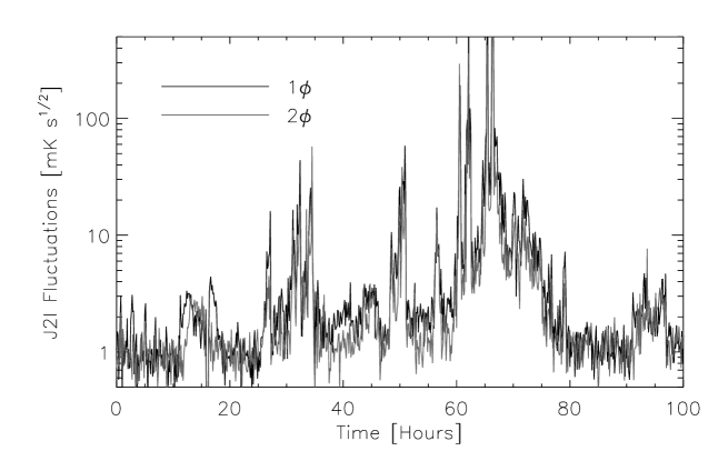
We found that, in practice, this technique gave very similar results to direct Fourier extraction of the $1\phi$ and $2\phi$ components. Figure 7.6 displays the $1\phi$ and $2\phi$ statistics through a 100–hour section of the observing season; periods of sun, moon, and dew have all been removed. The correlation coefficient between the $1\phi$ and $2\phi$ statistics are 0.73, 0.89, and 0.93 for channels J1i, J2i, and J3i, respectively. This strongly motivates a cut based on the $1\phi$ statistic. However, because we found the base noise level to fluctuate somewhat, we defined statistics relative to the base noise level, which will refer to as $1\phi_{r}$ and $2\phi_{r}$, where the ’r’ stands for ’relative’.

Figure 7.7: Histogram of $2\phi_{r}$ data for channel J2i. The solid (black) line represents all the data, with sun, moon, and dew-contaminated data removed. The dotted (red) line is the same data set for the QPC channel J2o; it can be thought of as the ideal $2\phi_{r}$ distribution for white noise. The dashed (blue) line is the $2\phi_{r}$ data after the $1\phi_{r}<2.1$ cut was applied. Notice that a large fraction of the tail of the distribution has been removed, but a small portion still remains.

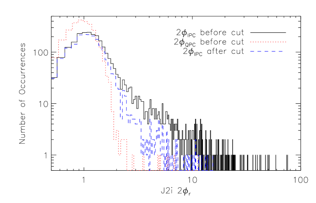
Figure 7.7 shows a histogram of the $1\phi$ and $2\phi$ data relative to the NET of each hour file (this is to remove the effects of gain drifts). A value of $1$ thus denotes a flat (white) spectrum; Monte-Carlos of Gaussian white noise show that this statistic should be $1.0\pm 0.27$. We cut whenever $1\phi_{r}>2.1$; this is more than $4\sigma$ from the mean for white noise.

Figure 7.8: $2\phi_{r}$ vs $1\phi_{r}$ for each the data channels J1i, J2i, and J3i. Periods contaminated by sun, moon, and dew have been removed. The vertical dashed line shows the $1\phi_{r}\ <\ 2.1$ cut level.

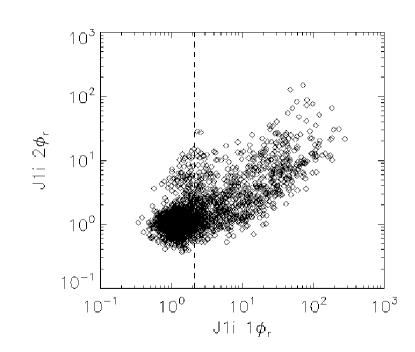
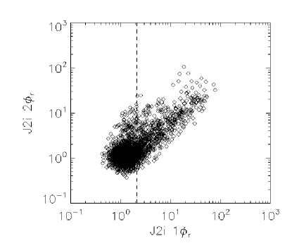
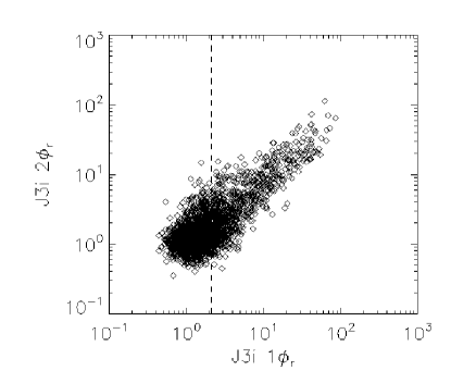
Figure 7.8 displays the same data, but plots $2\phi_{r}$ vs. $1\phi_{r}$; the cut level is shown as the dashed vertical line. Again, the high degree of correlation between the two quantities is obvious in all channels. Using $1\phi_{r}<2.1$, an additional 109 hours, or about 15% of the total data was cut.

7.3.2 Additional Selection Criteria

It is apparent from Figure 7.8 that there will still be some residual data points with high $2\phi_{r}$, regardless of the $1\phi_{r}$ cut. This motivated us to examine additional statistics that may also be correlated with the $2\phi$ level, and therefore may serve as useful data selection criteria. The next section will briefly describe each of these statistics.

The Zeta Cut

Auto-correlation is a powerful and illuminating technique for viewing data. The auto-correlation $C(y)$ of a data set $y$ is intimately connected to the power spectrum $S(\nu)$ via the Wiener-Khincin theorem [111]:

$$C(y)\Longleftrightarrow|S(\nu)|^{2}\ .$$ (7.2)

That is, the autocorrelation function $C(y)$ and power spectrum $|S(\nu)|^{2}$ of any data set form a Fourier transform pair, and hence the information in one is the same as the information in the other. A rise in 1/f noise leads directly to a higher “floor” in the autocorrelation. We used that fact to our advantage and defined the following statistic for each HF of data:

$$\zeta\ \equiv\ \frac{\sum_{lag=1}^{1000}{C(y_{in})}^{2}}{\sum_{lag=1}^{1000}{C(y_{quad})}^{2}}$$ (7.3)

where $y_{in}$ denotes data from an in-phase (IPC) channel and $y_{quad}$ denotes data from the corresponding quad-phase (QPC) channel. Equation (7.3) may seem a rather arbitrary definition, but it is fairly easy to analyze what it does. Using the Wiener-Khincin theorem, we can think of any timescale as corresponding to a certain frequency. The autocorrelation at lag zero corresponds to the offset of the data, which we do not care about. Lag one corresponds roughly to 10 Hz, our Nyquist frequency, and lag 1000 roughly to 0.01 Hz. $\zeta$ is roughly the integral of the power spectrum, weighted by $1/f$, so low-frequency drifts cause $\zeta$ to increase rapidly. Since we would like to remove periods with high 1/f noise (presumably due to atmospheric fluctuations), this makes a $\zeta$ a sensible cut statistic.

Figure 7.9: Distribution of the $\zeta$ Variable. The solid (black) curve shows the distribution of $\zeta$ for channel J2, with the basic sun, moon, and dew cuts applied. The dotted (blue) curve shows the $\zeta$-distribution for simulated white noise run through our anti-aliasing filter. The vertical dashed curve is the cut level of $\zeta$=4.0.

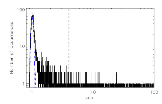
Figure 7.9 shows a histogram of $\zeta$ values throughout the season (with the basic sun, moon, and dew cuts applied). As this cut mainly correlates with 1/f noise, we only applied a very mild cut on this parameter to the data, $\zeta<4.0$. Also shown in the plot is a model of our data stream with no 1/f noise or signal of any kind. As can be seen, this distribution is sharply peaked around 1.0, with more than 99.9% of the data lying below 1.2. We tried cuts around this level, but found the cut to simply be far to sensitive at this level. At levels above 4.0, however, the cut typically correlates with our concept of bad weather, and hence this is the $\zeta$-cut level we chose. If a further analysis of the data occurs, we will most likely remove this cut in favor of something more correlated with spurious systematic effects, but for now the $\zeta$-cut is in line with our highly-demanding approach to data quality.

Outliers in the TOD

Occasionally, birds, planes, etc. would cause large short-lived spikes in the data stream. Rather than trying to identify the cause of these, we took a different tack. For each hour file and channel, we calculated the mean and standard deviation for that file, and recorded how many standard deviations the first, second, and third outliers were from the mean. Our philosophy was that any data file could have one non-Gaussian outlier, but not two. Two strong outliers were evidence of non-Gaussian behavior which would therefore not be consistent with our signal (which is at such a low level that it would not cause significant deviations from Guassinity in the data stream). Thus, we kept track of the number of standard deviations the second worst outlier was from the mean. This distribution is shown in Figure 7.10. Any HF with a more than $5\sigma$ second-worst outlier was removed. This cut accounted for $\sim$ 1.2% of the data, or about 9 hours (in addition to all previous cuts).

Figure 7.10: The distribution of second-worst outliers for each hour file. Nominal sun, moon, and dew cuts have been applied. The solid (black) curve is the J2i channel, while the dotted (blue) curve is the J2o channel. The J2i channel has large wings on both sides of the main distribution, representing non-Gaussian behavior on either side. The J2o behavior is strictly Gaussian. The vertical dashed line shows the applied cut level of $5\sigma$.

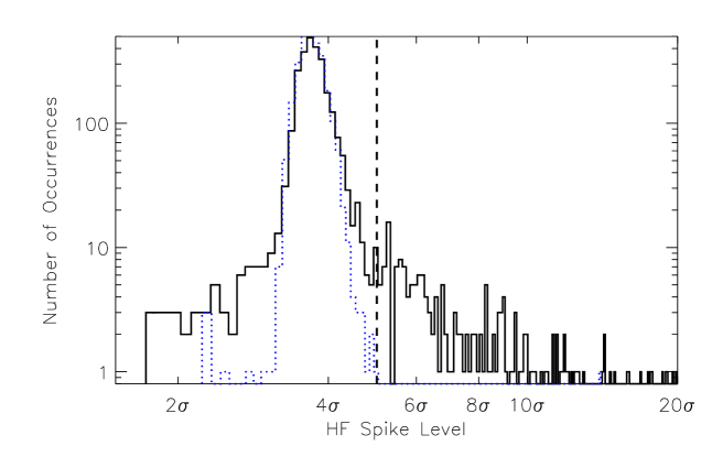
7.3.3 Duration-Based Cuts

A final series of cutting measures was based upon the length of surviving data segments. First, we required that if an HF were to survive, both its neighbors had to survive as well. Thus, if a segment of say 10 HF’s survived, the first and last of these would be chopped off. This is to ensure that the bad weather has truly ended, so this provides a nice 7.5-minute buffer. This we called the “Nearest Neighbor” cut in Table 7.1; it is a fairly common criterion in CMB data analysis.

Secondly, we required a minimum of eight (8) consecutive data files to survive in order to keep any piece of data. This is to make sure we don’t get into a situation where we’re keeping only a bunch of very short segments of data where statistically they just happened to survive the cuts, even though perhaps they were part of a larger distribution of data that should have entirely failed a given cut.

Lastly, we required a minimum of three hours total to survive a section of data. This was primarily for the offset removal step that will take place in the mapmaking part of the analysis pipeline, to be described in the next chapter. This algorithm takes place on a per-section basis, and effectively kills all information from very short sections of data; in the end we found it simpler to just remove these short sections of data.

Table 7.1 shows the sizeable effect of these duration-based cuts; together, they remove more than 10% of the full data set. However, they were quite critical; since many analysis techniques only work for long, contiguous sections of data where the noise is fairly stable, it is in our best interests to have relatively longs sections of good data. If things are changing quickly, the noise is not stable and the analysis techniques will fail.

7.3.4 Final Cuts: ROD Spikes and Executive Cuts

After we had applied these cuts to the entire data set, we were left with a set of HF’s for each channel and section. The cuts for a given QPC channel were the same as for the corresponding IPC channel. The mapmaking techniques described in the next chapter enabled us to determine a mean $Q$ and $U$ from each Hour File; this was called the ROD, or Rotation-Ordered Data set (see §8.3 for a complete description of the ROD data).

For each section and channel, we examined the distribution of these $Q$’s and $U$’s, and found there were still a fair number of outliers. We chose to proceed as in the ROD case; for any section and channel with surviving data, we found the mean and standard deviation for the $2\phi$ signal, which is $\sqrt{Q^{2}+U^{2}}$. If this quantity was more than three standard deviations from the mean for that section, we cut it. Notice that this cut is NOT independent of the other cuts; it requires a fairly clean segment of data to get meaningful, clean distributions of $Q$ and $U$ in the first place. It then finds sites of potential non-Gaussian behavior. Notice also that this cut is essentially insurance; like the $\zeta$ cut, it may easily be cutting good data, but our philosophy was “better safe than sorry” in this analysis. However, after instituting all the other cuts, this requirement only removed an additional 0.1% of the data (less than 1 hour).

At this point, there were on the order of 15 sections per channel that had some surviving data, which amounted to about 100 hours per channel. There were a couple of places where inexplicably “bad data” had survived; i.e. data with strong drifts, or a strong $2\phi$ component but no other obvious statistics indicating that anything was wrong. This latter case is entirely consistent with signal, except that the expected CMB polarization is predicted to be so low as to not be recognizable at these levels (many tens of $\mu K$). This only amounted to about two sections per channel, and again was consistent with our very restrictive cut hypothesis, so we removed them.

7.4 Final Remarks on the Cuts

It is perhaps questionable that so much of the season’s data were eliminated through the cutting process. Our aim was simply to take a very restrictive approach to the data cutting, and then loosen up these restrictions in the hope of teasing some signal from the data. Unfortunately, time constraints have prevented us from going beyond this initial step, although it is still possible in the future. The reader should keep in mind that these cuts were quite strong, so in principle there should be a minimum of spurious signals left in the data. However, even with these harshest of criteria, a spurious signal did end up residing in the data, which was only discovered through our mapmaking analysis described fully in the next chapter.

Chapter 8 From Data to Maps

Now that we have our cleaned data set, our goals are fairly clear: extract as much astrophysical and cosmological information from the data as possible. However, the data set is relatively large, on the order of $10^{8}$ numbers (about 400 MB). In the “olden days” of CMB analysis, many standard algorithms would compute cosmological parameters directly from the time-ordered data. These algorithms used techniques that needed to invert an $n\times n$ matrix, where $n$ is the number of elements in the data set. Recalling that the time it takes to invert an $n\times n$ matrix goes like $n^{3}$, we can see that these techniques will rapidly become intractable once $n$ is too great.

Luckily, it is possible to reduce a large astrophysical data set to a map of the sky, with no loss of cosmological information [131]. This perhaps surprising result lets us kill two birds with one stone: we can make maps to visualize our data, and we can radically compress our data set to make extracting cosmology from it much more tractable. In this chapter, I will describe the algorithms that take the polar data and transform it into map form. The next chapter will discuss what we can learn about astrophysics and cosmology from the maps themselves.

8.1 The General Mapmaking Problem

Many authors have written on the mapmaking problem and all the nuances that can arise during its solution. For several excellent papers on the subject, see [131, 132, 133, 134]. Most of this section is adopted directly from Max Tegmark’s excellent paper on mapmaking, reference [131].

The most intuitive and simple mapmaking algorithm is by far the “simple binning” approach, in which all data belonging to the same pixel are simply averaged together. However, drifts in the data (as from 1/f noise) can lead to stripes in the map, and also to nonsensical maps if the drifts are too strong. Thus, data belonging to the same pixel must be averaged in such a way as to remove the effect of 1/f noise. Overall offsets can also be a problem, and subtracting them in a mathematically consistent way leads to further complexities in the mapmaking algorithm. Luckily, there are well-tested algorithms that treat all the problems we will encounter.

8.1.1 Mapmaking Notation

Throughout the next sections, the mathematics of mapmaking will be discussed in great detail. Whenever discussing a vector, I will use a lowercase boldface letter (e.g. , ${\bf y}$) to represent it. Similarly, matrices will be represented by uppercase boldface letters (e.g. , ${\bf W}$). A vector such as $\tilde{{\bf x}}$ denotes our “best-guess” of the true underlying vector ${\bf x}$.

8.1.2 Definition of the Problem

The mapmaking problem proceeds as follows [131]. In general, if you have a time ordered data vector ${\bf y}=\{y_{1},\ldots,y_{n}\}$, it can be written as a sum of signal plus noise. If the signal comes from an underlying map on the sky ${\bf x}=\{x_{1},\ldots,x_{m}\}$ with $m$ pixels, then one can write

$${\bf y}={\bf A}{\bf x}+{\bf n}$$ (8.1)

where ${\bf n}$ represents the system noise, and ${\bf A}$ is called the “Pointing Matrix”, and describes how to move your data from “data space” to “map space”. The matrix ${\bf A}$ is determined entirely by the scan strategy; its evaluation is described in detail in §8.3.2. Regarding the noise ${\bf n}$, the assumption is usually made that the noise is stationary throughout the data set ${\bf y}$, which is equivalent to the power spectral density of the noise being constant in time. Under this assumption, the noise can be characterized by its noise covariance matrix, ${\bf N}$, which is defined as

$${\bf N}\equiv\langle{\bf n}{\bf n}^{t}\rangle\ ;$$ (8.2)

we assume that $\langle{\bf n}\rangle=0$ without loss of generality. For Gaussian noise, the noise covariance matrix will reduce to a multiple of the identity matrix. More complicated noise will result in correlating different measurements $y_{i}$ with each other (for instance, in the presence of 1/f noise). It is assumed that the instrumental noise is uncorrelated with the signal.

8.1.3 General Solutions to the Mapmaking Problem

Given the pointing matrix ${\bf A}$ and the noise statistics ${\bf N}$, it is straightforward to solve Equation (8.1) for the underlying map ${\bf x}$. We want to find an estimate of the map $\tilde{{\bf x}}$, given our noise (because we have incomplete, noisy data, we can’t find the exact underlying map). All linear methods can be written in the form

$$\tilde{{\bf x}}={\bf W}{\bf y},$$ (8.3)

Ideally we would like to minimize the difference between $\tilde{{\bf x}}$ and ${\bf x}$; that is, minimize $\langle|\epsilon|^{2}\rangle$ where $\epsilon\equiv\tilde{{\bf x}}-{\bf x}$. A good choice for ${\bf W}$ that essentially accomplishes this is the COBE-style solution [135, 136], which gives

$${\bf W}=[{\bf A}^{t}{\bf N}^{-1}{\bf A}]^{-1}{\bf A}^{t}{\bf N}^{-1}\ .$$ (8.4)

In general, the final map pixels in $\tilde{{\bf x}}$ will be correlated; this information is recorded in the noise covariance matrix in the map, ${\bf\Sigma}$, which is defined as

$${\bf\Sigma}\ \equiv\ \langle(\tilde{{\bf x}}-{\bf x})(\tilde{{\bf x}}-{\bf x})^{t}\rangle\ =\ {\bf W}{\bf N}{\bf W}^{t}\ .$$ (8.5)

It can be shown that, for the COBE method, this covariance matrix becomes

$${\bf\Sigma}=[{\bf A}^{t}{\bf N}^{-1}{\bf A}]^{-1}\ .$$ (8.6)

Equation (8.4) is not the only ${\bf W}$ you can choose, but it does have several nice properties [131]. It minimizes $\langle|\epsilon|^{2}\rangle$, subject to the constraint ${\bf W}{\bf A}={\bf I}$. It is the maximum-likelihood estimate of ${\bf x}$, if the underlying probability distribution for ${\bf n}$ is Gaussian [131]. And finally, the final reconstruction error $\epsilon$ is independent of the underlying map ${\bf x}$. We will hereafter refer to the mapmaking solution with this particular choice of ${\bf W}$ as Minimum Variance Mapmaking.

A couple other choices for ${\bf W}$ are noteworthy. Choosing ${\bf W}=[{\bf A}^{t}{\bf A}]^{-1}{\bf A}^{t}$, which is equivalent to ${\bf N}=\sigma^{2}{\bf I}$, is just the case of simple data averaging. As stated previously, it works well when there are no correlations between separate data points. It is easy to see physically how this works. When ${\bf W}$ acts on ${\bf y}$, the first operation (proceeding right to left) is ${\bf A}^{t}{\bf y}$, which carries your data vector into map space; it is this step that averages all data from the same pixel, and yields the unnormalized map. $[{\bf A}^{t}{\bf A}]^{-1}$ is simply the normalization factor.

If the signal covariance matrix, ${\bf S}=\langle{\bf x}{\bf x}^{t}\rangle$, is known, a Wiener-filtered version of the map can by made by choosing ${\bf W}=[{\bf S}^{-1}+{\bf A}^{t}{\bf N}^{-1}{\bf A}]^{-1}{\bf A}^{t}{\bf N}^{-1}$ [137, 138]. A Wiener-filtered map is typically used for visual presentation of maps, as it is less noisy (at the price of introducing additional pixel-pixel correlations). This technique also has the property of minimizing $\langle|\epsilon|^{2}\rangle$. It can be shown that the Wiener-filtered map, taken together with its noise covariance matrix ${\bf\Sigma}$, contains identical information to the Minimum Variance Mapmaking-derived map.

Overall, the linear method (based on Equation (8.3)) is extremely general, and can be applied to any type of problem where a linear combination of data is made in order to determine some physical parameter. Whenever the noise of said data isn’t white, this is the best approach. For polar, we will exploit this technique no fewer than four different times throughout the analysis pipeline. However, this method breaks down when the noise is not stable, so the trick is to apply the technique to short “chunks” of data, where the noise was stable, and then piece all these submaps together at the end. It will turn out that the same mapmaking trick will also tell us how to do this.

8.2 Mapmaking for POLAR

8.2.1 The POLAR Pixelization

Let us now lay out the details of the mapmaking problem for the case of polar. We would like to construct maps of both $Q$ and $U$; because of our scan strategy, a zenith drift scan at $\delta=43^{\circ}$, this will be a 1D map in right ascension. We can choose to pixelize this however we like, but will lose information if the pixels we choose are too big. As we have a 7^∘ beam (FWHM), the number of independent pixels is $\frac{360}{7}\cos{43^{\circ}}\sim 38$. We lose nothing in choosing smaller pixels, because we can always average them together to form larger pixels later, but you can lose information if your pixel size is too large. The rule of thumb is to pixelize at $\sim$ 40% of your beam FWHM or smaller.

For polar, we chose to use 180, 2^∘ RA-pixels, with the first pixel arbitrarily centered at RA = 0^∘. These were large enough so that there weren’t a ridiculous number of them (the more pixels there are, the harder the final likelihood analysis becomes), and small enough not to lose any potential information.

8.2.2 Overview of POLAR’s Analysis Pipeline

We would like to obtain maps of $Q$ and $U$ for each of our three polarization channels (26–29, 29–32, and 32–36 GHz). If frequency-dependent foregrounds do not prove to be a problem, we can then average the maps of the three channels into final overall maps of $Q$ and $U$, and proceed to do cosmology with those maps.

Figure 8.1: Flow Chart of the POLAR Data Analysis Pipeline

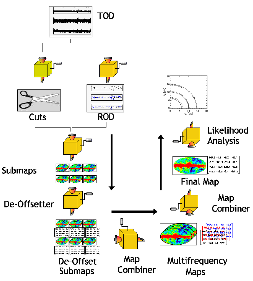
Figure 8.1 gives an overview of the entire analysis pipeline. We begin with the calibrated data time stream, which we refer to as the Time–Ordered Data, or “TOD”. Instead of simply going straight from $TOD\rightarrow Maps$, we will make a couple of intermediate “rest stops” to simplify the problem. The primary intermediary we call the Rotation–Ordered Data, or “ROD”. The ROD is the projection of the $1\phi$ and $2\phi$ components from the data set (effectively, a time stream of $Q$’s and $U$’s); its construction is described in §8.3. For all sections of data passing the cuts, we form “submaps” of $Q$ and $U$ (see §8.4). For example, if one day we observed for seven hours of clear weather, we would obtain submaps for $Q$ and $U$, for each channel, each $\sim$ 53 pixels long (given the above pixelization). When we do this for all sections of data, we will arrive at some number of submaps. See the glossary, Appendix A, for additional clarification of these terms.

Unfortunately, during the analysis we discovered that the ROD data itself had unforeseen offsets at the level of hundreds of $\mu K$. These were offsets in the parameters $Q$ and $U$ themselves, to be distinguished from the overall offsets $I_{0}$ in each channel; these offsets are discussed in great detail in §8.5. This new problem necessitated an additional step to remove the offsets(see §8.6), forming “de-offset submaps”. We then combine these de-offset submaps into final maps for $Q$ and $U$ for each channel (§8.7), and taking into account the inter-channel correlations, combine these channel maps into final maps for $Q$ and $U$ (§8.7.4).

8.3 Rotation-Ordered Data (ROD)

To form the ROD, we must robustly extract the coefficients of the simple Fourier expansion of the time-ordered data. If y(t) is some segment of the TOD, then

$$y(t_{i})\;=\;I_{0}+c_{i}\cos{\phi_{i}}+s_{i}\sin{\phi_{i}}+q_{i}\cos{2\phi_{i}}+u_{i}\sin{2\phi_{i}}+n(t)\quad;$$ (8.7)

this is the signal seen at time $t_{i}$ (the i^th sample), when the polarimeter is at a rotation angle of $\phi_{i}=\omega t_{i}$ with respect to geographic North, and $n(t)$ denotes the noise. The coefficients $\{c,s,q,u\}_{i}$ are lower-case to denote they are elements of vectors, and will hereafter be referred to as the Rotational Coefficients. The term “ROD” will hereafter refer to this time series of rotational coefficients. $I_{0}$ is the overall DC level, and is not used in the analysis.

We choose to extract these coefficients once per hour file, due to our stationarity assumption. We could have chosen to extract the coefficients for each individual rotation, but one rotation covers only about 0.13^∘ on the sky, whereas our beam size is 7^∘. It is to our benefit to average more, since our beam smears out all information at scales much below our beam size. The hour-file standard is a nice compromise between having a section too short (less compression), and too long (difficult to compute the rotational coefficients, and failure of noise stationarity assumption).

8.3.1 The Simple Approach to ROD extraction

The most straightforward way to form the ROD data is simply to “project out” the components we are interested in by using the orthogonality of sines and cosines. For a data vector ${\bf y}$ from a single hour file with $N_{f}$ elements, $q$ and $u$ are given by

$$q\ =\ \frac{2}{N_{f}}\sum_{i=1}^{N_{f}}y_{i}\cos{\phi_{i}}$$ (8.8)

$$u\ =\ \frac{2}{N_{f}}\sum_{i=1}^{N_{f}}y_{i}\sin{\phi_{i}}$$ (8.9)

where $\phi_{i}$ is the polarimeter rotation angle at sample $i$. Although it is very simple and fast, this approach has two important drawbacks. First, it ignores the effects of 1/f noise in our data. Because the noise from our polarization channels is almost always flat, 1/f noise will play a small role, but in order to get a good estimation of our errors, it is important to know the contribution to the errors from this noise component.

The second drawback to this simple projection method is that it ignores our pixelization scheme, described in §8.2.1. An hour file spans 1.875^∘ in Right Ascension, while our chosen pixel size on the sky spans 2^∘; these are fairly well-matched, but not perfectly, and they will not always line up. There could easily be an hour file that straddles two sky pixels equally. This is most likely a small effect, but it is easy to treat exactly, using the formalism of Minimum Variance Mapmaking as discussed in the next section.

8.3.2 ROD Extraction Using Minimum Variance Mapmaking

To this end, we seek to discern which sky pixels a given data file spans (for this pixelization it is 1 or 2 only); then we must determine the rotational coefficients implied by the data file for each of these pixels. Couple this to the 1/f noise effect and it seems a pretty daunting task, but the amazing thing is that Minimum Variance Mapmaking covers it all!

To use this technique, we need our data vector ${\bf y}$, our noise covariance matrix ${\bf N}$, and the pointing matrix ${\bf A}$. We obviously know y, but keep in mind that we do one of these operations for each channel (including the QPC for completeness). Next we show how to calculate the ${\bf N}$ and ${\bf A}$ matrices.

The Pointing Matrix

${\bf A}$ is the transformation matrix that maps the sky map into our data stream; it depends only on the scan strategy and beam parameters. ${\bf A}$ has a number of columns equal to the number of map pixels and a number of rows equal to the number of data samples.

The case of assembling ${\bf A}$ for a one-horn total power experiment is particularly easy. For each row, you simply put a ‘1’ in the column of the pixel that this particular sample came from, and zeros everywhere else. Thus, ${\bf A}$ is an exceedingly sparse matrix made up of 1’s and 0’s in the total power (intensity) case, such as most anisotropy experiments. A good example of this is given in [136], where the case of multiple horns is also treated.

Because of polar’s rotation and the fact that we are observing the Stokes parameters $Q$ and $U$, our situation is somewhat more complicated. Let us write the map vector as ${\bf x}=\{{\bf c},{\bf s},{\bf q},{\bf u}\}$. At some time $t_{i}$, the signal we observe is given by Equation (8.7). Now it is straightforward to form the pointing matrix ${\bf A}$, so that Equation (8.1) holds. Let us consider a toy model in which there are four sky pixels spanned by the data segment we are analyzing. Our map in this case is a 16-element vector, containing the four rotational coefficients for each of the four pixels . For the observations ${\bf y}$ within the data segment, a sample pointing matrix would look like the following (I show ${\bf A}^{t}$ for simplicity):

$${\bf A}^{t}=\left(\begin{array}[]{cccccccccc}0&0&\ldots&0&0&\ldots&0&0&\ldots&0\\ \cos{\phi_{1}}&\cos{\phi_{2}}&\ldots&\cos{\phi_{a}}&0&\ldots&0&0&\ldots&0\\ 0&0&\ldots&0&\cos{\phi_{a+1}}&\ldots&\cos{\phi_{b}}&0&\ldots&0\\ 0&0&\ldots&0&0&\ldots&0&\cos{\phi_{b+1}}&\ldots&\cos{\phi_{N_{f}}}\\ \hline\cr\vspace{-5mm}\hfil\\ 0&0&\ldots&0&0&\ldots&0&0&\ldots&0\\ \sin{\phi_{1}}&\sin{\phi_{2}}&\ldots&\sin{\phi_{a}}&0&\ldots&0&0&\ldots&0\\ 0&0&\ldots&0&\sin{\phi_{a+1}}&\ldots&\sin{\phi_{b}}&0&\ldots&0\\ 0&0&\ldots&0&0&\ldots&0&\sin{\phi_{b+1}}&\ldots&\sin{\phi_{N_{f}}}\\ \hline\cr\vspace{-5mm}\hfil\\ 0&0&\ldots&0&0&\ldots&0&0&\ldots&0\\ \cos{2\phi_{1}}&\cos{2\phi_{2}}&\ldots&\cos{2\phi_{a}}&0&\ldots&0&0&\ldots&0\\ 0&0&\ldots&0&\cos{2\phi_{a+1}}&\ldots&\cos{2\phi_{b}}&0&\ldots&0\\ 0&0&\ldots&0&0&\ldots&0&\cos{2\phi_{b+1}}&\ldots&\cos{2\phi_{N_{f}}}\\ \hline\cr\vspace{-5mm}\hfil\\ 0&0&\ldots&0&0&\ldots&0&0&\ldots&0\\ \sin{2\phi_{1}}&\sin{2\phi_{2}}&\ldots&\sin{2\phi_{a}}&0&\ldots&0&0&\ldots&0\\ 0&0&\ldots&0&\sin{2\phi_{a+1}}&\ldots&\sin{2\phi_{b}}&0&\ldots&0\\ 0&0&\ldots&0&0&\ldots&0&\sin{2\phi_{b+1}}&\ldots&\sin{2\phi_{N_{f}}}\\ \end{array}\right)\vspace{3mm}$$ (8.10)

In this example, for observations $t_{a}$ through $t_{b}$, we were aimed at pixel 2, and likewise pixel 3 corresponds to $t_{b}+1$–$t_{c}$, and pixel 4 to $t_{c}+1$–$t_{d}$. I included pixel 1 here to show that we are not penalized for keeping extra pixels that don’t have any data; they simply get all 0’s in ${\bf A}$, and will have infinite error bars in the final map. Then, by multiplying any row in ${\bf A}$ (any column in ${\bf A}^{t}$) by the map vector ${\bf x}$, we recover Equation (8.7) in the absence of noise (and with no DC level), which was our original goal.

Noise Covariance Matrix Construction for ROD extraction

In order for this machinery to work we must adequately understand our noise, in the form of its noise covariance matrix ${\bf N}$. For our data files (HF’s), this will be a $9000\times 9000$ symmetric, positive-definite matrix ($N_{f}=9000$ samples per data file). It has the special property that each row equals the row above it, right-shifted by one element (with wrap-around boundary conditions). Thus, instead of containing $N_{f}^{2}$ pieces of information, in this special case of noise stationarity, the data covariance matrix contains only $N_{f}$ independent numbers.

In order to characterize ${\bf N}$, as I will show below, all we really need to know is the power spectrum of the noise. A reasonable estimate of the PSD is obtained by using only the data from this file; however, with this method the PSD comes from a mere $N_{f}=9000$ numbers and is very noisy at low frequencies, precisely where we most need to know its shape. We therefore perform a fit of the PSD to the following model :

$$S(\nu)=\sigma^{2}(1+\frac{\nu_{knee}}{\nu})\qquad[K^{2}\ Hz^{-1}]\ ;$$ (8.11)

this is simply the case of white plus 1/f noise, where the knee frequency is $\nu_{knee}$. There is also a 5 Hz low-pass filter on our data, which correlates samples taken within about 0.2 seconds of each other (or about every four samples). However, this is irrelevant because all our information is contained at much lower frequencies, $\sim$ 0.067 Hz, where the filter response is effectively unity, and so we leave it out of our noise model.

Algorithmic Tricks for ROD Extraction

Let us return to the algorithm at hand, which to remind the reader, is

$$\tilde{{\bf x}} = [{\bf A}^{t}{\bf N}^{-1}{\bf A}]^{-1}{\bf A}^{t}{\bf N}^{-1}{\bf y}$$ (8.12a)

$${\bf\Sigma} = [{\bf A}^{t}{\bf N}^{-1}{\bf A}]^{-1}$$ (8.12b)

where $\tilde{{\bf x}}$ are our rotational coefficients for a particular 7.5 minute data file, and the algorithm for ${\bf A}$ was given above. As we will need to perform this algorithm for each channel and each hour file, that is, about $6\times 800\simeq 5000$ times, we would like it to be as fast as possible. ${\bf N}$ may not seem large, but inverting a $9000\times 9000$ matrix 5000 times takes a while on any computer. And we haven’t even fully evaluated ${\bf N}$ yet, only its power spectral density.

The algorithm becomes more numerically palatable by making the following definitions:

$${\bf y}_{e}\ =\ {\bf N}^{-1/2}{\bf y}$$ (8.13a)

$${\bf A}_{e}\ =\ {\bf N}^{-1/2}{\bf A}$$ (8.13b)

in which case $\tilde{{\bf x}}$ and ${\bf\Sigma}$ simplify to

$$\tilde{{\bf x}} = [{\bf A}_{e}^{t}{\bf A}_{e}]^{-1}{\bf A}_{e}^{t}{\bf y}_{e}$$ (8.14a)

$${\bf\Sigma} = [{\bf A}_{e}^{t}{\bf A}_{e}]^{-1}$$ (8.14b)

The reason this is numerically better than Equation (8.12) is that there is a fast way to calculate ${\bf y}_{e}$ and ${\bf A}_{e}$. Rather than work in the time domain, we can work in the Fourier domain, where we can use the Fast Fourier Transform (for example, see Numerical Recipes Chapter 12 [111]) to great advantage.

Instead of constructing ${\bf N}$, we simply work with the PSD of N (this has units of $K/\sqrt{Hz}$), which we denote as $S_{N}(\nu)$. Using Fourier tricks, Equation (8.13) becomes

$${\bf y}_{e}\ =\ \mathcal{F}^{-1}\{\,\frac{\mathcal{F}\{{\bf y}\}}{S_{N}(\nu)}\,\}$$ (8.15a)

$${\bf A}_{e}^{i}\ =\ \mathcal{F}^{-1}\{\,\frac{\mathcal{F}\{{\bf A}^{i}\}}{S_{N}(\nu)}\,\}\ ,$$ (8.15b)

where ${\bf A}^{i}$ is the $i^{th}$ row of ${\bf A}$, and “$\mathcal{F}$” denotes the Fourier Transform. So we’ve reduced the algorithm to a bunch of FFT’s, which are quite fast and make the computation very manageable on almost any workstation.

Figure 8.2: Effect of Prewhitening on sample noise PSD. Panel (a): PSD for a sample Hour File, with a knee frequency of $\sim$ 0.03 Hz, a high but not unreasonable value. The solid (blue) curve is the logarithmic-weighted fit to the PSD. The vertical dashed lines show the $1\phi$ and $2\phi$ rotational frequencies. Panel (b): Same as (a), but for the ${\bf y}_{e}$ version of the data. The effect was to whiten the low-frequency section of the PSD; it is equivalent to dividing the PSD by the fitted curve. Note that the roll-off due to the anti-aliasing filter remains untouched.

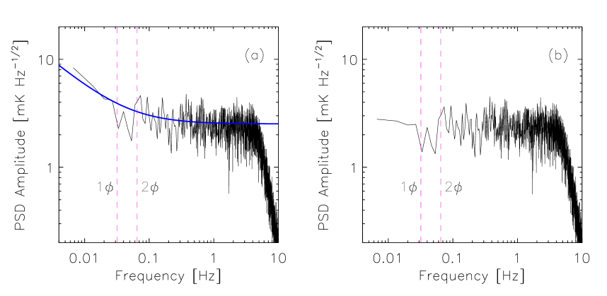
However, Equations 8.13 have physical meaning as well. Turn your attention to Figure 8.2; the figure displays the PSD amplitude of one short section of data. It shows the action of ${\bf N}^{-1/2}$ as a “pre-whitening filter” on ${\bf y}$; that is, the effect is that the low-frequency 1/f rise in the PSD is fitted for and removed.

Figure 8.3: Effect of ${\bf N}^{-1/2}$ on a column of the Pointing matrix ${\bf A}$. The black (solid) curve shows a section of the U-column of a sample pointing matrix. The blue curve shows the same column from the effective pointing matrix ${\bf A}_{e}$, processed according to Equation (8.15b), with a knee frequency of 0.01 Hz (about 1/6 of the $2\phi$ frequency shown here). Notice that some of the response has been smoothed out to the left, where the original response was zero, at the price of lowering the primary pixel response.

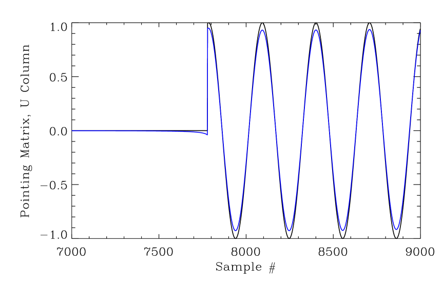
The effect on the pointing matrix ${\bf A}$ is also interesting. Figure 8.3 shows a section of one column of ${\bf A}$, a column that extracts $U$ for a certain pixel. With a knee frequency of 0.01 Hz (about 1/6 of the $2\phi$ frequency), you can see the slight difference between ${\bf A}$ and ${\bf A}_{e}$. The pixel we want sensitivity to comes into view about sample number 7800. However, some “power” is removed from this main pixel, and there is some leakage from the previously-viewed pixel to the desired one due to the presence of 1/f noise.

At this point, the reader may ask him/herself if such “processing of the data” is warranted. Let me be clear about this: Minimum Variance Mapmaking as I have defined it yields the best map in the sense that it has minimum variance while retaining all the cosmological information [140]. There will be some correlation between pixels manifested in off-diagonal elements of the map covariance matrix. Thus, there is no cheating involved; we are not prewhitening the data and then constructing maps. Rather, in the process of constructing maps, a prewhitened version of the data arises naturally, but because we also modify the pointing matrix (${\bf A}\rightarrow{\bf A}_{e}$), we are not throwing away any information.

8.3.3 First Peek at the ROD: Offsets revealed

We perform the above algorithm on all HF’s, even those that didn’t survive data quality checks; we institute those in the next step (see Figure 8.1). Thus, we now have a new data set, the so-called ROD data, which again are the $Q,U$ rotational coefficients on the sky for each HF. However, another useful data set to construct is one which is identical to ROD except that precisely one set of rotational coefficients (that is, {c,s,q,u}) is determined for each HF (rather than tagging them to specific sky pixels). Because data from consecutive rotations are averaged together, this data set lets us see the characteristics of the ROD data more directly. In the following analysis of the timestream of rotational coefficients and other related quantities, it is this latter data set that was used.

Figure 8.4: The mean values of $Q$ and $U$ for the ROD data set versus time; each data point represents one Hour File. Non-Gaussian behavior is immediately apparent at the 50-100 $\mu K$ level.

Figure 8.5: Same as Figure 8.4 but for the QPC channels. There is no evidence of any offsets from these distributions in the QPC channels, eliminating any sort of electrical cause of the offsets.

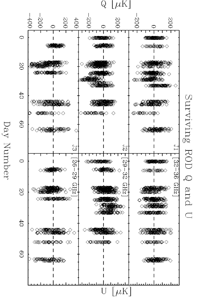
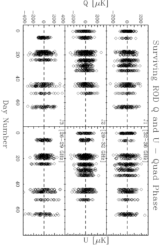
Figure 8.4 shows the derived $Q$ and $U$ values for all the surviving data for the three primary IPC polarization channels, while Figure 8.5 shows this same information for the QPC channels. Notice that the data lie in “chunks” along the time axis; this is because the surviving data were in sections 3-12 hours long each (there were about 20 of them); we call these surviving chunks simply “sections”, and the maps on the sky corresponding to each one we call a “submap” (see glossary).

The primary feature of these graphs is the changing offset level of each section of data, present for the in-phase (IPC) channels, but not seen in the quadrature (QPC) channels; i.e., the IPC channels are obviously not consistent with purely Gaussian noise. From these plots alone, it is difficult to discern what the nature of the apparent signal is, but it is obvious that it is a global issue in our data that may strongly affect our results. Hereafter we refer to these apparent signals as “offsets”, for lack of a better description. In §8.5 we will examine the offset issue in more detail.

8.4 From ROD to Submaps: How to Add Maps

At this point in the data pipeline we find ourself with the ROD data: a time stream of rotational coefficients, each tagged to a particular pixel on the sky. For each HF, we have a “mini-map” of just one or two sky pixels, and determine what the Stokes’ parameters are for each of these one or two pixels, and also determine the covariance matrix between these two pixels and all the calculated parameters. We do things on the level of the HF for calculational convenience, and to ensure that our noise stationarity assumption is valid.

Now we work our way up the “time-scale” ladder: for each section of data, we combine all the little 1–2 pixel HF maps together into one map for each channel, and calculate its corresponding covariance matrix; these are our submaps. We find robustly that the “inter-coefficient correlations”, that is, offsets between $Q$ and $U$ and the like within a pixel, were completely negligible. We forget about our $C$ and $S$ data at this point; these coefficients do contain information on systematic effects, but making maps from them will be difficult to interpret and hence not be particularly informative.

We are hence faced with the standard “map combination” problem: given a collection of $m$ maps $\{{\bf x}_{1}\ldots{\bf x}_{m}\}$ with corresponding covariance matrices $\{{\bf N}_{1}\ldots{\bf N}_{m}\}$, what is the best estimate of the full map? The problem is complicated by the fact that our maps are incomplete – each only covers a part of the total map.

Let us deal with the latter problem first. The solution to partial sky coverage is to “expand” each initial map to cover the final map by making up values for the unmeasured map pixels, but giving those values zero weight by assigning them infinite uncertainty in the noise covariance matrix. As an example, let us say one of our initial maps measures pixels 2 and 3 of a four-pixel map. We perform the following “expansion of this initial map”:

$${\bf x}_{i}\ =\ \{x_{2},x_{3}\}\ \rightarrow\ \{0,x_{2},x_{3},0\}$$ (8.16)

and

$${\bf N}_{i} = \left[\begin{array}[]{cc}N_{11}&N_{12}\\ N_{21}&N_{22}\end{array}\right]\rightarrow\ \left[\begin{array}[]{cccc}\infty&0&0&0\\ 0&N_{11}&N_{12}&0\\ 0&N_{21}&N_{22}&0\\ 0&0&0&\infty\end{array}\right]$$ (8.17g)

and $$\qquad\qquad{\bf N}_{i}^{-1}\ \rightarrow\ \left[\begin{array}[]{cccc}0&0&0&0\\ 0&N^{-1}_{11}&N^{-1}_{12}&0\\ 0&N^{-1}_{21}&N^{-1}_{22}&0\\ 0&0&0&0\end{array}\right]$$ (8.17l)

We see it is a trivial task to deal with the partial sky coverage problem. I show the inverse covariance matrix because that is what is actually used in the formalism.

Now let us assume that our maps $\{{\bf x}_{1}\ldots{\bf x}_{m}\}$ and covariance matrices $\{{\bf N}_{1}\ldots{\bf N}_{m}\}$ have been expanded to all have equal coverage. How do we then find the most-likely/minimum noise map containing all the information? The answer is, of course, Minimum Variance Mapmaking! We simply take our data vector to be ${\bf y}\ =\ \{{\bf x}_{1}\ldots{\bf x}_{m}\}$, and we make a block-diagonal “mega-covariance matrix” ${\bf N}$ with all the little ${\bf N}_{i}$’s on the diagonal. Since we’ve expanded each ${\bf x}_{i}$ map to have the same pixel coverage as the final map we’re pointing to, each has a “pointing matrix“ that is simply the $n$-element identity (assuming the maps all have $n$ pixels). The full pointing matrix is then ${\bf A}=[{\bf I},\ldots,{\bf I}]$, so A is a $(nm)\times n$ rectangular matrix. Applying the standard Minimum Variance Mapmaking formalism, Equations 8.3–8.4, the final map is

$${\bf x}_{f} = [{\bf A}^{t}{\bf N}^{-1}{\bf A}]^{-1}{\bf A}^{t}{\bf N}^{-1}{\bf y}$$ (8.21)

$$= \left[\sum_{i=1}^{m}{\bf N}_{i}^{-1}\right]^{-1}[{\bf N}_{1}^{-1},\ldots,{\bf N}_{m}^{-1}]\left[\begin{array}[]{c}{\bf x}_{1}\\ \vdots\\ {\bf x}_{m}\end{array}\right]$$

Then the final map ${\bf x}_{f}$ and final covariance matrix ${\bf N}_{f}$ are given by

$${\bf N}_{f}\ =\ \left[\sum_{i=1}^{m}{\bf N}_{i}^{-1}\right]^{-1}$$ (8.22a)

$${\bf x}_{f}\ =\ {\bf N}_{f}\ \left[\sum_{i=1}^{m}{\bf N}_{i}^{-1}\ {\bf x}_{i}\right]$$ (8.22b)

which is the standard result (e.g. , [133, 141]).

We applied this technique to all the data passing our cuts, in order to make a submap for each section, channel and {Q or U} combination, for both the IPC and QPC channels: this generates approximately $6\times 20\times 2=240$ submaps on the sky. As will be discussed in the next section, the offset that was noticed in the ROD data is even more apparent once these submaps are formed; the offset problem and how we dealt with it are discussed in the next two sections.

8.5 Characterizing the ROD Offsets

Figure 8.6: Q and U offsets binned by section, for all six polarization channels. The (black) triangles correspond to the $Q$ offsets, while the (blue) squares correspond to the $U$ offsets. The channels are indicated in the upper left-hand corner of each plot. The displayed error bars are statistical. Only data that survived the quality cuts contributed to this plot.

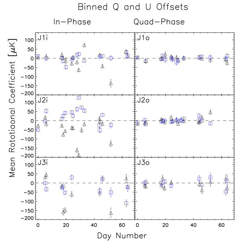
Let us now return to the issue of the ROD “offsets” discussed previously. Perhaps the first logical question to ask is, just how statistically significant are these offsets? Figure 8.6 shows the offsets in $Q$ and $U$ for all six channels as a function of time, but averaged down to a single number per section, with the corresponding derived statistical error. As you can see the effect is strong (multi-sigma) and quite variable, an experimentalist’s worst nightmare.

Based on this plot, we can already give some qualitative characteristics of the offsets. First, there is no visible effect for the QPC channels, eliminating some kind of electrical explanation. It seems that the effect is sometimes correlated among the three channels, but not always. If there were always a strong correlation among the channels, we could probably attribute the effect to some specific optical phenomenon, such as sidelobe pickup of the 300 K earth. But its time-varying nature makes it difficult to ascribe a particular cause to it.

Figure 8.7: $2\phi$ Offset Angles for each of the three IPC channels during the season. For a given section, the $2\phi$ offset angle is defined as $\arctan{\frac{\langle U\rangle}{\langle Q\rangle}}$. The stars, triangles, and squares, correspond to channels J1i, J2i and J3i, respectively. Standard error propagation is used to derive errors on the angle from the errors on $\langle Q\rangle$ and $\langle U\rangle$. Data cuts used are slightly less restrictive than the standard cuts, in order to enable direct comparison between the three IPC channels.

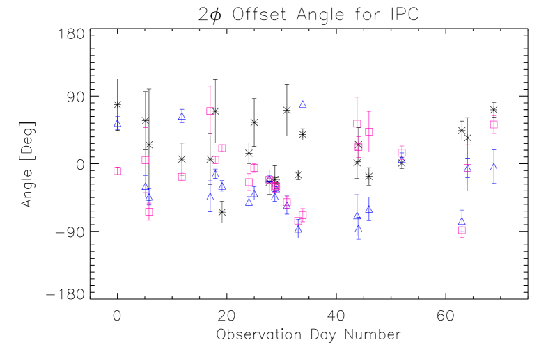
A final interesting quantity to look at is the relationship between $Q$ and $U$. Specifically, let us define the $2\phi$ offset angle as $\arctan{\frac{\langle U\rangle}{\langle Q\rangle}}$. In Figure 8.7, this quantity is calculated for each submap as in Figure 8.6, but a slightly less restrictive cut has been used that cuts on our three channels equally. Corresponding error bars on the angles are derived. First, notice that the errors on J1i’s angle are quite high, indicating that it doesn’t have a strong offset problem. J2i’s offset angle is relatively stable, especially for a long period in the middle of the season. J3i’s offset is less stable. However, there is a telling correlation between all three channels that implies a possible common origin. Similar results are obtained for the $1\phi$ coefficients $C$ and $S$ and the resulting angle; J1i shows small offset angles, J2i shows a fairly stable offset angle, and all three channels exhibit some correlation.

8.5.1 A Possible Sky Signal?

Is the effect consistent with some type of signal attached to the sky? It is far too strong to be CMB polarization, but it is conceivable that the structure is due to strong synchrotron or spinning dust. Figure 8.8 shows the same data again for channel J2i (which exhibits particularly strong “offsets”), plotted in right ascension. Polynomials of varying degree were fit to each submap, as described in the figure caption. Clearly, there is nothing visibly consistent with a true sky signal. Certain submaps are totally inconsistent with other submaps covering the same section of sky. The same conclusion holds true for the other polarization channels as well.

Figure 8.8: Polynomial fits to J2i offsets, plotted in right ascension. Polynomials of varying degree were fit to each submap; for submaps with less than four hours of data, a line was fit to the data, while a quadratic was fit to submaps with more than four hours of data. Different sections are indicated by different colors.

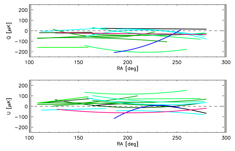
8.5.2 Rotation-Synchronous Analysis

It is quite useful to take a step back at this point, and form a “map” straight from the time-ordered-data that is binned into coordinates fixed to the ground rather than to the sky. Offsets in $Q$ and $U$ can only come from signals that are synchronous with our rotation frequency (specifically, at its first harmonic); these offsets are naturally due to a rotation-synchronous noise component.

Figure 8.9: Correlator time streams plotted in ground-based coordinates, for the night of May 5, 2000. Only data passing the quality cuts are shown. The left three panels show the overall polarimeter response as a function of angle; it is quite stable considering the large (tens of mK) offset on each channel. The right three panels show the same information with the offsets removed; the solid line shows the best-fit curve including both $1\phi$ and $2\phi$ frequencies.

Figure 8.10: Correlator time streams plotted in ground-based coordinates for the night of March 28, 2000. Plot conventions are the same as Figure 8.9. This plot shows a striking lack of rotation-modulated systematics. In general, the $C$, $S$, $Q$, and $U$ offsets varied quite a bit throughout the season, as discussed in the text.

Rotation-synchronous plots are made of two sections of data in Figures 8.9 and 8.10. The first figure shows this information for the three IPC channels from a particular night of good data. The panels on the left of the figure are simply to remind the reader of the large offsets upon which the rotation-synchronous signals ride. These “$I_{0}$” offsets are typically 10–100 mK (see Figure 8.6), and are due to the cross-polarization of the OMT. The right-hand panels show the same plots with $I_{0}$ removed; it is evident that there is a strong rotation-synchronous effect (100-200 $\mu K$), correlated among the three channels.

However, it was not always this way. Figure 8.10 shows a night of data from earlier in the season where the synchronous effect was significantly smaller, though not negligible. In this example, J1i and J2i appear somewhat correlated, but J3i doesn’t exhibit signs of visible contamination. The fact the that overall offsets were significantly lower in this case is somewhat misleading; there are cases throughout the season when the TOD offsets were high and the ROD offsets were low, and vice versa (and, indeed, everything in between).

8.5.3 Conjectures on the Rotation Synchronous Effect

It is worthwhile to speculate on the cause of these rotation-synchronous offsets, although let me be clear from the outset that ultimately we never identified the culprit(s). For reference, here are some specific facts on the rotation-synchronous offsets:

• The offsets were often strongly correlated among channels, especially when the offsets were strong.

• There was marked anti-correlation between Q and U, especially in channel J2i.

• J1i had the weakest offset, with almost no visible effect on U.

• Offsets were highly variable throughout the season, although for J1i and J2i typically $Q$ was negative and $U$ was positive.

• There was a degree of correlation in the offset angles ($\arctan{\frac{\langle U\rangle}{\langle Q\rangle}}$) between the three IPC channels.

• No offsets are visible in the QPC channels.

8.5.4 Asymmetric Beam Shape+Anistropic Sky

So, what could this mystery effect be? A real possibility is atmospheric emission, coupled with an asymmetric beam pattern. Recall that $I_{0}$, the TOD offset in the polarization channels, can be coupled into the radiometer via non-zero cross-polarization of the OMT. If we have a symmetric beam shape, as polar rotates, you should get the same offset. However, if our beam has a $2\phi$ component, this will cause the offset to similarly be modulated at this level. As $I_{0}$ varies with atmospheric and ground-based variables, such as temperature and precipitable water vapor, it is easy to see how this could enter in.

8.5.5 Outer Ground Screen Pick-Up

Another possibility is associated with the outer ground screens. While the inner conical ground screen rotates with the experiment, the outer ground screens are fixed (see §4.4.6). The outer screens have a natural quadrupolar component, being composed of four large aluminum panels. The sky will reflect off of these panels and enter our sidelobes, and at some level there will be a natural quadupolar component to this contamination. Again, it will vary throughout the season as the atmospheric emission varies. The frequency dependence will be a complicated interplay of the frequency-dependent features of the horn, OMT, ground-screens and atmosphere.

8.6 Offset Removal Techniques

Whatever the ultimate cause of the offsets, it is clear we must do something about them in order to proceed with the data analysis. If we had some model of the effects that could make successful predictions about its level, we could use it to safely subtract out the offsets without strongly affecting our signal recovery. However, without such a model we must proceed along a different path, which assumes no knowledge of the offset cause.

Most experiments have offsets that they must deal with, although ours is particularly insidious because it is so variable. Luckily, machinery has been developed to account for this contingency. A literature search reveals that the topic was apparently first addressed by Rybicki and Press [142, 143]. The QMAP group introduced the method of “virtual pixels” (sometimes called “extra pixels”) to estimate and remove offsets, see [133]. Max Tegmark derived tricks for the removal of unwanted modes in CMB maps in [132], although the techniques are quite general. Bond, Jaffe, and Knox introduced the method of marginalization, where unwanted modes of a time stream or map have infinite noise added to them, thus removing them [134] (hereafter BJK). Recently, the DASI group used the BJK technique to deal with their offset problems [20], while the MAXIMA group explored both extra pixels and marginalization, and provide a great review of these techniques in their excellent mapmaking paper [141].

Although the mechanics of the two primary mode-removal techniques, the Tegmark-QMAP technique of extra pixels and the BJK/Tegmark technique of marginalization, are quite different, they produce identical results. Typically one or the other is more convenient, depending on the situation. We will briefly explore each of these methods below; our discussion draws heavily upon [141], to which the reader is referred if more details are required.

8.6.1 Direct Offset Removal

Let us first define our problem. Consider a data vector ${\bf y}$ and corresponding noise covariance matrix ${\bf M}$. ${\bf y}$ may correspond to a map, submap, or to time-ordered data; it doesn’t matter. First, what is the offset in ${\bf y}$ – that is, what is its weighted mean? The easiest way to calculate this is using Minimum Variance Mapmaking again, but taking your output “map” to be a single number! Using this approach it can be shown that for a piece of data ${\bf y}$ with noise covariance ${\bf N}$, the weighted mean is given by

$$\langle{\bf y}\rangle=[{\bf e_{0}}^{t}{\bf N}^{-1}{\bf e_{0}}]^{-1}{\bf e_{0}}^{t}{\bf N}^{-1}\,{\bf y}]$$ (8.23)

where ${\bf e_{0}}$ is a column vector of all 1’s. Notice that ${\bf e_{0}}$ is our pointing matrix in this case – it “points” to only one pixel, the mean. Similarly, the data with the mean removed is given by

$${\bf y}-\langle{\bf y}\rangle = \ {\bf\Pi}\ {\bf y}$$ (8.24a)

$${\bf\Pi} \equiv {\bf I}-{\bf e_{0}}[{\bf e_{0}}^{t}{\bf N}^{-1}{\bf e_{0}}]^{-1}{\bf e_{0}}^{t}{\bf N}^{-1}$$ (8.24b)

I have intentionally expressed this relation as some matrix ${\bf\Pi}$ operating on our data vector; it is inordinately handy to use an operator that extracts the weighted mean of something, and have that operator be independent of the data itself (it only depends on the noise properties of the data). Note that ${\bf\Pi}$ is not in general symmetric. Now, the covariance matrix of our new data set ${\bf y}-\langle{\bf y}\rangle$ can be easily calculated:

$${\bf C}\ \equiv\ ({\bf y}-\langle{\bf y}\rangle)({\bf y}-\langle{\bf y}\rangle)^{t}\ =\ {\bf\Pi}\ {\bf N}\ {\bf\Pi}^{t}\ =\ {\bf\Pi}\ {\bf N}\ =\ {\bf N}\ {\bf\Pi}^{t}$$ (8.25)

where the final two equalities are easily shown given the definition of ${\bf\Pi}$ given in Equation (8.24).

It turns out that ${\bf C}$ is singular; this is a direct property of the fact that we have lost sensitivity to the mean of ${\bf y}$, which indirectly leads to a zero eigenvalue in ${\bf C}$ for this technique. However, for the purposes of a likelihood analysis, all we will need is the “pseudo-inverse” of ${\bf C}$, which we denote as ${\bf\mathcal{C}}^{-1}$:

$${\bf\mathcal{C}}^{-1}\equiv{\bf N}^{-1}\,{\bf\Pi}={\bf\Pi}^{t}\,{\bf N}^{-1}\quad.$$ (8.26)

This cannot be the true inverse of ${\bf C}$, but it is true that ${\bf\Pi}\ [{\bf C}\ {\bf\mathcal{C}}^{-1}-{\bf I}]={\bf 0}$, which means that ${\bf\mathcal{C}}^{-1}$ is the inverse of ${\bf C}$ once you project out the unwanted mean [132].

This method can be directly expanded to allow for elimination of any unwanted modes in a data stream or map, such as a linear or quadratic term. In that case, we construct a $m\times n$ matrix, ${\bf Z}$, where $n$ is the number of data/map elements, and $m$ is the number of modes. Each column of ${\bf Z}$ contains the template for that mode . We then simply replace ${\bf e_{0}}$ with ${\bf Z}$ in each of the above equations, and everything still works.

There is one final interesting property of our new data vector ${\bf y}-\langle{\bf y}\rangle$ and noise matrix ${\bf C}$ worth discussing. When calculating the likelihood function for some model, what you really care about is the $\chi^{2}$ of the data, defined in general as ${\bf y}^{t}\ {\bf N}^{-1}\ {\bf y}$ for data vector ${\bf y}$ and covariance matrix ${\bf N}$. After mode removal, our new $\chi^{2}$ is given by:

$$\chi^{2} = ({\bf y}-\langle{\bf y}\rangle)^{t}\ ({\bf N}^{-1}{\bf\Pi})\ ({\bf y}-\langle{\bf y}\rangle)$$ (8.27)

$$= {\bf y}^{t}\ {\bf\Pi}^{t}\ {\bf N}^{-1}{\bf\Pi}\ {\bf\Pi}{\bf y}$$

$$= {\bf y}^{t}\ {\bf N}^{-1}\ {\bf\Pi}\ {\bf y}$$

$$= {\bf y}^{t}\ {\bf\mathcal{C}}^{-1}\ {\bf y}\quad.$$

The point here is that you only need to change the covariance matrix to get the same $\chi^{2}$; you don’t need to mess with the data vector at all. We can determine the mean and subtract it off, but it doesn’t matter — any final model predictions will be the same. The same argument holds for removal of multiple modes from the data.

8.6.2 Marginalization and Constraint Matrices

Our last discovery lends understanding to the BJK marginalization technique for removing unwanted modes (like an offset) from your data. The standard formulation of this technique is, again given data ${\bf y}$ and covariance matrix ${\bf N}$, one simply adds “constraint matrices” to the covariance matrix to remove sensitivity to unwanted modes [134]:

$${\bf N}_{t}\ =\ {\bf N}+\sigma_{c}^{2}\ {\bf Z}{\bf Z}^{t}$$ (8.28)

where ${\bf Z}$ is the template of the unwanted mode(s), and $\sigma_{c}^{2}$ represents the variance of the unknown amplitude of the modes. Remember that in the case of removing a single offset, ${\bf Z}={\bf e_{0}}$. One then takes $\sigma_{c}^{2}$ to be much larger than the instrument noise, so these unwanted modes get zero weight, but not large enough to cause matrix inversion problems.

Formally, you can also take the limit as $\sigma_{c}^{2}\ \rightarrow\ \infty$. In that case, ${\bf N}_{t}$ has an infinite eigenvalue, but its inverse still exists and is given by

$${\bf N}_{t}^{-1}\ ={\bf N}^{-1}-({\bf N}^{-1}{\bf Z})[{\bf Z}^{t}\ {\bf N}^{-1}{\bf Z}]^{-1}({\bf N}^{-1}\ {\bf Z})^{t}$$ (8.29)

The astute reader will notice that this is identical to Equation (8.26) (replacing ${\bf e_{0}}$’s with ${\bf Z}$’s), which gave the pseudo-inverse of the corrected covariance matrix in the technique that directly subtracted off the mean (or other unwanted modes). Thus, the trick is simply to add infinite noise to the unwanted modes in your covariance matrix, and find the new inverse covariance matrix.

8.7 From Submaps to Final Maps

The application of the algorithms described in the previous section for offset removal are quite straightforward, at least to construct the “de-offsetted” submaps. These are exactly how you might anticipate them, each submap being now centered around $0$ in both $Q$ and $U$, and the covariance matrix keeping track of our information loss. An offset was subtracted in both $Q$ and $U$, as these are independent variables, with no clear systematic relationship between their offsets. These offsets are removed for each of the three IPC as well as QPC channels, as described previously there was no clear relationship between the offsets of the different channels that could be exploited.

8.7.1 How to Combine Maps with Singular Inverse Covariance Matrices

We have done a great deal of data processing at this point, in our march from TOD to final maps (see Figure 8.1 for the analysis pipeline), and we are almost there. We currently have a set of submaps and their corresponding covariance matrices for each channel, a set for $Q$ and $U$ each. With each of these sets, we shall combine the submaps together into a single map and covariance matrix. §8.4 gives the machinery to perform this step: we simply apply Equation (8.22) to our set of submaps (for $Q$ and $U$ and for each channel, of course) , with one complicating factor – the covariance matrices for each submap have singular inverses! That is OK, we know the inverse matrices from Equation (8.29); however, we still have to perform a final inverse to find the final noise covariance matrix, which from Equation (8.22) is $\left[\sum_{i=1}^{m}{\bf N}_{i}^{-1}\right]^{-1}$. We may hope that even though each ${\bf N}_{i}^{-1}$ is singular, their sum might not be singular, but our hopes will be dashed as we see the error messages flying across our computer screen.

Do not fear. What we have done is remove unwanted modes from our maps; hence, the final map will also have those unwanted modes removed, and will have infinite eigenvalues in its covariance matrix – i.e., its covariance matrix does not formally exist. But we don’t care about these modes, and they hold no information anyway, so we are free to set their eigenvalues to whatever we want, as long as we take care to remember what we have done in future processing. If we denote the final covariance matrix as ${\bf\Sigma}$, such that ${\bf\Sigma}^{-1}=\left[\sum_{i=1}^{m}{\bf N}_{i}^{-1}\right]$, then the final covariance matrix is taken to be

$${\bf\Sigma}\ =\ ({\bf\Sigma}^{-1}+\epsilon{\bf Z}{\bf Z}^{t})^{-1}-\epsilon^{-1}{\bf Z}{\bf Z}^{t}$$ (8.30)

where $\epsilon$ is any small positive number. In practice, it is best to choose $\epsilon$ to be on the same order as the nonzero eigenvalues of ${\bf\Sigma}^{-1}$. The trick performed in Equation (8.30) replaces the infinite eigenvalue(s) in ${\bf\Sigma}$ with zero eigenvalue(s); all the information in the other modes of the matrix remains unchanged. This will have consequences for any type of further analysis. In performing any likelihood analysis one forms the full covariance matrix (${\bf C}$) by adding together the covariance matrices from theory (${\bf S}$) and data (${\bf\Sigma}$):

$${\bf C}\ =\ {\bf S}+{\bf\Sigma}\quad\text{,}$$ (8.31)

but we have explicitly set the infinite eigenvalue of ${\bf\Sigma}$ to zero, so it is quite possible that ${\bf C}$ will also have a zero eigenvalue. In any likelihood analysis we will have to invert ${\bf C}$, which we can perform as follows:

$${\bf C}^{-1}\ =\ \lim_{\sigma^{2}\rightarrow\infty}[{\bf S}\ +\ {\bf\Sigma}\ +\ \sigma^{2}\ {\bf Z}{\bf Z}^{t}]^{-1}\ \ \text{.}$$ (8.32)

All we’re doing in this equation is adding back in the large uncertainty to the modes which are supposed to have infinite eigenvalues, which we had previously set to zero. In practice, we just take $\sigma^{2}$ to be much larger than any of the other eigenvalues of ${\bf\Sigma}$, to ensure the unwanted modes get zero weight. Recall that in our simple case of offset removal, ${\bf Z}{\bf Z}^{t}$ is just the matrix of all $1$’s, so all we’re doing is playing with the overall offset of the covariance matrix (which itself is often inconsequential in the likelihood analysis anyway).

8.7.2 A Brief Comment on Information Loss

Recall that, for our 7^∘ beamsize, we stare at one true 7^∘ pixel roughly every 47 minutes. The surviving data from each section varied in duration; we required it to be at least 3 hours long, and the longest was about 8 hours long; the distribution of section lengths (averaged between the three channels) is shown in Figure 8.11.

Figure 8.11: Distribution of Surviving Section Lengths. The distributions for each of the three channels have been averaged, as they are slightly different due to the different cuts each channel undergoes. Clearly there are several surviving sections with a mere 3-5 hours of data, resulting in a significant information loss due to offset removal.

For a short section containing, for instance, only four independent pixels, we naively seem to remove $\sim$ 25% of its information when we remove its offset. It is important to bear this penalty in mind. If we instead had further chopped up our data into smaller sections, the information loss would have been correspondingly greater, and vice versa. This emphasizes to the experimenter that having long, clean sections of data is key to obtaining the best final noise possible.

8.7.3 Qualitative Analysis of Final Maps

The final maps for polar are shown in Figure 8.12. Qualitatively, there is not strong evidence of a common signal among the three sub-bands, in either $Q$ or $U$. The $\chi^{2}$ values from each map are also not consistent with a statistically significant signal. For comparison, Figure 8.13 shows the corresponding maps made from the QPC channels. We do not expect these to contain signals either, but rather they serve as useful litmus when viewing the IPC maps: if the IPC maps differ strongly from the QPC maps, that is evidence of either signal or some type of contamination. However, that is not the case; none of the maps contain strong outliers, and all exhibit $\chi^{2}$ values consistent with zero signal.

Figure 8.12: The final maps for each in-phase channel, in both $Q$ and $U$. The displayed error bars are simply the square-roots of the diagonal elements of the covariance matrix. The $\chi^{2}$ values displayed for each map include the off-diagonal covariance for each map, using the full $\chi^{2}$-equation in the case where the model is Gaussian noise distributed about zero, $\chi^{2}\ =\ {\bf y}^{t}{\bf N}^{-1}{\bf y}$, where ${\bf y}$ is the map and ${\bf N}$ is its noise covariance matrix. Visually, there is no clear evidence of signal correlated among the three channels.

Figure 8.13: Same as Figure 8.12, but for the Quad-Phase Channels {QPC}. No signal is expected in any of these maps, and clearly these maps are all consistent with zero. The QPC channels underwent identical processing as the IPC channels, including offset subtraction.

8.7.4 Combining the Channel Maps

In order to perform our CMB analysis, we would like to find the joint map of all the channels, based on our three individual channel maps. The reader can probably guess that we will employ the standard map co-addition algorithm introduced in §8.4 to perform this task. However, that algorithm assumes that the measurements made of each individual map are independent; if there was some systematic effect that introduced correlations between the measurements from different channels, then we would have less information than we think we do, and we must take this into account.

Inter-Channel Cross-Correlation Coefficients

We can get a feel for the raw inter-channel cross-correlations by finding the correlation coefficients between our three channels in the time-ordered data. Figure 8.14 shows a histogram of the correlation coefficients between all three channels; one correlation coefficient (Pearson’s) was calculated for each surviving file in the data set. As you can see, the correlations in the time stream are on the order of (or less than) 1%.

(a) $\langle J1\ J2\rangle$

(b) $\langle J1\ J3\rangle$

(c) $\langle J2\ J3\rangle$

Figure 8.14: Distribution of Correlation Coefficients between various channels in the time-ordered data (TOD). The correlations were small, and the distributions were the same for both IPC QPC inter-channel correlations, implying a common (electrical) source. This is most likely explained through the slight overlap of the channel band passes.

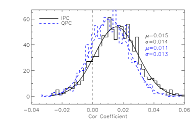
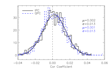
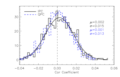
However, it is not truly the time stream correlations that we so much care about, it is the correlations between $Q$ or $U$ for the channels. For instance, if there were a 10% correlation between J1i-$Q$ and J2i-$Q$, it could be hidden in the smaller time stream correlations. We must therefore evaluate these correlations directly.

	$\mathbf{\langle QQ\rangle}$	$\mathbf{\langle UU\rangle}$	$\mathbf{\langle QU\rangle}$	$\mathbf{\langle UQ\rangle}$
$\mathbf{\langle J1\ J2\rangle_{IPC}}$	0.144 $\pm$ 0.034	0.134	-0.024	0.021
$\mathbf{\langle J1\ J2\rangle_{QPC}}$	0.005 $\pm$ 0.034	0.062	-0.011	-0.002
$\mathbf{\langle J1\ J3\rangle_{IPC}}$	0.074 $\pm$ 0.041	0.063	-0.069	-0.003
$\mathbf{\langle J1\ J3\rangle_{QPC}}$	0.023 $\pm$ 0.041	0.048	-0.009	-0.042
$\mathbf{\langle J2\ J3\rangle_{IPC}}$	0.104 $\pm$ 0.041	0.093	-0.024	-0.029
$\mathbf{\langle J2\ J3\rangle_{QPC}}$	0.066 $\pm$ 0.041	0.001	-0.054	-0.047

Table 8.1: ROD Inter-Channel Cross-Correlation Coefficients, calculated from the surviving ROD data. The errors are the same within each row, and assume that the underlying distribution of correlation coefficients is Gaussian.

In order to measure these correlations, we used the ROD data set and found the Pearson’s correlation coefficient in the same way as for the TOD, but because there is so much less data, we found only one correlation coefficient for each surviving section. We then calculated means and errors by averaging from the distribution of these sectional values. Table 8.1 shows these values with their errors. The numbers in this table are very suggestive. For instance, $\langle Q\ Q\rangle$ for all IPC channels is about the same as $\langle U\ U\rangle$, suggesting a common source. All QPC correlation coefficients are consistent with zero, as are all correlations of the $\langle Q\ U\rangle$ variety . Luckily, as $Q$ and $U$ show no correlation between them (either within a channel or between channels), we can keep treating $Q$ and $U$ as completely independent measurements. This is not too surprising, considering they are essentially the $\sin{2\phi}$ and $\cos{2\phi}$ projections from each rotation, which are orthogonal functions. However, the correlations between IPC channels (for the same Stokes parameter) are $\sim$ 10%, so we cannot ignore them in constructing a final map.

Combining non-independent maps : the machinery

Now, how do we add together maps of $Q$ (or $U$) from the three non-independent channels, armed with the knowledge of their mutual correlations? The algorithms in §8.4 did not deal with adding non-independent maps together, but it is relatively easy to expand them. We will treat $Q$ and $U$ separately, as they are completely uncorrelated. Let us consider our situation for $Q$; $U$ will follow an identical format. We have three channel maps, call them ${\bf q}_{1}$, ${\bf q}_{2}$, and ${\bf q}_{3}$, with their corresponding covariance matrices ${\bf\Sigma}_{Q1}$, ${\bf\Sigma}_{Q2}$, and ${\bf\Sigma}_{Q3}$. Let the correlation coefficient between ${\bf q}_{i}$ and ${\bf q}_{j}$ be $\rho_{ij}$. We appeal to Minimum Variance Mapmaking to form the best possible map.

First, we form our “mega-map”, which is the three maps concatenated together, and a corresponding “mega-covariance matrix”:

$${\bf q}_{mega} = \{{\bf q}_{1},{\bf q}_{2},\ {\bf q}_{3}\}$$ (8.33a)

$${\bf\Sigma}_{mega} = \left[\begin{array}[]{ccc}{\bf\Sigma}_{Q1}&\rho_{12}\sqrt{{\bf\Sigma}_{Q1}}\sqrt{{\bf\Sigma}_{Q2}}&\rho_{13}\sqrt{{\bf\Sigma}_{Q1}}\sqrt{{\bf\Sigma}_{Q3}}\\ \rho_{12}\sqrt{{\bf\Sigma}_{Q1}}\sqrt{{\bf\Sigma}_{Q2}}&{\bf\Sigma}_{Q2}&\rho_{23}\sqrt{{\bf\Sigma}_{Q2}}\sqrt{{\bf\Sigma}_{Q3}}\\ \rho_{13}\sqrt{{\bf\Sigma}_{Q1}}\sqrt{{\bf\Sigma}_{Q3}}&\rho_{23}\sqrt{{\bf\Sigma}_{Q2}}\sqrt{{\bf\Sigma}_{Q3}}&{\bf\Sigma}_{Q3}\end{array}\right]$$ (8.33e)

We can take the square roots of the ${\bf\Sigma}$-matrices since they are all positive definite, as long as we add a large offset to each matrix (corresponding to the uncertainty in the offset, which is formally infinite) . The final full covariance matrix, ${\bf\Sigma}_{q}$, will then also have a large offset, but because of the arguments already discussed, this will not affect the final CMB likelihood analysis. We simply must remember that the very large eigenvalue of the final map covariance matrix represents our infinite uncertainty in the overall map offset.

Now that we have re-expressed our individual maps in the “mega-map” and “mega-covariance matrix” format, we apply Minimum Variance Mapmaking. Our pointing matrix is given by

$${\bf A}_{mega}=\left[\begin{array}[]{c}{\bf I}_{n}\\ {\bf I}_{n}\\ {\bf I}_{n}\end{array}\right]\ .$$ (8.34)

This points our three individual maps to the same final map; each ${\bf I}$ is the $n\times n$ identity matrix, where $n$ is the number of pixels in our maps. Explicitly, the final joint map and covariance matrix are given by:

$${\bf q} = {\bf\Sigma}_{q}\ {\bf A}_{mega}^{t}{\bf\Sigma}_{mega}^{-1}{\bf q}_{mega}$$ (8.35a)

$${\bf\Sigma}_{q} = [{\bf A}_{mega}^{t}\ {\bf\Sigma}_{mega}^{-1}{\bf A}_{mega}]^{-1}\quad\text{.}$$ (8.35b)

Because of the large offset each covariance matrix possesses, the final map ${\bf q}$ may have some random offset to it, but it is meaningless, and can be safely subtracted out.

Figure 8.15: Final joint-channel sky maps. The joint IPC maps for $Q$ and $U$ are displayed in (a), while (b) shows the QPC maps.

The final joint-maps for the IPC and QPC are shown in Figure 8.15. Again, we see no evidence of an underlying sky signal. Instead of calculating $\chi^{2}$’s and the like for these maps, in order to determine if they show evidence of a sky signal, the route along which we will proceed is the full Likelihood Analysis in order to constrain a specific model of CMB polarization. This process is described fully in the next chapter.

8.8 A Simple Simulation

The number of steps that the data passed through in the route from time-ordered data to final maps was large, and several of steps were not exactly simple to understand. The chance for errors in at least one of these steps is high, so we found it very useful to generate model data streams for which we knew the underlying signal, and run these “Fake polar Signals” through the full machinery of the data pipeline, to check for errors and make sure that everything worked as anticipated.

8.8.1 Parameters of the Simulation

There were three primary steps involved in the simulation process: build the underlying map, let polar “observe” and generate data based on these “observations”, and then run this data through the full mapmaking analysis, from $TOD\rightarrow Maps$.

Underlying Maps

We built the underlying sky maps out of simple sine and cosine modes. We assumed a basic flat band-power model with $\sim$ 10 $\mu K$ per band, from $\ell\sim 0\ to\ 100$, and then convolved these signals with a 7^∘ Gaussian beam. We assumed the same underlying map for all three channels (thus, only CMB, no foregrounds). We did not need a complicated map because this procedure is not to test foreground removal or parameter extraction, but rather to ensure our map reconstruction algorithms performed well.

Simulated POLAR Observations

To shorten processing time, we made the simulated polar about a factor of two more sensitive than the real polar, with a full sensitivity of $340\mu K\sqrt{sec}$. We included all IPC and QPC channels in the analysis, but no total power channels. We assumed the noise was almost white, with a small amount of 1/f noise in each channel. We convolved each data stream with our 5 Hz anti-aliasing filter. The resulting power spectra from the three IPC channels are shown in Figure 8.16; notice the strong similarity to polar’s true power spectra, such as shown in Figure 4.12.

Figure 8.16: Power spectra of simulated IPC data. Notice the presence of 1/f noise, our 5 Hz anti-aliasing low-pass filter, and also a small peak at the $2\phi$ frequency. The noise-equivalent temperatures for these channels are somewhat better than for actual polar, in order to speed up the processing time (less data were required to reach the same signal level). Otherwise, these power spectra qualitatively match those of polar (when the weather was good) quite well.

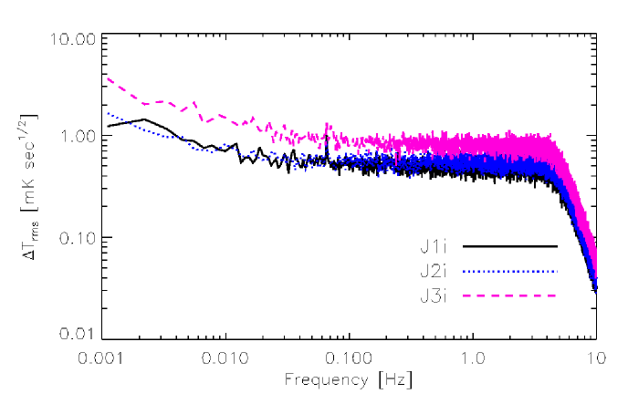
We included the effect of the “AOE” (absolute one-bit encoder), which fired every time polar completed a rotation; the analysis techniques require this data in order to form the ROD data. We even included the short gaps in data taking that occurred after each 7.5 minute data file was written (these gaps were 2-5 seconds long), just in case this might have led to an observable effect in the maps. We also added random offsets in $I_{0}$, $Q$, and $U$ for each section and channel, of levels consistent with those experienced by polar. We generated five sections of data, with a total of 31 hours of observation time. The true polar data set had 49 sections of data, of which about 15 contributed to the final analysis (about 100 hours of data). Additionally, we made the sky signals much larger than theory expects, so the simulation could be run in a reasonable amount of time. The simulation parameters for each channel are shown in Table 8.2.

Channel	NET [$mK\ s^{1/2}$]	1/f Knee	5 Hz Filter	$I_{0}$ [mK]	$Q_{off}$ [$\mu K$]	$U_{off}$ [$\mu K$]
J1i	0.50	0.01	Yes	$3r$	$30r$	$20r$
J2i	0.55	0.005	Yes	$10r$	$60r$	$40r$
J3i	0.80	0.02	Yes	$50r$	$90r$	$60r$
J1o	0.50	0.01	Yes	$0.03r$	$0$	$0$
J2o	0.55	0.005	Yes	$0.1r$	$0$	$0$
J3o	0.80	0.02	Yes	$0.5r$	$0$	$0$

Table 8.2: Simulation parameters for each correlator channel. The “$r$” in several columns indicates a random number between $-1$ and $1$, drawn from a flat distribution. Thus, for example, the $Q$ offsets for channel J1i were between $-20$–$20$ $\mu K$, and were different for each section. Five sections were generated with a total of 31 hours of data.

Simulation Map Reconstruction

We next ran the fake polar signals through the full analysis pipeline, including removing an offset for each section, for all channels, in both $Q$ and $U$ (just as in the real analysis). The derived joint-channel maps are shown in Figure 8.17, along with the underlying sky maps for comparison. The performance of the analysis software was good; the derived maps match the initial maps well, up to an overall offset (and in some cases some other large-scale modes, like a linear term). Recall that we have removed our sensitivity to the largest-scale modes, so these features showing up in our final map will not affect a likelihood analysis. The QPC maps [not shown] were consistent with noise.

Figure 8.17: Derived joint-channel maps for simulated data, for the IPC channels, compared to the underlying sky map. The thin (black) curve is the underlying sky map convolved with a 7^∘ beam. The (blue) data points represent the derived joint-channel IPC map, after the 31 hours of simulated data was run through the entire polar analysis procedure. The fairly high signal-to-noise ratio is due to the excellent noise figures we assumed for the simulated experiment. The signal values are roughly consistent with those of temperature anisotropy levels. The agreement between the underlying maps and those derived from the simulated data is a strong indication of the robustness of our mapmaking algorithms.

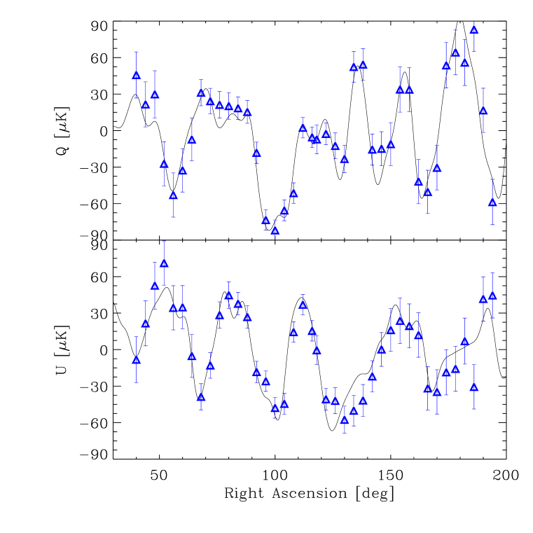
These results lead to a fairly big sigh of relief. It is important to simulate or Monte-Carlo an experiment in order to test the analysis pipeline. Besides being an invaluable debugging tool, it also lends significant credence to the results of the experiment. Even though our experiment produced only upper limits on possible signals, it is still comforting to know that the analysis routines were in principle capable of detecting and mapping signals correctly, had they been present.

Chapter 9 Discussion & Likelihood Analysis

Now that the maps of $Q$ and $U$ have been generated, we seek to answer questions about the level of CMB polarization our data can constrain, either through a detection or new upper limit. Some loftier goals are to constrain the power spectra of polarization fluctuations, the optical depth to reionization, or even the polarization of synchrotron radiation. We shall begin, naturally, with the first, and answer questions about a simple flat band power model CMB polarization.

9.1 Introduction to Bayesian Likelihood Analysis

We employ a Bayesian maximum likelihood analysis in order to characterize the level of possible CMB polarization fluctuations present in our data. As we measured $Q$ and $U$ simultaneously, we are able to set limits on both E- and B-type polarization independently.

The flow of a standard likelihood analysis is as follows. A model is constructed which depends on some set of parameters $\vec{a}=\{a_{1}\ldots a_{m}\}$. We wish to constrain these parameters given the data ${\bf x}$. Unfortunately, all we can calculate is the probability distribution of the data given the parameters, which we denote as $P({\bf x}|\vec{a})$. This is where Bayes’ theorem comes into play, which states that

$$P(\vec{a}|{\bf x})\ \propto\ P({\bf x}|\vec{a})\ P(\vec{a})$$ (9.1)

In words, the probability of the model given the data equals the probability of the data given the model times the prior probability of the model. The probability distribution $P(\vec{a})$ is assumed to be uniform (uninformative). The probability distribution $P({\bf x}|\vec{a})$ is given by the likelihood function,

$${\bf\mathcal{L}}(\vec{a})\ =\ \frac{1}{{2\pi}^{N/2}}\frac{e^{-\frac{1}{2}{\bf x}^{t}{\bf C}(\vec{a}){\bf x}}}{|{\bf C}|^{1/2}}$$ (9.2)

where N is the number of pixels in the map ${\bf x}$, and ${\bf C}(\vec{a})$ is the full covariance matrix, given by the sum of data and theory covariance matrices:

$${\bf C}\ =\ {\bf S}\ +{\bf\Sigma}\quad.$$ (9.3)

Note that ${\bf C}$ and ${\bf S}$ both inherently depend upon the parameters $\vec{a}$. The likelihood function is simply denoted ${\bf\mathcal{L}}(\vec{a})$, rather than say ${\bf\mathcal{L}}({\bf x}|\vec{a})$, because our data is not changeable at this point, only the model is, so any reference to the data varying has been dropped. In all cases, the data vector is given by ${\bf x}\equiv\{{\bf q},\ {\bf u}\}$, where ${\bf q}$ and ${\bf u}$ are the $Q$ and $U$ joint-channel maps, respectively, as constructed in §8.7.4. Each contains $N=84$ pixels of 2^∘ width in right ascension on the sky at $\delta=43^{\circ}$. The data covariance matrix ${\bf\Sigma}$ is formed from the covariance matrices for the joint-channel maps as calculated in §8.7.4 such that

$${\bf\Sigma}\ =\ \left[\begin{array}[]{cc}{\bf\Sigma}_{Q}&0\\ 0&{\bf\Sigma}_{U}\end{array}\right]\quad.$$ (9.6)

At this point we find the maximum of the likelihood function in the parameter space $\vec{a}$, denoted $\vec{a}_{M}$; this point determines the maximally likely set of $\vec{a}$. In order to determine the error bars on these parameters, we find the Bayesian credible region in parameter space about $\vec{a}_{M}$, a region of volume $V$ bounded by a surface of constant ${\bf\mathcal{L}}$ such that

$$\int_{V}{\bf\mathcal{L}}(\vec{a})d\vec{a}\ =\ c\int{\bf\mathcal{L}}(\vec{a})d\vec{a}\quad,$$ (9.7)

where the integral on the right is an integral over all of $\vec{a}$-space, and $c$ is the one minus the desired level of confidence for the region $V$. Then we say that the true set of parameters $\vec{a}_{true}$ lives somewhere in the region $V$ with a level of confidence $c$.

9.2 Limits on E and B in a Flat Band-Power Model

We will set limits on the E- and B-type polarizations of the CMB by assuming a flat band-power model. This model has only two free parameters, $T_{E}$ and $T_{B}$, and the power spectra are given by

$$\ell(\ell+1)C_{\ell}^{X}/2\pi=T^{2}_{X}$$ (9.8)

where $X\in\{E,B\}$. $T_{E}$ and $T_{B}$ then correspond to the RMS-level of fluctuations in E- and B-mode polarization, respectively.

9.2.1 Constructing the Theory Covariance Matrix

The construction of ${\bf S}$ is fairly involved; its derivation is introduced in [145], and given in great detail in [144]. ${\bf S}$ is a $2N\times 2N$ matrix, which we will consider as an $N\times N$ matrix whose elements are $2\times 2$ matrices. The $2\times 2$ elemental matrix ${\bf S}_{ij}$ describes the covariance between two pixels $i$ and $j$, and is given by

$${\bf S}_{ij}\ =\ \langle{\bf x}_{i}{\bf x}_{j}\rangle={\bf R}(\alpha_{ij}){\bf M}(\hat{{\bf r_{i}}}\cdot\hat{{\bf r_{j}}}){\bf R}(\alpha_{ij})^{t}$$ (9.9)

where $\hat{{\bf r_{i}}}$ and $\hat{{\bf r_{j}}}$ are the unit vectors pointing to pixels $i$ and $j$, respectively. ${\bf R}(\alpha_{ij})$ is a standard rotation matrix which rotates the $(Q,U)$ components in ${\bf M}$ into the global coordinate system where the reference frame for $Q$ and $U$ is given by the local meridian ; it is given by

$${\bf R}({\bf\alpha})\ =\ \left(\begin{array}[]{cc}\cos{2\alpha}&\sin{2\alpha}\\ -\sin{2\alpha}&\cos{2\alpha}\end{array}\right)$$ (9.12)

The covariance matrix ${\bf M}$ depends only on the angular separation between the pixels $i$ and $j$. ${\bf M}$ is most naturally expressed in a coordinate system such that the great circle connecting pixels $i$ and $j$ serves as the reference axis for the Stokes parameters [49]. Expressed in this coordinate frame, ${\bf M}$ becomes [145]

$${\bf M}(\hat{{\bf r_{i}}}\cdot\hat{{\bf r_{j}}})\equiv\left(\begin{array}[]{cc}\langle Q_{i}Q_{j}\rangle&0\\ 0&\langle U_{i}U_{j}\rangle\end{array}\right)\quad,$$ (9.15)

$$\langle Q_{i}Q_{j}\rangle \equiv \sum_{\ell}\left(\frac{2\ell+1}{4\pi}\right)B_{\ell}^{2}\ [F^{12}_{\ell}(z)C_{\ell}^{E}-F^{22}_{\ell}(z)C_{\ell}^{B}]$$ (9.16a)

$$\langle U_{i}U_{j}\rangle \equiv \sum_{\ell}\left(\frac{2\ell+1}{4\pi}\right)B_{\ell}^{2}\ [F^{12}_{\ell}(z)C_{\ell}^{B}-F^{22}_{\ell}(z)C_{\ell}^{E}]\quad$$ (9.16b)

where $z=\hat{{\bf r_{i}}}\cdot\hat{{\bf r_{j}}}$ is the cosine of the angle between the two pixels under consideration, $B_{\ell}=\exp[-\ell(\ell+1)\sigma^{2}_{B}/2]$, $\sigma_{B}$ is the beam dispersion $=0.425\times\,$FWHM, and $F^{12}_{\ell}$,$F^{22}_{\ell}$ are functions of Legendre polynomials as defined in [145, 144]. The full matrix ${\bf S}$ is then constructed by looping over all necessary pixel pairs. In principle, ${\bf S}$ needs to be calculated for all ($T_{E}$,$T_{B}$) combinations in order to fully assess the likelihood function. However, there is a great simplification lurking here. Recalling that for the flat band-power model, $\ell(\ell+1)C_{\ell}^{X}/2\pi=T^{2}_{X}$ with $X\in\{E,B\}$, Equation (9.9) can be recast as

$${\bf S}_{ij}\ =\ T_{E}^{2}\ {\bf S}_{ij}^{E}\ +\ T_{B}^{2}\ {\bf S}_{ij}^{B}\quad,$$ (9.17)

$${\bf S}_{ij}^{X}\ \equiv\ {\bf R}(\alpha_{ij})\sum_{\ell}\frac{2\ell+1}{2\pi\ell(\ell+1)}B_{\ell}^{2}\mathbf{F_{\ell}}^{X}(z){\bf R}(\alpha_{ij})^{t}\cdot(1\ \mu K^{2})$$ (9.18)

where

$$\mathbf{F_{\ell}}^{E}(z)\equiv\left[\begin{array}[]{cc}F^{12}_{\ell}(z)&0\\ 0&-F^{22}_{\ell}(z)\end{array}\right]\quad\text{and}\quad\mathbf{F_{\ell}}^{B}(z)\equiv\left[\begin{array}[]{cc}-F^{22}_{\ell}(z)&0\\ 0&F^{12}_{\ell}(z)\end{array}\right]$$ (9.19)

The theory covariance matrix ${\bf S}$ in the flat band-power model is then given by

$${\bf S}(T_{E},T_{B})\ =\ T_{E}^{2}\ {\bf S}^{E}\ +T_{B}^{2}\ {\bf S}^{B}$$ (9.20)

where ${\bf S}^{E}$ is the fundamental theory covariance matrix for purely E-modes, comprised of all the 2$\times$2 ${\bf S}^{E}_{ij}$ matrices, and similarly for ${\bf S}^{B}$. Now we must must merely calculate ${\bf S}^{E}$ and ${\bf S}^{B}$ once each, and we can then evaluate the full theory covariance matrix for any ($T_{E}$,$T_{B}$) pair we like using Equation (9.20).

Figure 9.1: Gaussian beam function $B_{\ell}$ for polar’s 7^∘ FWHM beam. Our main sensitivity in $\ell$-space decreases rapidly after $\ell\sim 20$. Originally calculated in [102].

Figure 9.2: Plots of the ra = 40^∘ row of the fundamental signal covariance matrices ${\bf S}^{E}$ and ${\bf S}^{B}$. The four panels in the plot correspond to the four quadrants of the matrices as labelled. The thick solid line represents ${\bf S}^{E}$, the thick dashed line represents ${\bf S}^{B}$, and the thin solid line corresponds to a 7^∘ Gaussian beam for reference.

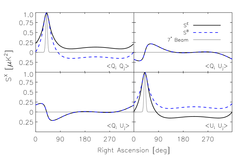
The signal covariance matrices were calculated for our 2^∘ pixelization spanning all 360^∘ of right ascension, using as an approximation to our beam a single 7^∘ FWHM Gaussian, in order to calculate our beam function $B_{\ell}$ for use in Equations (9.16). This beam function is essentially our window function for the flat band-power model, and is shown in Figure 9.1. A representative row from both fundamental signal covariance matrices, ${\bf S}^{E}$ and ${\bf S}^{B}$, is shown in Figure 9.2 . This shows the covariance between the pixel at right ascension 40^∘ and all the other pixels. Notice how wide the main peak in the distribution is; the width of this peak ($\sim$ 20^∘) corresponds roughly to the mean $\ell$-value we are probing with this model, which is around an $\ell$ of 10. Our 7^∘ beam is shown for comparison. Also witness the symmetry between E and B; the $\langle U_{i}U_{j}\rangle$ portion of ${\bf S}^{E}$ is the same as the $\langle Q_{i}Q_{j}\rangle$ portion of $Sc^{B}$, and vice-versa. All of the $\langle Q_{i}U_{j}\rangle$ pieces are identical. This shows the general behavior of the matrix, as all other rows are identical to this row, except shifted such that the peak lies over the pixel in question.

9.2.2 Evaluating the Likelihood Function

Now that we have constructed the theory covariance matrix for our parameter space of ($T_{E},T_{B}$), we are in a position to calculate the likelihood of our data given this set of models, as defined in Equation (9.2).

There are two basic calculations that we must perform in order to evaluate the likelihood ${\bf\mathcal{L}}$ for any set of ($T_{E},T_{B}$): the exponent factor ${\bf x}^{t}{\bf C}{\bf x}$, and the square root of the determinant of ${\bf C}$. Appendix 9.6 describes how to do this was performed, using the Cholesky decomposition.

Figure 9.3 shows the likelihood function as evaluated for all individual and joint channel maps, both for the IPC and QPC (null channels). It is consistent with upper limits in all cases. The values in the upper corner are the values of the likelihood where they cross $T_{E}=T_{B}=0$. These yield 95% confidence limits of 10.0 $\mu K$ on both $T_{E}$ and $T_{B}$. As the B-polarization at large angular scales is assumed to be so much weaker than E-polarization, we can can set $T_{B}$ to be zero; the resulting likelihood function for $T_{E}$ is shown in Figure 9.4. It yields a 95% confidence limit of $T_{E}<\ 7.7\mu K$.

Figure 9.3: Normalized likelihood contour plots in the $T_{E}-T_{B}$ plane. The contours enclose are $68\%$, $95.4\%$, and $99.7\%$ of the total probability, corresponding to $1,2,$ and $3$ standard deviation intervals, as labelled. The solid lines correspond to the likelihood for the IPC frequency channels, and the dashed lines are the corresponding null-channel (QPC) likelihood. The numbers in the upper right corners are ${\bf\mathcal{L}}(0)$, the upper (lower) number corresponds to the IPC (QPC) channel. All likelihoods are consistent with non-detections.

Figure 9.4: Normalized likelihood plot of $T_{E}$, with the prior constraint that $T_{B}=0$. The solid line is the result for the in-phase channels, and the dashed line is for the quad-phase (null) channels. The resulting upper limit is $T_{E}<\ 7.7\mu K$ at 95% confidence.

9.2.3 The Co-added Channel Analysis

It is worth noting that the entire mapmaking analysis in Chapter 8 can be redone in a slightly different way, where the three channels are combined in the Time-Ordered Data. This technique automatically takes into account any correlations that may be present between the channels. One simply co-adds the timestreams with their inverse noise weightings in order to obtain a time stream with the maximum possible signal. Offset removal is still done on the submaps, but since we have combined the channels, a single offset is removed for $Q$ and $U$ for a two of two offsets per section removed (rather than six for the individual-channel analysis).

This was performed for our data, and the corresponding likelihood contours were calculated. The upper limits remain, but have been degraded to about 12 $\mu K$. This makes sense, considering we subtracted only two offsets per section, not six as in the primary analysis. Because the offsets were not perfectly correlated among the three channels, there was residual power left over in the maps due to the imperfect co-addition of the channel offsets; it was this phenomenon that led to the slightly worse upper limits. This result notwithstanding, this analysis is important in that it shows our inter-channel correlations were not a strong problem.

9.3 Power Spectra

It is possible to use the same formalism as in §9.2 to estimate band-powers for the individual $C_{\ell}^{EE}$ and $C_{\ell}^{BB}$ polarization power spectra. In this case, a separate theory covariance matrix is constructed for each band-power to be estimated, and errors are determined from the corresponding likelihood functions, exactly as in the previous case. Our collaborators applied these techniques, and generated window functions to estimate each band power. However, there is a new twist on band-powers when it comes to polarization; there is some leakage of E-power into the B-mode estimation, and vice-versa, and this depends on how one chooses to construct the window functions. Tegmark and de Oliveira-Costa show how to minimize this leakage in [144].

The window functions were generated with these minimum leakage techniques; the results are shown in Figure 9.5. The leakage of $B$ into $E$ is exactly symmetric for $E$ into $B$, thus we show only the $E$ window functions. The leakage factor is appreciable, as we can see from the figures. This is primarily a consequence of polar’s limited scan region and one-dimensional geometry. Due to this non-negligible leakage, we should treat the resulting power spectra with reasonable caution.

(a) $\ell=7$ $E$ Window Function

(b) $\ell=15$ $E$ Window Function

Figure 9.5: The window functions for $E$ used to estimate the band powers. These functions effectively show our sensitivity to $E$ or $B$ for any $\ell$-value, when we are aiming for a certain multipole. The $B$ window functions are exactly the same as for $E$ (with $E$ and $B$ switched, of course). There is significant leakage of $B$-power into the $E$-estimate because of the scan strategy. In general, more circular scan strategies with larger sky coverage will have a much better $E$-$B$ separation, and narrower window functions. The width of the window function scales with the inverse of the sky patch size in its narrowest dimension [144]. Figure by Angelica de Oliveira-Costa.

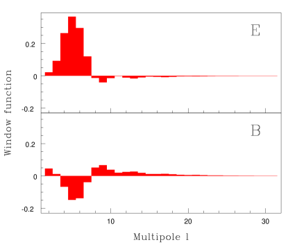
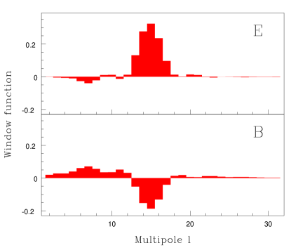
Given this precaution, we constructed band-power estimates from our final joint channel data, for both $E$ and $B$; these estimates are again consistent with upper limits and are shown in Figure 9.6. Some of the estimates are negative. This is because the models use a free parameter which is roughly $power^{2}$, and the likelihood function does not know that this parameter is not allowed to go negative, therefore sometimes the best estimate comes out to be a little less than zero. This is, of course, consistent with a non-detection and is nothing to worry about.

These upper limits are still significantly higher than any possible reionization peak (which must be less than about 2 $\mu K$, even for an optical depth to reionization of $1.0$ [57, 58]); therefore, this data set cannot say anything interesting about reionization. We still emphasize that it is very instructive simply going through the process of forming the band-powers; this can help possibly design future experiments. For instance, it is virtually impossible to make band-power estimates without observations of both $Q$ and $U$ on the same part of the sky. I am not aware of any current methods to limit polarization power spectra without simultaneous knowledge of both $Q$ and $U$.

Figure 9.6: Band Power Estimates for $E$ and $B$, from the combined channel IPC data. We show the data point at $\ell=30$ to illustrate how fast the window function cuts off; after about $\ell=20$, almost all useful information has been extracted from the power spectra. Figure by Angelica de Oliveira-Costa.

9.4 A Word About Foregrounds

As our results are all inconsistent with a detection of any type, foregrounds were not a problem for this experiment at the level of sensitivity we reached. As we discussed in Chapter 2, synchrotron is most probably the strongest polarized foreground at our frequencies. However, both the spectral index and the polarization fraction of synchrotron are not well known, and in fact vary from place to place on the sky.

In order to model the expected synchrotron signal as seen by polar, we extrapolated the Haslam 408 MHz radio map (which is dominated by synchrotron) to our frequencies via several models. Figure 9.7 shows four models, representing 10% and 50% fractional polarization, as well as a synchrotron spectral index from 5 to 31 GHz of -2.8 and -3.1. We use these merely as representative examples. In all cases we assumed a spectral index of -2.8 from 408 MHz to 5 GHz, where there are good measurements (e.g. , see [70]). The figure also shows the polar data set for total polarization (that is, $\sqrt{Q^{2}+U^{2}}$), along with approximate error bars. We see that the 50% polarization data for both choices of spectral index is inconsistent with the data (although the steeper spectral index is only marginally inconsistent), which favors roughly 0–20% polarization. A more rigorous analysis planned for the near future will be able to simultaneously constrain the spectral index and large angular scale polarization of synchrotron, using formalism outlined in [90] and [66].

Figure 9.7: Comparison of polar maps with various synchrotron models. All models employed the Haslam 408 MHz data, extrapolated to 5 GHz using a synchrotron spectral index of $\alpha=-2.8$, and smoothed with a 7^∘ beam. Extrapolation from 5 to 31 GHz used an index of $\beta=-2.8$ (thin lines) and $\beta=-3.1$ (thick lines). Polarization fractions assumed are 10% (solid lines) and 50% (dashed lines). It is clearly possible to set limits on polarized synchrotron with the polar data, which is planned for a near-future analysis.

Had we seen a signal, the situation would be much more confusing, because we would have been faced with the difficult task of determining whether our signal was due to CMB or foregrounds. However, the task is not quite as daunting as it seems. One simple test is to assess how strong the $E$-signal is as compared to the $B$-signal; if they are of comparable magnitudes, then most likely foregrounds are dominating the signal, but if $B$ is consistent with zero and E is consistent with signal, this is strong evidence of a CMB-dominated signal. Doubtless this will be among the first tests employed by groups to assess foreground contamination, and it is a test that is not possible in corresponding anisotropy experiments.

9.5 Final Thoughts

The polar experiment was first envisioned in the early 1990s, built in the late 1990s, deployed and operated in the year 2000, and the initial analysis was completed in 2001. By the time it ran, the project employed fairly old technology and was deployed at a highly non-optimal site, yet still was able to set the most stringent limits to date on CMB polarization. This speaks highly of the potential to do MUCH better in the measurement of CMB polarization. By moving our experiment to say, White Mountain or the Atacama desert, it is not unreasonable to expect 3 months of good observations in a year; considering the site elevations and using state of the art HEMTs, a system temperature of 20 K is very attainable in $K_{a}$ band. If the offset issue could be eliminated, this naively would lead to limits closer to 0.5 $\mu K$, a factor of twenty better than the limits quoted in this thesis, and those limits are still for a simple one-receiver system. Clearly, the field is wide-open for significantly better limits on, or a measurement of, CMB polarization.

It is well-known that the best chance of detecting polarization is in the temperature-polarization cross-correlations. Although polar likely did not see this effect (it is theorized to be $\lesssim 1$ $\mu K$ for $\ell<20$ in even the most optimistic scenarios), time permitting we plan to carry out the cross-correlation analysis, simply because no one ever has before, and we can possibly place more stringent limits on the polarization. The COBE data is well-suited for this correlation, considering its full-sky coverage and 7^∘ beam size. Undoubtedly much can be learned by simply performing the analysis on real-world data.

After polar was “de-commissioned” in the summer of 2000, it was coupled with a 2.6 meter primary dish; this experiment is known as compass COsmic Microwave Polarization At Small Scales. Given that compass is using the receiver from polar, and that the polarization signals at $\ell\sim 600$ is about a factor of one hundred higher (they are on the order of 2-5 $\mu K$) than for large scales, compass has a good chance of detecting the polarization. Future plans call for upgrading the polar-compass projects to have several pixels at both $Q$ and $W$ bands, which will really help open up this new and exciting field.

9.6 Likelihood Function Evaluation using Cholesky Decomposition

For a data set ${\bf x}$ and total covariance matrix ${\bf C}$, the likelihood of the data given the model is given by

$${\bf\mathcal{L}}\ =\ \frac{1}{{2\pi}^{N/2}}\frac{e^{-\frac{1}{2}{\bf x}^{t}{\bf C}^{-1}{\bf x}}}{|{\bf C}|^{1/2}}$$ (9.21)

This can be troublesome to evaluate if ${\bf C}$ is large or ill-conditioned, especially if a straightforward inversion of ${\bf C}$ is attempted. A better way to go about this is to use Cholesky decomposition as described by Barth Netterfield in his thesis [146]. The matrix ${\bf C}$ is symmetric and positive definite; therefore there exists a non-trivial Cholesky factorization of such that ${\bf C}$ = ${\bf L}{\bf L}^{t}$, where ${\bf L}$ is a lower-triangular matrix.

Often what is actually evaluated is the natural log of the likelihood, such that

$$\ln{{\bf\mathcal{L}}}=-1/2\chi^{2}\ -\ \ln{|{\bf C}|^{1/2}}+const\quad,$$ (9.22)

where $\chi^{2}\equiv{\bf x}^{t}{\bf C}^{-1}{\bf x}$. As we only care about the relative shape and peak position of the likelihood, the overall constant is immaterial.

Due to the Cholesky factorization, the middle term in Equation (A2) is simply

$$\ln{|{\bf C}|^{1/2}}=\ln{|{\bf L}|}=\sum_{i}\ln{\lambda_{i}}\ ,$$ (9.23)

where the $\lambda_{i}$ are the values on the diagonal of ${\bf L}$, and incidentally are also the square roots of the eigenvalues of ${\bf C}$. Evaluating the $\chi^{2}$ piece of Equation (A2) is also relatively easy. We note that

$$\chi^{2} = {\bf x}^{t}{\bf C}^{-1}{\bf x}={\bf x}^{t}({\bf L}{\bf L}^{t})^{-1}{\bf x}$$

$$= {\bf x}^{t}({\bf L}^{t})^{-1}{\bf L}^{-1}{\bf x}=({\bf L}^{-1}{\bf x})^{t}{\bf L}^{-1}{\bf x}$$

$$= {\bf y}^{t}{\bf y}$$

where I have defined ${\bf y}\equiv{\bf L}^{-1}{\bf x}$. We then simply solve for ${\bf y}$ by finding ${\bf y}$ in ${\bf L}{\bf y}={\bf x}$, which is easily done considering ${\bf L}$ is triangular.

Overall, this technique is far superior to directly evaluating the inverse of ${\bf C}$, because it is both faster and far less subject to round-off error. In fact, there are standard Numerical Recipes procedures choldc and cholsol that make the procedure relatively simple. The routine choldc can be used to find ${\bf L}$ and hence the determinant factor in Equation (A2). The routine cholsol solves ${\bf C}{\bf\eta}={\bf x}$ for the vector $\mathbf{\eta}={\bf C}^{-1}{\bf x}$, so we have simply $\chi^{2}={\bf x}^{t}\mathbf{\eta}$.

Appendix A POLAR Glossary of Terms

$\mathbf{1\phi}$

Term used to reference the fundamental rotational frequency of polar, or physical processes occurring at that frequency; this frequency is $\sim$ 0.0325 Hz, corresponding to a period of about 30.6 sec per rotation.

$\mathbf{2\phi}$

Term used to describe twice the rotation frequency of polar, or physical processes occurring at that frequency; this frequency is $\sim$ 0.065 Hz.

AOE

Absolute One-Bit Encoder. This little wonder was mounted to the rotating stage of polar, and fired a TTL pulse whenever polar passed through a certain rotation angle. This was our central means of determining what rotation angle polar was at for any given time.

DSC

Dielectric Sheet Calibrator, the calibrator system polar used, described in Chapter 5.

HEMT

High-Electron Mobility Transistor, amplifiers which when cooled have very low noise. These served as our first stage of gain, and set the primary noise of the system.

HF (Hour File)

One data file, 7.5 minutes in length. Each HF contained exactly 9000 samples per channel (of which there were 16, see Table 4.3).

IPC

In-Phase Channels. The polar instrument had a phase chopper that chopped the LO signal between 0^∘ and 180^∘ at 967 Hz. The final correlator signals from each of our three frequency sub-bands were then locked into with a lock-in amplifier, using both the actual chop reference signal, and a signal 90^∘ out of phase with that. The IPC represent the signals from the lock-in amplifier obtained using the in-phase chopper reference.

Noise Equivalent Temperature (NET)

The signal level an experiment can detect at 1$\sigma$ in one second of integration time, with units of $K\sqrt{sec}$.

POLAR

Polarization Observations of Large Angular Regions, the experiment this thesis describes.

Pointing Matrix

General term for a matrix that produces a data stream when it operates on the underlying map. Throughout this thesis, it is always referred to as ${\bf A}$ (or some variant). The pointing matrix is determined entirely by the scan strategy; if there are $N_{pix}$ pixels in the underlying map, and $N_{samples}$ in the data vector, then the pointing matrix will be a $N_{samples}\times N_{pix}$ rectangular matrix.

QPC

Same as using the quad-phase chopper reference signal. In principle, this channel should only be sensitive to the receiver noise, but not sensitive to any signals.

Radbox

Our name for the warm radiometer box which housed the warm RF and IF microwave components of the system.

ROD

Rotation-Ordered Data. A timestream of the rotational coefficients, one for each pixel per Hour File. Thus, a given HF typically has 1-2 sets of rotational coefficients, depending on how many sky pixels it viewed.

Rotational Coefficients

A set of coefficients for the first few terms in the Fourier series expansion of a data segment, with respect to the fundamental rotation frequency of polar, $f_{0}\simeq 0.0325$ Hz. These coefficients we call $c$,$s$,$q$, and $u$, which correspond to the expansion terms $\sin{(2\pi f_{0}t)}$, $\cos{(2\pi f_{0}t)}$, $\sin{(4\pi f_{0}t)}$, and $\cos{(4\pi f_{0}t)}$, respectively.

Rotation

One rotation of the instrument, which takes about 30.6 seconds.

Section

Any of 49 contiguous periods of data when the dome was open and data was being taken, with no calibrations occurring during this period. This term is sometimes also used to describe one such period, after the data cuts have been applied, depending on the context.

Submap

A map and covariance matrix of the sky, for some specific channel, corresponding to the data within a given section that survive all the cuts. Submaps typically contain 6–30 sky pixels, each 2^∘ wide in Right Ascension.

TOD

Time-Ordered Data. The raw data stream whenever we were viewing the sky (and not calibrating).

Total Powers

The two channels of polar that were only sensitive to the intensity of in-band microwaves incident upon our system. These two channels were named TP0 and TP1, and corresponded to the two orthogonal polarizations incident upon the radiometer. They were not included in the signal analysis because 1/f noise from the HEMTs dominated their noise figures, making them $\sim$ 10 times less sensitive than the correlator channels.

References

- [1] S. Perlmutter, G. Aldering, G. Goldhaber, R. A. Knop, P. Nugent, P. G. Castro, S. Deustua, S. Fabbro, A. Goobar, D. E. Groom, I. M. Hook, A. G. Kim, M. Y. Kim, J. C. Lee, N. J. Nunes, R. Pain, C. R. Pennypacker, R. Quimby, C. Lidman, R. S. Ellis, M. Irwin, R. G. McMahon, P. Ruiz-Lapuente, N. Walton, B. Schaefer, B. J. Boyle, A. V. Filippenko, T. Matheson, A. S. Fruchter, N. Panagia, H. J. M. Newberg, W. J. Couch, and The Supernova Cosmology Project, “Measurements of Omega and Lambda from 42 High-Redshift Supernovae,” ApJ, vol. 517, pp. 565–586, June 1999.
- [2] A. G. Riess, A. V. Filippenko, P. Challis, A. Clocchiatti, A. Diercks, P. M. Garnavich, R. L. Gilliland, C. J. Hogan, S. Jha, R. P. Kirshner, B. Leibundgut, M. M. Phillips, D. Reiss, B. P. Schmidt, R. A. Schommer, R. C. Smith, J. Spyromilio, C. Stubbs, N. B. Suntzeff, and J. Tonry, “Observational Evidence from Supernovae for an Accelerating Universe and a Cosmological Constant,” AJ, vol. 116, pp. 1009–1038, Sept. 1998.
- [3] A. V. Filippenko and A. G. Riess, “Results from the high-z supernova search team,” Physics Reports, vol. 307, pp. 31–44, 1998.
- [4] D. Tytler, J. M. O’Meara, N. Suzuki, and D. Lubin, “Review of Big Bang nucleosynthesis and primordial abundances,” Physica Scripta Volume T, vol. 85, pp. 12–31, 2000.
- [5] S. Burles, K. M. Nollett, and M. S. Turner, “Big Bang Nucleosynthesis Predictions for Precision Cosmology,” ApJ, vol. 552, pp. L1–L5, May 2001.
- [6] A. A. Penzias and R. W. Wilson, “A measurement of excess antenna temperature at 4080 Mc/s,” ApJ, vol. 142, pp. 419, 1965.
- [7] G. Gamow, “The origin of elements and the separation of galaxies,” Physical Review, vol. 74, pp. 505, 1948.
- [8] R. H. Dicke, P. J. E. Peebles, P. G. Roll, and D. T. Wilkinson, “Cosmic Black-Body Radiation,” ApJ, vol. 142, pp. 414–419, July 1965.
- [9] P. J. E Peebles, Principles of Physical Cosmology, Princeton Univ. Press, Princeton, NJ, 1993.
- [10] J. C. Mather, D. J. Fixsen, R. A. Shafer, C. Mosier, and D. T. Wilkinson, “Calibrator Design for the COBE Far-Infrared Absolute Spectrophotometer (FIRAS),” ApJ, vol. 512, pp. 511–520, Feb. 1999.
- [11] J. C. Mather, E. S. Cheng, D. A. Cottingham, R. E. Eplee, D. J. Fixsen, T. Hewagama, R. B. Isaacman, K. A. Jensen, S. S. Meyer, P. D. Noerdlinger, S. M. Read, L. P. Rosen, R. A. Shafer, E. L. Wright, C. L. Bennett, N. W. Boggess, M. G. Hauser, T. Kelsall, S. H. Moseley, R. F. Silverberg, G. F. Smoot, R. Weiss, and D. T. Wilkinson, “Measurement of the cosmic microwave background spectrum by the COBE FIRAS instrument,” ApJ, vol. 420, pp. 439–444, Jan. 1994.
- [12] George Smoot and Douglas Scott, “The Cosmic Background Radiation,” 1996, astro-ph/9711069.
- [13] D. J. Fixsen, E. S. Cheng, J. M. Gales, J. C. Mather, R. A. Shafer, and E. L. Wright, “The Cosmic Microwave Background Spectrum from the Full COBE FIRAS Data Set,” ApJ, vol. 473, pp. 576+, Dec. 1996.
- [14] DIMES Mission Home Page, http://map.gsfc.nasa.gov/DIMES/.
- [15] R. K. Sachs and A. M. Wolfe, “Perturbations of a Cosmological Model and Angular Variations of the Microwave Background,” ApJ, vol. 147, pp. 73+, Jan. 1967.
- [16] W. Hu, N. Sugiyama, and J. Silk, “The Physics of Microwave Background Anisotropies,” Nature, vol. 386, pp. 37–43, 1996, virtual tour at http://background.uchicago.edu/.
- [17] D. I. Novikov and H. E. Jorgensen, “A Theoretical Investigation of the Topology of the Cosmic Microwave Background Anisotropy on the Scale 1 degree,” ApJ, vol. 471, pp. 521+, Nov. 1996.
- [18] S. Church, A. Jaffe, and L. Knox, “CMB and Inflation: the report from Snowmass 2001,” Nov. 2001, astro-ph/0111203.
- [19] C. B. Netterfield, P. A. R. Ade, J. J. Bock, J. R. Bond, J. Borrill, A. Boscaleri, K. Coble, C. R. Contaldi, B. P. Crill, P. de Bernardis, P. Farese, K. Ganga, M. Giacometti, E. Hivon, V. V. Hristov, A. Iacoangeli, A. H. Jaffe, W. C. Jones, A. E. Lange, L. Martinis, S. Masi, P. Mason, P. D. Mauskopf, A. Melchiorri, T. Montroy, E. Pascale, F. Piacentini, D. Pogosyan, F. Pongetti, S. Prunet, G. Romeo, J. E. Ruhl, and F. Scaramuzzi, “Multiple Peaks in the Angular Power Spectrum of the Cosmic Microwave Background: Significance and Consequences for Cosmology,” submitted to ApJ, May 2001.
- [20] N. W. Halverson, E. M. Leitch, C. Pryke, J. Kovac, J. E. Carlstrom, W. L. Holzapfel, M. Dragovan, J. K. Cartwright, B. S. Mason, S. Padin, T. J. Pearson, M. C. Shepherd, and A. C. S. Readhead, “DASI First Results: A Measurement of the Cosmic Microwave Background Angular Power Spectrum,” submitted to ApJ, 2001, astro-ph/0104489.
- [21] A. T. Lee, P. Ade, A. Balbi, J. Bock, J. Borrill, A. Boscaleri, P. de Bernardis, P. G. Ferreira, S. Hanany, V. V. Hristov, A. H. Jaffe, P. D. Mauskopf, C. B. Netterfield, E. Pascale, B. Rabii, P. L. Richards, G. F. Smoot, R. Stompor, C. D. Winant, and J. H. P. Wu, “A High Spatial Resolution Analysis of the MAXIMA-1 Cosmic Microwave Background Anisotropy Data,” ApJ, vol. 561, pp. L1–L5, Nov. 2001.
- [22] Lawrence Krauss, “Space, Time, and Matter: Cosmological Parameters 2001,” 2001, astro-ph/0102305.
- [23] X. Wang, M. Tegmark, and M. Zaldarriaga, “Is cosmology consistent?,” May 2001, submitted to Phys. Rev. D, astro-ph/0105091.
- [24] M. Tegmark and et al., “Latest Cosmological Constraints on the Densities of Hot and Cold Dark Matter,” 2001, astro-ph/0008145.
- [25] W. Saunders, W. J. Sutherland, S. J. Maddox, O. Keeble, S. J. Oliver, M. Rowan-Robinson, R. G. McMahon, G. P. Efstathiou, H. Tadros, S. D. M. White, C. S. Frenk, A. Carraminana, and M. R. S. Hawkins, “PSCz catalog (Saunders+, 2000),” VizieR On-line Data Catalog: VII/221. Originally published in: 2000MNRAS.317…55S, vol. 7221, pp. 0+, May 2000.
- [26] W. L. Freedman, B. F. Madore, B. K. Gibson, L. Ferrarese, D. D. Kelson, S. Sakai, J. R. Mould, R. C. Kennicutt, H. C. Ford, J. A. Graham, J. P. Huchra, S. M. G. Hughes, G. D. Illingworth, L. M. Macri, and P. B. Stetson, “Final Results from the Hubble Space Telescope Key Project to Measure the Hubble Constant,” ApJ, vol. 553, pp. 47–72, May 2001.
- [27] J. E. Gunn and B. A. Peterson, “On the Density of Neutral Hydrogen in Intergalactic Space,” ApJ, vol. 142, pp. 1633–1636, Nov. 1965.
- [28] P. M. Lubin and G. F. Smoot, “Search for linear polarization of the cosmic background radiation,” Physical Review Letters, vol. 42, pp. 129–132, Jan. 1979.
- [29] N. Caderni, R. Fabbri, B. Melchiorri, F. Melchiorri, and V. Natale, “Polarization of the microwave background radiation. I - Anisotropic cosmological expansion and evolution of the polarization states. II - an infrared survey of the sky,” Phys. Rev. D, vol. 17, pp. 1901–1918, Apr. 1978.
- [30] Jr. Nanos, G. P., “Polarization of the blackbody radiation at 3.2 centimeters,” ApJ, vol. 232, pp. 341–347, Sept. 1979.
- [31] P. M. Lubin and G. F. Smoot, “Polarization of the cosmic background radiation,” ApJ, vol. 245, pp. 1–17, Apr. 1981.
- [32] P. Lubin, P. Melese, and G. Smoot, “Linear and circular polarization of the cosmic background radiation,” ApJ, vol. 273, pp. L51–L54, Oct. 1983.
- [33] R. B. Partridge, J. Nowakowski, and H. M. Martin, “Linear polarized fluctuations in the cosmic microwave background,” Nature, vol. 331, pp. 146+, Jan. 1988.
- [34] E. B. Fomalont, R. B. Partridge, J. D. Lowenthal, and R. A. Windhorst, “Limits to cosmic background radiation fluctuations at 8.44 GHz between angular scales 10 and 200 arcsec,” ApJ, vol. 404, pp. 8–20, Feb. 1993.
- [35] E. J. Wollack, N. C. Jarosik, C. B. Netterfield, L. A. Page, and D. Wilkinson, “A measurement of the anisotropy in the cosmic microwave background radiation at degree angular scales,” ApJ, vol. 419, pp. L49–+, Dec. 1993.
- [36] C. B. Netterfield, N. Jarosik, L. Page, D. Wilkinson, and E. Wollack, “The anisotropy in the cosmic microwave background at degree angular scales,” ApJ, vol. 445, pp. L69–L72, June 1995.
- [37] R. B. Partridge, E. A. Richards, E. B. Fomalont, K. I. Kellermann, and R. A. Windhorst, “Small-Scale Cosmic Microwave Background Observations at 8.4 GHz,” ApJ, vol. 483, pp. 38+, July 1997.
- [38] G. Sironi, G. Boella, G. Bonelli, L. Brunetti, F. Cavaliere, M. Gervasi, G. Giardino, and A. Passerini, “A 33 ghz polarimeter for observations of the cosmic microwave background,” New Astronomy, vol. 3, pp. 1–13, 1998.
- [39] R. Subrahmanyan, M. J. Kesteven, R. D. Ekers, M. Sinclair, and J. Silk, “An Australia Telescope survey for CMB anisotropies,” MNRAS, vol. 315, pp. 808–822, July 2000.
- [40] M. M. Hedman, D. Barkats, J. O. Gundersen, S. T. Staggs, and B. Winstein, “A Limit on the Polarized Anisotropy of the Cosmic Microwave Background at Subdegree Angular Scales,” ApJ, vol. 548, pp. L111–L114, Feb. 2001, astro-ph/0010592.
- [41] Brian G. Keating, Christopher W. O’Dell, Angelica de Oliveira-Costa, Slade Klawikowski, Nate Stebor, Lucio Piccirillo, Max Tegmark, and Peter T. Timbie, “A Limit on the Large Angular Scale Polarization of the Cosmic Microwave Background,” ApJ, 2001.
- [42] K. Rohlfs and T.L. Wilson, Tools of Radio Astronomy, Springer Verlag, New York, 1996.
- [43] M. J. Rees, “Polarization and Spectrum of the Primeval Radiation in an Anisotropic Universe,” ApJ, vol. 153, pp. L1–+, July 1968.
- [44] A. Kosowsky, “Introduction to Microwave Background Polarization,” New Astronomy Review, vol. 43, pp. 157–168, July 1999.
- [45] W. Hu and M. White, “A CMB polarization primer,” New Astronomy, vol. 2, pp. 323–344, Sept. 1997, http://background.uchicago.edu/w̃hu/.
- [46] M. Zaldarriaga and U. Seljak, “An All-Sky Analysis of Polarization in the Microwave Background,” Phys. Rev. D, vol. 55, pp. 1830, 1997.
- [47] E. F. Bunn, “Detectability of Microwave Background Polarization,” Aug. 2001, submitted to Phys. Rev. D, astro-ph/0108209.
- [48] M. Zaldarriaga, “Nature of the E-B decomposition of CMB polarization,” Phys. Rev. D, vol. 64, Nov. 2001.
- [49] M. Kamionkowski, A. Kosowsky, and A. Stebbins, “Statistics of Cosmic Microwave Background Polarization,” Phys. Rev. D, vol. 55, pp. 7368, 1997.
- [50] M. E. Abroe, A. Balbi, J. Borrill, E. F. Bunn, S. Hanany, A. H. Jaffe, A. T. Lee, K. A. Olive, B. Rabii, P. L. Richards, G. F. Smoot, R. Stompor, C. D. Winant, and J. H. P. Wu, “Frequentist Estimation of Cosmological Parameters from the MAXIMA-1 Cosmic Microwave Background Anisotropy Data,” Nov. 2001.
- [51] M. Kamionkowski and A. Kosowsky, “The Cosmic Microwave Background and Particle Physics,” Annual Reviews of Nuclear and Particle Science, vol. 49, pp. 77–123, 1999.
- [52] J. B. Peterson, J. E. Carlstrom, E. S. Cheng, M. Kamionkowski, A. E. Lange, M. Seiffert, D. N. Spergel, and A. Stebbins, “Cosmic Microwave Background Observations in the Post-Planck Era,” 1999, astro-ph/9907276.
- [53] U. Seljak and M. Zaldarriaga, “A Line-of-Sight Integration Approach to Cosmic Microwave Background Anisotropies,” ApJ, vol. 469, pp. 437+, Oct. 1996.
- [54] E. Torbet, M. J. Devlin, W. B. Dorwart, T. Herbig, A. D. Miller, M. R. Nolta, L. Page, J. Puchalla, and H. T. Tran, “A Measurement of the Angular Power Spectrum of the Microwave Background Made from the High Chilean Andes,” ApJ, vol. 521, pp. L79–L82, Aug. 1999.
- [55] L. Wang, R. R. Caldwell, J. P. Ostriker, and P. J. Steinhardt, “Cosmic Concordance and Quintessence,” ApJ, vol. 530, pp. 17–35, Feb. 2000.
- [56] R. H. Becker, X. Fan, R. L. White, M. A. Strauss, V. K. Narayanan, R. H. Lupton, J. E. Gunn, J. Annis, N. A. Bahcall, J. Brinkmann, A. J. Connolly, I. Csabai, P. C. Czarapata, M. Doi, T. M. Heckman, G. S. Hennessy, Z. Ivezic, G. R. Knapp, D. Q. Lamb, T. A. McKay, J. A. Munn, T. Nash, R. Nichol, J. R. Pier, G. T. Richards, D. P. Schneider, C. Stoughton, A. S. Szalay, A. R. Thakar, and D. G. York, “Evidence for Reionization at z 6: Detection of a Gunn-Peterson Trough in a z=6.28 Quasar,” accepted by ApJ, 2001, astro-ph/0108097.
- [57] M. Zaldarriaga, “Polarization of the Microwave Background in Reionized Models,” Phys. Rev. D, vol. 55, pp. 1822, 1997.
- [58] B. Keating, P. Timbie, A. Polnarev, and J. Steinberger, “Large Angular Scale Polarization of the Cosmic Microwave Background Radiation and the Feasibility of Its Detection,” ApJ, vol. 495, pp. 580+, Mar. 1998.
- [59] M. S. Turner, “Ten Things Everyone Should Know about Inflation,” in NATO ASIC Proc. 503: Generation of Cosmological Large-Scale Structure, 1997, pp. 153+, astro-ph/9704062.
- [60] D. H. Lyth and A. A. Riotto, “Particle physics models of inflation and the cosmological density perturbation,” Phys. Rep., vol. 314, pp. 1–2, June 1999.
- [61] A. R. Liddle and D. H. Lyth, Eds., Cosmological inflation and large-scale structure. New York : Cambridge University Press, 2000.
- [62] M. Kamionkowski and A. Kosowsky, “Detectability of inflationary gravitational waves with microwave background polarization,” Phys. Rev. D, vol. 57, pp. 685–691, Jan. 1998.
- [63] W. H. Kinney, “Constraining inflation with cosmic microwave background polarization,” Phys. Rev. D, vol. 58, pp. 3506+, Dec. 1998.
- [64] M. Bucher, K. Moodley, and N. Turok, “Constraining Isocurvature Perturbations with Cosmic Microwave Background Polarization,” Physical Review Letters, vol. 87, pp. 1301+, Nov. 2001.
- [65] R. Trotta, A. Riazuelo, and R. Durrer, “Reproducing Cosmic Microwave Background anisotropies with mixed isocurvature perturbations,” Phys. Rev. Lett., 2001.
- [66] Angelica de Oliveira-Costa, M. Tegmark, D.P. Finkbeiner, R.D. Davies, C.M. Gutierrez, L.M. Haffner, A.W. Jones, A.N. Lasenby, R. Rebolo, R.J. Reynolds, S.L. Tufte, and R.A. Watson, “A New Spin on Galactic Dust,” submitted to ApJ, 2000, astro-ph/0010527.
- [67] S. Cortiglioni and T. A. T. Spoelstra, “The limitations of cosmic-microwave-background measurements due to linear polarization of galactic radio emission,” A&A, vol. 302, pp. 1+, Oct. 1995.
- [68] G. F. Smoot, “CMB Synchrotron as a CMB Foreground,” ASP Conf. Ser. 181: Microwave Foregrounds, 1999, astro-ph/9902201.
- [69] G. B. Rybicki and A. P. Lightman, Radiative processes in astrophysics, New York, Wiley-Interscience, 1979.
- [70] P. Platania, M. Bensadoun, M. Bersanelli, G. de Amici, A. Kogut, S. Levin, D. Maino, and G. F. Smoot, “A Determination of the Spectral Index of Galactic Synchrotron Emission in the 1-10 GHz Range,” ApJ, vol. 505, pp. 473–483, Oct. 1998.
- [71] K. D. Lawson, C. J. Mayer, J. L. Osborne, and M. L. Parkinson, “Variations in the Spectral Index of the Galactic Radio Continuum Emission in the Northern Hemisphere,” MNRAS, vol. 225, pp. 307+, Mar. 1987.
- [72] A. J. Banday and A. W. Wolfendale, “Fluctuations in the cosmic microwave background,” MNRAS, vol. 245, pp. 182–191, July 1990.
- [73] A. J. Banday and A. W. Wolfendale, “Fluctuations in the galactic synchrotron radiation. I - Implications for searches for fluctuations of cosmological origin,” MNRAS, vol. 248, pp. 705–714, Feb. 1991.
- [74] W. Brouw and T. Spoelstra, “Linear polarization of the galactic background at frequencies between 408 and 1411 mhz,” Astronon. and Astrophys. Supp., vol. 26, pp. 129, 1976.
- [75] R. D. Davies and A. Wilkinson, “Synchrotron Emission from the Galaxy,” To appear in ”Fundamental Parameters in Cosmology”, proceedings of the Rencontres de Moriond 1998, 1998, astro-ph/9804208.
- [76] M. Tegmark, D. J. Eisenstein, W. Hu, and A. de Oliveira-Costa, “Foregrounds and Forecasts for the Cosmic Microwave Background,” ApJ, vol. 530, pp. 133–165, Feb. 2000.
- [77] A. R. Duncan, R. F. Haynes, K. L. Jones, and R. T. Stewart, “Polarized radio emission over the southern Galactic plane at 2.4 GHz,” MNRAS, vol. 291, pp. 279–295, Oct. 1997.
- [78] C. Baccigalupi, C. Burigana, F. Perrotta, G. De Zotti, L. La Porta, D. Maino, M. Maris, and R. Paladini, “Power spectrum of the polarized diffuse Galactic radio emission,” A&A, vol. 372, pp. 8–21, June 2001.
- [79] C.G.T. Haslam, C.J. Salter, H. Stoffel, and W.E. Wilson, “408 MHz all-sky map,” NCSA Astronomy Digital Image Library, 1995.
- [80] S. Dodelson, “Determining cosmic microwave background anisotropies in the presence of foregrounds,” ApJ, vol. 482, pp. 577+, June 1997.
- [81] M. Tegmark and G. Efstathiou, “A method for subtracting foregrounds from multifrequency CMB sky maps,” MNRAS, vol. 281, pp. 1297–1314, Aug. 1996.
- [82] M. Tegmark, “Removing Real-World Foregrounds from Cosmic Microwave Background Maps,” ApJ, vol. 502, pp. 1+, July 1998.
- [83] F. R. Bouchet and R. Gispert, “Foregrounds and CMB experiments I. Semi-analytical estimates of contamination,” New Astronomy, vol. 4, pp. 443–479, Nov. 1999.
- [84] R. D. Davies and A. Wilkinson, “Polarization of Galactic Foregrounds,” ASP Conf. Ser. 181: Microwave Foregrounds, 1999.
- [85] A. Kogut, A. J. Banday, C. L. Bennett, K. M. Gorski, G. Hinshaw, G. F. Smoot, and E. I. Wright, “Microwave Emission at High Galactic Latitudes in the Four-Year DMR Sky Maps,” ApJ, vol. 464, pp. L5–+, June 1996.
- [86] E. M. Leitch, A. C. S. Readhead, T. J. Pearson, and S. T. Myers, “An anomalous component of galactic emission,” ApJ, vol. 486, pp. L23–+, Sept. 1997.
- [87] B. T. Draine and A. Lazarian, “Diffuse Galactic Emission from Spinning Dust Grains,” ApJ, vol. 494, pp. L19–+, Feb. 1998.
- [88] Angelica de Oliveira-Costa, M. Tegmark, C. M. Gutiérrez, A. W. Jones, R. D. Davies, A. N. Lasenby, R. Rebolo, and R. A. Watson, “Cross-Correlation of Tenerife Data with Galactic Templates-Evidence for Spinning Dust?,” ApJ, vol. 527, pp. L9–L12, Dec. 1999.
- [89] D. A. Cottingham, A sky temperature survey at 19.2 GHz using a balloon borne Dicke radiometer for anisotropy tests of the cosmic microwave background, PhD dissertation, Princeton University, 1987.
- [90] Angelica de Oliveira-Costa, M. Tegmark, L. A. Page, and S. P. Boughn, “Galactic Emission at 19 GHZ,” ApJ, vol. 509, pp. L9–L12, Dec. 1998.
- [91] D. P. Finkbeiner, D. J. Schlegel, C. Frank, and C. Heiles, “Tentative Detection of Electric Dipole Emission from Rapidly Rotating Dust Grains,” accepted by ApJ, Sept. 2001, astro-ph/0109534.
- [92] B. T. Draine and A. Lazarian, “Magnetic dipole microwave emission from dust grains,” ApJ, vol. 512, pp. 740–754, Feb. 1999.
- [93] A. Lazarian and S. Prunet, “Polarized Microwave Emission from Dust,” Nov. 2001, ”Astrophysical Polarized Backgrouds”, eds S. Cecchini, S. Cortiglioni, R. Sault, and C. Sbarra.
- [94] L. J. Davis and J. L. Greenstein, “The Polarization of Starlight by Aligned Dust Grains,” ApJ, vol. 114, pp. 206+, Sept. 1951.
- [95] A. Lazarian and B. T. Draine, “Resonance Paramagnetic Relaxation and Alignment of Small Grains,” ApJ, vol. 536, pp. L15–L18, June 2000.
- [96] T. J. Sodroski, C. Bennett, N. Boggess, E. Dwek, B. A. Franz, M. G. Hauser, T. Kelsall, S. H. Moseley, N. Odegard, R. F. Silverberg, and J. L. Weiland, “Large-scale characteristics of interstellar dust from COBE DIRBE observations,” ApJ, vol. 428, pp. 638–646, June 1994.
- [97] M. Born and E. Wolf, Principles of Optics, Pergammon, New York, 1980.
- [98] R. M. A. Azzam and N. M. Bashara, Ellipsometry and Polarized Light, North-Holland, 1977.
- [99] MAP Home Page, http://map.gsfc.nasa.gov.
- [100] Pacific Millimeter, Golden, CO. (303) 526-7866.
- [101] Planck Home Page at the ESA, http://astro.estec.esa.nl/Planck.
- [102] Brian G. Keating, A Search for the Large Angular Scale Polarization of the Cosmic Microwave Background, PhD dissertation, Brown University, 2000.
- [103] G. Wilson, An Instrument and Technique for Measuring Anisotropy of the CMBR, PhD dissertation, Brown University, 1997.
- [104] M. A. Janssen, S. M. Bednarczyk, S. Gulkis, H. W. Marlin, and G. F. Smoot, “Pattern measurements of a low-sidelobe horn antenna,” IEEE Transactions on Antennas and Propagation, vol. 27, pp. 551–555, July 1979.
- [105] P.J.B. Clarricoats and A.D. Olver, Corrugated Horns for Microwave Antennas, Peter Peregrinus Ltd., London, UK, 1984.
- [106] X. Zhang, “Design of conical corrugated feed horns for wide-band high-frequency applications,” IEEE Trans. on Microwave Theory and Techniques, vol. 41, no. 8, August 1993.
- [107] R.J. Wylde and D.H. Martin, “Gaussian beam-mode analysis and phase-centers of corrugated feed horns,” IEEE Trans. on Microwave Theory and Techniques, vol. 41, no. 10, 1993.
- [108] M. W. Pospieszalski, W. J. Lakatosh, L. D. Nguyen, M. Lui, T. Liu, M. Le, M. A. Thompson, and M. J. Delaney, “Q and E-band Cryogenically-Coolable Amplifiers Using AlInAs/GaInAs/InP HEMTs,” IEEE MTT-S Digest, 1995.
- [109] R.B. Partridge, “ 3K: The Cosmic Microwave Background Radiation”, Cambridge University Press, “ New York”, 1995.
- [110] J. Krauss, “Radio Astronomy”, Cygnus-Quasar Books, New York, 1982.
- [111] W. H. Press, S. A. Teukolsky, W. T. Vetterling, and B. P. Flannery, Numerical Recipes in C: The Art of Scientific Computing, Cambridge Univ., Cambridge, 2nd edition, 1992, http://www.nr.com/.
- [112] C. W. O’Dell, D. S. Swetz, and P. T. Timbie, “Calibration of Millimeter-Wave Polarimeters Using a Thin Dielectric Sheet,” accepted for publication in IEEE. Trans. Microwave Theory Tech., 2002.
- [113] A. J. Gasiewski, “Calibration and applications of polarization-correlating radiometers,” IEEE. Trans. Geosci. Remote Sensing, vol. 41, no. 5, pp. 767–773, May 1993.
- [114] J.R. Wait, “Reflection from a wire grid parallel to a conducting plate,” Canadian J. Phys., vol. 32, pp. 571, 1954.
- [115] T. Larsen, “A survey of the theory of wire grids,” IEEE. Trans. Microwave Theory Tech., vol. 10, May 1962.
- [116] J. C. G. Lesurf, Millimetre-wave Optics, Devices & Systems, Adam Hilger, 1990.
- [117] Martin Houde, Rachel L. Akeson, John E. Carlstrom, James W. Lamb, David A. Schleuning, and David P. Woody, “Polarizing grids, their assemblies, and beams of radiation,” Publications of the Astronomical Society of the Pacific, vol. 113, pp. 622–638, 2001.
- [118] S. Cortiglioni, “Linear polarizaton and the effects of metal reflectors used to redirect the beam in microwave radiometers,” Rev. Sci. Instrum., vol. 65, no. 8, Aug. 1994.
- [119] Frank L. Pedrotti and Leno S. Pedrotti, Introduction to Optics, Prentice-Hall, 2nd edition, 1993.
- [120] Paul F. Goldsmith, Quasioptical Systems, IEEE Press, 1998.
- [121] Emerson & Cuming Inc. Canton, MA. (617) 821-0737.
- [122] A. Lehto, J. Tuovinen, and A. Räisänen, “Reflectivity of absorbers in 100-200 GHz range,” Electronics Letters, vol. 27, no. 19, pp. 1699–1700, September 1991.
- [123] F.I. Shimabukuro and C. Yeh, “Attenuation measurement of very low loss dielectric waveguides by the cavity resonator method applicable in the millimeter/submillimeter wavelength range,” IEEE. Trans. Microwave Theory Tech., vol. 36, pp. 1160–1166, July 1988.
- [124] A.C. Lynch, “Measurement of permittivity by means of an open resonator. ii. experimental.,” Proc. R. Soc. Lond. A, vol. 380, pp. 73–76, 1982.
- [125] Oscar Sandus, “A review of emission polarization,” Appl. Opt., vol. 4, pp. 1634–1642, 1965.
- [126] D. L. Jordan, G. D. Lewis, and E. Jakeman, “Emission polarization of roughened glass and aluminum surfaces,” Appl. Opt., vol. 35, pp. 3583–3590, July 1996.
- [127] Eric Grossman, “AT, Atmospheric Transmission Software,” 1989.
- [128] John F. Dostalek and Timothy J. Schmit, “Total Precipitable Water Vapor Measurements from GOES Sounder Derived Product Imagery,” Weather and Forecasting, vol. 16, 2001.
- [129] S. J. Keihm, “Analysis of regolith electromagnetic scattering as constrained by high resolution Earth-based measurements of the lunar microwave emission,” in Planetary Science Inst. Report, July 1983.
- [130] C. L. Bennett, G. F. Smoot, M. Janssen, S. Gulkis, A. Kogut, G. Hinshaw, C. Backus, M. G. Hauser, J. C. Mather, L. Rokke, L. Tenorio, R. Weiss, D. T. Wilkinson, E. L. Wright, G. de Amici, N. W. Boggess, E. S. Cheng, P. D. Jackson, P. Keegstra, T. Kelsall, R. Kummerer, C. Lineweaver, S. H. Moseley, T. L. Murdock, J. Santana, R. A. Shafer, and R. F. Silverberg, “COBE differential microwave radiometers - Calibration techniques,” ApJ, vol. 391, pp. 466–482, June 1992.
- [131] Max Tegmark, “How to make maps from CMB data without losing information,” ApJ, vol. 480, pp. L87, 1997.
- [132] M. Tegmark, “How to measure CMB power spectra without losing information,” Phys. Rev. D, vol. 55, pp. 5895–5907, May 1997.
- [133] A. de Oliveira-Costa, M. J. Devlin, T. Herbig, A. D. Miller, C. B. Netterfield, L. A. Page, and M. Tegmark, “Mapping the Cosmic Microwave Background Anisotropy:Combined Analysis of QMAP Flights,” ApJ, vol. 509, pp. L77–L80, Dec. 1998.
- [134] J. R. Bond, A. H. Jaffe, and L. Knox, “Estimating the power spectrum of the cosmic microwave background,” Phys. Rev. D, vol. 57, pp. 2117–2137, Feb. 1998.
- [135] D. J. Jansen and S. Gulkis, “Mapping the Sky With the COBE-DMR,” in NATO ASIC Proc. 359: The Infrared and Submillimetre Sky after COBE, M. Signore and C. Dupraz, Eds. 1992, Proceedings of the NATO Advanced Study Institute, Les Houches, France, Mar. 20-30, 1991, Dordrecht:Kluwer.
- [136] E. L. Wright, “Scanning and Mapping Strategies for CMB Experiments,” 1996, astro-ph/9612006.
- [137] E. F. Bunn, K. B. Fisher, Y. Hoffman, O. Lahav, J. Silk, and S. Zaroubi, “Wiener filtering of the COBE Differential Microwave Radiometer data,” ApJ, vol. 432, pp. L75–L78, Sept. 1994.
- [138] S. Zaroubi, Y. Hoffman, K. B. Fisher, and O. Lahav, “Wiener Reconstruction of the Large-Scale Structure,” ApJ, vol. 449, pp. 446+, Aug. 1995.
- [139] Craig Marquardt http://cow.physics.wisc.edu/ craigm/idl/fitting.html.
- [140] M. Tegmark, “CMB mapping experiments: A designer’s guide,” Phys. Rev. D, vol. 56, pp. 4514–4529, Oct. 1997.
- [141] R. Stompor, A. Balbi, , J. Borrill, P. G. Ferreira, S. Hanany, A. H. Jaffe, A. T. Lee, S. Oh, B. Rabii, P. L. Richards, G. F. Smoot, C. D. Winant, and J. H. P. Wu, “Making Maps of the Cosmic Microwave Background: The MAXIMA Example,” submitted to Phys. Rev. D, 2001, astro-ph/0106451.
- [142] G. B. Rybicki and W. H. Press, “Interpolation, realization, and reconstruction of noisy, irregularly sampled data,” ApJ, vol. 398, pp. 169–176, Oct. 1992.
- [143] W. H. Press, G. B. Rybicki, and J. N. Hewitt, “The time delay of gravitational lens 0957 + 561. I - Methodology and analysis of optical photometric data. II - Analysis of radio data and combined optical-radio analysis,” ApJ, vol. 385, pp. 404–420, Feb. 1992.
- [144] M. Tegmark and A. de Oliveira-Costa, “How to measure CMB polarization power spectra without losing information,” Phys. Rev. D, vol. 64, pp. 3001+, Sept. 2001.
- [145] M. Zaldarriaga, “Cosmic Microwave Background Polarization Experiments,” ApJ, vol. 503, pp. 1+, Aug. 1998.
- [146] C. B. Netterfield, A Measurement of the Degree Scale Anisotropy in the Cosmic Microwave Background Radiation, PhD dissertation, Princeton University, 1995.