The scale-dependent energy transfer rate as a tracer for star formation in cosmological n-body simulations

Abstract

We investigate the energy release due to the large-scale structure formation and the subsequent transfer of energy from larger to smaller scales. We calculate the power spectra for the large-scale velocity field and show that the coupling of modes results in a transfer of power predominately from larger to smaller scales. We use the concept of cumulative energy for calculating which energy amount is deposited into the small scales during the cosmological structure evolution. To estimate the contribution due to the gravitational interaction only we perform our investigations by means of dark matter simulations. The global mean of the energy transfer increases with redshift $\sim(z+1)^{3}$; this can be traced back to the similar evolution of the merging rates of dark matter halos.

The global mean energy transfer can be decomposed into its local contributions, which allows to determine the energy injection per mass into a local volume. The obtained energy injection rates are at least comparable with other energy sources driving the interstellar turbulence as, e.g. by the supernova kinetic feedback.

On that basis we make the crude assumption that processes causing this energy transfer from large to small scales, e.g. the merging of halos, may contribute substantially to drive the ISM turbulence which may eventually result in star formation on much smaller scales. We propose that the ratio of the local energy injection rate to the energy already stored within small-scale motions is a rough measure for the probability of the local star formation efficiency applicable within cosmological large-scale n-body simulations.

1 Introduction

During the last decade great success could be achieved in our understanding of the detailed mechanisms for the formation and evolution of cosmic structure. The role of the underlying cosmological models and parameters have been investigated by numerous numerical n-body simulations. On large scales the calculated distribution of matter is in excellent agreement with the observed one, e.g. with the galaxy distribution and the distribution of the intergalactic medium (IGM). The fast enhancement of the available computational power permitted to cover an increasing dynamical range and/or to consider additional processes. In particular hydrodynamical models have been developed very successfully.

The evolution of cosmic matter can roughly be subdivided in terms of scales: On spatial scales larger than the Jeans length gravitation dominates and on smaller scales hydrodynamical processes do. On the other hand for the description of the IGM, e.g., this distinction is insufficient. The IGM is strongly influenced by both, the large scale structure evolution and the feedback of the luminous matter, in particular by the star formation processes: Supernova explosions sweep out the galactic gas enriched by heavy elements into the IGM changing its chemical composition and thermal state. Radiation ionizates the IGM in the environment of the galaxies.

In order to obtain an appropriate description of the physical state of the large-scale distributed gas also the amount and the distribution of stars and their back-reaction has to be estimated. However, to link the process of star formation to the large-scale structure evolution is by far out of scope.

Incorporating the stellar feed-back in simulations inevitably needs to connect the star formation rate to available gas parameters. Those parameters can be, e.g. the local density and the local gas temperature. Note, in terms of the considered simulations ‘local’ stands for the average over smallest resolved scales, usually of the order of 1 - 100 kpc. Schmidt (1959) found that in the interstellar gas the star formation rate $\dot{\rho}_{\ast}$ (SFR) is related to the density $\rho$ by $\dot{\rho}_{\ast}\propto\rho^{n}$, where $n$ is adopted to be about 1.5 (cf. Kennicutt, 1998, and references therein). Although those scales are far below the resolution in large-scale simulations, this empirical relation is often applied. Gas which fulfills certain density and temperature criteria is assumed to form stars according to the above given Schmidt-law (e.g. Yepes et al., 1997; Springel, 2000; Steinmetz, 2001; Nagamine et al., 2001; Ascasibar et al., 2001). An alternative approach has been introduced by Kauffmann et al. (1999) linking semi-analytic galaxy models to bound dark matter halos. Applying such prescriptions for star formation, e.g., permits to calculate the star formation history and the stellar metallicity distribution in the universe. However, the variety of used criteria (cf. Kay et al., 2001) indicates that the conjunction is still uncertain.

Knowing the processes on the scale of Molecular Clouds (MCs) which most probably are controlling the star formation rate would provide an indication on the possible linking quantities. Therefore, let us shortly summarize some recent results of detailed investigations related to star formation.

Star formation is hosted by interstellar clouds of molecular hydrogen. Stars probably arise from shock-compressed dense cores within the clouds (Blitz & Williams, 1999). The cores are produced by supersonic motions of the gas due to the presence of turbulence (Burkert, 2001). According to Klessen (2000) the SFR especially depends on the scales on which turbulence is driven.

There are indications that the formation of clouds is linked to larger scales: Blitz & Williams (1999) argued that MCs are formed through the condensation of H I regions in conjunction with some other mechanism as has been proposed by Ballesteros-Paredes et al. (1999), e.g. due to colliding interstellar gas streams (cf. Burkert, 2001).

The life-time of the MCs, $20-100\>\mathrm{Myr}$, indicates that the internal turbulence is more or less continuously driven by external forces (Mac Low et al., 1998; Padoan et al., 2001). Nevertheless, star formation occurs probably only once within one cloud (Elmegreen, 2000). Consequently, the rate of star formation may depend on the presence of an effective intercloud turbulence.

The state of the ISM, i.e. whether it is turbulent or not, may be derived from the power spectrum of the velocity field or from that of the matter distribution. For instance, Goldman (2000) investigated the neutral hydrogen distribution of the Small Magellanic Cloud (SMC) and derived the spatial power spectrum. He found that the spectrum of the SMC is to some extent steeper than Kolmogorov’s 1/3-law and explained that by the compressibility of the gas. Furthermore, he suggested that the origin of the turbulence could be caused by a close encounter between the Small and the Large Magellanic Cloud (LMC) $2\times 10^{8}\>\mathrm{yr}$ ago and he showed that supernova feedback could only contribute little to the kinetic energy of the SMC. This illustrates one possible mechanism to force the ISM into a turbulent state: kinetic energy is transferred from larger to smaller scales, i.e., kinetic energy from the relative motion of the SMC and LMC is transferred into internal motions. It is intriguing in respect to the relation between turbulence and star formation that both the SMC and the LMC show evidence for large increases of their star formation rate at the time of the encounter (Larson, 2001).

From these investigations one may conclude that the SFR is controlled by the rate of formation of dense substructures - or clouds - in the interstellar medium, dense enough to undergo gravitational collapse and fragmentation. Whether these substructures are generated by thermal instability, gravitational instability, turbulent compression or some other process is still under debate (cf. introduction in Scalo & Biswas, 2001). We suppose that interstellar turbulence is the leading mechanism. Then the question arises, how is the interstellar medium forced into a turbulent state? What drives the turbulence over a sufficient long time period needed to form eventually stars? Again, different energy sources such as supernova feedback, galactic differential rotation (Sellwood & Balbus, 1999), infall of high-velocity clouds (Blitz et al., 1999) and other mechanism are conceivable. Merging events between galaxies or minor-merging events between galaxies and smaller clouds are supposed to cause efficient star formation (Kolatt et al., 1999; Somerville et al., 2001; Kauffmann et al., 2001). This may indicate that merging, which occurs due to the structure formation, could provide sufficient energy to stir the interstellar medium.

Therefore, the question arises how much energy is eventually available by injection from the extra-galactic scales. When large-scale structures are formed gravitational energy is released and stored in large-scale motions. The structure evolution transfers the kinetic energy from large-scales to galactic scales. May this transferred energy significantly contribute for balancing the dissipation of the turbulent field on the sub-galactic scales?

In this paper we want to address the question which energy transfer down to galactic scales can be expected from the large-scale structure formation, what is the time evolution of the transfer and how is it spatially distributed. On large scales ($\gtrsim 0.5\>\mathrm{Mpc}$) the baryonic matter is still tightly coupled to the dark matter, thus the energy transfer is governed by the gravitational interaction only. We use cosmological n-body simulations to determine the transfer. We start with the investigation of the power spectrum of the large-scale velocity field, closely related to the energy spectrum (Sec. 2). Then by introducing the concept of cumulative energy we determine the energy injection into galactic-scale motions (Sec. 3). We calculate the volume averaged energy transfer and discuss its relation to the merging rate evolution of halos (Sec. 5). Furthermore, the spatial distribution of the energy injection at given scale is determined. This allows to infer a local energy injection rate which can be attributed to a heating rate with respect to the baryonic matter (Sec. 6).

Making the crude simplification that the obtained energy injection rates at galactic scales are linked to the necessary energy input for driving the interstellar turbulence and moreover assuming that this turbulence is controlling the star formation leads us to an estimator for the local - in terms of cosmological simulations - star formation rate (Sec. 7). Finally we summarize our results and discuss possible implications (Sec. 8).

2 Power spectrum of the large-scale velocity field

We calculate the power spectrum of the large-scale velocity field using n-body simulations of the cosmic structure formation. The spectrum should possess similar features as the power spectrum of the density field: At scales above $\approx 60\>\mathrm{Mpc}$ (at present) the modes are decoupled and still evolve according to linear growth whereas at smaller scales the evolution of the modes is highly non-linear and coupled.

We simulate the formation of the large-scale structure using a particle-particle/particle-mesh (P³M) code considering only the interaction of the dark matter. We have performed different simulations with box sizes $L_{\rm{box}}$ from 8 to $250\,h^{-1}\>\mathrm{Mpc}$ and with $256^{3}$ and $128^{3}$ particles. We apply a cosmological model with matter density $\Omega_{0}=0.3$, cosmological constant $\Omega_{\Lambda}=0.7$, baryon density $\Omega_{B}=0.04$ and a Hubble constant $H_{0}=hH_{0}^{100}=70\>\mathrm{km}\>\mathrm{s}^{-1}\>\mathrm{Mpc}^{-1}$. In this paper we are mainly interested in establishing a method to calculate the local energy release due the formation of the large-scale structure. We therefore apply only the customary $\Lambda$CDM model given above.

Using n-body simulations the velocity field is only defined at particle positions. Therefore, calculating the power spectrum of the velocity field by its Fourier transform would require to interpolate the velocity field to a grid. We avoid this procedure by applying an algorithm which was introduced first by Lomb (1976) to calculate the ‘periodogram’ of a randomly sampled time-dependent signal. We apply the algorithm in its form given by Press et al. (1986) and extend it to three-dimensional data sets.

Figure 1: Power spectra of the velocity field at different redshifts $z$ calculated by the algorithm introduced by Lomb (1976). The solid line gives the spectrum according to the linear growth at $z=0.05$ The vertical dotted line gives the Nyquist wavenumber which corresponds to the minimal distance of two particles if the particles are evenly distributed.

The most likely power $P_{\boldsymbol{v}}(k)$ of a mode with wavevector ${\boldsymbol{k}}$ for a velocity field sampled at $N$ points ${\boldsymbol{x}}_{j}\;(j\in N)$ is given by

$$P_{\boldsymbol{v}}({\boldsymbol{k}}) = \frac{1}{2Nx_{0}^{3}}\>\left\{\frac{\left|\sum\nolimits_{j}({\boldsymbol{v}}_{j}-\overline{{\boldsymbol{v}}})\cos\Theta_{j}({\boldsymbol{k}})\right|^{2}}{\sum\nolimits_{j}\cos^{2}\Theta_{j}({\boldsymbol{k}})}\right.$$

$$\qquad+\left.\frac{\left|\sum\nolimits_{j}({\boldsymbol{v}}_{j}-\overline{{\boldsymbol{v}}})\sin\Theta_{j}({\boldsymbol{k}})\right|^{2}}{\sum\nolimits_{j}\sin^{2}\Theta_{j}({\boldsymbol{k}})}\right\}$$

$$\Theta_{j}({\boldsymbol{k}})\;=\;{\boldsymbol{k}}{\boldsymbol{x}}_{j}-\frac{1}{2}\arctan\frac{\sum\nolimits_{i}\sin 2{\boldsymbol{k}}{\boldsymbol{x}}_{i}}{\sum\nolimits_{i}\cos 2{\boldsymbol{k}}{\boldsymbol{x}}_{i}},$$

where $x_{0}^{3}$ denotes the mean volume per sampling point. Averaging the power of several arbitrary wavevectors with the same absolute value $|k|={\boldsymbol{k}}$ eliminates the angular dependency

$$P_{\boldsymbol{v}}(k) = \left<\,P_{\boldsymbol{v}}({\boldsymbol{k}})\,\right>_{|{\boldsymbol{k}}|=k}.$$

If the velocity field is evenly sampled the algorithm is identical to the calculations of the power spectrum by the Fourier transform. If the field is unevenly sampled the algorithm is equivalent to a harmonic least-squares analysis (Scargle, 1982). Therefore, the largest wavenumber, power of which can unambiguously determined, largely exceeds the Nyquist wavenumber of an evenly spaced particle distribution. Figure 1 shows velocity spectra of one simulation taken at different redshifts $z$. A Fourier transform based power spectrum always rapidly decreases when approaching the Nyquist wavenumber, whereas the algorithm of Lomb does not. The P³M simulations resolve velocity modes whose wavelength is smaller than the Nyquist one and the algorithm of Lomb allows to calculate its power.

At redshift zero the spectra show at $k\approx 0.2\,h\>\mathrm{Mpc}^{-1}$ the transition from linear to nonlinear growth alike the spectra of the density field. Modes with wavelength above this transition scale evolve independently and according to the linear growth function, whereas modes with smaller wavelength are coupled to each other and increase much faster. This becomes more conspicuous by combining the spectra of simulations for different box sizes, see Fig. 2. At large scales again the linear growth is reproduced (‘linear region’), i.e. the modes evolve independly. Towards smaller scales the slope decreases and a nearly ‘flat’ region occurs. After the flat region the spectra probably exhibit a common, power law-like behavior (‘asymptotic region’). This deviation from the linear growth in the flat and asymptotic region characterizes the coupled mode evolution. The power throughout the flat and asymptotic regions depends on the largest modes within the simulation box: Figure 2 shows that the power of the largest wavelength $\lambda_{\rm{max}}$ realized in a simulation evolves always according to the linear growth, indicated by the solid line. The largest wavelengths of the depicted power spectra are located either in the linear or in the flat region. The two spectra with $\lambda_{\rm{max}}$ in the linear region exhibit roughly the same power in the flat region. The two spectra with $\lambda_{\rm{max}}$ in the flat region exhibit in contrast a much smaller power throughout the flat and asymptotic region; the amplitude is governed by the linear growth of the power at the largest wavelength $\lambda_{\rm{max}}$. This shows that in the asymptotic and flat regime the power of a given mode is dominated by the larger modes. There is no evidence that smaller modes are able to increase the power of the larger ones, i.e. the transfer of energy is one-directional from larger to smaller scales.

Figure 2: Power spectra of the velocity field taken from simulations with different box sizes at same redshift $z=0.33$. The labels denote box sizes in $[h^{-1}\>\mathrm{Mpc}]$. The simulation with label (L) was calculated with $256^{3}$ particles; the other simulations were calculated with $128^{3}$ particles. The solid line shows the power according to the linear growth. The dotted line gives an estimated asymptote.

In the asymptotic region the shape of the spectra can be described by a power law with an index of about -4 to -4.5. The overlap of the different spectra in this region reflects an asymptotic behavior which is independent from the largest modes in the box. Qualitatively the same three regions can be distinguished in the power spectrum of the density field using high resolution simulations (cf. the spectrum given by Klypin et al., 2000).

The power spectrum $P_{\boldsymbol{v}}(k)$ of the large-scale velocity field can be transposed into a velocity-scale relation by

$$v_{l}^{2}\propto\int\nolimits_{2\pi/l}^{\infty}dk\,k^{2}\,P_{\boldsymbol{v}}(k).$$ (2)

The asymptotic region with power-law behavior $\propto k^{x}$ results in the relation $v\propto l^{\kappa}$ with $\kappa=-(3+x)/2\approx 0.6$.

The asymptotic power-law behavior indicates on self-similarity at small scales, which should result in a scaling relation, connecting scale $l$, velocity $v_{l}$, and energy transfer $\epsilon$. We provide a heuristic derivation of a scaling relation based on dimensional analysis.

The energy rate per volume element and time has the following unit: $[\epsilon]=\>\mathrm{erg}\>\mathrm{cm}^{-3}\>\mathrm{s}^{-1}=\>\mathrm{g}\>\mathrm{cm}^{-1}\>\mathrm{s}^{-3}$. The driving force for all processes described by the simulations is gravitation and, therefore, the gravitational constant $G$ must enter the expression for the energy transfer $\epsilon$. Further quantities characterizing the behavior of the n-body system is the velocity $v_{l}$, the associated length scale $l$, and the density $\rho$. The only possible combination of these quantities including the gravitational constant $G$ to build a quantity with units $[\epsilon]$ is

$$\epsilon\propto\frac{1}{G}\frac{v_{l}^{5}}{l^{3}}.$$ (3)

The assumption of a scale independent transfer rate leads to the relation between the velocity dispersion and the associated length scale $v_{l}\propto l^{3/5}$, which matches the asymptotic power law obtained by the simulations. The steeper decline of the scaling-relation, compared to Kolmogorov’s relation $v_{l}\propto l^{1/3}$, may be attributed to the gravitational interaction leading to a contribution of compressional modes.

The above results support the idea of a nearly constant energy transfer throughout the scales of the asymptotic region. We wish, however, to obtain an exact determination for the energy transfer rate through a given scale. This will be provided in the next section. It is worth to mention some restriction of Lomb’s algorithm if applying to the power spectrum of the velocity field in n-body simulations: Lomb’s method rests on the assumption that the sampling points are randomly distributed, whereas the particles in the simulation are mainly located in the dense regions. Therefore, the true spectrum might slightly differ from the spectrum obtained by using Lomb’s method. However, since the velocities are weighted by the local density the obtained spectra reflect rather the correct power spectrum for the kinetic energy. In this respect they where used and interpreted, indeed. A more detailed investigation of the velocity power spectra for different initial conditions and cosmological parameters will be given in a forthcoming paper.

In the following we use two results of the investigation of the velocity power spectrum: First, the large-scale velocity modes dominate the power of modes at smaller scales and, second, when forming the large-scale structure the energy transfer is mainly directed from larger to smaller scales.

3 Scale-by-scale energy budget

We want to calculate the gain of energy stored in motions with wavelengths below a given cut-off $\lambda_{K}=2\pi/K$. For that purpose we utilize the concept of cumulative energy which was introduced by Obukhov (1941), for a review see Frisch (1994). The cut-off wavenumber $K$ divides the Fourier decomposition of the velocity field into a low-pass and a high-pass filtered part, consequently the field can be divided into a low-pass and a high-pass filtered field

$${\boldsymbol{v}}({\boldsymbol{x}}) = \frac{1}{(2\pi)^{3}}\int_{|{\boldsymbol{k}}|\leq K}dk\,\hat{{\boldsymbol{v}}}({\boldsymbol{k}})+\frac{1}{(2\pi)^{3}}\int_{|{\boldsymbol{k}}|>K}dk\,\hat{{\boldsymbol{v}}}({\boldsymbol{k}})$$ (4)

$$= {\boldsymbol{v}}({\boldsymbol{x}})_{K}^{<}+{\boldsymbol{v}}({\boldsymbol{x}})_{K}^{>}.$$

If ${\boldsymbol{v}}$ represents the velocity field of an incompressible medium the cumulative energy stored in the high-pass filtered velocity modes is given by

$${\cal E}_{K}^{>\rm{(in)}} = \frac{1}{2}\rho\left<\,{\boldsymbol{v}}_{K}^{>}\cdot{\boldsymbol{v}}_{K}^{>}\,\right>,$$ (5)

where $\left<\,\cdot\,\right>$ denotes the volume average. Cumulative energy ${\cal E}_{K}^{>}$ can be gained or lost by energy injection by force ${\cal F}_{K}^{>}$ or by energy exchange $\Pi_{K}^{>}$ between the high-pass and the low-pass filtered part:

$$\partial_{t}{\cal E}_{K}^{>\rm{(in)}} = {\cal F}_{K}^{>}-\Pi_{K}^{>}.$$ (6)

Dark matter does not exhibit any dissipation just by definition but interacts via gravitation only. Thus applying the concept of cumulative energy to the density and velocity field of the dark matter the scale-by-scale energy budget Eq. (6) allows to calculate the energy exchange between different modes and, in particular, the energy transfer to the small-scale spectral range.

The energy exchange $\Pi_{K}^{>}$ gives an appropriate prescription how to determine the energy transfer: We have shown in the preceding section that the energy stored in motions in the ‘asymptotic’ region is governed by the transfer from larger to smaller modes, consequently we neglect the energy input by force in the case of the high-pass filtered energy ${\cal E}_{K}^{>}$. The high-pass filtered energy is only changed by energy exchange between the high-pass and the low-pass filtered part. To determine the energy exchange $\Pi_{K}^{>}$ we must calculate the time derivative of the high-pass filtered energy.

Due to the properties of the cosmic matter the above described concept must be generalized to the case of a compressible medium. Thus the definition of the cumulative energy must be changed to allow also for the variation of the density field. Since the volume average $\left<\,\cdot\,\right>$ must now be applied to the product of three fields $\rho\,{\boldsymbol{v}}\cdot{\boldsymbol{v}}$ different possibilities exist formally to construct the filtered energy. In the case of incompressible matter all possibilities of arranging the filtering procedure result in the same cumulative energy ${\cal E}_{K}^{>}=\langle{\boldsymbol{v}}\cdot\ {\boldsymbol{v}}_{K}^{>}\rangle=\langle{\boldsymbol{v}}_{K}^{>}\cdot\ {\boldsymbol{v}}_{K}^{>}\rangle=\langle{\boldsymbol{v}}_{K}^{>}\cdot{\boldsymbol{v}}\rangle$. Determining the cumulative energy of a compressible medium we have to generalize the definition Eq. (5), e.g. by $\langle\rho\,{\boldsymbol{v}}_{K}^{>}\cdot{\boldsymbol{v}}_{K}^{>}\rangle$ or $\langle\rho_{K}^{>}\,{\boldsymbol{v}}_{K}^{>}\cdot{\boldsymbol{v}}_{K}^{>}\rangle$. We show that the definition

$${\cal E}_{K}^{>} = \left<\,(\rho{\boldsymbol{v}})_{K}^{>}\cdot{\boldsymbol{v}}_{K}^{>}\,\right>$$ (7)

is free of contradictions and we apply this to calculate the energy exchange.

We evidence that the definition Eq. (7) provides a reasonable generalization on the basis of the dynamical equations of the cosmic matter. We obtain well defined expressions for both the energy injection by force and the energy exchange. This is not possible for the other combinations of filtered velocity and density. The energy injection and exchange can be expressed by the filtered fields without time derivatives; to obtain these expressions we start with Eq. (6), insert the new definition for the cumulative energy, eliminate the time derivatives by the dynamical equations, and sort the resulting terms.

The dynamics of the dark matter can be described by the Euler equation, i.e. the Navier-Stokes equation without viscosity, and the continuity equation. Introducing comoving coordinates distances are scaled by the Hubble expansion ${\boldsymbol{r}}=a{\boldsymbol{x}}$ and peculiar velocities ${\boldsymbol{u}}$ are introduced by ${\boldsymbol{v}}=H{\boldsymbol{r}}+a{\boldsymbol{u}}$, where $a$ denotes the scale factor which obeys the Friedman equation and which is normalized to unity today. Furthermore we introduce the ‘comoving’ density $\rho_{c}=\rho/a^{3}$ and eventually we get the dynamical equations

$$\partial_{t}{\boldsymbol{u}}+({\boldsymbol{u}}\cdot{\boldsymbol{\nabla}}){\boldsymbol{u}}+2H{\boldsymbol{u}} = -\frac{1}{a^{2}}\nabla\Phi$$ (8)

$$\partial_{t}\rho_{c}+{\boldsymbol{\nabla}}\cdot(\rho_{c}{\boldsymbol{u}}) = 0,$$ (9)

where $\Phi$ denotes the gravitational potential. Executing the steps given above we obtain the cumulative energy injection by force and the energy exchange in terms of the filtered fields

$${\cal F}_{K}^{<} = -\frac{1}{a^{2}}\left<\,(\rho_{c}{\boldsymbol{u}}_{K}^{<}+{\boldsymbol{\eta}}_{K}^{<})\cdot\nabla\Phi\,\right>$$

$$\Pi_{K}^{<} = \left<\,(\rho_{c}{\boldsymbol{u}}_{K}^{<}+(\rho_{c}{\boldsymbol{u}})_{K}^{<})\cdot({\boldsymbol{u}}\cdot{\boldsymbol{\nabla}}){\boldsymbol{u}}\,\right>+\left<\,{\boldsymbol{u}}_{K}^{<}\cdot{\boldsymbol{u}}({\boldsymbol{\nabla}}\cdot\rho_{c}{\boldsymbol{u}})\,\right>.$$

In addition we introduced the time derivative operator $D_{t}=\partial_{t}+4H$. The term $4H$ takes into account the time dependence of the peculiar velocities due to the Hubble expansions and avoids the occurrence of a fictitious energy exchange. Thus, we rewrite the scale-by-scale energy budget in the case of the cosmic matter

$$D_{t}{\cal E}_{K}^{<} = {\cal F}_{K}^{<}-\Pi_{K}^{<};$$ (10)

the individual terms are given above.

We specify the demand for a ‘well defined energy injection and exchange’ by giving some requirements which have to be fulfilled.

1. Additivity of the cumulative energy ${\cal E}={\cal E}_{K}^{<}+{\cal E}_{K}^{>}$

2. Additivity of the cumulative injected energy by force ${\cal F}={\cal F}_{K}^{<}+{\cal F}_{K}^{>}$

3. For the energy flux must be valid $\Pi_{K}^{<}+\Pi_{K}^{>}=0$

4. Assuming $\rho=\mathrm{const.}$ the relations must go over into the incompressible case

Using the definition of the cumulative energy Eq. (7) and the above derived expressions for the energy injection and exchange it can straightforwardly be proven that the requirements i. to iv. are fulfilled. Defining in contrast the cumulative energy by another combination of filtered fields would not fulfill these relations.

We proceed with calculating the energy exchange using the high-pass filtered scale-by-scale energy budget Eq. (10). As discussed above the high-pass filtered energy injection by force ${\cal F}_{K}^{>}$ can be neglected, thus we can calculate the energy exchange by

$$\Pi_{K}^{<}=-\Pi_{K}^{>}=D_{t}{\cal E}_{K}^{>}=\frac{1}{2}\,D_{t}\,\left<\,(\rho{\boldsymbol{u}})_{K}^{>}\cdot{\boldsymbol{u}}_{K}^{>}\,\right>.$$ (11)

This allows to determine at each moment the gain of energy stored in small-scale motions when simulating the formation of the large-scale structure. We distinguish between the energy exchange $\Pi_{K}^{<}$ and the energy transfer rate $\epsilon$ introduced above. The latter is usually introduced when treating an isotropic, quasi-stationary process of energy transport and is the appropriate quantity if assuming a scale-independent energy transfer which allows to derive the velocity-scale relation.

Contrary to turbulent baryonic matter, which possesses viscosity leading to dissipation at some scales, the behavior of the dark matter during the structure formation is completely different due to the absence of any dissipation. Once the energy is transferred to small scales it will not be dissipated but remains preserved as kinetic energy. Figure 1 shows the resulting continuous increase of power in the velocity field. The energy exchange depends via the cumulative energy ${\cal E}_{K}^{>}$ on the cut-off wavelength $\lambda_{K}$, i.e. on the considered scale-length.

As shown in the previous section the energy exchange is directed from large to small scales. Thus the energy exchange expressed by the cumulative energy delivers the energy gain of small-scale motions during the structure formation process.

Figure 3: The evolution of the global energy exchange obtained from several simulations with different box parameters (box size and resolution, see caption Fig. 2) is shown. Due to the construction of the cumulative energy (cf. Eqs. (4) and (7)) the computed quantities depend on the cut-off wavelength $\lambda_{K}$. The latter depends in turn on the realized box size, since the mean particle distance is chosen as $\lambda_{K}$. Throughout the asymptotic region the velocity power spectrum behaves like $P_{\boldsymbol{u}}(k)\sim k^{-4.25}$ which leads to the velocity-scale relation $v_{l}\sim l^{3/5}$, (cf. Eq (2)). Since the high-pass filtered cumulative energy is roughly proportional to $v_{l}^{2}$ the overall amplitude of the energy exchange scales approximately as $l^{6/5}$. This dependency can clearly be noticed within the shown figure.

4 Energy exchange in n-body simulations

To determine the cumulative energy ${\cal E}_{K}^{>}$ in a n-body simulation, which deals with a finite number of the particles, we rewrite the definition Eq. (7) in a discrete form. Each particle samples at its position ${\boldsymbol{x}}_{n}$ the underlying fields, namely the velocity field ${\boldsymbol{u}}({\boldsymbol{x}}_{n})$, the density of momentum $\rho{\boldsymbol{u}}({\boldsymbol{x}}_{n})$, etc.. We take into account that the fraction $V_{n}$ of the integration volume, which is assigned to the particle $n$, depends on its distances to neighbored particles. We transpose the volume average $\left<\,\cdot\,\right>$ into a particle average

$${\cal E}_{K}^{>} = \frac{1}{2}\frac{1}{V}\sum\nolimits_{n}(\rho{\boldsymbol{u}})_{K}^{>}({\boldsymbol{x}}_{n})\cdot{\boldsymbol{u}}_{K}^{>}({\boldsymbol{x}}_{n})\,V_{n}.$$ (12)

We estimate the volume $V_{n}$ by assuming an equidistant grid and dividing the cell volume $V_{\rm{cell}}$ by the number of particles $n_{i}$ per cell i: $V_{n}=V_{\rm{cell}}/n_{i}$.

Using the additivity of the filtered fields, cf. Eq. (4), the high-pass filtered velocity field is given by ${\boldsymbol{u}}_{K}^{>}={\boldsymbol{u}}-{\boldsymbol{u}}_{K}^{<}$. The low-pass filtered field is obtained by calculating the average velocity within each cell ${\boldsymbol{u}}_{K}^{<}({\boldsymbol{x}}_{i})=\langle{\boldsymbol{u}}\rangle_{\rm{cell}}$, likewise the density of momentum. The average field at the knots of the grid can only reasonably be determined if at least a few particles are within a given cell. Determining the low-pass filtered field therefore connotes to introduce a density threshold. We use throughout this paper a low threshold, namely $n_{i}\geq 3$. In contrast to the velocity field the density is only defined at the grid, therefore, we can rewrite the low-pass filtered density of momentum $(\rho{\boldsymbol{u}})_{K}^{<}({\boldsymbol{x}}_{i})=\rho_{0}\,n_{i}\,\langle{\boldsymbol{u}}\rangle_{\rm{cell}}({\boldsymbol{x}}_{i})$, where $\rho_{0}$ denotes the background density. Interpolating the filtered velocity field $\langle{\boldsymbol{u}}\rangle_{\rm{cell}}$ to the positions of the particles we can assign an ‘individual’ dispersion to each particle

$$\sigma_{n}^{2} = \{{\boldsymbol{u}}({\boldsymbol{x}}_{n})-\langle{\boldsymbol{u}}\rangle_{\rm{cell}}({\boldsymbol{x}}_{n})\}^{2}.$$ (13)

Inserting the definition of the individual volume, rewriting the filtered density of momentum, and using the dispersion per particle the definition of the discrete cumulative energy Eq. (12) leads to

$${\cal E}_{K}^{>} = \frac{1}{2}\frac{1}{N}\rho_{0}\sum\nolimits_{n}\sigma_{n}^{2},$$ (14)

where $N$ denotes the number of cells. Thus, in n-body simulations the cumulative energy is easily obtained from the individual dispersions of the particles. We calculate the energy exchange, using Eq. (11) and the discrete form of the cumulative energy, when running the simulations introduced in Sec. 2.

5 Energy exchange and the evolution of the merging rate

The energy exchange $\Pi_{K}^{>}$ shows a continuous steep decline with time, see Fig. 3. The steep increase at the beginning of the $250\,h^{-1}\,\>\mathrm{Mpc}$ simulation is caused by the necessary density threshold to calculate the filtered fields. Therefore we do not discuss further this rather artificial effect due to the finite mass resolution. Though the decrease according to a power law with the exponent 3 looks like an expansion effect, this is not the case. By construction, the energy exchange contains only the transfer between different modes. Consequently Fig. 3 shows that the mean overall rate of energy exchange decreases with time.

The energy exchange depends on the box size of the simulation, too, see Fig. 3. This is due to the fact that we choose the ‘particle grid size’ as cut-off wavelength. Increasing the box size entails that modes, belonging formerly to the low-pass filtered modes, become now part of the high-pass filtered ones. The differences in amplitudes can easily be estimated by using the asymptote at high wave numbers obtained in Sec.2 and performing integration with the corresponding cut-off length. The energy exchange from larger scales to this modes is additionally considered and increases the total amount of energy exchange.

To interpret the decreasing energy exchange we consider the common picture of hierarchical structure formation in more detail. At high redshifts small dark matter halos are formed the mass of which is continuously increasing by accretion of ‘free’ matter and merging with other halos. Both processes lead to the transfer of energy formerly stored in large-scale motions into internal halo motions. For the time being we assume that the mean energy exchange per accretion and merging process is constant with time. Then the energy exchange rate reflects the number of accretion and merging events per time. Assuming furthermore that the merger events are the dominant energy transfer processes, the evolution of the energy exchange ought to be equivalent to the merging history. The observed merging rates (Carlberg et al., 1994) and the rates determined in simulations (Gottlöber et al., 2000) show indeed a behavior of $\sim(z+1)^{3}$. Thus the decrease of the mean energy exchange with time may be mainly attributed to the fact that merging of halos becomes more and more rare during the late structure formation. In the next section we will give further evidence that the assumption of approximately constant mean energy exchange per accretion and merging event with time is reasonable.

It is worth mentioning that in contrast to investigations elsewhere we are not forced to introduce a definition for the individual objects. The energy exchange traces the merging of halos including a wide spectrum of object masses without the difficulty of identifying the individual objects and distinguishing between mergers and minor-mergers.

Figure 4: Volume averaged specific energy exchange taken from simulations with different box sizes (see caption Fig. 2).

6 Specific energy exchange

Figure 5: Contours in density contrast $\rho/\rho_{0}$ and specific energy exchange. Left panels are taken from the $80\,h^{-1}\>\mathrm{Mpc}$ simulation at different redshifts. Right panels are taken from three different simulations at the same redshift $z=0.33$.

The expression for the global cumulative energy can be represented as the sum of local contributions: By rewriting its discrete definition Eq. (12) the sum over all particles can be decomposed into the sum over all cell contributions each of which collects the contribution of all particles within a given cell volume. That is possible because the cumulative energy was constructed by the high pass filtered quantities, i.e. by the local velocity dispersions. Then a local high-pass filtered energy density can be defined as

$$e_{K}^{>}({\boldsymbol{x}}_{i}) = \frac{1}{2}\rho_{0}\sum\nolimits_{n\in i}\sigma_{n}^{2}$$ (15)

where ${\boldsymbol{x}}_{i}$ denotes the position of the cell $i$ and the sum is performed over all particles within the cell $n\in i$. The contributions represent the energy content stored in high-pass filtered motions with respect to the local volume related to the cut-off length. From the local energy density we can define the local contribution of energy exchange

$$\pi_{K}^{>} = \frac{1}{2}\left\{D_{t}+({\boldsymbol{u}}\cdot{\boldsymbol{\nabla}})\right\}e_{K}^{>}.$$ (16)

An example for the local energy transfer is the merging process of halos: When the separated halos move towards each other both of them carry kinetic energy attributed to large-scale motion. During the merging process at least part of this energy is transferred to the internal energy of the resulting halo.

We introduce now the specific energy exchange $\Gamma$ by dividing the local energy exchange $\pi_{K}^{>}({\boldsymbol{x}}_{i})$ by the amount of mass within the volume of cell $i$. The specific energy exchange could be formally written as a heating rate with respect to the baryonic mass fraction.

$$\Gamma({\boldsymbol{x}}_{i}) = \frac{\pi_{K}^{>}({\boldsymbol{x}}_{i})}{n_{\rm{H}}({\boldsymbol{x}}_{i})}$$ (17)

where $n_{\rm{H}}$ denotes the number density of hydrogen atoms. Of course, this ‘heating rate’ cannot be directly interpreted as a true heating of the involved interstellar gas but serves solely as a convenient quantity for further estimates and comparisons.

Figure 4 shows the evolution of mean the specific energy exchange. This quantity depends also on the box size of the simulation for reasons which have been already discussed hitherto. The $8\,h^{-1}\>\mathrm{Mpc}$ simulation is missing power on large-scale modes, whereas the $250\,h^{-1}\>\mathrm{Mpc}$ does not resolve small halos. Therefore the remaining three simulations provide the best estimate of the specific energy exchange. The evolution of the mean specific energy exchange $\Gamma$ varies only slightly with time, compared to the behavior of the energy exchange itself. This supports the assumption that the typical energy exchange per merger is roughly constant during the evolution of the universe and that the evolution of both the mean energy exchange and the merging rate are equivalent.

Basically, the energy exchange only happens when halos merge or matter is accreted. Therefore, a correlation is expected between energy exchange and density. Figure 5 shows that the specific energy exchange increases with density; the expectation value of the specific energy exchange is roughly proportional to the density. The energy exchange is concentrated to a small fraction of the total volume; it is much more concentrated than the matter, see Fig. 6. Since we consider the energy exchange per mass the description is likewise valid for the baryonic matter as long it evolves coupled to the dark matter. This is also true for the motion of halos because the baryons are trapped in their gravitational wells. Thus the occurrence of a merging event and the resulting energy release can be well estimated by considering solely the dark matter.

Figure 6: Fraction of mean energy exchange $f_{\Pi}$, of the mean specific energy exchange $f_{\Gamma}$, and of the total mass $f_{M}$ as a function of the occupied fraction of volume.

In contrast to the dark matter the baryonic one does not store all energy within small-scale motions. Instead, part of the energy injection at a given scale can be released as heat. The efficiency of that heating depends on the hydrodynamical processes within the baryonic matter, i.e. mainly on the collision rate between particles. High density acts in favor of both large stored kinetic energy and more effective dissipation into heat due to higher probability of collisions. The partitioning of the injected energy into heat and kinetic motions is governed by the ratio of the infall velocity to the local sound velocity. Only if this ratio is sufficiently small, perturbations in the velocity field remain small and can be dissipated fast enough.

The specific energy exchange provides the largest possible amount of energy input into the baryonic matter averaged over galactic scale due to matter infall, merging, etc.. Figure 7 shows that the expectation value of the specific energy transfer rate $\Gamma$ amounts to $\approx 10^{-26}\>\mathrm{erg}\>\mathrm{s}^{-1}\>\mathrm{cm}^{-3}$ when regions with density $\rho/\rho_{0}>300$ are considered. The expectation value is proportional to the density, cf. Fig. 5. The density contrast within the galactic halo is at least two orders above 300, leading to a transfer rate about $10^{-24}\>\mathrm{erg}\>\mathrm{s}^{-1}\>\mathrm{cm}^{-3}$.

We want to estimate whether this energy injection could play a major role in the energy balance of the entire baryon content within a galaxy or not. The calculated energy injection rate is mainly caused by accretion and merging and to some extend by tidal action of neighbored halos. We wish to compare this released energy with the supernova (SN) feedback averaged over the same considered volume.

From the above obtained specific energy rate the total energy injection rate can be obtained for a given volume containing the mass of a galaxy. Indeed, for a galaxy mass comparable with that of the Milky Way, i.e. of about $10^{10}\>\mathrm{M}_{\odot}$, the total energy injection into the corresponding galaxy volume can be estimated by $V_{\rm{galax}}\,\Gamma\,n_{\rm{H}}\approx V_{\rm{galax}}\,\Gamma\,(M_{\rm{galax}}/m_{\rm{H}}/V_{\rm{galax}})=\Gamma\,M_{\rm{galax}}/m_{\rm{H}}\approx 4\times 10^{50}\>\mathrm{erg}\>\mathrm{yr}^{-1}$. The mechanical energy feedback per supernova is of the order of $\epsilon\times 10^{51}\>\mathrm{erg}$. The efficiency parameter $\epsilon$ is highly uncertain but surely below 0.5; most probably $\epsilon$ is even much less (cf. Sellwood & Balbus, 1999). Assuming a SN rate of $0.05\>\mathrm{yr}^{-1}$ (Timmes et al., 1997, found for the Milky Way a SN rate of $0.034\pm 0.028\>\mathrm{yr}^{-1}$) we get a mean energy injection rate of $\epsilon\times 10^{49}\>\mathrm{erg}\>\mathrm{yr}^{-1}$.

The above provided estimates lead to the conclusion that the energy input rate from large-scale evolution uniformly distributed within a halo volume comparable with galactic size is certainly comparable at least with the energy input rate by SN.

Figure 7: Distribution of the specific energy exchange into regions with density $\rho/\rho_{0}>300$.

7 Another prescription for star formation

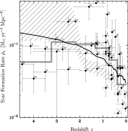
Figure 8: The global star formation rate according to Eq. (18), taken from simulations with box size $L_{\rm{box}}=80\,h^{-1}\>\mathrm{Mpc}$ (solid line). Depicted data points (cf. the compilation by Ascasibar et al., 2001) are from: Pascarelle et al. (1998, p), Steidel et al. (1999, m), Treyer et al. (1998, t), Lilly et al. (1996, l), Cowie et al. (1999, c), Connolly et al. (1997, n), Sawicki et al. (1997, w), Gallego et al. (1995, g), Tresse & Maddox (1998, d), Glazebrook et al. (1999, g), Yan et al. (1999, y), Flores et al. (1999, f), Hughes et al. (1998, h), Pascual et al. (2002, u), Tresse et al. (2002, e), Hopkins et al. (2000, k), Sullivan et al. (2000, v), Gronwall (1999, x), Moorwood et al. (2000, o), Hammer et al. (1997, r), and Haarsma et al. (2000, a). We applied the correction given by Ascasibar et al. (2001) to obtain star formation rates in the $\Lambda$CDM model. The solid gray line indicates the mean of the observed star formation rate. A quite different evolution is indicated by the data points given by Lanzetta et al. (2001) (hashed area).

For an appropriate description of the IGM in cosmological simulations the feedback of stars must be necessarily taken into account. Therefore, a prescription for the star formation rate per volume within simulations of the large-scale structure formation is needed.

As briefly reviewed in the introduction it is usually assumed that baryonic matter which fulfills certain density and temperature criteria is able to form stars according to the Schmidt-law being aware that this is an empirical law, based on much different conditions.

The ‘true’ conjunction between the available parameters in such simulations and star formation is still unknown and allows to speculate and to set up very different models. From detailed star formation models in turbulent MCs indications are provided that the star formation rate may be controlled by mechanisms which force interstellar turbulence. One possibility to stir the ISM may be the merging of galaxies or the occurrence of minor-mergers. Such merging events are supposed to generate efficient star formation (e.g. Kauffmann et al., 2001).

We have investigated the energy-injection into the internal motions of the halos at sizes of $\approx$ 30 kpc - 2 Mpc due to the large-scale structure formation and we have found that the energy per mass input is comparable with energy injection rates attributed to supernova. However, even if the energy transfer from the large-scale structure formation provides sufficient energy to stir the ISM, at present it cannot be shown neither a mechanism to propagate the injected energy down to scales of observed ISM turbulence nor the detailed structure of the necessary turbulent field (for addressing this problem see however Jog & Ostriker, 1988; Sellwood & Balbus, 1999). Although the effect of the energy transfer onto the ISM is unknown, it represents one of the possible sources for driving the interstellar turbulence. Therefore, we assume here that the energy input is the linking parameter and make the following proposition:

The energy transfer from the large-scale structure formation provides sufficient energy to stir the ISM and the transfer is the main energy source for interstellar turbulence. Then, as a consequence, the amount of star formation should be determined by this energy transfer as well.

Following this quite speculative conjunction we would like to construct a prescription for the star formation rate within a small volume still described within large-scale structure formation simulations, i.e. related to scales of a few kpc. We assume direct proportionality to the local energy injection rate $\pi_{K}^{>}({\boldsymbol{x}}_{i})\propto\partial_{t}\sum_{n\in i}\sigma_{n}^{2}$. For a given halo part of the kinetic energy of the gas is transformed into heat. High temperature is expected to suppress star formation. We make the crude assumption that the thermal energy is a constant fraction proportional to the kinetic energy of the halo gas. This leads us to assume inverse proportionality of the SFR to the energy already stored within the small-scale motions $e_{K}^{>}({\boldsymbol{x}}_{i})\propto\sum_{n\in i}\sigma_{n}^{2}$.

In the result we get for the fraction of mass which is transferred into stars during a certain time interval $\Delta t$ within a given cell ${\boldsymbol{x}}_{i}$

$$\frac{\Delta m_{\ast}({\boldsymbol{x}}_{i})}{m({\boldsymbol{x}}_{i})} = \epsilon_{0}\;\frac{\pi_{K}^{>}({\boldsymbol{x}}_{i})}{e_{K}^{>}({\boldsymbol{x}}_{i})}\Delta t$$ (18)

$$\propto \frac{\partial_{t}\sum_{n\in i}\sigma_{n}^{2}}{\sum_{n\in i}\sigma_{n}^{2}}\Delta t=\frac{\partial_{t}\langle\sigma_{n}^{2}\rangle_{\rm{cell}}}{\langle\sigma_{n}^{2}\rangle_{\rm{cell}}}\Delta t$$

where $\epsilon_{0}$ is a normalization constant which has to be determined, e.g. by the observed SFR at any fixed redshift, and $m({\boldsymbol{x}}_{i})$ denotes the mass within the considered cell. As can be seen from the last term in Eq. (18) the ratio $\pi_{K}^{>}/e_{K}^{>}$ is independent from the local density. The comoving cosmic SFR $\dot{\rho}_{\ast}$ is obtained by summing up the contributions of all cells and dividing by the comoving volume of the simulation box $L_{\rm{box}}^{3}$

$$\dot{\rho}_{\ast} = \frac{\sum_{i}\,\Delta m_{\ast}({\boldsymbol{x}}_{i})}{\Delta t\;L_{\rm{box}}^{3}}.$$ (19)

Note, assuming for the SFR proportionality to the local specific energy injection the expression (18) represents the simplest combination of quantities obeying the dimensional requirements.

Since the energy injection rate is closely correlated with the merging and the matter infall rates as was shown in an earlier section the star formation history calculated in this manner reflects mainly the influence of merging processes.

For transparency we give the time evolution of the different constituents of the expression (18) averaged over the comoving box volume, see Fig. 9. The amount of mass concentrated in regions with density contrast $\rho/\rho_{0}\geq 3$ increases continuously with time. The hierarchical clustering process leads to increasing kinetic energy of the halo matter which happens according to the mass inflow and concentration. This explains the quite similar slope for the density and kinetic energy evolution. The energy injection into small scales is a slightly decreasing function with time as shown already in the preceding section, cf. Fig. 4.

Implementing the prescription Eq. (18) within our simulations we obtain according to Eq. (19) the evolution of the cosmic star formation rate $\dot{\rho}_{\ast}$, as shown in Fig. 8. For comparison we included a compilation of observational data of star formation rates recently obtained for different redshifts. We have fixed the normalization constant $\epsilon_{0}$ using the data in the vicinity of $z=0.5$. Even if there is a big scatter in the estimated star formation rates it is commonly accepted that there is a steep increase from redshift zero to redshift one (cf. gray line). Estimates at higher redshift indicate a subsequent decline even if these measurements are still under debate. Although dust extinction is to some extend allowed for it may still cause the decline of the data points. A quite different star formation history is recently given by Lanzetta et al. (2001). They found a continuous increase of the SFR with redshift.

Figure 9: Evolution of the mean of the different constituents in the prescription Eq. (18), namely the mean of the variation of the local velocity dispersion $\partial_{t}\langle\sigma_{n}^{2}\rangle_{\rm{cell}}$, the amount of mass contained in regions with density contrast $\rho/\rho_{0}\geq 3$ (cf. Sec 4), and the mean of the local velocity dispersion $\langle\sigma_{n}^{2}\rangle_{\rm{cell}}$.

The evolution of the calculated ’star formation rate’ matches the cosmic star formation history to some extent. However, the limitations of the proposed model are obvious: In addition to the considered impact of energy transfer, which mainly reflects the impact of merging and accretion, the star formation is affected by hydrodynamical effects, radiation, etc. related to the properties of the baryonic matter. In particular, the back-reaction of the already formed stars onto the gas by winds, supernova etc. may locally turn off any subsequent star formation. These processes result almost exclusively in an reduction of star formation which may cause in particular a steeper slope at small redshifts than obtained here.

The advantage of the proposed quantity is obvious as well: It can be computed on-the-flight without determining the single matter halos and without tracing back their evolution. It can be used complementary within the framework of semi-analytical descriptions of star formation applied to the results of n-body simulations. Of course, this cannot replace the knowledge of the detailed star formation process including the full cooling history and detailed velocity fields. However, for the consideration of large-scale structure formation and the large scale distribution of quantities related to star formation this could serve as a suitable approximation.

8 Summary

During the formation of the large-scale structures gravitational energy is transferred into the internal motion of the dark matter halos. In particular by merging of the halos part of the kinetic energy is subsequently transferred from the large-scale movement into small-scale internal motions. The baryonic matter possesses the same amount of kinetic energy per mass as long as it moves together with the dark matter, i.e. as long as gravitational interaction dominates over pressure forces. Thus the large-scale structure formation is transferring energy into small scales. We have addressed the question how this transfer can be described, how it evolves during the cosmological structure formation and whether this transferred energy rate is of comparable order of magnitude to compete with internal energy sources in the galaxies.

We have performed cosmological n-body simulations to determine which energy amount the large-scale structure formation provides to a given small scale.

A crucial point in that picture is how the energy transfer is directed. We have considered this question investigating the evolution of the power spectrum of the large-scale velocity field. To this end we have used a method introduced by Lomb (1976). The power spectrum evolves according to the linear growth at scales larger $\approx 60\,h^{-1}\>\mathrm{Mpc}$. Below these scales it possesses a more shallow region and at scales below $\approx 0.5\,h^{-1}\>\mathrm{Mpc}$ it roughly behaves like a power law $\sim k^{-4.2}$. In general, the features of the velocity spectrum are similar to those of the power spectrum of the density field. The behavior of the velocity spectra shows that large-scale modes dominate the power of small-scale modes and that the energy transfer throughout the modes is almost exclusively one-directional, namely from larger to smaller scales.

To calculate the energy transfer through a given scale we have used the concept of cumulative energy. The Fourier transforms of the velocity field and of the density of momentum are subdivided into a high-pass and a low-pass filtered part. As a result the energy density can also be decomposed into a high-pass and a low-pass filtered part and the scale-by-scale energy budget contains a term describing the energy exchange between the two spectral ranges. The exchange rate may be calculated by help of the time derivative of the high-pass filtered energy and equals to the energy injection rate into scales smaller than the given cut-off length.

Using the involved quantities we can define straightforwardly the mean global energy exchange rate into given scales at any time during the performed n-body simulations. We obtain the mean energy exchange rate which increases with redshift according to a power law $\sim(z+1)^{3}$. We argue that this can be attributed to the mass increase of dark matter halos. The evolution includes all kinds of infall, i.e. continuous accretion of matter onto halos, minor mergers, or even merging of halos. If all processes evolve similar or if merging is dominant the evolution of the mean energy exchange exhibits the same time-dependence as the merging rate of dark matter halos.

Due to the additivity of the cumulative energy with respect to its local contributions if applied to grid based n-body systems a local high-pass filtered mean energy exchange rate can be defined supposing that the size of the local averaging volume is equal to the cut-off scale $\lambda_{K}$. A specific energy exchange rate is given by the ratio of the local energy exchange rate into a given volume to the local mass density. Using this definition we obtain the mean specific energy exchange rate which is as low as $\approx 10^{-28}\,n\>\mathrm{erg}\>\mathrm{s}^{-1}\>\mathrm{cm}^{-3}$. However, its expectation value is proportional to the density. Thus, in regions as dense as the galactic halo the energy input due to the energy exchange may be as large as $\approx 10^{-24}\,n\>\mathrm{erg}\>\mathrm{s}^{-1}\>\mathrm{cm}^{-3}$, which is comparable with the kinetic energy feedback by supernova averaged over the same galactic volume.

On the basis of our results we consider a speculative picture: We assume that the injected energy propagates to MC scales and is therefore available for driving the MC turbulence leading to star formation. On the ground of this quite heuristic assumptions we propose an estimator for the star formation rate in a local volume in cosmological simulations: $\dot{m}_{\ast}\propto(\pi_{K}^{>}/e_{K}^{>})\>m$.

The model reproduces approximately the observed global evolution of the star formation rate. Adopting this model means that merging and matter infall processes are considered to enhance the star formation at least or to be the leading processes.

References

- Ascasibar et al. (2001) Ascasibar, Y., Yepes, G., Gottlöber, S., & Müller, V. 2001, A&A, submitted
- Ballesteros-Paredes et al. (1999) Ballesteros-Paredes, J., Vázquez-Semadeni, E., & Scalo, J. 1999, ApJ, 515, 286
- Blitz et al. (1999) Blitz, L., Spergel, D. N., Teuben, P. J., Hartmann, D., & Burton, W. B. 1999, ApJ, 514, 818
- Blitz & Williams (1999) Blitz, L. & Williams, J. P. 1999, in NATO ASIC Proc. 540: The Origin of Stars and Planetary Systems, 3+
- Burkert (2001) Burkert, A. 2001, in 9 pages, 2 figures, conference proceeding. to appear in ”Modes of Star Formation”, eds. E.K. Grebel and W. Brandner, 5298+
- Carlberg et al. (1994) Carlberg, R. G., Pritchet, C. J., & Infante, L. 1994, ApJ, 435, 540
- Connolly et al. (1997) Connolly, A. J., Szalay, A. S., Dickinson, M., Subbarao, M. U., & Brunner, R. J. 1997, ApJ, 486, L11
- Cowie et al. (1999) Cowie, L. L., Songaila, A., & Barger, A. J. 1999, AJ, 118, 603
- Elmegreen (2000) Elmegreen, B. G. 2000, ApJ, 530, 277
- Flores et al. (1999) Flores, H., Hammer, F., Thuan, T. X., Césarsky, C., Desert, F. X., Omont, A., Lilly, S. J., Eales, S., Crampton, D., & Le Fèvre, O. 1999, ApJ, 517, 148
- Frisch (1994) Frisch, U. 1994, Turbulence: The Legacy of A. N. Kolmogorov (Heidelberg: Spetrum, Akad. Verlad)
- Gallego et al. (1995) Gallego, J., Zamorano, J., Aragon-Salamanca, A., & Rego, M. 1995, ApJ, 455, L1
- Glazebrook et al. (1999) Glazebrook, K., Blake, C., Economou, F., Lilly, S., & Colless, M. 1999, MNRAS, 306, 843
- Goldman (2000) Goldman, I. 2000, ApJ, 541, 701
- Gottlöber et al. (2000) Gottlöber, S., Klypin, A., & Kravtsov, A. V. 2000, preprint, astro-ph/0004132
- Gronwall (1999) Gronwall, C. 1999, in After the Dark Ages: When Galaxies were Young (the Universe at 2 ¡ z ¡ 5). 9th Annual October Astrophysics Conference in Maryland held 12-14 October, 1998. College Park, Maryland. Edited by S. Holt and E. Smith. American Institute of Physics Press, 1999, p. 335, 335+
- Haarsma et al. (2000) Haarsma, D. B., Partridge, R. B., Windhorst, R. A., & Richards, E. A. 2000, ApJ, 544, 641
- Hammer et al. (1997) Hammer, F., Flores, H., Lilly, S. J., Crampton, D., Le Fevre, O., Rola, C., Mallen-Ornelas, G., Schade, D., & Tresse, L. 1997, ApJ, 481, 49+
- Hopkins et al. (2000) Hopkins, A. M., Connolly, A. J., & Szalay, A. S. 2000, AJ, 120, 2843
- Hughes et al. (1998) Hughes, D. H., Serjeant, S., Dunlop, J., Rowan-Robinson, M., Blain, A., Mann, R. G., Ivison, R., Peacock, J., Efstathiou, A., Gear, W., Oliver, S., Lawrence, A., Longair, M., Goldschmidt, P., & Jenness, T. 1998, Nature, 394, 241
- Jog & Ostriker (1988) Jog, C. J. & Ostriker, J. P. 1988, ApJ, 328, 404
- Kauffmann et al. (2001) Kauffmann, G., Charlot, S., & Balogh, M. L. 2001, preprint, astro-ph/0103130
- Kauffmann et al. (1999) Kauffmann, G., Colberg, J. . M., Diaferio, A., & White, S. D. M. 1999, MNRAS, 307, 529
- Kay et al. (2001) Kay, S. T., Pearce, F. R., Frenk, C. S., & Jenkins, A. 2001, accepted for publication in MNRAS, astro-ph/0106462
- Kennicutt (1998) Kennicutt, R. C. 1998, ApJ, 498, 541+
- Klessen (2000) Klessen, R. S. 2000, ASP Conference Series, T. Montmerle & Ph. Andre, eds., preprint, astro-ph/0011224
- Klypin et al. (2000) Klypin, A., Kravtsov, A., & Colín, P. 2000, in ASP Conf. Ser. 201: Cosmic Flows Workshop, 344+
- Kolatt et al. (1999) Kolatt, T. S., Bullock, J. S., Somerville, R. S., Sigad, Y., Jonsson, P., Kravtsov, A. V., Klypin, A. A., Primack, J. R., Faber, S. M., & Dekel, A. 1999, ApJ, 523, L109
- Lanzetta et al. (2001) Lanzetta, K. M., Yahata, N., Pascarelle, S., Chen, H., & Fernandez-Soto, A. 2001, in 28 pages, 9 figures; accepted for publication in the Astrophysical Journal., 11129+
- Larson (2001) Larson, R. B. 2001, in Summary talk at the meeting on ”Modes of Star Formation and the Origin of Field Populations”, Heidelberg, Germany, October 2000; to be published in the ASP Conference Series, edited by E. K. Grebel and W. Brandner, 1046+
- Lilly et al. (1996) Lilly, S. J., Le Fevre, O., Hammer, F., & Crampton, D. 1996, ApJ, 460, L1
- Lomb (1976) Lomb, N. R. 1976, Ap&SS, 39, 447
- Mac Low et al. (1998) Mac Low, M.-M., Klessen, R. S., Burkert, A., & Smith, M. D. 1998, Phys. Rev. Lett., 80, 2754
- Moorwood et al. (2000) Moorwood, A. F. M., van der Werf, P. P., Cuby, J. G., & Oliva, E. 2000, A&A, 362, 9
- Nagamine et al. (2001) Nagamine, K., Fukugita, M., Cen, R., & Ostriker, J. P. 2001, ApJ, 558, 497
- Obukhov (1941) Obukhov, A. M. 1941, Izv. Akad. Nauk SSSR Ser. Geogr. Geofiz., 5, 453
- Padoan et al. (2001) Padoan, P., Juvela, M., Goodman, A. A., & Nordlund, Å. 2001, ApJ, 553, 227
- Pascarelle et al. (1998) Pascarelle, S. M., Lanzetta, K. M., & Fernández-Soto, A. 1998, ApJ, 508, L1
- Pascual et al. (2002) Pascual, S., Gallego, J., Aragon-Salamanca, A., & Zamorano, J. 2002, mNRAS, in press (astro-ph/0110177)
- Press et al. (1986) Press, W. H., Flannery, B. P., & Teukolsky, S. A. 1986, Numerical recipes. The art of scientific computing (Cambridge: University Press, 1986)
- Sawicki et al. (1997) Sawicki, M. J., Lin, H., & Yee, H. K. C. 1997, AJ, 113, 1
- Scalo & Biswas (2001) Scalo, J. & Biswas, A. 2001, MNRAS, accepted, (astro-ph/0111201)
- Scargle (1982) Scargle, J. D. 1982, ApJ, 263, 835
- Schmidt (1959) Schmidt, M. 1959, ApJ, 129, 243+
- Sellwood & Balbus (1999) Sellwood, J. A. & Balbus, S. A. 1999, ApJ, 511, 660
- Somerville et al. (2001) Somerville, R. S., Primack, J. R., & Faber, S. M. 2001, MNRAS, 320, 504+
- Springel (2000) Springel, V. 2000, MNRAS, 312, 859
- Steidel et al. (1999) Steidel, C. C., Adelberger, K. L., Giavalisco, M., Dickinson, M., & Pettini, M. 1999, ApJ, 519, 1
- Steinmetz (2001) Steinmetz, M. 2001, in ASP Conf. Ser. 230: Galaxy Disks and Disk Galaxies, 633–640
- Sullivan et al. (2000) Sullivan, M., Treyer, M. A., Ellis, R. S., Bridges, T. J., Milliard, B., & Donas, J. . 2000, MNRAS, 312, 442
- Timmes et al. (1997) Timmes, F. X., Diehl, R., & Hartmann, D. H. 1997, ApJ, 479, 760+
- Tresse & Maddox (1998) Tresse, L. & Maddox, S. J. 1998, ApJ, 495, 691+
- Tresse et al. (2002) Tresse, L., Maddox, S. J., Le Fevre, O., & Cuby, J.-G. 2002, mNRAS, submitted (astro-ph/0111390)
- Treyer et al. (1998) Treyer, M. A., Ellis, R. S., Milliard, B., Donas, J., & Bridges, T. J. 1998, MNRAS, 300, 303
- Yan et al. (1999) Yan, L., McCarthy, P. J., Freudling, W., Teplitz, H. I., Malumuth, E. M., Weymann, R. J., & Malkan, M. A. 1999, ApJ, 519, L47
- Yepes et al. (1997) Yepes, G., Kates, R., Khokhlov, A., & Klypin, A. 1997, MNRAS, 284, 235