The Canada-UK Deep Submillimeter Survey VI: The 3-Hour Field.

Abstract

We present the complete submillimeter data for the Canada-UK Deep Submillimeter Survey (CUDSS) 3^h  field. The observations were taken with the Submillimeter Common-User Bolometer Array (SCUBA) on the James Clerk Maxwell Telescope (JCMT) on Mauna Kea. The 3^h  field is one of two main fields in our survey and covers 60 square arc-minutes to a 3$\sigma$ depth of $\sim$ 3 mJy. In this field we have detected 27 sources above 3$\sigma$, and 15 above 3.5$\sigma$. We assume the source counts follow the form $N(S){\propto}S^{-\alpha}$ and measure $\alpha$ = 3.3${}^{+1.4}_{-1.0}$. This is in good agreement with previous studies and further supports our claim (Eales et al., 2000) that SCUBA sources brighter than 3 mJy produce $\sim$20% of the 850$\mu$m background energy. Using preliminary ISO 15 $\mu$m maps and VLA 1.4 GHz data we have identified counterparts for six objects and have marginal detections at 450$\mu$m for two additional sources. With this information we estimate a median redshift for the sample of 2.0$\pm$0.5, with $\sim$10% lying at $z<$ 1. We have measured the angular clustering of S_850μm  $>$ 3 mJy sources using the source catalogues from the CUDSS two main fields, the 3^h  and 14^h  fields, and find a marginal detection of clustering, primarily from the 14^h  field, of $\omega(\theta)=4.4\pm 2.9\theta^{-0.8}$. This is consistent with clustering at least as strong as that seen for the Lyman-break galaxy population and the Extremely Red Objects. Since SCUBA sources are selected over a broader range in redshifts than these two populations the strength of the true spatial clustering is expected to be correspondingly stronger.

1 Introduction

Over the last decade there have been great steps forward in our understanding of the formation and early evolution of galaxies. There are currently two general, distinct theories of massive galaxy formation, though the true picture is likely a combination of the two. In the first, galaxies form over a range of redshift, from the gradual hierarchical merging of smaller aggregates (Baugh, Cole, & Frenk, 1996; Kauffman & Cole, 1998). In this picture galaxy formation is an ongoing process characterised by star formation rates of moderate magnitude. In the second scenario galaxies form at high-redshift on short timescales from the collapse of a single object and undergo one massive burst of star formation (Eggen, Lynden-Bell, & Sandage, 1962). They then evolve passively to galaxies of the present-day.

The observational picture is still somewhat confused. Optical studies have found that the luminosity density of the universe increases out to z$\sim$1 (Lilly et al., 1996; Madau et al, 1998; Hogg et al., 1998) and, according to the observations of the Lyman-break galaxy population (LBG), does not decrease to at least z$\sim$4 (Steidel et al., 1999). However, the star formation rates in individual LBGs of a few tens of solar masses per year (Steidel et al., 1996), though large compared to local starbursts, are too moderate to form an elliptical galaxy on a dynamical timescale of $\sim$10⁸ years, and suggest gradual, hierarchical formation. The hierarchical model is further supported by the increase in the rate of galaxy-galaxy interactions with redshift (Patton et al., 2001).

On the other hand, the spheroids, which contain $\sim$2/3 of the stars in the universe (Fukugita, Hogan, & Peebles, 1998) still appear to be old at z$\sim$1 (Zeph, 1997; Cimatti et al., 1999; Scodeggio & Silva, 2000; Moriondo, Cimatti, & Daddi, 2000). The homogeneous nature of their stellar populations today (Bower, Lucey, & Ellis, 1992) imply formation over a short timescale and at high redshift. However, until recently, no high-redshift object with star formation rates large enough to form a massive spheroid in a dynamical timescale had been seen. The deep submillimeter surveys of the last five years, (Smail, Ivison & Blain, 1997; Hughes et al., 1998; Barger et al., 1998; Eales et al., 1999) with the Submillimeter Common-User Bolometer Array (SCUBA) on the James Clerk Maxwell Telescope (JCMT), have uncovered just such a population.

The results of these deep SCUBA surveys have been exciting and in general agreement with each other. The population revealed by the SCUBA surveys covers a broad range of redshift, with a median redshift of 2 $<$ z $<$ 3 (Eales et al., 2000; Dunlop, 2001). Many of the submillimeter detections which have secure optical/near-infrared (NIR) counterparts show disturbed morphology or multiple-components suggestive of galaxy mergers (Lilly et al., 1999; Ivison et al., 2000). These objects have spectral energy distributions broadly similar to today’s ultra-luminous infrared galaxy (ULIRG) population. In the local universe the ULIRGs are the most luminous galaxies and emit the bulk of their energy at FIR wavelengths. The FIR emission is from dust which is currently thought to be heated by young stars (Lutz et al., 1999).The ULIRGs are primarily the result of mergers and result in objects with surface-brightness profiles of elliptical galaxies (see Sanders & Mirabel (1996) for a review). Though the dust temperature of the SCUBA sources is very poorly known, if we assume a temperature similar to the local ULIRGS then these objects are extremely luminous, with bolometric luminosities of 10^12-13L_⊙. Radio and CO observations of two SCUBA sources (Ivison et al., 2001) have detected possible extended emission which is in marked difference to the compact nature of local ULIRGs. It is still unclear whether the majority of these objects are powered by star formation or active galactic nuclei (AGN). Evidence is mounting through X-ray and optical emission line measurements that, although AGN are present in a small fraction of sources, star formation is, by far, the dominant process (Ivison et al., 2000; Fabian et al., 2000; Barger et al., 2001). Given this, the ULIRGs must be forming stars at unprecedented rates of hundreds to thousands of solar masses per year (Ivison et al., 2000; Eales et al., 1999). These high star formation rates, together with the contribution that these objects make to the total extragalactic background, showing this is a cosmologically-significant population (Eales et al., 2000), makes it hard to avoid the conclusion that these objects are elliptical galaxies being seen during their initial burst of star formation.

Analysis of the spatial clustering of different populations can provide clues to their evolutionary connections. Recent measurements of the clustering of two other populations of high-redshift galaxies, the LBGs and Extremely Red Objects (EROs), (Giavalisco et al., 1998; Giavalisco & Dickinson, 2001; Daddi et al., 2000, 2001) have yielded surprising results. Studies of the z $<$ 1 universe (Le Fèvre et al., 1996; Carlberg et al., 2000) have found the clustering strength of galaxies to decrease with increasing redshift, as expected in a scenario where structure forms through gravitational instabilities. However, the LBGs ($z\sim$3) and the EROs ($z\mathrel{\hbox{\hbox to0.0pt{\hbox{\lower 4.0pt\hbox{$\sim$}}\hss}\hbox{$>$}}}$1) are very strongly clustered. With hindsight this result is in agreement with the prediction of Kaiser (1984) that the highest peaks in the density field of the early universe should be strongly clustered. At the redshifts of LBGs and EROs the universe was much younger and there had been less time for gravitational collapse. These objects are therefore probably the result of the collapse of the rare high peaks in the density field. As SCUBA sources are even rarer than the LBGs, and based on their star formation rates perhaps more massive, they would also be expected to show clustering.

Peacock et al. (2000) investigated the underlying structure in a submillimeter map of the Hubble Deep Field (Hughes et al., 1998), after removing all discrete sources above 2 mJy, and found no significant clustering of the underlying flux. However, the HDF area is small and much larger areas are needed to investigate the clustering of submillimeter sources. Of the current deep SCUBA surveys there are two blank-field surveys of significant size and with which a clustering measurement may be made: the “8 mJy survey” (Scott et al., 2001), and our own, the Canada-UK Deep Submillimeter Survey (CUDSS). The “8 mJy survey” has detected a clustering signal for $\hbox{S${}_{850{\mu}m}$ \ }>$ 8 mJy sources over an area of 260 arcmin². Our survey covers 100 arcmin² and reaches a deeper depth of 3 mJy.

This paper is the sixth of a series of papers on the CUDSS project and contains the complete submillimeter data of our 3^h  field. The submillimeter survey is now complete and the final catalogue contains 50 sources, 27 of which have been detected in the 3^h  field. Paper I (Eales et al., 1999) introduces the survey and initial detections; paper II (Lilly et al., 1999) discusses the first optical identifications; paper III (Gear et al., 2000) discusses the multi-wavelength properties of a particularly interesting and bright source, 14-A; paper IV (Eales et al., 2000) presents the nearly complete 14^h field submillimeter sample and discusses the mid-IR and radio properties of the sources; paper V (Webb et al., 2001) investigates the relationship between SCUBA sources and LBG galaxies in the CUDSS fields; and papers VII and VIII (Clements et al., in preparation; Webb et al., in preparation) will discuss the optical and near-IR properties of the entire sample.

This paper is laid out as follows: §2 describes the submillimeter observations, §3 discusses the data reduction and analysis techniques, §4 presents the source catalogue, §5 discusses the radio and ISO data, in §6 we discuss individual sources, in §7 we present the source counts, in §8 the clustering analysis is performed and the implications of these results are discussed in §9.

2 Submillimeter Observations

We observed 60 arcmin² of the Canada-France Redshift Survey (CFRS) 3^h  field over 25 nights from January, 1998 through July, 2001 with SCUBA on JCMT (Holland et al., 1999). These data are part of the larger Canada-United Kingdom Deep Submillimeter Survey which also includes a 50 arcmin² region in the CFRS 14^h  field and two deep 5.4 arcmin² regions in the CFRS 10^h  and 22^h  fields. Some of these observations are discussed in earlier papers (please see §1 for outline) and will be discussed futher in future papers. SCUBA is a system of two bolometer arrays which observe at 850$\mu$m and 450$\mu$m simultaneously. The beam sizes are roughly 15.0^′′ and 7.5^′′ at 850$\mu$m and 450$\mu$m respectively. Our data were taken using the “jiggle mode” of SCUBA which fully samples the sky plane through 64 offset positions.

The final image is a mosaic of of 101 overlapping individual jiggle-maps, ($\sim$ 50 minutes per jiggle-map). Each point in the final map contains data from about nine separate jiggle-maps, giving an effective total integration time of about 8 hours. Because a source will likely fall on different bolometers in different jiggle-maps, this procedure reduces the chance of spurious sources being produced by noisy bolometers. This mosaicing procedure also produces a fairly constant level of noise over a large area of sky.

We chose a “chop throw” of 30 arcsecs so that while chopping off-source an object will still fall on the array, except at the very edges of the map. We chopped in right ascension (RA) which creates a distinct pattern on the map for real objects of a positive source with two negative sources (at half the flux) offset by 30^′′ in RA on either side. In the map analysis this pattern is used to discriminate between real sources and spurious noise spikes which, unlike real objects will not be accompanied by two negative sources.

The opacity of the atmosphere was determined from “skydip” observations which were taken in between each single jiggle-map (approximately once every hour) except in exceptionally stable weather when skydips were taken every second jiggle-map. Observations to correct for pointing errors were done with the same frequency and pointing offsets were consistently less than 2 arcseconds. The observations were calibrated each night using Mars, Uranus, CRL618 or IRC+10216. Although IRC+10216 has long-term variability it has been recalibrated in 1998, and the variablility is much less than our expected calibration error at 850$\mu$m of approximately 10%.

3 Data Reduction and Source Extraction

The data reduction procedure is discussed in detail in Eales et al. (2000). We follow the standard SCUBA User Reduction Facility (SURF) reduction procedure (Jenness, 1997). First the “nod” is removed by subtracting the off-position data from the on-position data. Next, the maps are flat-fielded which removes the effects of sensitivity variations between the bolometers. We then correct for sky opacity using the ${\tau}_{850}$ and ${\tau}_{450}$ values determined from the skydips taken before and after each observation. The median sky value at each second is determined and removed from all the bolometers. This is done because in practice the chopping and nodding procedure used to remove the sky emission does not work perfectly for two reasons. First, the sky may vary faster than the chop frequency. Second, this procedure will only remove linear gradients in the sky brightness. Individual measurements from the time-series of each bolometer above 3$\sigma$ are then rejected from the data in iterative steps to reduce the noise. As our objects are faint, even after 8 hours of integration, we are not in danger of removing source flux in this step. The data from individual bolometers are weighted according to their noise and “rebinned” to construct a map. Figure 1 shows our final 850 $\mu$m map, smoothed with a 10^′′ Gaussian profile.

The map used for source extraction is produced by convolving this image with a beam template, which includes the negative beams as well as the postive beam. We produced this from the observations of our flux calibrators which are close to being point sources. This suppresses spurious sources (noise spikes) in the final map as they are not well matched to the negative-positive-negative pattern of the beam. Real sources, on the other hand, are well matched to the beam template and the flux in the negative beams is combined with the positive flux in the final convolved map, thereby increasing the signal-to-noise. This procedure will also produce a more accurate measurement of the position of the source since the positional information off all three beams is used.

SCUBA acquires data at 450$\mu$m and 850$\mu$m simultaneously and so the 450$\mu$m data, though significantly less useful than the 850$\mu$m data because of the increased sky noise and decreased sky transparancy, comes for free. The 450$\mu$m data was reduced in the same way as the 850$\mu$m data and the map was convolved with the beam template. The template-convolved map is shown in Figure 2.

We generated maps of the noise through Monte Carlo simulations, as described in paper IV. For each jiggle-map data set, we determined the standard deviation of the time-stream for each bolometer, and then replaced the time-stream with artificial data with the same standard deviation. We implicitly assumed that the real time-stream has a Gaussian distribution and that the noise on different bolometers was uncorrelated.

The artificial time-stream does not have quite the same distribution as the real time-stream, partly because the reduction procedure gets rid of points more than 3$\sigma$ from the mean. To simulate this effect, we applied the reduction procedure to the artificial time-stream, and then re-scaled the result so it again had the same standard deviation as the real time-stream. In this way we produced 500 simulated maps and the final noise map (Figure 3) was generated from the standard deviation of each pixel in these maps.

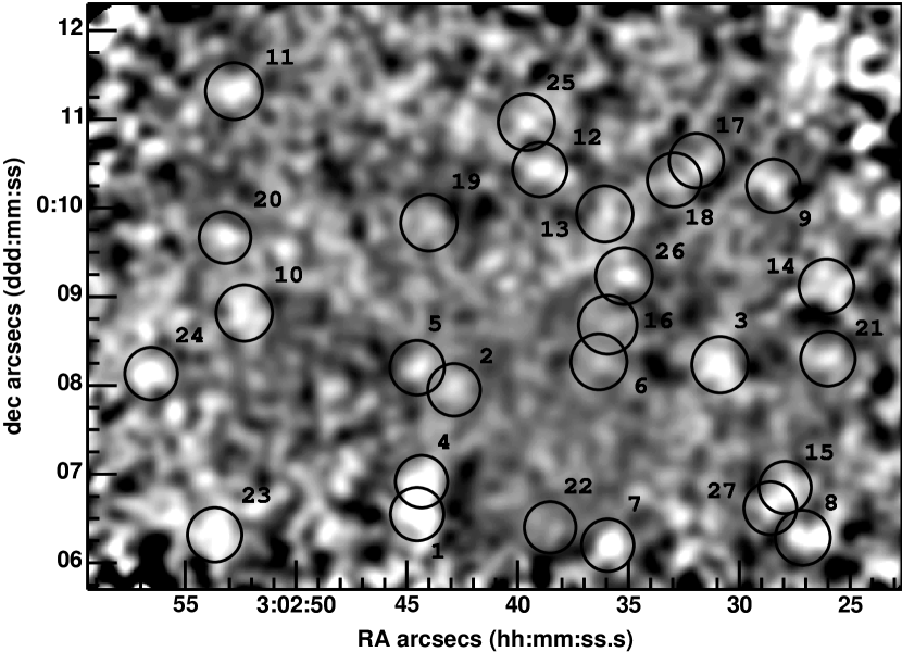
Figure 1: The 850 $\mu$m map smoothed with a 10^′′ Gaussian. Object numbers correspond to those in Table 1 and are ordered according to according to signal-to-noise.

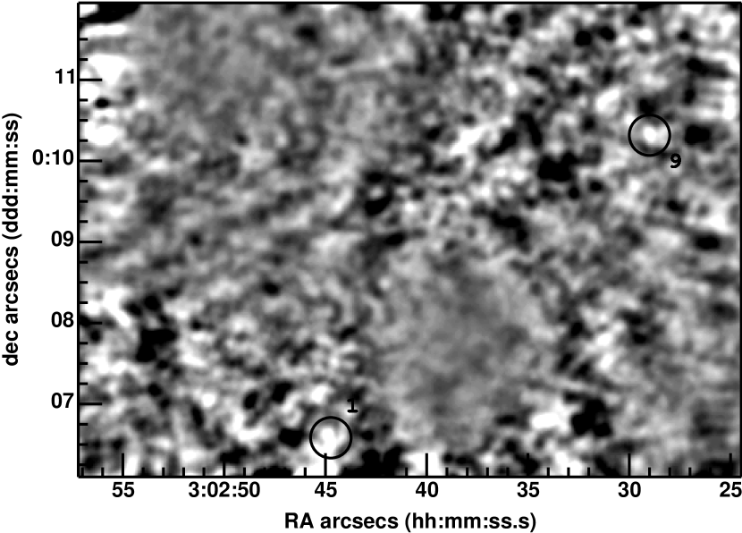
Figure 2: The 450 $\mu$m map convolved with the beam template. The atmospheric interference at 450$\mu$m is much worse than at 850$\mu$m and the noise pattern is therefore much more obvious. We show the the template-convolved map since it suppresses the noise spikes and the two 450$\mu$m detections of 850$\mu$m sources are more obvious to the reader than in a simple Gaussian smoothed map.

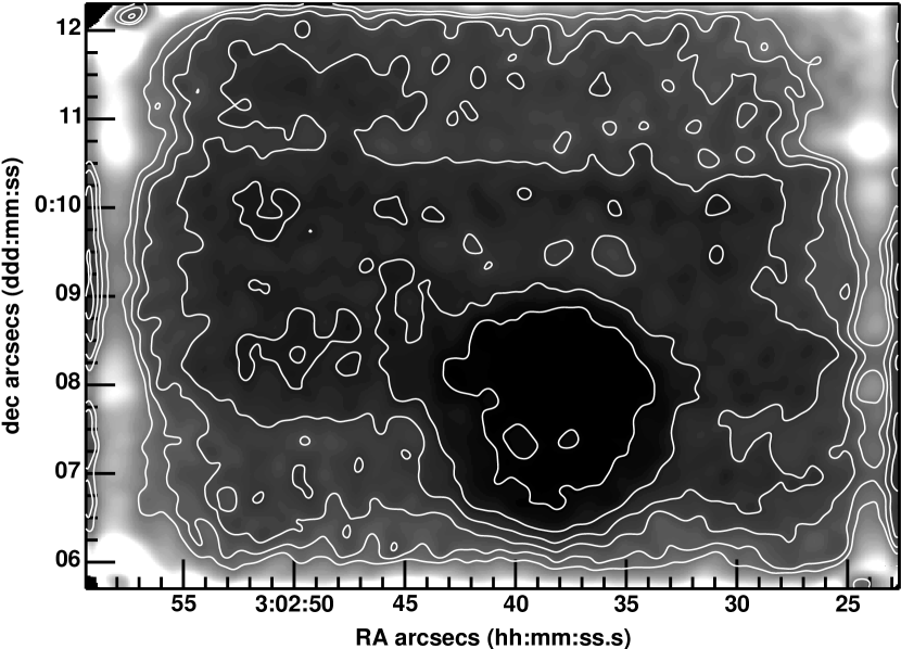
Figure 3: The 850 $\mu$m noise map. The contours begin at 0.75 mJy and increase in 0.25 mJy increments to 2.0 mJy. The non-uniform sensitivity across the field is clearly visible and is due primarily to weather, though the top-most strip has less time coverage. The single deep pointing was done in superb weather conditions.

Due to varying weather conditions our 3^h map is not as uniformly sampled as our 14^h map (paper III) and this is clearly visible in Figures 2 and 3. Most striking is the single deep pointing (2.7^′ across) which was taken in early 1998. The noisy edge effects are also seen and a well understood effect of SCUBA’s mapping technique. The center strip of the map was observed during excellent conditions while the remaining top and bottom strips under more marginal conditions and the top strip has incomplete coverage. Ignoring the noisy edge the map may be broken into 3 general sections:

1. the central deep pointing: mean 1$\sigma$ noise = 0.77 mJy

2. the central strip: mean 1$\sigma$ noise= 1.1 mJy

3. the top and bottom strip : mean 1$\sigma$ noise=1.4 mJy

4 The Catalogue

The source extraction was performed on the map which had been convolved with the beam template and then divided by the noise map, giving a signal-to-noise map. The extraction procedure is quite complicated because not only do many of the peaks in the map have low signal-to-noise, they are often merged together. We used the iterative de-convolution (CLEANing) technique described in Paper IV to compile a source catalogue.

The data reduction, source extraction, and noise analysis were performed separately and in parallel by the Cardiff and Toronto groups and the final source lists compared. Sources were included in the catalogue if their Cardiff-Toronto average signal-to-noise was above 3$\sigma$. The complete 3^h  catalogue is presented in Tables 1 and 2. There are 27 objects in total which were detected above 3$\sigma$. Sources which were less than 3$\sigma$ in one of the maps (but averaged above 3$\sigma$) are noted. Also listed are offsets in the Cardiff-Toronto averaged recovered positions.

We used the signal-to-noise map to investigate the number of spurious sources. Since the noise is symmetric around zero the number of peaks in the inverted map above a given signal-to-noise will be indicative of the number of spurious positive sources. This number becomes large below 3$\sigma$. Above the 3$\sigma$ threshold there are 2 negative sources, (both $<$ 3.5$\sigma$) indicating that about this number of our positive detections are spurious. This analysis was done after the CLEANing procedure was complete and full beam profile of the positive sources in the map removed. Therefore the negative sources at $>$ 3$\sigma$ which are not spurious but are associated with real positive peaks are not included in this analysis. The number of spurious sources is approximately the number expected from Gaussian statistics.

We define two catalogue lists: the primary list containing 15 objects above 3.5$\sigma$ which we regard as secure sources and the secondary list containing 12 objects between 3.5$\sigma$ and 3.0$\sigma$ which are more dubious. Based on the above reasoning we expect approximately 2 objects in the secondary list to be spurious detections.

Also listed in Tables 1 and 2 are the 450$\mu$m flux measurements and 3$\sigma$ upper limits for each source, measured at the 850$\mu$m position on the 450$\mu$m map. We searched for 450$\mu$m flux in two ways. First, we used the 450$\mu$m map which had been convolved with the beam and searched for $>$3$\sigma$ peaks within the error radius of the 850$\mu$m position. This gave us a list of possible 450$\mu$m detections. To test the robustness of these detections we performed aperture photometry on the unconvolved map as in Dunne & Eales (2001). Sources which had consistent flux measurements from both these methods were taken as real detections. There were two such sources corresponding to sources 3.1 and 3.9. This is consistent with the 450$\mu$m number counts presented in Blain et al. (1999). As the beam of the JCMT is smaller at 450 $\mu$m (7^′′ FWHM) the position of the 450$\mu$m peak flux is expected to be a better estimate of the true position of the source than at 850$\mu$m and should aid in optical/near-IR identifications.

Table 1: The 3^h Source List: Objects with S/N $\geq$ 3.5

Name	R.A. (2000.0)	Declin. (2000.0)	S/N	S850μm(mJy)	S450μm(mJy)	Positional Offset (arcsecs)
					(3$\sigma$ upper limits)	Cardiff-Toronto ($\prime\prime$)
CUDSS 3.1	03 02 44.55	00 06 34.5	7.4	10.6$\pm$1.4	83$\pm$26 (6.3)	1.8
CUDSS 3.2	03 02 42.80	00 08 1.50	6.7	4.8$\pm$0.7	$<$57	1.0
CUDSS 3.3	03 02 31.15	00 08 13.5	6.4	6.7$\pm$1.0	$<$63	1.8
CUDSS 3.4	03 02 44.40	00 06 55.0	6.2	8.0$\pm$1.3	$<$78	0.0
CUDSS 3.5	03 02 44.40	00 08 11.5	5.8	4.3$\pm$0.7	$<$57	1.0
CUDSS 3.6	03 02 36.10	00 08 17.5	5.4	3.4$\pm$0.6	$<$33	1.0
CUDSS 3.7	03 02 35.75	00 06 11.0	5.3	8.2$\pm$1.5	$<$63	1.5
CUDSS 3.8	03 02 26.55	00 06 19.0	5.0	7.9$\pm$1.6	$<$63	1.5
CUDSS 3.9	03 02 28.90	00 10 19.0	4.6	5.4$\pm$1.2	76.9$\pm$25 (0)	0.0
CUDSS 3.10	03 02 52.50	00 08 57.5	4.5	4.9$\pm$1.1	$<$57	1.0
CUDSS 3.11	03 02 52.90	00 11 22.0	4.0	5.0$\pm$1.3	$<$36	1.5
CUDSS 3.12	03 02 38.70	00 10 26.0	4.0	4.8$\pm$1.2	$<$75	0.0
CUDSS 3.13	03 02 35.80	00 09 53.5	3.8	4.1$\pm$1.1	$<$75	3.2
CUDSS 3.14	03 02 25.78	00 09 7.50	3.5	5.1$\pm$1.5	$<$63	1.8
CUDSS 3.15	03 02 27.60	00 06 52.5	3.5	4.4$\pm$1.3	$<$63	1.0

Table 2: The 3^h Source List: Objects with 3.5 $>$ S/N $\geq$ 3.0

Name	R.A. (2000.0)	Declin. (2000.0)	S/N	S850μm(mJy)	S450μm(mJy)	Positional Offset
					(3$\sigma$ upper limits)	Cardiff-Toronto ($\prime\prime$)
CUDSS 3.16	03 02 35.90	00 08 45.0	3.4	2.8$\pm$0.8	$<$63	3.0
CUDSS 3.17	03 02 31.65	00 10 30.5	3.4	5.0$\pm$1.5	$<$75	1.8
CUDSS 3.18	03 02 33.15	00 10 19.5	3.3	3.9$\pm$1.2	$<$75	1.8
CUDSS 3.19	03 02 43.95	00 09 52.0	3.2	3.3$\pm$1.0	$<$57	1.5
CUDSS 3.20	03 02 53.30	00 09 40.0	3.2	3.4$\pm$1.1	$<$57	2.0
CUDSS 3.21	03 02 25.90	00 08 19.0	3.1	3.8$\pm$1.2	$<$63	0.0
CUDSS 3.22	03 02 38.40	00 06 19.5	3.1	3.1$\pm$1.0	$<$33	1.0
CUDSS 3.23	03 02 54.00	00 06 15.5	3.1	5.8$\pm$1.9	$<$78	3.2
CUDSS 3.24	03 02 56.80	00 08 8.00	3.0	5.1$\pm$1.7	$<$60	3.0
CUDSS 3.25	03 02 38.65	00 11 12.0	3.0	4.1$\pm$1.4	$<$75	2.5
CUDSS 3.26	03 02 35.10	00 09 12.5	3.0	3.6$\pm$1.2	$<$75	1.0
CUDSS 3.27	03 02 28.56	00 06 37.5	3.0	4.0$\pm$1.3	$<$63	3.4

5 The Radio and ISO Data

We obtained a shallow VLA map of the field at 1.4 GHz with the B-array (Yun et al., in preparation) and a preliminary ISO 15$\mu$m map of Flores and collaborators (Flores et al., in preparation). To identify possible associations between the SCUBA sources and ISO and radio objects we used the same positional probability analysis as we use for the optical and near-IR data (Lilly et al., 1999). The probability that an unrelated ISO or radio source will lie within a distance $r$ of a given SCUBA position can be described by $P=1-exp(-\pi nr^{2})$, where $n$ is the surface density of the ISO or radio sources. Our Monte-Carlo analysis (Eales et al., 2000) implies that the true position of a SCUBA source will lie within 8^′′ of the measured position 90-95% of the time, and we therefore looked for ISO and radio sources within this distance of each SCUBA source. Because the surface density of ISO and radio sources is small, we do not expect many chance associations even with such a large search radius. The results are given in Tables 3 and 4.

The source with the largest $P$ value (determined from the radio data) is CUDSS 3.8, because of the very large offset between the radio position and the SCUBA position. In a sample of this size, we would expect about one source to have such a $P$ value, due purely to chance coincidence. However, the two other objects with radio detections have such small $P$ values that we may regard them a secure identifications. For the six sources with ISO detections CUDSS 3.8 is also the least secure, again because of its large offset from the submillimeter position. Source CUDSS 3.27 is also an insecure identification because we would expect at least one such coincidence in our sample, and it also lacks supporting data, such as a radio detection. However, given the $P$ values of the remaining four ISO identifications we would expect at most one chance coincidence and we therefore regard these identifications as secure (in particular the ones also identified with a radio source).

Table 3: Radio Associations

CUDSS	Flux ($\mu$Jy)	offset to SCUBA	P
		position (arcseconds)
CUDSS 3.8	746 $\pm$ 14	9.0	0.023
CUDSS 3.10	119 $\pm$18	1.3	0.00061
CUDSS 3.15	188 $\pm$ 20	2.3	0.0019

Table 4: ISO Associations

CUDSS name	ISO name	$S_{15{\mu}m}$ ($\mu$Jy)	offset to SCUBA	P
			position (arcseconds)
CUDSS 3.8	1003	1480	9.6	0.22
CUDSS 3.10	425	825	1.5	0.00087
CUDSS 3.15	1040	254	3.2	0.027
CUDSS 3.22	770	335	7.5	0.021
CUDSS 3.24	382	181	2.1	0.0017
CUDSS 3.27	1039	174	6.7	0.11

6 Notes on Individual Sources

Below we discuss individual sources with detections at ISO, radio, and 450$\mu$m wavelengths, and sources with Cardiff-Toronto positional offsets of $>$2^′′ . The optical and near-IR identifications are discussed in detail in Clements et al. (in preparation).

CUDSS 3.1

This is the brightest object in both the 3^h  and 14^h  catalogues. It is detected at 450 $\mu$m which would suggest it is at low redshift. This agrees with a possible optical ID, CFRS 03.0982 (Clements et al., in preparation), which has a spectroscopically determined redshift of z=0.1952 (Hammer et al., 1995). This source is located near the edge of the field and highly confused with CUDSS 3.4 as well as a third possible 850$\mu$m source at $<$ 3$\sigma$ and so the position is likely to be uncertain. The new 450$\mu$m position increases the offset to CFRS 03.0982 from 4^′′ to 7^′′ , but it remains the best optical/near-IR identification. However, there are two facts which suggest this is not the correct identification. First the probability that CFRS 03.0982 is unrelated to the SCUBA source is quite large (Clements et al. in preparation). Second, if this object does indeed have a redshift of $z$ = 0.1951 it should certainly be detected at 1.4 GHz, given its 450$\mu$m and 850$\mu$m fluxes, which it is not.

CUDSS 3.8

This is one of three detected in our shallow 1.4 GHz map and one of six detected with ISO at 15$\mu$m (ISO source 1003). The optical counterpart CFRS 03.0358 has a spectroscopic redshift of $z$=0.0880 (Hammer et al., 1995). The identification offset of 9^′′ is the largest for our sample but the radio and ISO detections and clear merger morphology in the optical image (Clements et al., in preparation) secures the identification. There is no 450$\mu$m detection but this is not entirely surprising since the object lies very near the edge of the smaller 450$\mu$m map where the noise is high.

CUDSS 3.9

This object is one of two detected at 450$\mu$m which suggests it is a low-redshift. However, there is no galaxy visible within 8^′′ of the SCUBA position in deep optical and near-IR images.

CUDSS 3.10

This object is identified with ISO source 425 with an offset of 1.5^′′ . The optical image shows a very bright galaxy (CFRS 03.1299, $I_{AB}$=19.4) with clear merger morphology. It has a spectroscopic redshift of $z$=0.176.

CUDSS 3.13

The Toronto-Cardiff positions disagree by 3.2^′′ likely because this source is extended and may therefore be two sources confused together.

CUDSS 3.15

This is identified with ISO source 1040 with an offset of 3.2^′′ . The optical identification CFRS 03.0346, is a bright ($I_{AB}$=22.1) galaxy with no unusual morphology.

CUDSS 3.16

The Toronto-Cardiff positions disagree by 3.0 arcsecs, likely due to its faintness.

CUDSS 3.22

This is identified with ISO source 770, which is CFRS 03.1029.

CUDSS 3.23

The Toronto-Cardiff position disagree by 3.2^′′ . This object is near the edge of the map, where the noise increases rapidly, and is below 3$\sigma$ in one of the Toronto-Cardiff catalogues.

CUDSS 3.24

This source is very close to the edge of the map and has a Toronto-Cardiff positional disagreement of 3.0^′′ . It is identified with ISO source 382, which is coincident with a red ($(I-K)_{AB}>$ 3.0) galaxy.

CUDSS 3.27

The Toronto-Cardiff positional disagreement for this source is 3.4^′′ (the largest disagreement in the catalogue) which is not surprising since this source is the faintest of a trio of confused sources including CUDSS 3.15 and CUDSS 3.8. This object is identified with ISO source 1039, which is CFRS 03.0338. Note that all three sources in this trio are identified with ISO sources, and one has a radio detection.

7 The Source Counts

We present the integral source counts from these data in Figure 4. They are in good agreement with the results of other surveys (Blain et al., 1999; Borys et al., 2001; Scott et al., 2001). To fit the counts we assumed they followed the form $N(>S)=N_{\circ}S^{-{\alpha}}$ and used the maximum likelihood technique outlined in Crawford et al. (1970) to determine $\alpha$. We find $\alpha$=3.3${}^{+1.4}_{-1.0}$ for the differential counts ($N(S)\propto S^{-\alpha})$, where the errors are 95% confidence limits. This is in excellent agreement with result of $\alpha$=3.2${}^{+0.6}_{-0.7}$ from Barger, Cowie & Sanders (1999). In Paper IV we investigated the effects of confusion and noise on the source counts and concluded that the slope is unaffected, though the counts are shifted upwards through flux-boosting.

In Figure 5 we plot the 3^h  and 14^h  (Eales et al., 2000) counts. For the 14^h  field we have included four new sources which were not part of our catalogue in Eales et al. (2000). Since that paper we have acquired additional 14^h  field data and these new sources will be discussed in detail in Webb et al. (in preparation). Although there are more bright objects in the 3^h  field we see no evidence for a different slope. Using the same fitting technique we measure $\alpha$=3.7${}^{+1.3}_{-1.1}$ for the differential counts for the 14^h  field. We note that there was a mistake in the source count analysis of the 14^h  field in Eales et al. (2000). However, the conclusion of Eales et al. (2000) that SCUBA sources brighter than S${}_{850{\mu}m}>$ 2mJy contribute $\sim$20% to the background at 850$\mu$m is unchanged by this new data and the new analysis.

Figure 4: The S_850μm source counts determined by different authors. The Diamonds correspond to (Scott et al., 2001), the asterisks to (Borys et al., 2001), the squares to (Blain et al., 1999), and the triangles to this work using the 3 hour field data.

Figure 5: The S_850μm source counts of the two CUDSS fields. The triangles correspond to the 3-hour field and the squares to the 14-hour field. Although there are more bright sources in the 3-hour field the slopes of the counts are consistent with each other.

8 The Angular Distribution of SCUBA Sources

We measured the angular correlation function for the SCUBA sources in the two fields, largely following the procedure given in Roche & Eales (1999). To estimate $\omega(\theta)$ we used the Landy & Szalay (1993) formalism:

$$\omega(\theta)={DD-2DR+RR\over RR}$$

where $DD$ is the number of SCUBA pairs at a given separation, $\theta$, $DR$ is the number of SCUBA-random pairs, and $RR$ is the number of random-random pairs, all normalized to the same number of objects. The Landy & Szalay approach is believed to have good statistical properties when a small correlation is expected.

To form $DR$ and $DD$ a sample of 5000 artificial SCUBA sources was generated, carefully taking into account sensitivity variations in the images. To do this we generated a set of random positions on the assumption of uniform sensitivity across the map. We then randomly assigned fluxes to these position using the best power-law fit to the source counts (§7). Using the noise maps (§3) (Eales et al., 2000) we determined whether each artificial source would be detected at $>$3$\sigma$ and thereby modeled the variation in source density across the SCUBA images.

The correlation analysis is further complicated by the shape of the beam. There will be no sources within $\sim$17 arcsecs since at this distance objects will be confused, but the effect of the beam actually extends over separations of $\sim$50 arcseconds in the RA direction (but not in Dec.) due to the chop. Sources can be detected in this area but the likelihood is decreased. To correct for this we placed masks around each SCUBA source corresponding to the shape of the beam. The number density of random sources around each SCUBA source thus more properly reflects the data. We calculated ${\omega}({\theta})$ for the entire sample as well separately for each field.

A final complication is that of the “integral constraint”. If $w(\theta)$ is estimated from an image, the integral

$${1\over\Omega^{2}}\int\int w_{est}(\theta)d\Omega_{1}d\Omega_{2}$$

will necessarily be approximately zero, even though the same integral of the true correlation function will not be zero for any realistic image size (Groth & Peebles, 1977). As in Roche & Eales (1999) we assumed the observed angular correlation is given by:

$$\omega(\theta)=A(\theta^{-0.8}-C)$$

and C is calculated from:

$$C={\sum\theta^{-0.8}_{ij}\over N_{r_{l}}N_{r_{s}}}$$

For the 14^h  and 3^h  fields we measure this to be 0.0106 and 0.0104 respectively.

Figure 6 shows our estimates of w($\theta$) for both the 3-hour and the 14-hour field and the combined results where the errors are estimated following Hewett (1982):

$$\delta\omega(\theta)^{2}={1+\omega(\theta)\over N_{p}}$$

A visual inspection of the angular distribution of sources in the 14^h  field (Eales et al., 2000) immediately suggests clustering, while the 3^h  field appears more uniformly distributed, and this is reflected in the correlation function measurement. We detect clustering in the 14^h  field, but not the 3^h  and the clustering detection remains when data from both fields are combined.

Fitting the data for the amplitude we measure $A$=2.4 $\pm$ 4.0 arcsec^0.8 for the 3 hour field, $A$=6.6 $\pm$ 4.2 arcsec^0.8 for the 14 hour field and $A$=4.4 $\pm$ 2.9 arcsec^0.8 for the combined data. These two fields are small enough that variance from field to field is expected to be important, so this discrepancy is not surprising. It should be noted though, that the 14^h  field, in which we detect marginal evidence for clustering, has very uniform noise properties (due to excellent weather). The clustering signal in the 3^h  field may have been washed out by the variations in sensitivity across the map which are much more extreme than for the 14^h  field.

Figure 6: The angular correlation function of SCUBA sources. The open circles correspond to the 14-hour field, the filled circles correspond to the 3-hour field and the open triangles correspond to the two fields combined. The solid line is the angular correlation function fit to the combined data. The dashed line is the angular correlation function of Lyman-break galaxies from Giavalisco et al. (1998) ($\omega(\theta)$=2${\theta}^{-0.9}$) and the dotted line is the angular correlation function of EROs (Daddi et al., 2000) ($\omega(\theta)$=5.8${\theta}^{-0.8}$).

Clustering information could, in principle, be gained from the difference in the number density of the two fields. The fractional error for the integral source counts for both fields is smallest for sources with flux densities greater than 3.5 mJy. We estimated the true surface density of objects from the average surface density of sources in the two fields. Using this value the difference in the number counts of the two fields is within the shot noise and is not indicative of clustering. Still, it does not rule it out since with such small field sizes shot noise is expected to dominate.

9 Discussion

9.1 The nature and redshift distribution of SCUBA sources

Determining the redshift distribution of the SCUBA population has proven difficult for two reasons: (1) determining the optical/near-IR counterpart is not trivial because of the large beam size of the JCMT at 850$\mu$m and (2) the inherent faintness of these sources at optical and near-IR wavelengths make spectroscopy difficult. Consequently, photometric redshift estimates, using a range of wavelengths, offer the best alternative. For the sources presented in this paper we have spectroscopic redshifts for 3/27 and the 450$\mu$m, 1.4 GHz, and ISO data provide further redshift information.

The 450$\mu$m to 850$\mu$m flux ratio can be used as a rough redshift estimate, though it is highly dependent on the shape of the spectral energy distribution (SED). In Figure 7 we show the 450$\mu$m to 850$\mu$m flux ratios for these objects as a function of redshift. We include the 450$\mu$m detections from the 3^h  and 14^h  fields and upper-limits from the 3^h  field only. The optical counterparts of sources 3.1, 3.8, and 3.10 have spectroscopic redshifts from the Canada-France Redshift Survey (though, we regard 3.1, with caution) and for the remaining sources (except 3.15 which has a radio detection) we estimated redshift lower-limits from their non-detection at 1.4 GHz (Carilli & Yun, 1999, 2000; Dunne, Clements, & Eales, 2000). Overlaid are the SEDs of three template galaxies. The solid line corresponds to Arp 220, the archetypal local ULIRG, the dashed line to a reddened starburst galaxy (which has less extinction than a ULIRG) and the dotted line to the more extreme object, IRAS 10214+4724. To estimate the reddened starburst SED we used the tabulated values of Schmitt et al. (1997) and extended the spectrum to wavelengths larger than 60$\mu$m assuming a dust temperature of 48K and a dust-emissivity index of 1.3, a good fit to the starburst galaxy M82. For IRAS 10214+4724 we assumed a temperature of 80K and a dust-emissivity index of 2 (Downes et al., 1992).

The 450$\mu$m to 850$\mu$m ratio for all three galaxy types drops very rapidly beyond a redshift of $z\sim$1-2 as the observed 450$\mu$m flux approaches the peak of the thermal flux. Thus, a detection at 450$\mu$m is indicative of either a low-redshift or very bright object. However, the ratio is highly dependent on temperature and the dust emissivity index and therefore, in the absence of SED information loses its power as a precise redshift indicator.

In Paper III we found the S_450μm/S_850μm upper-limits for the 14^h  field sources were just consistent with the IRAS 10214+4724 SED but always consistent with a reddened starburst and Arp 220. For the sources in the 3^h  field with estimated redshifts $z>1$ and S_450μm/S_850μm upper-limits we find a similar result, except for source 3.9 which has an exceptionally high S_450μm/S_850μm ratio, given its redshift lower-limit. As in Paper III we measure the mean 450$\mu$m to 850$\mu$m flux ratio from the mean 450$\mu$m flux all sources in the catalogue and find a 3$\sigma$ upper-limit of S_450μm/S_850μm = 2.6. This is considerably lower than for those objects detected at 450$\mu$m (which were included in the estimate) and is most consistent with SED’s similar to Arp 220 and the dusty starburst at redshifts of $z>$ 2.

We have detected six of the sources at 15$\mu$m with ISO, including sources 3.8, 3.10, and 3.15 which are also detected in the radio. The 15$\mu$m to 850$\mu$m flux ratio is a much stronger function of redshift than the 450$\mu$m to 850$\mu$m ratio (Figure 8) beyond $z\sim$ 0.5 but is also highly SED dependent. For sources 3.8 and 3.10, which have spectroscopic redshifts, $S_{15{\mu}m}/S_{850{\mu}m}$ ratio is lower than found for both the dusty starburst and Arp 200. However, the remaining four ISO detections appear to have higher ratios than expected for these SEDs if they lie at redshifts greater than $z\sim$3. At $1.0<z<3.0$ they are consistent with both Arp 220 and a dusty starburst.

The redshift information is listed in Table 5. All redshift lower-limits are derived from the radio/submillimeter flux ratio relation (Dunne, Clements, & Eales, 2000; Carilli & Yun, 2000). The redshift upper-limits are based on a detection at 450$\mu$m or 15$\mu$m. We estimated a mean redshift for the entire 3^h  sample using the routine ASURV (Feigelson & Nelson, 1985) and find $\overline{z}$=2.0$\pm$0.5. This value, and its uncertainty, was determine using both the lower-limit and upper-limit information (separately) and contains only three actual redshift measurements. We therefore regard it with caution. Though it is the lowest mean redshift measured by the SCUBA blank-field surveys, it is certainly in line with these estimates (Dunlop, 2001) and with our previous estimate from the initial 14^h  field data of 2.05$\pm$0.15 (Eales et al., 2000).Other blank-field surveys have claimed only 10% of the objects lie below $z\sim$ 2 (Dunlop, 2001). It is difficult to estimate the number of sources with $z<$ 2 in our sample, however, as we have 3/27 or $\sim$ 10% at $z<$ 1 the number below $z\sim$ 2 is likely much higher given the mean redshift estimate.

Table 5: Redshift Estimates for 3^h  Field Sources

CUDSS name	Redshift	Detection Wavelengths
CUDSS 3.1	0.1952	450$\mu$m
CUDSS 3.2	$>$ 1.4	–
CUDSS 3.3	$>$ 1.6	–
CUDSS 3.4	$>$ 1.7	–
CUDSS 3.5	$>$ 1.3	–
CUDSS 3.6	$>$ 1.7	–
CUDSS 3.7	$>$ 1.7	–
CUDSS 3.8	0.0880	1.4 GHz, 15$\mu$m
CUDSS 3.9	1.4 $<z<$ 3.0	450$\mu$m
CUDSS 3.10	0.176	1.4 GHz,15$\mu$m
CUDSS 3.11	$>$ 1.4	–
CUDSS 3.12	$>$ 1.4	–
CUDSS 3.13	$>$ 1.3	–
CUDSS 3.14	$>$ 1.4	–
CUDSS 3.15	1.3 $<z<$ 3.0	1.4 GHz, 15$\mu$m
CUDSS 3.16	$>$ 1.1	–
CUDSS 3.17	$>$ 1.4	–
CUDSS 3.18	$>$ 1.2	–
CUDSS 3.19	$>$ 1.2	–
CUDSS 3.20	$>$ 1.2	–
CUDSS 3.21	$>$ 1.2	–
CUDSS 3.22	1.1 $<z<$ 3.0	15$\mu$m
CUDSS 3.23	$>$ 1.5	–
CUDSS 3.24	1.4 $<z<$ 3.0	15$\mu$m
CUDSS 3.25	$>$ 1.3	–
CUDSS 3.26	$>$ 1.2	–
CUDSS 3.27	1.3 $<z<$ 3.0	15$\mu$m

Figure 7: The ratio of 450$\mu$m to 850$\mu$m flux as a function of redshift for the objects detected at 450 $\mu$m in the 3^h  , 14^h  , and 10^h  fields (Eales et al., 2000). The diamonds represent sources 3.8 and 3.10 which have a radio-confirmed identification and a spectroscopic redshift but only an upper limit on the S_450μm/S_450μm ratio. The square points represent sources which have a 450$\mu$m detection and a spectroscopic redshift for the optical identification. The one filled circle represents source 3.9 which has lower-limit redshift estimate from its non-detection in our 1.4 GHz radio map. The large square shows the range in S_450μm/S_450μm upper limits and redshift lower-limits (based on the lack of a radio detection) for all remaining sources in the 3^h  field only. The horizontal line shows the 3$\sigma$ upper limit of the 450$\mu$m to 850$\mu$m ratio, derived from the mean 450$\mu$m and 850$\mu$m flux values for all sources, again for the 3^h  field only.

Figure 8: The ratio of 15$\mu$m flux to 850$\mu$m flux as a function of redshift for the sources detected at 15$\mu$m (six in the 3^h  field and 3 in the 14^h  field). Overlaid are the SEDs for Arp 200 and a dusty starburst galaxy. The objects without spectroscopic redshifts have redshift lower-limits estimated from their non-detection at 1.4 GHz.

9.2 Clustering of high-redshift dusty galaxies

Structure formation theory holds that the objects which form from the highest peaks in the density field of the early universe will be strongly clustered (Kaiser, 1984). Indeed, studies of the star forming Lyman-break population, at redshifts $z\sim$3-4 have revealed strong spatial clustering (Giavalisco et al., 1998), implying they formed in the most massive dark halos. At low-redshift clustering strength is strongly correlated with morphology with early-type galaxies more clustered than late-types by a factor of $\sim$3 (Shepherd et al., 2001). At $z\sim$1, the Extremely Red Objects are very clustered, with $r_{o}=12\pm 3h^{-1}$ Mpc (Daddi et al., 2001). EROs are an inhomogeneous mixture of early-type galaxies and dusty starbursts, with the majority believed to be massive early-type galaxies (Stiavelli & Treu, 200; Moriondo, Cimatti, & Daddi, 2000). Thus, if the objects discovered with SCUBA are progenitors of massive spheroidal galaxies we expect them to be clustered as well.

Overlaid on Figure 6 are the angular correlation functions derived for Lyman break galaxies by Giavalisco & Dickinson (2001) and for EROs by Daddi et al. (2000). For the EROs we have plotted the correlation function for the faintest sample in Table 5 of Daddi et al. Our results are consistent with the angular clustering of SCUBA sources being as strong as for either of these populations.

However, if the angular clustering strengths of the three populations are the same, their spatial correlation functions will have different amplitudes because of their different redshift distributions. It is difficult to model this accurately because, although the redshifts of Lyman-break galaxies are tightly constrained, the redshift distributions of the SCUBA sources and of the EROs are very uncertain. It is likely though that this effect will depress the angular correlation function of the SCUBA sources relative to the other populations since they are expected to have the widest redshift distribution.

We can attempt to estimate the spatial clustering strength of the SCUBA sources by assuming a general redshift distribution. Dunlop (2001) has summarized the current redshift results in the literature and estimates a mean redshift for the SCUBA sources of $z\sim$ 3 with $\sim$ 10 % of the sources at $z<$ 1. We therefore take the redshift distribution to have a gaussian form, centered at $z=3$ and with a standard deviation of ${\Delta}z$=0.8. Adopting a ${\Omega}_{m}$=0.3 and ${\Omega}_{\Lambda}$=0.7 cosmology we find, for the combined sample, $r_{o}$= 12.8 $\pm$ 4.5 $\pm$ 3.0 h^-1 Mpc. The first error is statistical and is estimated from $\omega(\theta)$ and $\Delta\omega(\theta)$. As ${\omega}_{o}\sim r_{o}^{\gamma}$, and we have fixed $\gamma$ to be 1.8, a given uncertainty in $r_{o}$ corresponds to a much larger uncertainty in ${\theta}_{o}$. Thus, the largest uncertainty in $r_{o}$ comes from the uncertainty in the slope of the correlation function and is not included in our quoted error. The second error is systematic and has been estimated by varying the redshift distribution parameters: $\overline{z}$=2.5-3.5 and $\Delta z$ = 0.6-1.1 (The apparent higher statistical significance of this result is caused by the fact that we have assumed a value for the slope of the correlation function, rather than trying to determine it from the data. The significance of our result should be taken from our angular clustering result).

This value is comparable to the $r_{o}$=12$\pm$3 h^-1 Mpc found by Daddi et al. (2001) for EROs but significantly larger than measured for the Lyman-break galaxies. Giavalisco & Dickinson (2001) found values of $r_{o}$ ranging from 1.0 to 5.0 (with an error of $\sim$1.0 for all) for different UV flux-limited Lyman-break samples. If SCUBA sources are indeed more strongly clustered than Lyman-break galaxies, this would suggest that they formed in more massive, and thus rarer, dark matter halos in the early universe. Indeed, this is the theory put forth by Magliocchetti et al. (2001). Using a model first presented in Granato et al. (2001) they suggest that SCUBA sources and Lyman-break galaxies are both progenitors of QSOs. In this picture Lyman-break galaxies represent the lower-luminosity, lower-mass end, and SCUBA sourcees the higher-luminosity, higher-mass end of the same population. They predict the spatial clustering of SCUBA sources to be greater than that of Lyman-break galaxies, and that the clustering strength should increase with submillimeter flux. At about 100^′′ they predict $\omega(\theta)\sim$0.006 to 0.02 for $M_{halo}/M_{sph}$=10-100 respectively, for sources with S_850μm  $>$ 1 mJy. This is much smaller than we could detect with our small numbers but also much smaller than our measured value of $\omega(100\hbox{${}^{\prime\prime}$})$=0.11$\pm$0.07 (from our best fit function).

We do not have a large enough area to test the prediction that clustering strength should increase with submillimeter luminosity, since the surface density of SCUBA sources drops rapidly with increasing flux. (Scott et al., 2001) have attempted to measure the clustering of S_850μm   $>$ 8mJy sources over a larger area and though they have detected a signal, the small numbers of both our samples make it impossible determine if it is, in fact, larger than for our lower-flux sample.

10 Conclusions

We have used SCUBA on the JCMT to map 60 square arc-minutes of the CFRS 3^h  field. We have detected 27 sources, bringing the final number of objects at S_850μm  $\mathrel{\hbox{\hbox to0.0pt{\hbox{\lower 4.0pt\hbox{$\sim$}}\hss}\hbox{$>$}}}$ 3 mJy detected in the CUDSS to 50. We have found the following results:

1. For the differential source counts ($N(S){\propto}S^{-\alpha}$) we measure $\alpha$ = 3.3${}^{+1.4}_{-1.0}$ which is in excellent agreement with other studies. Down to 3 mJy these objects are responsible for $\sim$20% of the 850$\mu$m background energy

2. We have used preliminary ISO 15$\mu$m data, VLA 1.4 GHz observations, and SCUBA 450$\mu$m maps to identify counterparts of the 850$\mu$m sources. Using spectroscopy from the CFRS and the radio-to-submillimeter redshift estimator (Carilli & Yun, 1999; Dunne, Clements, & Eales, 2000) we have estimated the mean redshift to be 2.0$\pm$0.5 with 10% of the objects below $z<$ 1.

3. We have measured the angular clustering of S_850μm  $>$ 3 mJy sources using the complete CUDSS 3^h  and 14^h  catalogues. We find $\omega(\theta)=4.4\pm 2.9\theta^{-0.8}$. This is as strong as the angular clustering measured for LBGs and EROs, and the spatial clustering will be even stronger due to the broad redshift range of SCUBA sources compared to LBGs and EROs

Acknowledgments We are grateful to the many members of the staff of the Joint Astronomy Centre who have helped us with this project. Research by Simon Lilly is supported by the National Sciences and Engineering Council of Canada and by the Canadian Institute of Advanced Research. Research by Tracy Webb is supported by the National Sciences and Engineering Council of Canada and by the Canadian National Research Council. Research by Stephen Eales, David Clements, Loretta Dunne and Walter Gear is supported by the Particle Physics and Astronomy Research Council. The JCMT is operated by the Joint Astronomy Centre on behalf of the UK Particle Physics and Astronomy Research Council, the Netherlands Organization for Scientific Research and the Canadian National Research Council. We also thank Ray Carlberg for many helpful discussions.

References

- Baugh, Cole, & Frenk (1996) Baugh, C.M., Cole, S., & Frenk, C.S., 1996, MNRAS, 284, 1361
- Barger et al. (1998) Barger, A.J., Cowie, L.L., Sanders, D.B., Fulton, E., Taniguchi, Y., Sato, Y, Kawara, K. & Okuda, H. 1998, Nature, 394, 248.
- Barger, Cowie & Sanders (1999) Barger, A.J., Cowie, L.L. & Sanders, D.B. 1999, ApJ, 518, L5.
- Barger et al. (2001) Barger, A.J. et al 2001, AJ, 122, 2177
- Bernstein (1994) Bernstein, G.M. 1994, ApJ, 424, 569.
- Blain et al. (1999) Blain, A.W., Kneib, J.-P., Ivison, R.J. & Smail, I. 1999a, ApJ, 512, L87.
- Blain et al. (1999) Blain, A.W., Ivison, R., Kneib, J.-P., & Smail, I. 1999b, in ASPConf. Ser. 193, The Hy-Redshift Universe: Galaxy Formation and Evolution at High-Redshift, ed. Bunker, A.J. & van Breugel, W.J.M., 425
- Borys et al. (2001) Borys, C., Chapman, S., Halpern, M., & Scott, D. 2001, astro-ph/107515
- Bower, Lucey, & Ellis (1992) Bower, R.G., Lucey, J.R., & Ellis, R.S. 1992, MNRAS, 254, 601
- Carilli & Yun (1999) Carilli, C.L. & Yun, M.S. 1999, ApJ, 513, 13
- Carilli & Yun (2000) Carilli, C.L. & Yun, M.S. 2000, ApJ, 530, 618
- Carlberg et al. (2000) Carlberg, R.G., Yee, H.K.C., Morris, S.L., Lin, H., Hall, P.B., Patton, D., Sawicki, M. & Shepherd, C.W. 2000, ApJ, 542, 57
- Cimatti et al. (1999) Cimatti, A. et al. 1999, å, 352, L45
- Crawford et al. (1970) Crawford, D.F., Jauncey, D.L. & Murdoch, H.S. 1970, ApJ, 162, 405
- Daddi et al. (2000) Daddi, E. et al. 2000, A & A, 361, 535
- Daddi et al. (2001) Daddi, E., Broadhurst, T., Zamorani, G, Cimatti, A., Rottgering, H. & Renzini, A. 2001, å, 376, 825
- Downes et al. (1992) Downes, D., Radford, J.E., Greve, A., Thum, C., Solomon, P.M., & Wink, J.E. 1992, ApJ, 398, 25
- Dunlop (2001) Dunlop, J.S. 2001, NewAR, 45, 609
- Dunne, Clements, & Eales (2000) Dunne, L., Clements, D.L., & Eales, S. 2000
- Dunne & Eales (2001) Dunne, L. & Eales, S. 2001, MNRAS, 327, 697
- Eales et al. (1999) Eales, S., Lilly S. , Gear, W., Dunne, L., Bond, R.J., Hammer, F., Le Fèvre, O., & Crampton, D. 1999, ApJ, 515, 518
- Eales et al. (2000) Eales, S., Lilly S., Webb, T., Dunne, L., Gear, W., Clements, D.L., Yun, M. 2000, AJ, 120, 2244
- Elbaz et al. (1992) Elbaz, D., Arnaud, M., Cassé, M., Mirabel, I.F., Prantzos, N., & Vangioni-Flam, E. 1992, å, 265, L29
- Eggen, Lynden-Bell, & Sandage (1962) Eggen, O.J., Lynden-Bell, D., & Sandage, A.R., 1962, ApJ, 136, 748
- Fabian et al. (2000) Fabian, A.C. et al. 2000, MNRAS, 315, L8
- Feigelson & Nelson (1985) Feigelson, E.D. & Nelson, P.I. 1985, ApJ, 293, 192
- Fukugita, Hogan, & Peebles (1998) Fukugita, M, Hogan, C.J., & Peebles, P.J.E. 1998, ApJ, 503, 518
- Gear et al. (2000) Gear, W., Lilly, S.J., Stevens, J.A., Clements, D.L., Webb, T.M., Eales, S.A., & Dunne, L. 2000, MNRAS, 316, 51
- Giavalisco et al. (1998) Giavalisco, M., Steidel, C., Adelberger, K., Dickinson, M., Pettini, M., & Kellogg, M. 1998, ApJ, 503, 543
- Giavalisco & Dickinson (2001) Giavalisco, M. & Dickinson, M. 2001, ApJ, 550, 177
- Granato et al. (2001) Granato, G.L., Silva, L., Monaco, P., Panuzzo, P., Salucci, P., De Zotti, G., Danese, & L. 2001, MNRAS, 324, 757
- Groth & Peebles (1977) Groth, E.J. & Peebles, P.J.E. 1977, ApJ, 217, 385
- Hammer et al. (1995) Hammer, F., Crampton, D., Le Fèvre, O., & Lilly, S.J. 1995, ApJ, 455, 88
- Hewett (1982) Hewett, P.C. 1982, MNRAS, 201, 867
- Hogg et al. (1998) Hogg, D.W., Cohen, J.G., Blandford, R. & Pahre, M.A., 1998, ApJ, 504, 622
- Holland et al. (1999) Holland et al. 1999, MNRAS, 303, 659
- Hughes et al. (1998) Hughes, D.H. et al 1998, Nature, 394, 241
- Ivison et al. (2000) Ivison, R.J. et al. 2000, MNRAS, 315, 209.
- Ivison et al. (2001) Ivison, R.J., Smail, I., Frayer, D.T., Kneib, J.-P., & Blain, A.W. 2001, ApJ, 561, L45
- Jenness (1997) Jenness, T. 1997, Starlink User Note 216.6
- Kaiser (1984) Kaiser, N., ApJ, 284, 9
- Kauffman & Cole (1998) Kauffmann,G & Charlot, S., 1998, MNRAS, 297, L23
- Landy & Szalay (1993) Landy, S.A. & Szalay, A.A. 1993, ApJ, 412, 64
- Le Fèvre et al. (1996) Le Fèvre, O., Hudon, D., Lilly, S.J., Crampton, D., Hammer, F. & Tress, L. 1996, ApJ, 461, 534
- Lilly et al. (1996) Lilly, S.J., Le Fèvre, O., Hammer, F. & Crampton, D. 1996, ApJ, 460, 1
- Lilly et al. (1999) Lilly, S.J. et al. 1999, ApJ, 518, 641
- Lutz et al. (1999) Lutz, D., Veilleux, S., & Genzel, R. 1999, ApJ, 517, L13
- Madau et al (1998) Madau, P., Pozzetti, L. & Dickinson, M. 1998, ApJ, 489, 106
- Magliocchetti et al. (2001) Magliocchetti, M., Moscardini, L., Panuzzo, P., Granato, G.L., De Zotti, G., & Danese, L., MNRAS, 325, 1153
- Moriondo, Cimatti, & Daddi (2000) Moriondo, G., Cimatti, A., & Daddi, E., 2000, å, 364, 26
- Patton et al. (2001) Patton, D.R. et al. 2001, in press, astro-ph/0109428
- Peacock et al. (2000) Peacock, J.A., et al. 2000, MNRAS, 318, 535
- Peebles (1993) Peebles, P.J.E. 1993, Physical Cosmology
- Ratcliffe et al. (1998) Ratcliffe, A., Shanks, T., Parker, Q.A. & Fong, R. 1998, MNRAS, 296, 173
- Roche & Eales (1999) Roche, N. & Eales, S. 1999, MNRAS, 307, 703
- Sanders & Mirabel (1996) Sanders, D.B. & Mirabel, I.F. 1996, ARA&A, 34, 749
- Schmitt et al. (1997) Schmitt, H.R., Kinney, A.L., Calzetti, D., & Storchi Bergmann, T. 1997, AJ, 114, 592
- Scodeggio & Silva (2000) Scodeggio, M. & Silva, D.R., 2000, aa, 359, 953
- Scott et al. (2001) Scott, S. et al. 2001, astro-ph/0107446
- Shepherd et al. (2001) Shepherd, C.W., Carlberg, R.L., Yee, H.K.C., Morris, S.L., Lin, H., Sawicki, M., Hall, P.B., & Patton, D.R. 2001, ApJ, 560, 72
- Smail, Ivison & Blain (1997) Smail, I., Ivison, R.J. & Blain, A.W. 1997, ApJ, 490, 5
- Steidel et al. (1996) Steidel, C.C., Giavalisco, M., Pettini, M., Dickinson, M., & Adelberger, K. 1996, ApJ, 462, L17
- Steidel et al. (1999) Steidel, C.C., Adelberger, K.L., Giavalisco, M., Dickinson, M. & Pettini, M. ApJ, 519, 1.
- Stiavelli & Treu (200) Stiavelli, M. & Treu, T. 2000, astro-ph/ 0010100
- Webb et al. (2001) Webb et al. 2001, submitted to ApJ
- Zeph (1997) Zepf, S.E. 1997, Nature, 390, 377