Coarse Graining the Distribution Function of Cold Dark Matter

Abstract

Many workers have found that the recollapse of a dark matter halo after decoupling has a self-similar dynamical phase. This behaviour is maintained strictly so long as the infall continues but it appears to evolve smoothly into the virialized steady state and to transmit some of its properties intact. The density profiles established in this phase are all close to the isothermal inverse square law however, which is steeper than the predictions of some n-body simulations for the central regions of the halo, which are in turn steeper than the density profiles observed in the central regions of some galaxies; particularly dwarfs and low surface brightness galaxies. The outer regions of galaxies both as observed and as simulated have density profiles steeper than the self-similar profile. Nevertheless there appears to be an intermediate region in most galaxies in which the inverse square behaviour is a good description. The outer deviations can be explained plausibly in terms of the transition from a self-gravitating extended halo to a Keplerian flow onto a dominant central mass (the isothermal distribution can not be complete), but the inner deviations are more problematic. Rather than attack this question directly, we use in this paper a novel coarse-graining technique combined with a shell code to establish both the distribution function associated with the self-similar density profile and the nature of the possible deviations in the central regions. In spherical symmetry we find that both in the case of purely radial orbits and in the case of orbits with non-zero angular momentum the self-similar density profile should flatten progressively near the centre of the system. The NFW limit of $-1$ seems possible. In a section aimed at demonstrating our technique for a spherically symmetric steady state, we argue that a Gaussian distribution function is the best approximation near the centre of the system.

1 Introduction

The study of the radial infall of dark matter and the realization that the evolution becomes self-similar has by now a long history (see for example [Henriksen and Widrow 1999] for a summary of the relevant references and a nearly state of the art statement of our understanding ). The salient theoretical behaviour is well known if not completely understood, but it yields density profiles that are theoretically distinct from the inverse square law but observationally indistinguishable from this law. However the NFW law from n-body simulations [Navarro,Frenk and White 1996] even if slightly steeper when resolution effects are taken into account (e.g. [Moore 98]; but see also [Kravtsov 98]) is distinctly flatter than the inverse square law in the central regions. Moreover in some galaxies (low surface brightness or LSB galaxies, DE Blok et al. 2001; some dwarf ellipticals, Stil 1999; and even brighter elliptical galaxies compared to the fainter objects, Merritt and Cruz 2001) the observed density profile is significantly flatter in these regions than even the n-body profiles (except [Kravtsov 98]). Both observed and simulated profiles are steeper than the inverse square law in the outer regions, but this can be understood [Henriksen and Widrow 1999] in terms of secondary accretion after most of the halo mass has fallen in.

We take the view in this paper that if finite resolution effects are at work in the centre of the simulations, and perhaps also in reality since obviously real particles can not yield an infinite density cusp; then we may gain some insight by solving analytically the Collisionless Boltzmann Equation (CBE) for the distribution function (DF) in an series expansion in powers of the inverse ‘smoothing length’ (to be defined precisely below). In such an expansion the lowest order is the coarsest grained approximation and higher orders yield progressively finer grained information. It transpires that in this way we can deduce the radial distribution function necessary to maintain the strict self-similarity and we may place some constraints on modifications to this DF that can produce flattening.

Our method of coarse graining is by non-canonical transformation on the phase space (we make a special choice of a stretching transformation here, but the method is more general) which produces a definite equation to be satisfied by each term in our series. We illustrate the method first by applying a stretching transformation to a spherically symmetric isotropic equilibrium. The bulk of the paper is devoted to exploring the self-similar ‘equilibrium’maintained by the continuing accretion onto a relaxed core [Fillmore and Goldreich 1984]; [Bertschinger 85]; [Henriksen and Widrow 1999].

A consideration of the entropy for the system allows us to suggest that the central DF in spherical equilibrium is Gaussian in velocity with a separable radial dependence, while in exact self-similar secondary infall the DF is everywhere proportional to the square root of the particle binding energy. Moreover the requirement that the coarse grained entropy be maximal predicts perturbations that flatten the inner regions of steep self-similar profiles and steepen the outer regions of flat self-similar profiles. We show also that the addition of angular momentum to spherically symmetric orbits does not change these conclusions.

2 Coarse Graining of the CBE by Non-Canonical Phase Space Transformation

We wish to coarse-grain the CBE together with the mean field Poisson equation in some systematic fashion. A simple smoothing of phase space to get a coarser grid over which to define the DF suffers from non-commutation with the operators in the CBE and leads to a coarse grained DF that is defined only qualitatively (e.g. [Binney and Tremaine 1987]). Our idea is to use a coordinate transformation on phase space that does not preserve phase space volume and so is non-canonical. Although this can be applied to evolving systems it is not very well defined because of a lack of information concerning the initial conditions of the coarse grained (time averaged for an evolving system) DF. Thus we will restrict ourselves to systems that have attained ‘equilibrium’ in some appropriate variables (see below).

The simplest example of this idea is to apply a stretching transformation to phase space, and in fact this is the only transformation that we have explored (the scale factor depends on time in the self-similar examples). However more general non-canonical transformations may be found that are useful so we continue with this label.

This can be readily carried out on an equilibrium spherical collisionless system for which the governing equations are;

$$v\partial_{r}f-\partial_{r}\Phi\partial_{v}f=0,$$ (1)

and

$$\partial_{r}(r^{2}\partial_{r}\Phi)=4\pi G\rho~{}r^{2}\equiv 4\pi Gr^{2}\int~{}f~{}4\pi v^{2}dv,$$ (2)

where $f$ is the normal phase space mass density and $v$ is the magnitude of the isotropic velocity. A scaling or stretching transformation can be applied to the phase space as

$$r\leftarrow r\ell v\leftarrow uv,$$ (3)

$$f\leftarrow f\mu \Phi\leftarrow 4\pi G\mu\ell^{2}u^{3}\Phi,$$ (4)

$$\rho\leftarrow\mu u^{3}\rho,$$ (5)

where $\ell$, $\mu$ and $u$ represent constant factors that we may take here to be dimensionless numbers. The phase space volume thereby transforms by the factor $\ell^{3}u^{3}$ and we will take $\mu$ equal to the reciprocal of this volume times a fiducial mass $m$ in order to conserve mass (for unbounded systems). Thus $\ell$ and $u$ are the theoretical smoothing ‘lengths’ on phase space. Finally we scale $f$ according to $f\leftarrow f/(4\pi G)$.

The equations are the same in the stretched variables except that the CBE becomes

$$v\partial_{r}f-{\cal R}^{-1}\partial_{r}\Phi\partial_{v}f=0,$$ (6)

where

$${\cal R}\equiv u^{2}\ell/4\pi Gm.$$ (7)

As either or both of the phase space variables are stretched this parameter becomes large.

We coarse grain the system by assuming a convergent expansion of the form

$$f=\Sigma_{i=0}f_{i}(r,v){\cal R}^{-i},$$ (8)

so that the lowest order contains the least information about the DF. A similar expansion follows for the density and the potential.

Proceeding in this fashion we find first that $f_{o}=f_{o}(v^{2})$ and consequently that

$$\rho_{o}=\int~{}f_{o}4\pi v^{2}dv.$$ (9)

The limits in this equation would normally be set so as to include just the bound particles. However the stretched specific energy ($E\leftarrow u^{2}E$) is related to the other stretched quantities as $E=v^{2}/2+{\cal R}^{-1}\Phi$ and so is purely kinetic to lowest order. Thus we take the upper limit for $\rho_{o}$ to be simply $v_{m}$, some maximum speed at $r=0$, and the lower limit to be zero. The integral so defined is denoted $\rho_{o}(v_{m})$. Consequently one finds the harmonic potential in lowest order (so that all particles are bound and turn where $E={\cal R}^{-1}\Phi$)

$$\Phi_{o}=\rho_{o}r^{2}/6.$$ (10)

The first order term in the DF expansion is now found to be

$$f_{1}=\frac{\rho_{o}r^{2}}{3}\frac{df_{o}}{dv^{2}},$$ (11)

and consequently

$$\rho_{1} = \frac{4\pi}{3}\rho_{o}r^{2}~{}\int_{0}^{v_{m}}~{}v^{2}\frac{df_{o}}{dv^{2}}dv,$$ (12)

$$\Phi_{1} = \frac{\pi}{15}\rho_{o}r^{4}~{}\int_{0}^{v_{m}}~{}v^{2}\frac{df_{o}}{dv^{2}}dv,$$ (13)

assuming no central point mass. The next order terms in these series may be found to be proportional to $r^{4}$, since for example

$$\partial_{r}f_{2}=\frac{2\rho_{o}^{2}r^{3}}{9}\frac{d^{2}f_{o}}{d^{2}v^{2}}+\frac{2}{5}\rho_{1}~{}r\frac{df_{o}}{dv^{2}},$$ (14)

and so on. In this way we are generating an expansion of the type necessary in general for polytropes (e.g. [Chandrasekhar 1957] p.94), but here we are able to relate the coefficients directly to the DF that is not necessarily a polytrope. In essence since most of the physical system will be at small r for an arbitrarily stretched coordinate, we are able to re-interpret the polytropic expansions in terms of progressively finer graining.

The second order term in the DF is proportional to $r^{4}$, but more importantly it involves the second derivative of $f_{o}$ with respect to $v^{2}$. This behaviour will continue to all orders where the highest order derivative of $f_{o}$ appearing is equal to the coarse-grained order. One must therefore be careful to ensure that these derivatives are sufficiently well-behaved to all orders that a divergent density is avoided, which would render the expansion invalid. For example if we try to imitate a polytrope by setting (A is a positive constant) $f_{o}=A(\psi+v_{m}^{2}-v^{2})^{(n-3/2)}$, then all derivatives are well-behaved for $v\leq v_{m}$ at the cost of a discontinuity in the DF at $v_{m}$. The quantity $\psi$ appears as an negative constant potential (which is stretched by the factor $u^{2}$) to be added to $\Phi_{o}$ and in principle we can keep only the negative energy particles by setting $v_{m}(r)=\sqrt{2(\psi-{\cal R}^{-1}\rho_{o}r^{2}/6)}$. However the presence of ${\cal R}$ in this expression breaks the ordering of our expansion and although it may improve the rapidity of convergence, we continue to treat $v_{m}$ as a constant and leave the corrections to higher orders.

To obtain a continuous transition to zero at $v_{m}$, we might take for $f_{o}$ one of: a Gaussian DF

$$f_{o}=Ae^{(v_{m}^{2}-v^{2})/2\sigma}~{}~{};$$ (15)

or a King type DF (a constant potential is absorbed into $v_{m}^{2}$)

$$f_{o}=A(e^{(v_{m}^{2}-v^{2})/2\sigma}-1).$$ (16)

Ultimately the choice of $f_{o}$ must be that which best reflects the coarse-grained image of the system in question. This seems to require us to know something about the gross properties of the system ‘a priori‘ so that in fact our procedure is more like a progressive ‘fine graining’. Each choice of coarse-grained DF $f_{o}$ will generate by this procedure (provided that it may be carried out properly as discussed above), a progressively more precise DF as the fine graining terms are added.

We may seek general principles concerning the form of $f_{o}$ however. We note that the choice of the Gaussian is unique in the present context in that it will maintain this dependence in the DF to all orders. In addition it will maximize a version of the statistical entropy [Nakamura 2000],[Lynden-Bell 1967]. The expansion is well defined to all orders for the Gaussian, but we can only expect it to apply to the central regions of finite systems (otherwise one will not conserve mass as the scale is stretched).

The expansion of the Gibbs’ statistical entropy (essentially the generalized ‘H function’ of Boltzmann when there are no correlations) in the form ($f_{o}$ is normalized by the total mass of the system)

$$S=\int~{}d\tau{f_{o}\ln{1/f_{o}}-\frac{f_{1}}{{\cal R}}(1-\ln{1/f_{o}})+\cdots},$$ (17)

shows that since $f_{o}$ is a small number (non-degenerate system) and since $f_{1}<0$ ( actually true for all three cases mentioned above although we require $n>3/2$ for the polytrope), the entropy decreases as the fine graining terms are added. This seems as it should be. Moreover with the choice of the Gaussian for $f_{o}$ the DF is separable. This makes the velocity distribution the same at all $r$ as one might expect in the central equilibrium region.

Our conclusion in this section is that the best behaved coarse graining expansion is consistent with the proposition that a Gaussian should be the DF in the central regions of finite spherical systems that have undergone relaxation and hence the evolution towards maximum entropy. Our arguments do not of course prove this proposition, but they support the statistical arguments [Nakamura 2000],[Shu 1978],[Shu 1987], [Lynden-Bell 1967]. We have essentially used the idea that in a relaxed system we expect the fine grained DF and the coarse grained DF to be the same. That is that the DF should be independent of cell size. In fact the principal advantage of our method is that the coarse graining expansion dispenses with the necessity in the combinatorial statistical treatment of making an arbitrary distinction between microcells and macrocells [Shu 1978]. Moreover it is in agreement with the maximum entropy approach of Nakamura [Nakamura 2000].

It may seem contradictory to infer a DF that remains the same at all radii as found above while also restricting our proposition to the central regions of the system. In fact in a completely relaxed system the DF should be the same at all radii as in fact is true for the Gaussian DF. But we know this to yield an infinite system [Lynden-Bell 1967], and so presumably deviations from the relaxed state increase with radius in any finite system. This means that at large radii the coarse grained DF and the fine grained DF no longer coincide and the coarse Grained DF need no longer satisfy Liouville’s theorem. Moreover our stretching transformation can not be applied too close to the boundary of a finite system.

These ideas suggest for example that polytropes are not in a maximum entropy condition but rather have to be constructed rather carefully. The density profile consistent with a Gaussian DF does not have a central cusp so that simulations that predict such cusps are presumably not sufficiently relaxed near the centre. Our investigations of the next two sections suggest in fact that progressively finer resolution of the central regions of self-similar infall produce flatter density profiles.

3 Coarse Graining of Self-Similar Infall with Radial Orbits

When we restrict ourselves mainly to radial orbits, we will introduce as usual the canonical distribution function $F(t,r,v_{r})$ such that the complete phase space mass density is given by

$$f\equiv(4\pi^{2}G)^{-1}\delta(j^{2})~{}F,$$ (18)

where $j^{2}\equiv r^{2}(v_{\theta}^{2}+v_{\phi}^{2})$. The mean field treatment is then given by the combined CBE and Poisson equation in the forms(see e.g. Henriksen and Widrow, ibid)

$$\partial_{t}F+v_{r}\partial_{r}F-\partial_{r}\Phi\partial_{v_{r}}F=0,$$ (19)

and

$$\partial_{r}(r^{2}\partial_{r}\Phi)=\int~{}F~{}dv_{r}=4\pi Gr^{2}\rho,$$ (20)

where $\Phi(t,r)$ is the gravitational potential and $\rho(t,r)$ is the mass density.

In the previous section we pointed out that our procedure made the most sense when applied to a system that is in ‘equilibrium’ since otherwise the coarse graining would also be over the history of the system. However a time-dependent case which is nevertheless in a kind of equilibrium is the self-similar phase of the formation of the system. In fact by changing to variables appropriately scaled by the time [Fillmore and Goldreich 1984]; [Bertschinger 85]; [Henriksen and Widrow 1997];[Henriksen and Widrow 1999] the equation is transformed to an equivalent steady problem.

Here we adopt these variables in a formalism given by Carter and Henriksen (1991; see also [Henriksen and Widrow 1995]; [Henriksen and Widrow 1999]; [Henriksen 1997]) where we adopt an exponential time $T$

$$e^{\alpha T}=\alpha t,~{}dT/dt=e^{-\alpha T}.$$ (21)

It is convenient to take time to be measured in units of some fiducial value so that $\alpha$,the stretching scale for time, is also a dimensionless number. We introduce the scaled phase space variables $X$, and $Y$ for the radius and radial velocity respectively as (in the previous section the scaled quantities were not given new labels but we continue to do this here to agree with previous practice)

$$X\equiv re^{-(\delta/\alpha)\alpha T},~{}~{}Y\equiv v_{r}e^{-(\delta/\alpha-1)\alpha T},$$ (22)

where $\delta$ provides for an independent spatial stretching scale. However in a self-similar system this ratio is constant. In addition we scale the radial canonical phase space DF according to

$$P(X,Y)\equiv Fe^{-(\delta/\alpha-1)\alpha T},$$ (23)

where the lack of a dependence on $T$ in the scaled DF $P$ is the condition for self-similarity. The potential is correspondingly scaled to $\Psi(X)$ where

$$\Psi\equiv e^{-2(\delta/\alpha-1)\alpha T}\Phi,$$ (24)

and the density is scaled to $\theta(X)$ where

$$\theta\equiv\rho e^{2\alpha T}.$$ (25)

Consequently

$$\theta=\frac{1}{4\pi X^{2}}\int~{}P~{}dY.$$ (26)

We observe that the phase space volume element $\Delta r\Delta v_{r}$ has been scaled according to

$$\Delta r\Delta v_{r}=\Delta X\Delta Ye^{(2\delta/\alpha-1)\alpha T}.$$ (27)

The scaling ‘preserves’ mass since

$$P\Delta X\Delta Ye^{(3\delta/-2\alpha)T}\equiv F\Delta r\Delta v_{r}\equiv\Delta m,$$ (28)

together with $3\delta-2\alpha=\mu$ where $\mu$ is the mass scale (e.g. [Henriksen and Widrow 1995]) give the correct time dependence for the mass element $\Delta m$ during the self-similar phase (which is only constant for Keplerian self-similarity wherein $\delta/\alpha=2/3$).

Equations (19) and (20) now become respectively

$$(\frac{\delta}{\alpha}-1)P+\left(\frac{Y}{\alpha}-(\frac{\delta}{\alpha})X\right)\partial_{X}P - \left((\frac{\delta}{\alpha}-1)Y+\frac{1}{\alpha}\frac{d\Psi}{dX}\right)\partial_{Y}P=0,$$ (29)

$$\frac{d}{dX}\left(X^{2}\frac{d\Psi}{dX}\right) = \int~{}P~{}dY.$$ (30)

These are the equations to be coarse grained in this case.

We make use of the parameter $\alpha$ in the transformation to the self-similar phase space variables to effect the coarse graining. We note that equation (27) shows that a fixed volume element $\Delta X\Delta Y$ at a fixed time corresponds to an ever larger volume element $\Delta v_{r}\Delta r$ as $\alpha$ is increased while holding the ratio $\delta/\alpha$ constant so as to maintain the similarity class. This is true so long as the similarity class is $>1/2$, which is usually the case of interest since the Keplerian value of $2/3$ tends to be the minimum value encountered. The value $\delta/\alpha=1/2$ gives a canonical transformation by equation (27) and no change in the volume of phase space is effected. Increasing $\alpha$ amounts to a parametric way of stretching time and space so that it becomes the theoretical smoothing length parameter. Normally we take $\alpha=1$ which can be regarded as the fine grained limit. Here however we use the freedom in its absolute value to allow it to adopt large values and thus yield a coarse grained limit (with the similarity class fixed the spatial scale is also being stretched in proportion).

The expansion we use is again of the form

$$P(X,Y)=\Sigma_{i=0}P_{i}\alpha^{-i},$$ (31)

and similar expansions apply to the density and the potential. We begin with the zeroth order equations which become (it is easy to write the nth order formally but this is not very transparent)

$$(\frac{\delta}{\alpha}-1)P_{o}-(\frac{\delta}{\alpha})X\partial_{X}P_{o} - (\frac{\delta}{\alpha}-1)Y\partial_{Y}P_{o}=0,$$ (32)

$$\frac{d}{dX}\left(X^{2}\frac{d\Psi_{o}}{dX}\right) = \int~{}P_{o}~{}dY.$$ (33)

We readily find $P_{o}$ by the method of characteristics to be

$$P_{o}=P_{oo}(\zeta)X^{(1-\alpha/\delta)},$$ (34)

where $P_{oo}$ is an arbitrary function of $\zeta$, which is constant on characteristic curves of $P_{o}$. These curves are in turn given by

$$\zeta=\frac{Y}{X^{(1-\alpha/\delta)}},$$ (35)

and the actual arc-length $s$ of a characteristic in phase space may be taken to be

$$s=\frac{\alpha}{\delta}\ln{X},$$ (36)

and this can be used to give $X(s)$, $Y(s)$ if desired.

If we recall equation (26) and combine it with (35) for $dY$ and (34) for $P_{o}$ then we may write

$$\theta_{o}=\frac{X^{-2\alpha/\delta}}{4\pi}\int~{}P_{oo}(\zeta)~{}d\zeta.$$ (37)

Thus the zeroth order coarse graining already produces the self-similar density profile in $r$, namely $r^{-2\alpha/\delta}$ (cf [Henriksen and Widrow 1995]; [Henriksen and Widrow 1999]). This is not surprising once the self-similarity is imposed since it is essentially a dimensional argument (e.g. [Henriksen and Widrow 1995]). Since however at this level no potential enters the calculation, it does suggest that such elements of a simulation as smoothing length may not be essential to finding this profile if the other elements that impose the self-similarity (such as initial density profile) are in place. We shall see in a shell code application below that there is some evidence for this.

The zeroth order potential is

$$\Psi_{o}=\frac{I_{oo}X^{(2-2\alpha/\delta)}}{(3-\frac{2\alpha}{\delta})(2-\frac{2\alpha}{\delta})}\equiv-\gamma X^{(2-2\alpha/\delta)},$$ (38)

where $I_{oo}$ is the integral over $P_{oo}$ occuring in equation (37) and $\gamma$ is defined to be positive when $\alpha/\delta>1$. The cases $\alpha/\delta=1$ and $\alpha/\delta=3/2$ are logarithmic rather than power law and must be treated separately. The potential is not in general simply harmonic (except in the steady case where $\alpha=0$ that does not concern us here. An expansion in positive powers of $\alpha$ would allow a ‘fine graining’ about this state.)

Finally at this order we note that the energy of a particle scales as $E=e^{2(\delta-\alpha)T}\epsilon$ where

$$\epsilon=Y^{2}/2+\Psi(X),$$ (39)

and with $\epsilon_{o}=\epsilon_{oo}X^{2(1-\alpha/\delta)}$ we find that $\zeta$ is related to the zeroth order energy through

$$\zeta=\pm\sqrt{2(\epsilon_{oo}+\gamma)}.$$ (40)

Consequently the limits of the integration over $\zeta$ at this order are $[-\sqrt{2\gamma},+\sqrt{2\gamma}]$ when $\gamma$ is positive in order to include only the bound particles, while when $\gamma<0$ we have a case similar to the harmonic potential of the previous section and $\zeta$ varies between plus or minus some maximum value.

We now proceed to the first order terms for which the following equations must be solved

$$(\delta/\alpha-1)P_{1}-\frac{\delta}{\alpha}X\partial_{X}P_{1}-(\delta/\alpha-1)Y\partial_{Y}P_{1} = -Y\partial_{X}P_{o}+\frac{d\Psi_{o}}{dX}\partial_{Y}P_{o},$$ (41)

$$\frac{d}{dX}\left(X^{2}\frac{d\Psi_{1}}{dX}\right) = \int~{}P_{1}~{}dY.$$ (42)

Once again the method of characteristics yields a solution as

$$P_{1}=X^{(1-2\alpha/\delta)}\left((\alpha/\delta-1)\zeta(P_{oo}-\zeta P^{\prime}_{oo})+I_{oo}P^{\prime}_{oo}/(3-2\alpha/\delta)\right)\equiv P_{11}(\zeta)X^{(1-2\alpha/\delta)},$$ (43)

where the shape of the characteristics (for $P_{1}$) is the same as for $P_{o}$ above and the prime indicates differentiation with respect to $\zeta$. In addition the form for $\theta_{1}$ follows as

$$\theta_{1}=\frac{X^{(-3\alpha/\delta)}}{4\pi}\int~{}P_{11}(\zeta)~{}d\zeta.$$ (44)

Thus the solution to first order in the coarse graining parameter (i.e. a finer grained solution) takes the form

$$P = X^{(1-\alpha/\delta)}\left(P_{oo}(\zeta)+\alpha^{-1}P_{11}(\zeta)X^{-(\alpha/\delta)}\right),$$ (45)

$$\theta = \frac{X^{-(2\alpha/\delta)}}{4\pi}\left(I_{oo}+\alpha^{-1}X^{-\alpha/\delta}I_{11}\right),$$ (46)

where $I_{11}$ is the integral occurring in $\theta_{1}$, which is not however positive definite in this case.

Now what is remarkable about these forms is that they suggest that at small $X$ (large $t$ and/or small $r$) there are deviations from the coarse grained self-similar behaviour as we increase the resolution or information content. Indeed should $P_{11}$ be negative then there would be a flattening of the density profile in this limit. However we know from the numerical simulations that there is a region where the self-similar behaviour is maintained so long as the infall continues. This leads us to ask a question similar to that which was posed in the previous section. There we asked for separability in the DF so as to yield the same velocity distribution at all radii. Here we can ask for the DF which maintains the self-similar density profile for all $X$. This requires $P_{11}=0$ since then all higher order tems in the expansion will vanish and the density profile is uniquely self-similar. We can write this term from equations (43) and (40) in the form

$$P_{11}=(\alpha/\delta-1)\zeta P_{oo}\left(1-2\frac{d\ln{P_{oo}}}{d\ln{\epsilon_{oo}}}\right),$$ (47)

so that the condition that all higher order terms vanish is simply

$$P_{oo}=const\times|\epsilon_{oo}|^{1/2}\equiv const\times|\zeta^{2}/2-\gamma|^{1/2}.$$ (48)

Retracing the various definitions and scalings, we can discover that this last result gives for the canonical radial DF

$$F(E)=const\times|E|^{1/2},$$ (49)

and hence the full DF is

$$f=const.\times\left(4\pi^{2}\right)^{-1}\delta(j^{2})|E|^{1/2}.$$ (50)

This tends to confirm the conjecture of [Henriksen and Widrow 1999]. This was based largely on the argument for a continuous transition to the steady state (a steady state found also in [Henriksen and Widrow 1995]) together with some weak evidence from a shell code simulation. Our present argument is related since in the limit that $\alpha\rightarrow\infty$ we obtain a steady state, and in fact it is readily verified from (35) that $\zeta$ is independent of time. By requiring all higher orders to vanish we have effectively selected this steady state.

In the next section we shall show some increased numerical evidence for this DF. The evidence is best when a point mass is allowed to be present at the centre, even if it is a negligible fraction of the total halo mass. This might be termed a ‘black hole’ but in reality it simply imitates the density singularity expected from the self-similar density profile. That profile does not yield a finite mass at the centre but it does predict a cusp that the numerical work has difficulty expressing in the absence of a central point mass. When the point mass is small compared to the halo mass it serves to imitate a cusp without a finite mass singularity. Thus we might well expect the DF in this case to be closest to the $(-E)^{1/2}$ behaviour (see below).

The real significance of this result is to show that deviations from the self-similar infall profile of radial orbits in spherical symmetry (a subsequent section will deal with more general orbits) will be expressed as deviations from the $(-E)^{1/2}$ law. These may well be due to incompleteness of the self-similarity at the centre, to angular momentum or to geometric effects. We have already seen that an abrupt cut-off at high binding energies does create a deviation in the density profile, but only to logarithmic order [Henriksen and Widrow 1999]. More global changes must occur in the DF in order to produce substantial changes in the density profile even near the centre.

Finally it is also of interest to consider the entropy expansion. We follow custom (e.g. [Binney and Tremaine 1987]) in writing the Gibbs’ entropy as

$$S=-\int~{}f\ln{f}~{}d\tau,$$ (51)

where $d\tau=4\pi r^{2}~{}dr~{}2\pi jdj~{}dv_{r}/r^{2}$. This is the generalized (i.e. to inhomogeneous systems) H function of Boltzmann in the absence of particle-particle correlations. Then if we scale the entropy and mass of the system according to

$${\cal S} = S~{}e^{-(3\delta-2\alpha)T},$$ (52)

$${\cal M} = M~{}e^{-(3\delta-2\alpha)T},$$ (53)

we may find that

$${\cal S}={\cal M}(\ln(4\pi^{2})+(1-\delta/\alpha)~{}\alpha T)-\int~{}dX~{}dY~{}P\ln{P},$$ (54)

where the scaled mass is related to the scaled density in the natural way

$${\cal M}\equiv\int~{}4\pi X^{2}~{}\theta~{}dX.$$ (55)

Thus the only time dependence in this self-similar entropy is the explicit logarithmic increase with $t$ (through the term in $T$) that is not very significant (it is in fact strictly zero when $\delta/\alpha=1$). The true entropy is increasing in direct proportion to the mass as is seen from the respective scalings.

Let us now substitute the coarse graining expansion from equation (46) to find to first order

$${\cal S} = {\cal M}(\ln{4\pi^{2}}+(1-\delta/\alpha)\alpha T)+$$ (56)

$$\int~{}dX~{}X^{2(1-\alpha/\delta)}~{}d\zeta~{}P_{oo}\left(\ln{1/P_{oo}}+(\alpha/\delta-1)\ln{X}\right)$$

$$+ \int~{}dX~{}X^{2(1-\alpha/\delta)}~{}d\zeta~{}\frac{P_{11}}{\alpha}X^{-\alpha/\delta}\left((\alpha/\delta-1)\ln{X}+\ln{1/P_{oo}}-1\right).$$

We consider first the undisturbed self-similar state wherein $P_{11}=0$. The integrals over $\zeta$ and $X$ are independent (when $\alpha/\delta>1$ the integral over $\zeta$ goes from $-\sqrt{2\gamma}$ to $+\sqrt{2\gamma}$, when $\alpha/\delta<1$ it varies from an arbitrary negative number to the same positive number) so we may treat them as products. We observe that when $\alpha/\delta>1$ the mixing part of the entropy (i.e. the integral over phase space) has a well defined value provided that $\alpha/\delta<3/2$. However this mixing entropy should be positive and since the integral over $X$ is dominated by the behaviour at small $X$ when $\alpha/\delta>1$ we see that this requires roughly that

$$X^{(\alpha/\delta-1)}>\exp{-\left(\int~{}d\zeta~{}P_{oo}\ln{1/P_{oo}})/\int~{}d\zeta~{}P_{oo}\right)}.$$ (57)

In other words, as is usual we expect that there will be an inner limit to the extent of the steep self-similar state after which distortions must arise.

When $\alpha/\delta<1$ the negative mixing entropy will arise at large $X$ so that the same inequality (57) yields an upper limit to the extent of the self-similar state. In general this limit may overlap with the non-self-similar starting conditions for the accretion of a dark matter halo.

In the limiting case with $\alpha/\delta=1$ (which by equations (26) and (37) has the density profile of the singular isothermal sphere), we see that the self-similar entropy is strictly constant in the scaled variables. This suggests a certain stability for this profile, but if we look at the coarse-grained mixing entropy we see that it diverges for an infinite system. Consequently such a state can never exist over all space for this reason as well of course because of the infinite mass that would imply. It does suggest that this might be the most stable self-similar state in a finite relaxed region however [Lynden-Bell 1967].

We turn now to the fine graining term involving $P_{11}$. This term represents a departure from the strict self-similar density profile as we have seen. Given however that it represents a finer graining of the system, we should expect its contribution to the entropy to be negative. Assuming that we are at small enough $X$ (the fiducial $X$ may be taken as the boundary of the core and the integral over $X$ in this case is dominated by values at small $X$) that the bracket in the first order term of equation (56) is negative, then we require $I_{11}>0$ for a negative first order term. By equation (47) if $P_{oo}$ is symmetric in $\zeta$ (such as is a power law in $\epsilon_{oo}$) then a sufficient condition is that the perturbed $P_{oo}$ satisfy $P_{oo}\propto|\epsilon_{oo}|^{(n)}$ where $n<1/2$. This last condition together with equations (37) and (38) shows however that the disturbed coarse-grained density will be flattened ($\theta_{o}\propto X^{-2\alpha/\delta}~{}X^{(n-1/2)(1-\alpha/\delta)}$) when $n<1/2$. Thus the deviation from strict self-similarity will be such as to flatten the steep self-similar density profile from the centre outwards. One expects the disturbances to arise near the centre of the system by our considerations of the coarse-grained entropy.

For $\alpha/\delta<1$, the integral over $X$ is dominated by the behaviour at large $X$. Thus the requirement for a negative first order entropy (assuming the term in $\ln X$ to be dominant and negative) is now $I_{11}<0$, and hence following the argument above and referring to equation (47) we see that once again $n>1/2$. However an examination of the dependence of $\theta_{o}$ on $X$ as above now shows that the profile will be steepened. In this case we can expect disturbances to arise at large $X$ by our coarse-grained entropy argument. That is the deviation from strict self-similarity for the shallow initial profile is such as to steepen the profile from the outside inwards. This steepening is observed in the simulations to continue until the $r^{-2}$ profile is obtained.

Thus this exploration of the entropy function suggests that the flat self-similar behaviour (as determined by initial conditions) is unstable to the development of steeper behaviour , while the steep self-similar behaviour is unstable to flattening in the central regions. Ultimately incompleteness dominates both at the centre and at the edge of the system as discussed above. Although this predicts no real ‘universal’ profile in the sense of [Syer and White 1998], it does yield a universal qualitative behaviour in three sections: wherein the middle section is close to a profile of $r^{-2}$, an outer incomplete section is more like $r^{-3}$, and an inner section that is flatter than $r^{-2}$ for a variety of reasons. This may be in accord with the simulations if not the observations.

We should also observe that Evans and Collett [Evans and Collett 1997] have found a remarkable self-similar steady state solution to the collisional Boltzmann system that is an attractor and yields a flat $r^{-4/3}$ cusp. This is suggested to be applicable to galaxy formation by way of mergers where the collisional ensemble is the set of merging clumps. Our approach focusses on the collisionless dark matter particles and stars and is therefore independent of this result. However it would be interesting to apply the present method of coarse graining to a collisional system to see how the Evans and Collett solution emerges.

The analysis of this section has served primarily to test our coarse graining expansion against relatively well known results, although the results regarding the inevitable deviation from strict self-similarity are new. In the next section we turn to the more challenging problem of coarse graining the DF for a spherical system in self-similar evolution with velocity space anisotropy. That is $j^{2}\neq 0$ for each particle, but there is no net rotation of the system [Henriksen and Widrow 1995].

4 Coarse Graining of Spherical Self-Similar Infall with Elliptical Orbits

In this section we show how our procedure may be applied to more complex systems. In principle we can dispense with spherical symmetry and consider axially symmetric and three dimensional systems. However the Green function solution of Poisson’s equation then leads to algebraic complexities that tend to obscure the method somewhat. This will be attempted elsewhere. The present example is already new and physically interesting.

The fundamental equations can be written in the form after Fujiwara [Fujiwara 1983]

$$\partial_{t}f+v_{r}\partial_{r}f+\left(\frac{j^{2}}{r^{3}}-\partial_{r}\Phi\right)\partial_{v_{r}}f = 0,$$ (58)

$$\partial_{r}(r^{2}\partial_{r}\Phi) = 4\pi^{2}G\int~{}dj^{2}\int~{}fdv_{r},$$ (59)

where the particle density is given by

$$\rho=\frac{\pi}{r^{2}}\int~{}dj^{2}\int~{}fdv_{r}.$$ (60)

We now define the anisotropic analogue of the self-similar radial infall of the previous section. The definitions of $X$, $Y$ and $T$ are as given previously, while we introduce the extra scaled phase space variable $Z$ according to

$$Z\equiv j^{2}e^{-\lambda T},$$ (61)

where on dimensional grounds we require

$$\lambda=4\delta-2\alpha.$$ (62)

In addition we use the scaled potential $\Psi$ as in equation (24) while the scaled DF is written as

$$P(X,Y,Z)\equiv 4\pi^{2}Gfe^{(3\delta/\alpha-1)\alpha T}.$$ (63)

Then the equations that define an anisotropic self-similar infall model (ASSIM)are

$$-(3\frac{\delta}{\alpha}-1)P+(\frac{Y}{\alpha}-\frac{\delta}{\alpha}X)\partial_{X}P-\left((\frac{\delta}{\alpha}-1)Y+\frac{1}{\alpha}(\frac{d\Psi}{dX}-\frac{Z}{X^{3}})\right)\partial_{Y}P-(4\frac{\delta}{\alpha}-2)Z\partial_{Z}P=0,$$ (64)

and

$$\frac{d}{dX}\left(X^{2}\frac{d\Psi}{dX}\right)=\int~{}dZ~{}dYP.$$ (65)

Moreover for the same scaling as in (25), the scaled density becomes

$$\theta=\frac{\pi}{X^{2}}\int~{}dZ~{}dYP.$$ (66)

Once again the coarse graining consists in expanding all quantities as in equation (31).

In this case we have scaled the phase space volume to

$$\Delta r\Delta v_{r}\Delta j^{2}\equiv\Delta X\Delta Y\Delta Ze^{(6\delta/\alpha-3)\alpha T}$$ (67)

so that the condition for coarse graining at fixed $T$ in the limit $\alpha\rightarrow\infty$ remains $\delta/\alpha>1/2$. One should note that should $\delta/\alpha<1/2$, the expansion is about the fine grained limit since infinite $\alpha$ yields $P_{o}$ as the exact result.

Proceeding with the expansion the zeroth order equations become;

$$(3\frac{\delta}{\alpha}-1)P_{o}+\frac{\delta}{\alpha}X\partial_{X}P_{o}+(\frac{\delta}{\alpha}-1)Y\partial_{Y}P_{o}+(4\frac{\delta}{\alpha}-2)Z\partial_{Z}P_{o} = 0$$ (68)

$$\frac{d}{dX}\left(X^{2}\frac{d\Psi_{o}}{dX}\right) = \int~{}dZ~{}dYP_{o}.$$ (69)

We can solve for $P_{o}$ by the method of characteristics to find

$$P_{o}=P_{00}(\zeta_{1},\zeta_{2})e^{-(3\delta/\alpha-1)s},$$ (70)

where the characteristic constants are

$$\zeta_{1} \equiv Y/X^{(1-\alpha/\delta)}$$ (71)

$$\zeta_{2}^{2} \equiv Z/X^{(4-2\alpha/\delta)},$$ (72)

and the arc-length along the characteristic $s$ may be taken as in (36).

It is interesting already to note that the scaled density may be written as

$$\theta = \pi X^{-2\alpha/\delta}I_{oo}$$ (73)

$$\equiv \pi X^{-2\alpha/\delta}\int~{}P_{oo}(\zeta_{1},\zeta_{2})d\zeta_{1}d\zeta_{2}^{2},$$ (74)

which shows that (provided the integral $I_{oo}$ goes over the same set of characteristics at every $X$) the usual self-similar density profile holds even to zeroth order, just as for the radial orbits. Since there is no potential term in the governing equations at this order, this must be set solely by the initial conditions, which determine the similarity class $\alpha/\delta$. Consequently, the zeroth order potential in this case is as in equation (38) except that the integral $I_{oo}$ is here defined as the integral over $\zeta_{1}$ and $\zeta_{2}$ that appears above in the scaled density.

Using the same notation as in the radial case, the scaled energy is

$$\epsilon=\Psi+\frac{Y^{2}}{2}+\frac{Z}{2X^{2}},$$ (75)

and so in zeroth order with $\epsilon_{o}=\epsilon_{oo}X^{(2-2\alpha/\delta)}$ as for radial orbits

$$\epsilon_{oo}=-\gamma+\frac{\zeta_{1}^{2}}{2}+\frac{\zeta_{2}^{2}}{2},$$ (76)

where $\gamma$ is defined as before in terms of the current $I_{oo}$.

Proceeding to the first order in the expansion we find the governing equations to be

$$\frac{\delta}{\alpha}X\partial_{X}P_{1}+(\frac{\delta}{\alpha}-1)Y\partial_{Y}P_{1}+2(\frac{2\delta}{\alpha}-1)Z\partial_{Z}P_{1} = -(\frac{3\delta}{\alpha}-1)P_{1}$$ (77)

$$+ Y\partial_{X}P_{o}-\left(\frac{d\Psi_{o}}{dX}-\frac{Z}{X^{3}}\right)\partial_{Y}P_{o},$$

$$\frac{d}{dX}\left(X^{2}\frac{d\Psi_{1}}{dX}\right) = \int~{}dZ~{}dYP_{1}.$$ (78)

Thus the form of the characteristics remain the same as in equations (71), (72) and the solution for $P_{1}$ by the method of characteristics yields (plus a term that may be absorbed into the zeroth order since it has the same dependence on $s$)

$$P_{1} = -e^{-3\frac{\delta}{\alpha}s}P_{11}(\zeta_{1},\zeta_{2})$$ (79)

$$= -X^{-3}P_{11}(\zeta_{1},\zeta_{2}),$$

where

$$P_{11}\equiv\left((\frac{\alpha}{\delta}-1)\zeta_{1}^{2}-\frac{I_{oo}}{(3-2\alpha/\delta)}+\zeta_{2}^{2}\right)\partial_{\zeta_{1}}P_{oo}+2(\frac{\alpha}{\delta}-2)\zeta_{1}\zeta_{2}^{2}\partial_{\zeta_{2}^{2}}P_{oo}-(3-\frac{\alpha}{\delta})P_{oo}.$$ (80)

Consequently the solution to first order in the coarse graining parameter for the DF is

$$P=P_{oo}(\zeta_{1},\zeta_{2})X^{-(3-\alpha/\delta)}-\frac{1}{\alpha}X^{-3}P_{11}(\zeta_{1},\zeta_{2}),$$ (81)

and the corresponding density profile becomes formally that of equation (46) but for a numerical factor, namely

$$\theta=\pi X^{-2\alpha/\delta}\left(I_{oo}-\frac{1}{\alpha}I_{11}X^{-\alpha/\delta}\right),$$ (82)

Here however the integrals are defined as $I_{ii}=\int~{}P_{ii}d\zeta_{1}d\zeta_{2}^{2}$.

We arrive then at a conclusion similar to the one found for purely radial orbits, namely that deviations from the self-similar density profile must arise as $X\rightarrow 0$. With $P_{11}>0$ for example so that $I_{11}>0$, we see that the profile will be flattened near the centre of the system as the resolution increases. Should $P_{11}=0$ then we have the condition on $P_{oo}$ that the system remain self-similar at all $X$ to all orders. This requires redefining $P_{oo}$ to be $P_{oo}+\alpha^{-1}P_{o1}+\dots$ where the $P_{oi}$ are the contributions to the zeroth order variation from the $i^{th}$ order. If these functions are taken to be zero, the argument is exact.

The argument based on entropy (that we do not reproduce here for reasons of brevity) suggests that there should be flattening at the centre and so we turn to consider the condition $P_{11}\geq 0$. Just as in the radial case we may hope to establish the DF that maintains the coarse-grained self-similarity exactly and to put some constraints on deviations that maintain $P_{11}>0$.

The equation $P_{11}=0$ is a partial differential equation for the exact self-similar DF. We may solve this equation once again by the method of characteristics to find

$$P_{oo}=F(\kappa)e^{(3-\alpha/\delta)\ell},$$ (83)

where

$$\kappa\equiv\left(\frac{\zeta_{1}^{2}}{2}+\frac{\zeta_{2}^{2}}{2}-\gamma\right)(\zeta_{2}^{2})^{-b},$$ (84)

and setting $v\equiv\zeta_{2}^{2}$ for convenience

$$\pm 2(\alpha/\delta-2)\frac{d\ell}{dv}=\frac{1}{v\sqrt{2\kappa v^{2b}-v+2\gamma}}.$$ (85)

In these formulae the constants are

$$b \equiv \frac{\alpha/\delta-1}{2(\alpha/\delta-2)},$$

$$\gamma \equiv \frac{I_{oo}}{2(3-2\alpha/\delta)(\alpha/\delta-1)}.$$ (86)

The preceding solution holds for $\alpha/\delta\neq 1$ and in that special (isothermal) case we find

$$P_{oo}=F(\kappa)e^{2\ell},$$ (87)

where now

$$\kappa\equiv\frac{\zeta_{1}^{2}}{2}+\frac{\zeta_{2}^{2}}{2}+\frac{I_{oo}}{2}\ln{\zeta_{2}^{2}},$$ (88)

and with $v$ as above

$$\frac{d\ell}{dv}=\pm\frac{1}{2v\sqrt{2\kappa-v-I_{oo}\ln{v}}}.$$ (89)

Now it is readily found by tracing back through the various definitions that this coarse-grained self-similar or power law solution is a steady state. And in fact we have the relations

$$\zeta_{1}^{2} = (v_{r}^{2})r^{-2(1-\alpha/\delta)},~{}~{}~{}\zeta_{2}^{2}=j^{2}r^{-(4-2\alpha/\delta)},$$

$$\kappa = \left(\frac{v_{r}^{2}}{2}+\frac{j^{2}}{2r^{2}}-\gamma\right)(j^{2})^{-b},~{}~{}~{}f=\frac{1}{4\pi^{2}G}r^{-(3-\alpha/\delta)}F(\kappa)e^{(3-\alpha/\delta)\ell}.$$

We can observe as a kind of verification of our procedure that in the special case $\alpha/\delta=3$, the distribution function is simply $f=f(\kappa)$. In fact it is a member of the steady state solutions found for the anisotropic spherically symmetric case in [Henriksen and Widrow 1995], and used previously to model galaxies by Kulessa and Lynden-Bell [Kulessa 92], although it is one of the unbound cases. It appears here in zeroth order because in this case as may be seen from equation (67) our expansion is actually a fine graining expansion for $\alpha/\delta>2$. This means that the zeroth order is the exact solution as $\alpha\rightarrow\infty$. For $\alpha/\delta<2$ we appear to have another set of steady solutions which develop as limits from the time dependent system.

The function $\ell(v)$ is not readily found analytically but it is in general an elliptic function. This function serves to establish a finite range in permitted values of $v\equiv\zeta_{2}^{2}\equiv j^{2}/r^{-(4-2\alpha/\delta)}$. Thus for example when $\alpha/\delta=1$ we see that all large $r$ at a given $j^{2}$ is permitted, but small enough $r$ is forbidden. This is as expected. Similarly if $3/2>\alpha/\delta>1$ so that $\gamma$ and $b$ are positive but $\kappa$ may be negative, or if $\alpha/\delta<1$ so that $\gamma$ is negative but $b$ and $\kappa$ are positive; then small $r$ is also excluded for a given $j^{2}$.

An obvious application of this coarse graining procedure is to the virialized core that develops from a recollapsing dark matter halo. We do not now impose that the high order terms in the coarse graining expansion vanish. In the self-similar infall model of dark matter halo formation (e.g. [Henriksen and Widrow 1999]) the similarity ‘class’ $\alpha/\delta$ is given by

$$\alpha/\delta=\frac{3\epsilon}{2(\epsilon+1)},$$ (90)

where $-\epsilon$ is the index of the density power law in the primordial density fluctuation. From equation (82) we find

$$\frac{d\ln\theta}{d\ln{X}}=-\frac{2\alpha}{\delta}+\frac{\alpha}{\delta}\frac{(I_{11})X^{-(\alpha/\delta)}/\alpha}{I_{oo}-(I_{11}X^{-(\alpha/\delta)}/\alpha)}.$$ (91)

Thus for example with $\epsilon=2$ or $\alpha/\delta=1$ and allowing the first order term $I_{11}X^{-(\alpha/\delta)}/\alpha$ to be as large as $(1/2)I_{oo}$, we see that the normal index of self-similar infall has flattened to $-2+1=-1$. Thus the flattening at or inside this radius (where higher order terms in the coarse graining expansion must be taken into account)is in agreement with the NFW profile. However such a value for $\epsilon$ is only reasonable on the largest halo scales. On the scale of galaxies the observed power spectrum index of $n\approx-2$ can be interpreted ([Henriksen and Widrow 1999]) as requiring $\epsilon=1/2$ and hence $\alpha/\delta=1/2$. In this case the central flattening changes the self-similar index of $-1$ to flatter than $-1/2$ inside the same radius as above.

5 Numerical Experiments

In what follows we use a second generation shell code that is written in the scaled variables that were used in the previous sections [Le Delliou 2001], [Henriksen and Widrow 1999] to test the predictions of the section on radial orbits. The details of the code may be found in [Le Delliou 2001], but it is important to realize that these results are based in part (the DF figures) on an analytical estimate of the core particle potential energy in an effort to suppress the noise in a small number shell code simulation. This allows us to take the core shell potential energy to be proportional to $-GM(r)/r$ since the additional term in the potential energy $4\pi G\int_{r_{c}}^{r}~{}\rho(r^{\prime})r^{\prime}dr^{\prime}$ (where $r_{c}>0$ is a central reference radius) is itself proportional to $GM/r$ when the analytic expression for the density is used. Since the eventual steady state of the core appears to be reflected first in the density profiles, this seems to be a reasonable way to remove the noise that is due to shell crossing and arises during a discrete evaluation of the integral term . We are in fact able to reproduce known steady state distribution functions by using this technique. The second noise reducing ingredient is the addition of a central point mass, which assists the density profile to obtain its stable values. As a result of the rapid establshment of a steady core we are also able to reduce noise in the PDF by averaging over different stable epochs.

We turn first to the question of whether in the radial self-similar infall phase the DF of a dark matter halo can really be taken as the ‘one-half law‘ (49). To this end we have simulated the standard cosmological model of radial self-similar infall (e.g.[Fillmore and Goldreich 1984]; [Bertschinger 85]; [Henriksen and Widrow 1999]; and references therein) of collisionless matter using 10,000 equal mass spherical shells. We have found that the self-similar ‘equilibrium’ phase is greatly stabilized microscopically by the addition of a central point mass. This point mass is negligibly small ($\approx 5\times 10^{-4}$) compared to the mass of the halo so that it does not affect the global dynamics, but it imitates a central density cusp of zero mass as found analytically in the self-similar phase. This can not be realized numerically otherwise. It is particularly effective in the ‘shallow’ case where the halo mass is going to zero with the radius.

We consider the two cases referred to as ‘flat’ or ‘steep’ in the relevant literature depending on whether the initial cosmological density profile is flatter or steeper than $r^{-2}$. The steep cases all achieve an intermediate self-similar phase wherein the stable density profile is given by the initial conditions ; while the flat cases, although growing self-similarly, all establish a ‘universal’ $r^{-2}$ density profile in the intermediate self-similar phase. That is, the $r^{-2}$ profile serves as a one-sided ‘attractor’ for the self-similar infall. The cases that we show here however are selected for their stability rather than to show the evolution towards the attractor. This evolution has been demonstrated elsewhere at length ([Henriksen and Widrow 1999] and references therein). We are primarily interested here in the stable density and PDF profiles.

In figure (1) we show the PDF averaged over the self-similar phase of the simulation for a ‘slightly flat’ case where the initial power law is $\propto r^{-1.9}$. The expected core profile in this case is that of the attractor, namely $r^{-2}$.In the top panel we attempt to fit a negative temperature gaussian multiplied by an energy power law. This serves mainly as an indicator (at the maximum of the curve) of the limit to which the power law fit of the lower panel may be extended. This is the ‘dominance limit’ indicated on the figures. Such a law was suggested in [Merrit, Tremaine and Johnstone, 1989] and subsequently in [Henriksen and Widrow 1999] for radial infall with the power equal to $1/2$. We see from the figure that this does not provide a very good fit to the simulated PDF. But if we focus only on the region where a simple power law may apply as in the lower panel, then we find good evidence for the expected behaviour (the slope of the averaged PDF over nearly one and one half decades is $0.54\pm.07$). The eventual steep cut-off at large negative energies may arise in part due to the finite nature of the simulation wherein the most negative energies are cut off at large radii, but the preceding curvature may be evidence of a central (assuming that the most negative energies are now near the geometrical centre) gaussian PDF. We would expect such a cusp based on the arguments of section (2), to the extent that the averaged behaviour approximates a steady state.

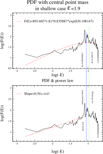
Figure 1: In both panels the data give the PDF of the simulation for a shallow initial density profile ($\epsilon=1.9$) when averaged over the self-similar phase. The simulation was run with a small central point mass ($~{}5\times 10^{-4}$ the total mass of the halo) that substantially reduces the noise in the core without affecting the global behaviour. The upper panel shows an attempt to fit a power law times an exponential, while the lower panel fits a power law up to the point where the curvature may not be ignored.

In figure (2) the density profile established in the dark matter core near the end of the self-similar phase is shown. We see principally that the theoretical attractor profile of $r^{-2}$ is quite convincingly established over an intermediate range of scales that extends to the interior of the smoothing scale. We take this to be confirmation of the idea that the main relaxation of the core occurs near the boundary turning point since in this case more than the initial conditions are required to achieve the attractor profile as found.

Figure 2: Density Profile established near the end of the Self-Similar phase for an initially slightly flat perturbation. The smoothing scale is shown by a vertical line, but the straight line fit with slope $-2$ extends to the interior of this scale. The particles in the outer mixing zone of the halo have been neglected. The NFW profile provides a poor fit in this purely radial case.

The profile steepens at the outside due partly to the absence of particles ( the ‘Keplerian effect’ see e.g. [Henriksen and Widrow 1999]) and partly perhaps due to the fine grained entropy effect (the outer parts of the core retain the pure phase mixing ) suggested at the end of the section on radial orbits. The flattening at small radii here is largely due to the dominance of the point mass potential. For this purely radial model with a central point mass the NFW profile provides a poor fit as shown.

In figures (3) and (4) the same information as above for a ‘slightly steep’ case is presented (the expected slope of $2\alpha/\delta=2.03$ by equation (90).

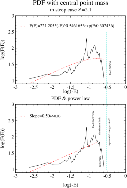
Figure 3: In both panels the data give the PDF of the simulation for a steep initial density profile ($\epsilon=2.1$) when averaged over the self-similar phase. The simulation was run with a small central point mass ($~{}5\times 10^{-4}$ the total mass of the halo) that substantially reduces the noise in the core without affecting the global behaviour. The upper panel shows an attempt to fit a power law times an exponential, while the lower panel fits a power law up to the point where the curvature may not be ignored.

The PDF is again shown fitted by a negative temperature exponential times a power and by a pure power law. The power law fit yields $0.50\pm.03$ when it is taken from the outer core regions to the maximum of the exponential curve, some one and one-half decades. However it is a poor detailed fit to the data here and must be considered a weaker result than is the shallow case. The steep cut off at high negative energies probably comes in this case from the finite numerical resolution of the central regions (where now the most negative energy particles initially, originate), but once again there is a hint of a gaussian just before this cut-off.

Figure (4) shows that the steep simulation has reproduced the expected density profile in the intermediate scales rather accurately, and that the profile continues well inside the smoothing length as anticipated. There is also the outer Keplerian steepening and an inner flattening due to the potential of the central point mass. Once again no globally good fit with the NFW profile is possible.

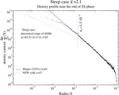
Figure 4: Density Profile established near the end of the Self-Similar phase for an initially slightly steep perturbation. The smoothing scale is shown by a vertical line, but the straight line fit with slope $-2.03$ extends to the interior of this scale. The particles in the outer mixing zone of the halo have been neglected. The NFW profile can provide a good fit to the outer part of the halo but it is far too flat in the inner regions for these purely radial orbits.

We believe that these numerical experiments offer some confirmation of the ideas expressed earlier in this paper and in [Henriksen and Widrow 1999]. In particular the radial PDF is more strongly suggested to be $(-E)^{1/2}$ in the relaxed self-similar region. This cuts off at large negative energies due to a combination of initial conditions and finite mass resolution, but before this occurs, there is slight evidence for a Gaussian form in the central regions as suggested by our coarse graining in section (2).

The density profiles agree with previous work in the self-similar infall phase, but we have reduced the noise in the simulation by the device of including a central point mass of negligible size. The fact that the slopes continue substantially inside the smoothing length suggests that the key behaviour determining the profile occurs in the mixing region near the boundary of the core (and $v=0$) combined with the initial conditions. This also agrees with and supports our coarse graining argument of section (3). It is also clear from these figures that the NFW profile can not provide a global fit to these radial infall models. This then requires an exploration of the effects of angular momentum, which we reserve for the next paper in this series.

6 Conclusions and Summary

Our main interest in this paper has been to test the usefulness of a proposed coarse-graining (actually a progressively finer grained series) technique that uses non-canonical coordinate transformations on the phase space of a dynamical system. This was used in two cases in sections (2) and (3) respectively. The first section concerned itself with the coarse graining of an equilibrium, spherically symmetric system by a stretching transformation on phase space. This allowed us to conclude that near the centre of such a system regularity of the coarse graining expansion imposed some conditions on the coarse-grained $f(v^{2})$. The one which maintained its form to all orders and which gave the same form at all sufficiently small $r$, was a Gaussian. We also checked that the entropy decreased in the higher orders (finer grained) of the expansion without imposing further constraints. The coarse graining expansion led naturally to the small $r$ expansion for the density profile that is familiar from the theory of polytropes.

In the second section we treated the radial self-similar infall model that is of significance for cosmological dark matter halos. The coordinate transformation used for the coarse graining was also the transformation that renders the system stationary. We found that the coarsest grained density profile was already that dictated by the self-similarity class implicit in the initial conditions. Some evidence for this behaviour was found in the numerical simulations of section (5) in that the density profile extended well inside the smoothing length of the simulation. We concluded that the actual relaxation of the system took place near the ‘boundary’ of the core.

The requirement that the self-similarity be stable in these coordinates to all orders of the coarse-graining expansion (ie essentially that the coarse grained and fine grained DF’s be equal) yielded the self-similar DF as $f\propto\delta(j^{2})(|E|)^{1/2}$. This had been previously conjectured in [Henriksen and Widrow 1999], but the present argument is more direct. Moreover from our simulations the evidence presented in support of this result appears stronger than before, although we incorporate a partly analytical estimate of the shell energy here rather than use the much noisier numerical calculation. Had we not done this our evidence would have been weaker than in [Henriksen and Widrow 1999]. We also found that the presence of a point mass at the centre of the system greatly reduced the noise throughout the core in our simulations.

Eventually the DF is cut off in the central regions of the system (large negative energies) due to finite mass resolution and/or initial conditions. There is weak evidence for a Gaussian in velocity (an exponential in energy) before this cut-off, as might be expected from the work of section (2). This is because the central regions of the core resemble a steady state as discussed in [Henriksen and Widrow 1999], due probably to the relaxation time being short compared to the ‘accretion time’ (time to significantly change the mass) in this region.

By expressing the entropy in the scaled variables and requiring the coarse-grained entropy to be positive, we saw that there was an inner limit to the self-similarity for the cosmologically ‘steep’ case. Similarly there was an outer limit to the extent of the cosmologically ‘flat’ case. The limiting case which has an inverse square density profile has an exactly constant entropy in self-similar variables that is always positive. It diverges for an infinite system but it is likely to be the most stable intermediate profile for finite systems.

By requiring the next finer grained entropy contribution to the total entropy to be negative (corresponding to the increased information at this order) we inferred that the initially steep self-similar infall should flatten, primarily at the centre of the system, while the initially flat self-similar infall should steepen, primarily near the exterior. In this way an intermediate attractor behaviour exists in the self-similar infall model. However the behaviour at small radii is sensitive to the presence of point masses while the behaviour at large radii (exterior to most of the mass) tends to be Keplerian ([Henriksen and Widrow 1999]). Thus the global profile is more subtle in the manner of the NFW fit. However these purely radial systems are NOT well fitted by the NFW profile.

We also studied theoretically (but not numerically) the spherically symmetric infall model in the presence of non-zero angular momentum. We showed that the coarse graining expansion can be carried out in just the same way as for radial orbits. The expected density profiles are not changed and flattening is expected in the central regions. The flattening is of a progressive nature and becomes even flatter than $r^{-1}$ of the NFW profile as $r\rightarrow 0$. This is compatible with the expected Gaussian DF in the central regions of the system, although this can only be established definitely by examining higher orders in the expansion. There is an interesting dependence of the expected outer power law and flattening on scale through the index of the initial density perturbation (related to the power spectrum index $n$). This is such as to predict flatter cusps for galaxies than the NFW profile, which in turn is most appropriate on cluster scales or above ($n=1$).

We were able also to constrain the form of the DF in the relaxed state when the coarse grained and fine grained functions are the same as in (83). These relaxed DF’s are steady states as is the radial equivalent. They appear to be consistent with a possible Gaussian DF modulated by a function that allows for inner and outer turning points at a given $j^{2}$. This is presumably due to the somewhat artificial constraint of spherical symmetry, which restricts the relaxation in angular momentum.

We have found that the NFW profile can be produced in such a spherical system with an appropriate distribution of angular momentum (and no central black holes). However the angular momentum has to be correlated with initial radius of a particle in a power law fashion that is consistent with the self-similarity. Once again this may work only in the absence of strong relaxation in angular momentum. We intend to explore this question by coarse graining axially symmetric systems in a subsequent paper.

7 Acknowledgements

RNH acknowledges the support of an operating grant from the canadian Natural Sciences and Research Council. M LeD wishes to acknowledge the financial support of Queen’s University.

References

- [Binney and Tremaine 1987] Binney J., Tremaine S., 1987, Galactic Dynamics, Princeton Univ. Press, Princeton, chapter 4
- [Bertschinger 85] Bertschinger E., 1985, ApJS, 58,39
- [Carter and Henriksen 1991] Carter B., Henriksen R.N., 1991, J. Math. Phys., 32,2580
- [Chandrasekhar 1957] Chandrasekhar S., 1957, Stellar Structure, Dover, 1957, 94
- [DE Blok 01] DE Blok W.J.G., McGaugh Stacy S., Bosma Albert, Rubin Vera C., 2001, astro-ph/0103102v2.
- [Evans and Collett 1997] Evans N.W., Collett J.L., 1997, ApJ, 480, L103
- [Fillmore and Goldreich 1984] Fillmore J.A., Goldreich P., 1984, ApJ, 281,1
- [Fujiwara 1983] Fujiwara T., 1983, PASJ, 35, 547
- [Henriksen and Widrow 1995] Henriksen R.N., Widrow L.M., 1995. MNRAS, 276,679
- [Henriksen 1997] Henriksen R.N., 1997, in Dubrulle B., Graner F., Sornette D., eds. Scale Invariance and Beyond, les Houches Workshop, Springer, Berlin,p63
- [Henriksen and Widrow 1997] Henriksen R.N., Widrow L.M., 1997, Phys.Rev.Lett., 78, 3426
- [Henriksen and Widrow 1999] Henriksen R.N., and Widrow L. M., 1999, Mon.Not.R.Astron.Soc. 302, 321
- [Kravtsov 98] Kravtsov A.V., Klypin A.A., Bullock J.S., Primack J.R., 1998, ApJ, 502,48
- [Kulessa 92] Kulessa A.S., Lynden-Bell D., 1992, MNRAS, 255,105
- [Le Delliou 2001] Le Delliou Morgan, 2001, Ph.D. thesis, Queen’s Univ. at Kingston, Canada
- [Lynden-Bell 1967] Lynden-Bell D., 1967, MNRAS, 136, 101
- [Merritt and Cruz 2001] Merritt David, Cruz Fidel, 2001, astro-ph/0101194v2.
- [Merrit, Tremaine and Johnstone, 1989] Merritt D., Tremaine S., Johnstone D., 1989, MNRAS, 236, 829
- [Moore 98] Moore B., Governato F., Quinn T., Stadel J., Lake G., 1998, ApJ, 499, L5
- [Nakamura 2000] Nakamura Tadas K., 2000, ApJ, 531, 739
- [Navarro,Frenk and White 1996] Navarro J.F.,Frenk C.S., White S.D.M., 1996, ApJ, 462, 563
- [Shu 1978] Shu F., 1978, ApJ, 225,83
- [Shu 1987] Shu F., 1987, ApJ, 316, 502
- [Stil 99] Stil J., Doctoral Thesis, Leiden Observatory, Netherlands.
- [Syer and White 1998] Syer D., White S.D.M., 1998, MNRAS, 293, 337