Observable consequences of cold clouds as dark matter

Abstract

Cold, dense clouds of gas have been proposed as baryonic candidates for the dark matter in Galactic haloes, and have also been invoked in the Galactic disc as an explanation for the excess faint sub-mm sources detected by SCUBA. Even if their dust-to-gas ratio is only a small percentage of that in conventional gas clouds, these dense systems would be opaque to visible radiation. This presents the possibility of detecting them by looking for occultations of background stars. We examine the possibility that the data sets of microlensing experiments searching for massive compact halo objects can also be used to search for occultation signatures by cold clouds. We compute the rate and timescale distribution of stellar transits by clouds in the Galactic disc and halo. We find that, for cloud parameters typically advocated by theoretical models, thousands of transit events should already exist within microlensing survey data sets. We examine the seasonal modulation in the rate caused by the Earth’s orbital motion and find it provides an excellent probe of whether detected clouds are of disc or halo origin.

1 INTRODUCTION

Over the last decade several workers have suggested that the Galaxy may contain a large population of cold ($T\la 10$ K), dense, low-mass clouds of molecular material. Several authors have argued that the mass contained in such clouds could be responsible for keeping galaxies’ rotation curves flat beyond the edges of optical discs. Pfenniger & Combes (1994) argued that the clouds would be an integral part of a fractal interstellar medium and be confined to a thin disc. By contrast, de Paolis et al. (1995), Gerhard & Silk (1996), Draine (1998), and Walker & Wardle (1998) considered the case of cold clouds that are distributed in an approximately spherical halo. De Paolis et al, Draine and Gerhard & Silk argued for clouds of approximately solar mass, while Walker & Wardle pointed out that ionized winds from clouds with masses around a Jupiter mass ($\,M_{\rm J}$) could explain the extreme scattering events that are frequently observed in the light curves of pulsars seen at low Galactic latitudes.

A major issue with these proposals that a significant mass is locked up in very small clouds, is to understand why the clouds do not collapse to form stars or degenerate objects such as brown dwarfs. Sciama (2000) has argued that cosmic-ray heating may be able to balance molecular cooling in a stable way for dust-free clouds, whilst Lawrence (2001) has presented similar arguments that cosmic-ray heating could balance cooling by dust emission in dusty clouds. Clouds that are an integral part of the ISM would be expected to be dusty, and radiate strongly at sub-mm wavelengths. Lawrence (2001) has considered the possibility that a significant fraction of the reddest SCUBA sources could lie in the Galaxy. He concludes that for dusty clouds, masses between $\sim 10\,M_{\rm J}$ and $\sim 10\,{\rm M}_{\sun}$ can be ruled out, and that a population that contributes significantly to the SCUBA counts will make a significant contribution to the mass of the Galaxy only if they have masses $\sim M_{\rm J}$. These objects would have to be confined to the Galactic plane.

The clouds would have temperatures $T\sim 10$ K, and if they were in virial equilibrium, they would be $\sim 20$ AU in diameter and totally opaque at optical wavelengths (and even have an optical depth of order unity at 1 mm). Their number density on the sky has to be comparable to that, $\sim 1000$ deg^-2, of unidentified SCUBA sources, so they would cover a fraction $\sim 10^{-6}$ of the sky. Consequently, at any given time, of order one star in a million should be occulted by one of these clouds. It should be feasible to detect such occultations in the databases that have been produced in searches for microlensing events (for a recent overview of microlensing results see Kerins, 2001, and references therein).

Here we investigate the rate at which stars would be occulted by opaque clouds.We argue in Section 2 that halo and disc clouds are likely to have the characteristics required to produce observable transits. In Section 3 we derive general formulae for the rate and timescale distribution of transit events and in Section 4 we apply them to a specific Galactic model. Currently available microlensing databases refer to a handful of lines of sight. The largest body of data refers to lines of sight in the general direction of the Galactic centre. Other extensive data sets refer to sight lines towards the Magellanic Clouds. Consequently, we concentrate on predictions for these particular directions. We also investigate means by which halo and disc cloud populations could be differentiated.

2 Cloud characteristics and detectability

In order to occult background stars cold clouds must meet certain criteria. Firstly, the clouds must be sufficiently diffuse that they do not appreciably gravitationally lens the starlight. The case of gravitational lensing by gas clouds has been studied previously by Henriksen & Widrow (1995). A necessary condition to avoid the gravitational lensing regime is that the cloud radius $R$ exceeds the Einstein radius, leading to the requirement that

$$R\gg 0.3\,{\rm AU}\;\left(\frac{M}{10^{-3}\,{\rm M}_{\sun}}\right)^{1/2}\left(\frac{D}{10\,{\rm kpc}}\right)^{1/2},$$ (1)

where $M$ is the cloud mass and $D\equiv D_{\rm c}(D_{\rm s}-D_{\rm c})/D_{\rm s}$, with $D_{\rm c}$ ($D_{\rm s}$) the distance between the observer and cloud (source).

The long-term stability of cold ($T\sim 10~{}K$) clouds is an open issue and a serious theoretical problem for the scenario. If opaque clouds can be stabilized against collapse, their size would be of the same order as their virial radius (c.f. Lawrence, 2001)

$$R_{\rm vir}=7\,{\rm AU}\;\left(\frac{M}{10^{-3}\,{\rm M}_{\sun}}\right)\left(\frac{T}{10~{}K}\right)^{-1}.$$ (2)

$R\sim R_{\rm vir}$ would also satisfy the lensing condition in equation (1) provided

$$M\gg 1.6\times 10^{-6}\,{\rm M}_{\sun}\;\left(\frac{T}{10~{}\mbox{K}}\right)^{2}\left(\frac{D}{10\,{\rm kpc}}\right).$$ (3)

This condition is satisfied for almost all plausible clouds since, regardless of their formation mechanism, hydrogenous clouds less massive than $\sim 10^{-7}\,{\rm M}_{\sun}$ evaporate away over a Hubble time (de Rújula, Jetzer & Massó, 1992).

Diffuse clouds will still refract, rather than occult, starlight if they are transparent (Walker & Wardle, 1998; Draine, 1998). How opaque might we expect the clouds to be? The average hydrogen column density through a virialized cloud of is

$$N_{\rm H}=3.3\times 10^{-29}~{}\mbox{m}^{-2}\;\left(\frac{R}{7\,{\rm AU}}\right)^{-1}\left(\frac{T}{10~{}K}\right)^{2}.$$ (4)

Assuming typical dust properties, the visual extinction through a cloud is therefore (e.g. Binney & Merrifield, 1998)

$$A_{V}=1.7\times 10^{4}\,f\;\left(\frac{R}{7\,{\rm AU}}\right)^{-1}\left(\frac{T}{10~{}K}\right)^{2},$$ (5)

where $f$ is the factor by which the cold cloud dust-to-gas ratio exceeds that of typical Galactic molecular clouds. Equation (5) implies that if cold clouds have even remotely the same dust abundance as normal clouds then they easily fulfill the requirement that they be opaque to starlight. In fact, for the clouds not to produce a detectable occultation (which, conservatively, requires $A_{V}<1$) they must have a dust-to-gas ratio at least four orders of magnitude lower than is measured for ordinary gas clouds, i.e. they must be essentially dust free.

We should expect disc clouds to have a similar dust-to-gas ratio as the interstellar medium and therefore be completely opaque. However, equation (5) also implies strong limits on halo cloud properties for them to escape detection by occultation. This can be more clearly seen by considering how halo clouds may have interacted with the interstellar medium over the lifetime $\tau_{\rm gal}$ of the Galaxy. Over this time one would expect a typical halo cloud to have passed through the Galactic disc $N$ times, where

$$N \sim \sigma\tau_{\rm gal}/2r_{\rm c}$$ (6)

$$\sim 160\left(\frac{\sigma}{160\,{\rm km}~{}{\rm s}^{-1}}\right)\left(\frac{\tau_{\rm gal}}{10~{}\mbox{Gyr}}\right)\left(\frac{r_{\rm c}}{5\,{\rm kpc}}\right)^{-1},$$

with $r_{\rm c}$ and $\sigma$ the halo core radius and velocity dispersion. Neglecting accretion the mass swept up by these clouds on each passage through an exponential disc is

$$M_{\rm sweep} \sim 2\pi\varepsilon R^{2}\rho H=4\times 10^{-8}~{}\,{\rm M}_{\sun}\,\varepsilon\left(\frac{R}{7~{}\mbox{AU}}\right)^{2}$$ (7)

$$\hskip 48.36958pt\times\left(\frac{\rho}{0.03\,{\rm M}_{\sun}\mbox{pc}^{-3}}\right)\left(\frac{H}{200~{}\mbox{pc}}\right),$$

where $\rho$ is the typical density of gas in the plane of the disc, $H$ the disc scale height and $\varepsilon$ the efficiency with which the clouds retain swept up gas. Adopting the parameter values in equations (6) and (7) implies that the present mass fraction of swept-up disc gas in a typical halo cloud is $NM_{\rm sweep}/M\sim 0.007\,\varepsilon$ for a $10^{-3}\,{\rm M}_{\sun}$ cloud.This, together with equation (5), indicates that provided $\varepsilon>0.008f^{-1}$ the cloud dust-to-gas ratio should be large enough to produce at least a one magnitude diminution in the light from background stars.

Lastly, we need to know how easily the flux change from transit events can be detected. An important consideration is source resolvability. For Galactic microlensing experiments it is often the case that more than one star occupies the seeing disc, leading to a detection bias referred to as blending (Alard, 1997). The situation is more extreme for experiments looking towards M31 where there are many stars per detector pixel. Transit events could escape detection by these surveys if the occulted star lies so close to other stars that the effect of its occultation is masked by light from other stars. Quantitatively, if a fraction $f_{*}$ of the flux in the seeing disc comes from the target star, the flux at minimum will be a fraction $(1-f_{*})+f_{*}10^{-0.4A_{V}}$ of the flux prior to occultation. Equating this fraction to $10^{-0.4\Delta M_{T}}$, where $\Delta M_{T}$ is the smallest magnitude change a survey can measure, we find that the event will be detected only if

$$f_{*}\ga\frac{1-10^{-0.4\Delta M_{\rm T}}}{1-10^{-0.4A_{V}}}$$ (8)

For completely opaque clouds (large $A_{V}$) the requirement is simply $f_{*}\ga\Delta M_{\rm T}$ for $\Delta M_{\rm T}\ll 1$. In the context of gravitational microlensing searches, experiments to detect microlensing events in our Galaxy typically adopt the very conservative value $\Delta M_{\rm T}\sim 0.3$ as a means of excluding variable stars. The M31 surveys typically use a much lower threshold $\Delta M_{\rm T}\sim 0.02$. If similar thresholds are adopted for the detection of transit events then they should be detectable within our Galaxy provided blending effects are not too severe. It may even be possible to detect transit events towards M31 provided the occulted stars ordinarily contribute upwards of $2\%$ of the flux in a seeing disc.

3 TRANSIT RATE AND TIMESCALE DISTRIBUTION

From here onwards we assume that the cold clouds are opaque and exceed their Einstein radius, so that they give rise to observable occultation events. We calculate the rate at which occultations of a given duration should be observed at any season of the year and along any line of sight. Similar calculations of microlensing rates are described by Griest (1991) and Kiraga & Paczyński (1994).

Let there be $n({\bf v}){\rm d}^{2}{\bf v}$ spherical clouds of radius $R$ per unit volume and with velocities in the plane of the sky in ${\rm d}^{2}{\bf v}$. Then in a sheet of thickness ${\rm d}D_{\rm c}$ that extends perpendicular to the line of sight, the rate at which clouds pass a given background star with impact parameters in the range $(b,b+{\rm d}b)$ is

$${\rm d}^{4}\Gamma=n({\bf v}){\rm d}^{2}{\bf v}\,{\rm d}D_{\rm c}\,2v_{\perp}{\rm d}b,$$ (9)

where $v_{\perp}=|{\bf v}|$. In an obvious notation we have ${\rm d}^{2}{\bf v}=v_{\perp}{\rm d}v_{\perp}{\rm d}\theta$, so

$${\rm d}^{4}\Gamma=2n({\bf v})v_{\perp}^{2}{\rm d}v_{\perp}\,{\rm d}\theta\,{\rm d}D_{\rm c}\,{\rm d}b.$$ (10)

An impact with $b<R$ causes an occultation of duration

$$t=2\sqrt{R^{2}-b^{2}}/v_{\perp},$$ (11)

so we may obtain the distribution over durations by eliminating $b$ in favour of $t$. One finds

$${{\rm d}^{4}\Gamma\over{\rm d}D_{\rm c}{\rm d}t}={n({\bf v})v_{\perp}^{3}{\rm d}v_{\perp}\,{\rm d}\theta\,\over\sqrt{(2R/v_{\perp}t)^{2}-1}}$$ (12)

This equation gives the occultation rate of a single source star. To get the rate that can be measured observationally, we have to average it over all detectable source stars (c.f. Kiraga & Paczyński, 1994). If the probability that a source star at distance $D_{\rm s}$ has its velocity on the sky in ${\rm d}^{2}{\bf v_{\rm s}}$ is $p({\bf v_{\rm s}}){\rm d}^{2}{\bf v_{\rm s}}$, then the required average of equation (12) is

$${{\rm d}^{2}\Gamma\over{\rm d}D_{\rm c}{\rm d}t}=\int{\rm d}^{2}{\bf v_{\rm s}}\,p({\bf v_{\rm s}})\int_{0}^{2R/t}\hskip-15.0pt\frac{{\rm d}v_{\perp}\,v_{\perp}^{3}}{\sqrt{(2R/v_{\perp}t)^{2}-1}}\int{\rm d}\theta\,n({\bf v}).$$ (13)

$v_{\perp}$ is the magnitude of the cloud’s transverse velocity with respect to its local point on the line of sight from the source to the Sun; consequently it is a function of ${\bf v_{\rm s}}$. The argument ${\bf v}$ of the velocity distribution $n({\bf v})$ must relate to a fixed frame. In the frame in which the Earth is at rest

$$v_{\perp}=\left|{\bf v}-{D_{\rm c}\over D_{\rm s}}{\bf v_{\rm s}}\right|,$$ (14)

where $D_{s}$ is the distance to the source star, so, for fixed $v_{\perp}$, ${\bf v}$ is a function of ${\bf v}_{s}$ and to make further progress analytically, it is necessary to assume that both ${\bf v}$ and ${\bf v_{\rm s}}$ have Gaussian distributions. Since we are working in the Earth’s rest frame, these Gaussians will be centred on non-zero velocities $\overline{{\bf v}}$ and $\overline{{\bf v}}_{s}$, respectively. Consequently we have

$$p({\bf v_{\rm s}})n({\bf v})={n_{c}\over(2\pi\sigma_{s}\sigma)^{2}}\exp\left[-{({\bf v_{\rm s}}-\overline{{\bf v}}_{\rm s})^{2}\over 2\sigma_{s}^{2}}-{({\bf v}-\overline{{\bf v}})^{2}\over 2\sigma^{2}}\right],$$ (15)

where $n_{c}$ is the volume density of clouds. Now $\theta$ is the direction of ${\bf v}-(D_{\rm c}/D_{\rm s}){\bf v_{\rm s}}$, so with (14) we have

$$({\bf v}-\overline{{\bf v}})^{2} = \left|{\bf v}-{D_{\rm c}\over D_{\rm s}}{\bf v_{\rm s}}+{D_{\rm c}\over D_{\rm s}}{\bf v_{\rm s}}-\overline{{\bf v}}\right|^{2}$$ (16)

$$= v_{\perp}^{2}+2v_{\perp}v_{\rm s}\cos\theta+v_{\rm s}^{2},$$

where

$$v_{\rm s}\equiv\left|{D_{\rm c}\over D_{\rm s}}{\bf v_{\rm s}}-\overline{{\bf v}}\right|.$$ (17)

When we insert (16) into $n({\bf v})$ and integrate over $\theta$ we find

$$\int{\rm d}\theta\,n({\bf v})={n_{c}\over\sigma^{2}}\exp\left[-{v_{\perp}^{2}+v_{\rm s}^{2}\over 2\sigma^{2}}\right]I_{0}\left({v_{\perp}v_{\rm s}\over\sigma^{2}}\right),$$ (18)

where $I_{0}$ is the usual modified Bessel function. Inserting this result in (13) we find

$${{\rm d}^{2}\Gamma\over{\rm d}D_{\rm c}{\rm d}t} = {n_{\rm c}\over 2\pi\sigma_{s}^{2}\sigma^{2}}\int_{0}^{2R/t}\hskip-14.22636pt{v_{\perp}^{3}\,{\rm d}v_{\perp}\over\sqrt{(2R/v_{\perp}t)^{2}-1}}$$ (19)

$$\hskip-28.45274pt\times\int{\rm d}^{2}{\bf v_{\rm s}}\exp\left[-{({\bf v_{\rm s}}-\overline{{\bf v}}_{\rm s})^{2}\over 2\sigma_{s}^{2}}-{v_{\perp}^{2}+v_{\rm s}^{2}\over 2\sigma^{2}}\right]I_{0}\left({v_{\perp}v_{\rm s}\over\sigma^{2}}\right).$$

This result simplifies significantly if the sources have negligible random motions (i.e. $\sigma_{s}D_{\rm c}/D_{\rm s}\ll\sigma$). In this case we can approximate the Gaussian distribution over ${\bf v_{\rm s}}$ by $\delta^{2}({\bf v_{\rm s}}-\overline{{\bf v}}_{\rm s})$, giving

$${{\rm d}^{2}\Gamma\over{\rm d}D_{\rm c}{\rm d}t} \simeq {n_{\rm c}\over\sigma^{2}}\int_{0}^{2R/t}\hskip-14.22636pt{{\rm d}v_{\perp}\,v_{\perp}^{3}\over\sqrt{(2R/v_{\perp}t)^{2}-1}}$$ (20)

$$\quad\quad\quad\quad\quad\times\exp\left[-{v_{\perp}^{2}+v_{\rm s}^{2}\over 2\sigma^{2}}\right]I_{0}\left({v_{\perp}v_{\rm s}\over\sigma^{2}}\right).$$

with $\overline{{\bf v}}_{\rm s}$ replacing ${\bf v_{\rm s}}$ in (17). The rate of occultations integrated over all durations$\int{\rm d}t\,{\rm d}^{2}\Gamma/{\rm d}D_{\rm c}{\rm d}t$ is readily obtained from either (19) or (20):

$${{\rm d}\Gamma\over{\rm d}D_{\rm c}} = {n_{\rm c}R\over\pi\sigma_{s}^{2}\sigma^{2}}\int{\rm d}v_{\perp}\,v_{\perp}^{2}\int{\rm d}^{2}{\bf v_{\rm s}}$$

$$\quad\times\exp\left[-{({\bf v_{\rm s}}-\overline{{\bf v}}_{\rm s})^{2}\over 2\sigma_{s}^{2}}-{v_{\perp}^{2}+v_{\rm s}^{2}\over 2\sigma^{2}}\right]I_{0}\left({v_{\perp}v_{\rm s}\over\sigma^{2}}\right)$$

$$\simeq {2n_{\rm c}R\over\sigma^{2}}\int{\rm d}v_{\perp}\,v_{\perp}^{2}\exp\left[-{v_{\perp}^{2}+v_{\rm s}^{2}\over 2\sigma^{2}}\right]I_{0}\left({v_{\perp}v_{\rm s}\over\sigma^{2}}\right).$$

Since the central velocities $\overline{{\bf v}}_{\rm s}$ and $\overline{\bf v}$ are relative to the Earth, equations (19) to (3) yield occultation rates that depend on observing season.

From equation (3) $\Gamma\propto R/M$ (because $n_{\rm c}\propto\rho/M$), so for virialised clouds equation (2) indicates that the transit rate is controlled simply by the cloud temperature $T$, i.e. $\Gamma\propto T^{-1}$, independent of the scale size of the cloud. However, for fixed dimensionless impact parameter $b/R$ the transit time $t\propto R$ from equation (11) so ${\rm d}\Gamma/{\rm d}t\propto R^{-1}T^{-1}$ when integrated over all impact parameters $0\leq b/R\leq 1$.

In some applications the sources are widely distributed in distance $D_{\rm s}$. In this case we follow Kiraga & Paczyński (1994) in evaluating weighted averages over $D_{\rm s}$ of the rates (19) to (3), with the weight factor taken to be $n_{\rm s}D_{\rm s}^{2+2\beta}$. Here $n_{\rm s}$ is the source volume number density and $\beta$ parameterizes the effects of the luminosity function upon the distance distribution of sources. In our calculations we adopt $\beta=-2$ for $D_{\rm s}>100\,$pc and $\beta=-1$ at smaller distances.

4 MODEL PREDICTIONS

We explore two locations for potential cloud populations, the Galactic disc and halo, and we compute the rate of occultations for lines of sight to three targets: the Large Magellanic Cloud (LMC) at Galactic coordinates $(l,b)=(280\degr,-33\degr)$, the Small Magellanic Cloud (SMC) at $(l,b)=(303\degr,-44\degr)$ and Baade’s Window towards the Galactic Centre (GC) at $(l,b)=(1\degr,-4\degr)$. These are all regions which have been intensively monitored by several experiments looking for microlensing events. As discussed in Section 2, a fourth possibility is the Andromeda Galaxy (M31), though in that case the formulae of the previous Section must be modified to take account of the fact that the sources in M31 are mostly unresolved. We therefore confine our attention in the remainder of this paper to the GC, LMC and SMC only. The LMC and SMC source stars are assumed to lie at fixed distances of $50\,{\rm kpc}$ and $60\,{\rm kpc}$, respectively, whilst background sources towards Baade’s Window are assumed to be distributed throughout the Galactic disc and bar.

Since we are not concerned with the precise details of the halo structure, it is sufficient for our purposes to model the distribution of halo clouds as a simple softened isothermal sphere with a core radius of $5\,{\rm kpc}$ and a local density of $0.01\,{\rm M}_{\sun}\mbox{pc}^{-3}$. The halo velocity distribution is taken to be Gaussian with $\sigma=156\,{\rm km}~{}{\rm s}^{-1}$. For both clouds and sources in the Galactic disc we model their density distribution as a sech-squared profile with a scale length of $2.5\,{\rm kpc}$ and scale height of 190 pc. We assume the clouds contribute up to a third of the disc density and so have a local density of $0.03\,{\rm M}_{\sun}\mbox{pc}^{-3}$. Strong local kinematical and dynamical constraints rule out the existence of a more significant population (Crézé et al., 1998). We adopt a velocity dispersion of $\sigma=25\,{\rm km}~{}{\rm s}^{-1}$ and a rotation speed $v_{\rm rot}=220\,{\rm km}~{}{\rm s}^{-1}$ for both disc clouds and sources, independent of radius.

For calculations towards the LMC and SMC we neglect random stellar motions in the clouds themselves though we do include the bulk motion of the Clouds $(u,v,w)=(60,-155,146)\,{\rm km}~{}{\rm s}^{-1}$ (Jones, Klemola & Lin, 1994), where the $(u,v,w)$ coordinate system is centred on the Sun and the velocity components point, respectively, towards the Galactic Centre, the direction of rotation, and the North Galactic Pole. Equations (20) and (3) are therefore sufficient to compute the halo cloud timescale distribution and rate towards these targets. For bulge sources we adopt the bar model of Bissantz et al. (1997) with exponential scale length $a_{\rm m}=3.82\,{\rm kpc}$, power-law scale length $a_{0}=100$ pc, axis ratios $\eta=\zeta=0.3$ and bar angle $\phi_{0}=25\degr$. We assume a bar pattern speed of $70\,{\rm km}~{}{\rm s}^{-1}\,{\rm kpc}^{-1}$ and a velocity dispersion $\sigma=100\,{\rm km}~{}{\rm s}^{-1}$. Whilst our disc model is simpler than the double-exponential profile of Bissantz et al. (1997) its scale length is the same and the chosen scale height corresponds to the weighted mean of the scale heights in their model. Our overall disc-bulge mass normalization is therefore in good agreement.

The motion of the observer is modeled as the sum of three distinct components: the motion of the LSR $(u,v,w)=(0,v_{\rm rot},0)\,{\rm km}~{}{\rm s}^{-1}$; the Sun’s motion in the direction of the Solar Apex $(u,v,w)=(10,5.2,7.2)\,{\rm km}~{}{\rm s}^{-1}$ (Binney & Merrifield, 1998); and the motion of the Earth around the Sun, where for simplicity we adopt a circular orbit with $v_{\oplus}=30\,{\rm km}~{}{\rm s}^{-1}$.

4.1 Rate and timescale distribution

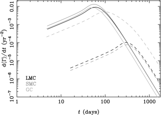
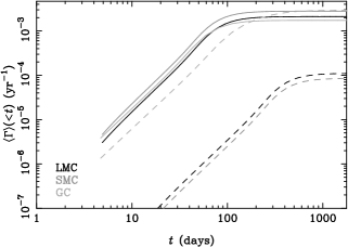
Figure 1: Seasonally-averaged differential (top) and cumulative (bottom) cloud transit timescale distributions for halo clouds, (solid lines) and disc clouds (dashed lines). The distributions are shown for three lines of sight: LMC (black); SMC (dark grey); GC (light grey). The figures assume the clouds have a radius $R=7$ AU and virial temperature $T=10~{}\mbox{K}$. The scaling for other values is ${\rm d}\Gamma/{\rm d}t\propto R^{-1}T^{-1}$ and $t\propto R$.

Fig. 1 shows the predicted distributions of occultation time for both halo and disc clouds towards the LMC, SMC and GC. The distributions are seasonal averages of the timescale distribution. We have adopted a radius $R=7$ AU and virial temperature $T=10$ K for both cloud populations, corresponding to a cloud mass of $M=10^{-3}\,{\rm M}_{\sun}$ from equation (2). The top panel of Fig. 1 shows the differential distribution, whilst the lower panel gives the cumulative rate. For these parameters we see that the halo cloud distributions (solid lines) are peaked at shorter durations than for disc clouds (dashed lines), with the peak occurring around 60 days for all three target directions. For disc clouds the peak occurs at around 100 days in the direction of the GC or around 300 days towards the LMC and SMC.

For fixed cloud temperature the most detectable signals comes from disc clouds observed towards the GC and halo clouds towards the SMC, both with total rates of $\sim 3000$ events/yr per million stars. Halo clouds towards the SMC have the largest rate for transit durations below 500 days. Halo clouds observed towards the LMC and GC have smaller, but comparable, rates. These large rates in comparison with microlensing is due to the size of the clouds. For $10^{-3}\,{\rm M}_{\sun}$ clouds their virial radius is 1.5–2 orders of magnitude larger than the typical Einstein radius of compact objects of the same mass, so the rate is correspondingly higher. Both the timescales and the expected rate are easily within range of current microlensing experiments. Towards the LMC and SMC the disc cloud transit rate is lower by more than an order of magnitude at $\sim 100$ events/yr per million stars. Even when detection efficiencies have been taken into account, microlensing data sets should contain hundreds or even thousands of transit events, so it is clear that much of the parameter space for both halo and disc cloud populations can be probed.

4.2 Discriminating between disc and halo clouds

Can we discriminate between halo and disc cloud populations? From Fig. 1 it is apparent that a rate of $\ga 1000$ events/yr per million sources towards the LMC and SMC would argue strongly for a halo origin. Another obvious diagnostic is the transit duration. Fig. 1 indicates that we should expect few halo cloud events with transit durations above 100 days, whilst more than three-quarters of the rate of disc clouds towards the GC comes from events with durations above 100 days. Of course larger halo clouds can produce longer transits so this is not a robust test.

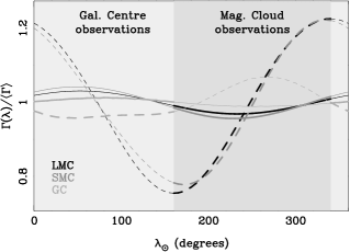
Figure 2: Seasonal modulation of the occultation rate. Displayed as a function of Solar Ecliptic longitude, $\lambda_{\sun}$, is the instantaneous rate, $\Gamma$, expressed as a ratio of the seasonally-averaged rate, $\langle\Gamma\rangle$. Line coding is as for Fig. 1. The approximate observing season for the LMC and SMC is shown by the dark grey shaded region whilst the GC monitoring period is shown in light grey. The modulation curves are shown as thick lines during the relevant observing season and as thin lines otherwise.

A potentially cleaner test is the seasonal modulation in the observed rate due the Earth’s motion around the Sun. The modulation is most pronounced for nearby clouds, which will typically be disc clouds. Fig. 2 shows the modulation in the instantaneous transit rate $\Gamma$, as a ratio of the seasonally-averaged rate $\langle\Gamma\rangle$. The modulation is plotted as a function of Solar Ecliptic Longitude, $\lambda_{\sun}$, where $\lambda_{\sun}=0$ at the Vernal Equinox which occurs around March 21st. The dark grey region of the figure, spanning from September to March, indicates the six-month period when microlensing experiments monitor the Magellanic Clouds. For the rest of the year the GC is observed, as shown by the light grey region. Consequently, only half of the modulation period is accessible for any of the targets, so the modulation curves are shown as bold lines whilst the relevant target is observed and as thin lines when not.

The largest modulation occurs for disc clouds observed towards the LMC and SMC. During the LMC/SMC observing season the rate swings from 0.8 to 1.2 times the seasonal average, a modulation of $20\%$. Assuming $100\%$ detection efficiency, a $20\%$ modulation could be detected at the $3\,\sigma$ level after four seasons of data for a million sources. Current experiments are monitoring closer to $10^{7}$ sources towards the LMC, though their detection efficiency to transits will be somewhat less than $100\%$. It’s nonetheless clear that this modulation should be detectable already. Halo clouds show only a small (few percent) variation in their rate towards the LMC and SMC, however their transit rate is much larger than for disc clouds. A sample upwards of 30000 transit events is required to detect a modulation of $2\%$ at greater than $3\,\sigma$ significance. Experiments monitoring $10^{7}$ sources would amass such a sample within four years, so even this small modulation should be evident within existing data sets. Towards the GC the modulation of the disc and halo cloud rate is similarly small but the rate is comparably large, so again the modulation should be apparent. In the case of halo clouds, observations towards the GC should show a maximum rate during mid-season, whilst disc clouds should exhibit a minimum. The modulation signal should therefore provide a good test for the origin of detected events.

5 DISCUSSION

Cold opaque clouds can be detected by searching data sets already compiled by groups searching for gravitational microlensing events. Rather than the flux excess that is the signature of microlensing, cold cloud events are characterized by a transient dimming of background sources. Like microlensing, this signal should be non-periodic and one should expect events to involve a representative population of background source stars. In selecting microlensing events one problem is to reject variable stars which may mimic a microlensing signal. The equivalent “background” for cloud transit events is potentially much smaller since there are fewer classes of objects which involve a significant dimming of flux. One such class, eclipsing binaries, is unlikely to present much of a problem. For short-period systems their true nature would be evident over the lifetime of the surveys. Binary systems with longer periods for which only one flux dropout is detected, should statistically comprise more massive stars, so we should expect the source stars of these “events” to be unrepresentative of the target stellar population as a whole, contrary to expectation for true cloud transit events. It is also likely that the light-curve of cloud transit events would have a form which generally would be inconsistent with that of eclipsing binaries.

The previous section demonstrates that the transit rate and timescales of cold clouds in the disc and halo is well within the range of detectability if they constitute a significant population and are of a Jupiter mass scale. Whilst the total rate depends only on the temperature of the clouds, virialized clouds more massive than $\sim 0.05\,{\rm M}_{\sun}$ would have transit durations exceeding the present baseline of microlensing experiments.

The seasonal modulation of the rate provides a promising method to distinguish whether the clouds are in the disc or the halo. There are already strong arguments from the consideration of sub-mm sources (Lawrence, 2001) that opaque cold clouds do not contribute much to the halo dark matter budget, though these arguments are sensitive to the precise dust properties of the clouds. Existing microlensing data sets represent a significant corpus of data which can provide an independent line of approach. Though originally conceived as a probe only of compact objects, microlensing surveys may also turn out to be one the most sensitive probes of diffuse cold clouds.

References

- Alard (1997) Alard, C., 1997, A&A, 321, 424
- Alcock et al. (2000) Alcock C., et al. 2000, ApJ, 542, 281
- Binney & Merrifield (1998) Binney, J., Merrifield, M., 1998, Galactic Astronomy, Princeton University Press (Princeton, New Jersey)
- Bissantz et al. (1997) Bissantz, N., Englemaier, P, Binney, J., Gerhard, O., 1997, MNRAS, 289, 651
- Crézé et al. (1998) Crézé, M., Chereul, E., Bienaymé, O., Pichon, C., 1998, A&A, 329, 920
- de Paolis et al. (1995) de Paolis, F., Ingrosso, G., Jetzer, P., Qadir, A., Roncadelli, M., 1995, A&A, 299, 647
- de Rújula, Jetzer & Massó (1991) de Rújula, A., Jetzer, P., Massó, E., 1991, MNRAS, 250, 348
- de Rújula, Jetzer & Massó (1992) de Rújula, A., Jetzer, P., Massó, E., 1992, A&A, 254, 99
- Draine (1998) Draine, B., 1998, ApJ, 509, L41
- Gerhard & Silk (1996) Gerhard, O., Silk, J., 1996, ApJ, 472, 34
- Griest (1991) Griest, K., 1991, ApJ, 366, 412
- Henriksen & Widrow (1995) Henriksen, R., Widrow, L., 1995, ApJ, 441, 70
- Jones, Klemola & Lin (1994) Jones, B.F. Klemola, A.R., Lin, D.N.C., 1994, AJ, 107, 1333
- Kerins (2001) Kerins, E.J., 2001, in Cosmological physics with gravitational lensing, XXXVth Rencontres de Moriond, eds. Tran Thanh Van, Mellier, Moniez, EDP Sciences, p43
- Kiraga & Paczyński (1994) Kiraga, M., Paczyński, B., 1994, ApJ, 430, L101
- Lawrence (2001) Lawrence, A., 2001, MNRAS, 323, 147
- Paczyński (1986) Paczyński, B., 1986, ApJ, 304, 1
- Pfenniger & Combes (1994) Pfenniger, D., Combes, F., 1994, A&A, 285, 94
- Sciama (2000) Sciama, D., 2000, MNRAS, 312, 33
- Walker & Wardle (1998) Walker, M., Wardle, M., 1998, ApJ, 498, L125