THERMAL INSTABILITY IN A COOLING AND EXPANDING MEDIUM INCLUDING SELF-GRAVITY AND CONDUCTION

Abstract

A systematic study of the linear thermal stability of a medium subject to cooling, self–gravity and thermal conduction is carried out for the case when the unperturbed state is subject to global cooling and expansion. A general, recursive WKB solution for the perturbation problem is obtained which can be applied to a large variety of situations in which there is a separation of time-scales for the different physical processes. Solutions are explicitly given and discussed for the case when sound propagation and/or self–gravity are the fastest processes, with cooling, expansion and thermal conduction operating on slower time-scales. A brief discussion is also added for the solutions in the cases in which cooling or conduction operate on the fastest time-scale. The general WKB solution obtained in this paper permits solving the problem of the effect of thermal conduction and self-gravity on the thermal stability of a globally cooling and expanding medium. As a result of the analysis, the critical wavelength (often called Field length) above which cooling makes the perturbations unstable against the action of thermal conduction is generalized to the case of an unperturbed background with net cooling. As an astrophysical application, the generalized Field length is calculated for a hot ($10^{4}-10^{8}$ K), optically thin medium (as pertains, for instance, for the hot interstellar medium of SNRs or superbubbles) using a realistic cooling function and including a weak magnetic field. The stability domains are compared with the predictions made on the basis of models for which the background is in thermal equilibrium. The instability domain of the sound waves, in particular, is seen to be much larger in the case with net global cooling.

1 INTRODUCTION

Thermal instability often appears in astrophysical media which are undergoing a global process of cooling, expansion or contraction. A non-exhaustive list of examples includes: thermal instability in a cooling flow in a galaxy cluster (Mathews & Bregman, 1978; Balbus & Soker, 1989; Balbus, 1991), in a stellar wind (Balbus & Soker, 1989), or in the hot ISM (Begelman & McKee, 1990), and structure formation in a collapsing protogalaxy (Fall & Rees, 1985). In all those cases, the unperturbed state is not one of thermal or dynamical equilibrium, so that the stability and the time evolution of the perturbations cannot be studied by means of a classical normal–mode Fourier analysis in time. The situation is complicated by other physical processes which can be important for the unperturbed state or for the perturbation itself, like self-gravity, thermal conduction, and magnetic induction and diffusion. The stability criteria and the evolution of the perturbations directly depend on the relative time-scale of the latter processes with respect to each other and to the time-scales of cooling and expansion of the background in which they are developing.

The astrophysical literature abounds in examples of thermal stability analyses and their application to specific problems, as in Parker (1953), Weymann (1960), Field (1965), Goldsmith (1970), Defouw (1970), Heyvaerts (1974), Mathews & Bregman (1978), Flannery & Press (1979), Balbus (1986, 1991), Malagoli, Rosner & Bodo (1987), Balbus & Soker (1989), Begelman & McKee (1990), Loewenstein (1990), Chun & Rosner (1993), Burkert & Lin (2000). A milestone was the paper by Field (1965). He considered a non-expanding homogeneous medium in thermal equilibrium (i.e., with cooling exactly compensating heating), including thermal conduction and magnetic fields. The small–perturbation problem is then amenable to a normal-mode Fourier analysis in space and time. Additionally to magnetosonic waves, which can be strongly modified by the thermal processes, he found a non-oscillatory mode (called condensation mode) which may have an isobaric or isochoric character depending on the amount of cooling or conduction possible during one crossing time of a magnetosonic wave across the perturbation. Conduction becomes important at small spatial scales and, in general, has a strongly stabilizing effect. Another important step forward was taken by Mathews & Bregman (1978) and Balbus (1986), who considered a time–dependent unperturbed medium. By using the entropy equation, they obtained stability criteria for the condensation mode in a medium with global cooling, not taking into account conduction, self-gravity or any background stratification. Balbus (1986), in particular, carried out a WKB analysis in space for radial perturbations in an expanding or contracting medium with spherical symmetry. Balbus & Soker (1989) relaxed the condition of homogeneous background and obtained solutions for a stratified medium. Balbus (1991) also included a background magnetic field.

The topic of thermal instability in astrophysical media seems to have been gathering momentum in the past several years. In spite of the foregoing, there is to date no systematic study of the stability of a magnetized medium subject to cooling, self-gravity and thermal conduction when the unperturbed state itself is undergoing expansion and cooling. The purpose of the present paper is to carry out such a study using, wherever possible, a WKB expansion in time. The treatment introduced here permits recovering many results of the previous literature in a unified manner and allows obtaining new ones. The non-magnetic and non-stratified case is considered in the present paper, which deals with the problem of a uniform (but time-dependent) background. However, the results of this paper can also be applied locally to a weakly non-homogeneous background (see sect. 2.5). Several characteristic time-scales have to be considered, to wit, those associated with the background expansion, self-gravity, cooling, sound-wave propagation and conduction. When background cooling and expansion are not the fastest processes in the system, a WKB analysis in time can be carried out. General WKB solutions up to arbitrary order are then obtained and applied to the particular cases when the fastest time-scales are those associated with sound wave propagation, with sound and self-gravity simultaneously, or with conduction.

New results obtained in the present paper are as follows. First, we obtain an expression for the critical length separating stable from unstable domains which generalizes the classical Field length to a system which, in the unperturbed state, is cooling (or otherwise) and expanding or contracting globally. Field (1965) showed the opposite effects of conduction and cooling on the stability of a system in static and thermal equilibrium in the case when the cooling function, $\mathcal{L}$, fulfills $[\partial\mathcal{L}/\partial T]_{p}<0$, and found that below a critical wavelength (the classical Field length) conduction stabilizes the system. Our study permits relaxing the condition of thermal equilibrium in the unperturbed state and including in the latter a global expansion or contraction. We may note that, for lack of a more accurate expression, different authors in the past have tentatively used the value calculated by Field even though their problem involved a medium undergoing global cooling (e.g., David & Bregman, 1989; Pistinner & Shaviv, 1995). In section 5, we calculate the generalized Field length for a medium undergoing a realistic net cooling, and compare it with the classical Field length of a medium in thermal equilibrium with the same cooling but with a balancing constant heating. The results of the present paper also generalize those of Balbus (1986), who considered a medium undergoing global cooling in the unperturbed state, but ignored thermal conduction.

Second, there is in the literature no simultaneous study of the thermal and gravitational linear stability of a medium undergoing net cooling. The combination of both phenomena is important, for example, for the structure formation in a protogalaxy (Fall & Rees, 1985), where condensations previously formed by thermal instability in a cooling medium become gravitationally unstable. In section 3.2 we calculate how the acoustic-gravity modes of Jeans (1902) are modified through conduction and cooling when the background itself is cooling globally. We also show the existence of a hitherto unknown condensation mode in this case. In all these solutions the perturbations can go through different stability regimes: in a cooling medium the generalized Field length and the Jeans length change with time whereas the wavelength of the perturbation remains constant.

There is an alternative to a WKB expansion when trying to solve the problem tackled in this paper. Burkert & Lin (2000) have used a Taylor expansion in time for the reduced problem when there is no thermal conduction, self-gravity or background expansion. Yet, a Taylor expansion has the large disadvantage of being valid only at times small compared with the characteristic times of evolution of the background. This is in contrast to the WKB approach taken in the present paper, which is valid for arbitrary times as long as the perturbation does not grow beyond the linear regime.

The present paper is organized as follows: in section 2, the equations of the problem are presented and the relevant time-scales introduced both for the background and the perturbations. Section 2.5 contains a discussion of the application of the WKB method to the present problem and provides a general WKB solution to the linear perturbation equations. In section 3, a collection of solutions for intermediate wavelengths is presented. The word intermediate is used in the sense that the wavelength is not small nor large enough for conduction or cooling, respectively, to be the dominant processes in the evolution. The case in which sound propagation is the fastest process is considered in section 3.1 whereas in section 3.2 both self-gravity and sound are the fastest processes. Section 4 is devoted to the large and small wavelength regimes and, in particular, to the cases when cooling or conduction operate on the fastest time-scale. In section 5, the generalized Field length and the instability domain are computed for an optically thin medium at high temperature threaded by a magnetic field without dynamical effects (e.g., the hot ISM). The final section (sect. 6) contains a summary and further discussion of the results of the paper.

2 THE EQUATIONS OF THE PROBLEM AND THEIR WKB SOLUTION

This section discusses the physical processes relevant for the present problem, the governing system of equations, and the method used to solve this system. The equations are given first in general (sec. 2.1) and then specialized for the homogeneous unperturbed medium (sec. 2.2) and for small perturbations to that medium (sec. 2.3). There is a considerable number of different physical processes of importance for the present problem: the corresponding time-scales are listed and explained in section 2.4. A general WKB solution to the linear perturbation system is obtained and discussed in section 2.5.

2.1 Equations

We consider an optically thin polytropic ideal gas. The fluid equations that describe the evolution of the system including thermal conduction and self-gravity are:

$$\frac{\displaystyle d\rho}{\displaystyle dt}+\rho{\bf\nabla\cdot v}=0\;,$$ (1)

$$\rho\frac{\displaystyle d{\bf v}}{\displaystyle dt}+{\bf\nabla}p+\rho{\bf\nabla}\Phi=0\;,$$ (2)

$$\frac{{\cal R}}{\mu(\gamma-1)}\rho\frac{\displaystyle dT}{\displaystyle dt}+p{\bf\nabla\cdot v}+\rho\mathcal{L}-{\bf\nabla\cdot}(\chi{\bf\nabla}T)=0\;,$$ (3)

where $d/dt=\partial/\partial t+{\bf v\cdot\nabla}$ is the Lagrangian time derivative, $\gamma$ is the polytropic index of the ideal gas, $\mu$ is the mean atomic mass per particle, ${\cal R}$ is the universal gas constant, $\mathcal{L}(\rho,T)$ (erg s^-1 gr^-1) is the net cooling function (including heating), $\chi(\rho,T)$ is the thermal conduction coefficient and $\Phi$ is the gravitational potential caused by the mass distribution of the system $\Delta\Phi=4\pi G\rho$, with $G$ the universal constant of gravitation. All other symbols have their usual meaning in hydrodynamics. Equations (1), (2) and (3) are the continuity, momentum and energy equations, respectively. The temperature is related to the other quantities by the ideal gas equation: $p=({\cal R}/\mu)\rho T$. The change of $\mu$ due to recombination or ionization processes is not considered in this paper. This is fully acceptable for high enough temperature ($T>10^{5}$K), in which the medium is almost completely ionized, or in situations at lower temperature when the change in $\mu$ is less important than the contribution of cooling and conduction. The thermal instability of a medium in thermal equilibrium with variable $\mu$ has been considered by Goldsmith (1970) and Defouw (1970). Finally, note that the radiative flux in the diffusion limit (optically thick medium) is identical to the classical thermal conduction flux except for the associated conductivity coefficient (e.g., Mihalas & Mihalas, 1984). Therefore, our treatment also allows for the use of radiative transport in the diffusion limit.

2.2 Background Evolution

As a basis for the small–perturbation analysis, we assume a homogeneous background which is expanding uniformly and cooling (or heating) by radiation, so that the unperturbed quantities only depend on time. The background quantities will be denoted with the subscript $0$. The expansion is given by

$${\bf r}=a(t)\,{\bf x}\;,$$ (4)

where ${\bf r}$ is the Eulerian coordinate, ${\bf x}$ is the Lagrangian coordinate and $a(t)$ is the expansion parameter. Using equation (4), the unperturbed velocity field is given by

$${\bf v}_{0}({\bf r},t)=\frac{\dot{a}}{a}\,{\bf r}\;,$$ (5)

where the dot over a symbol (as in $\dot{a}$) indicates its time derivative.

Equations (1) and (3) reduce for the background to

$$\frac{\displaystyle d\rho_{0}}{\displaystyle dt} = -3\frac{\dot{a}}{a}\rho_{0}\;,$$ (6)

$$\frac{d}{dt}\log{T_{0}} = -(\gamma-1)\left(3\frac{\dot{a}}{a}+\frac{\mu}{{\cal R}}\frac{\mathcal{L}_{0}}{T_{0}}\right)\;,$$ (7)

respectively, where $\mathcal{L}_{0}=\mathcal{L}[\rho_{0}(t),T_{0}(t)]$. The time dependence of $a(t)$ must be specified from equation (2). The latter yields

$$\dot{a}={\rm const}$$ (8)

when self-gravity is negligible and

$$\ddot{a}=-\frac{4}{3}\pi G\rho_{0}a\;$$ (9)

otherwise. Additionally, more general forms for $a(t)$ are allowed for the local application of the perturbative analysis around a Lagrangian fluid element in a non-uniform background, as will be explained at the end of section 2.5.

2.3 Linearized Equations for the Perturbations

To obtain a linearized system of equations for the perturbations we proceed as follows. First, we split each variable into unperturbed and perturbed components, indicating the latter with a subscript $1$, like, e.g.

$$\rho_{1}({\bf r},t) {\buildrel\rm def\over{=}} \rho({\bf r},t)-\rho_{0}(t)\,,$$ (10)

$${\bf v}_{1}({\bf r},t) {\buildrel\rm def\over{=}} {\bf v}({\bf r},t)-{\bf v}_{0}({\bf r},t)\,,$$ (11)

and similarly for pressure and temperature. Eulerian linear perturbations are then taken in equations (1) through (3). Thereafter, the Eulerian divergence operator is applied to the momentum equation and all equations are rewritten in terms of the Lagrangian coordinate ${\bf x}$ defined in equation (4). The resulting linear system has coefficients which depend on $t$ but not on ${\bf x}$. We then carry out a spatial Fourier analysis, with Fourier components proportional to $\exp(i\,{\bf k\cdot x})$, so that ${\bf k}$ is the Lagrangian wave vector:

$${\rho_{1}}_{\bf k}({\bf x},t) = {\rho_{1}}_{\bf k}(t)\,\exp(i\,{\bf k\cdot x})\,,$$ (12)

$${{\bf v}_{1}}_{\bf k}({\bf x},t) = {{\bf v}_{1}}_{\bf k}(t)\,\exp(i\,{\bf k\cdot x})\,,\,$$ (13)

and expressions similar to (12) for all other scalar variables (pressure, temperature, etc). For simplicity, we eliminate the index ${\bf k}$ from the Fourier amplitudes in the following. The perturbed velocity is then split into its components parallel and normal to ${\bf k}$:

$${\bf v}_{1}(t)=v_{1}(t)\frac{{\bf k}}{k}+{{\bf v}_{1}}_{\perp}(t)\,.$$ (14)

Finally, the resulting linear system is simplified by repeated use of the background equations and elementary thermodynamic relations. We obtain:

$$\frac{d}{dt}\left(\frac{\rho_{1}}{\rho_{0}}\right) = -i\tilde{k}\,v_{1}\;,$$ (15)

$$\frac{\displaystyle dv_{1}}{\displaystyle dt} = -\frac{\dot{a}}{a}\,v_{1}-i\frac{\omega_{s}c_{s}}{\gamma}\,\frac{p_{1}}{p_{0}}+i\frac{\displaystyle\omega_{g}^{2}}{\displaystyle\tilde{k}}\,\frac{\rho_{1}}{\rho_{0}}\;,$$ (16)

$$\frac{d}{dt}\left(\frac{p_{1}}{p_{0}}\right) = -i\gamma\tilde{k}\,v_{1}-\left(\Omega_{c\rho}+{\tau_{\chi}}^{-1}\right)\frac{p_{1}}{p_{0}}+\left(\Omega_{cp}+{\tau_{\chi}}^{-1}\right)\frac{\rho_{1}}{\rho_{0}}\;,$$ (17)

with all coefficients of the perturbations being evaluated for the background values. As a result of the linearization, the time derivative $d/dt$ in equations (15) through (17) is now given by $d/dt=\partial/\partial t+{\bf v}_{0}\bf{\cdot\nabla}$, i.e., it is the material derivative as one moves with the unperturbed fluid. The other symbols have the following value:

$$\omega_{s}=\tilde{k}c_{s}\;;\qquad\omega_{g}^{2}=4\pi G\rho_{0}\;;$$ (18)

$${\tau_{\chi}}^{-1}=(\gamma-1)\frac{\mu}{{\cal R}}\frac{\chi_{0}}{\rho_{0}}\tilde{k}^{2}\;;$$ (19)

$$\Omega_{c\rho}=(\gamma-1)\frac{\mu}{{\cal R}}T_{0}\left[\frac{\partial}{\partial T}\left(\frac{\mathcal{L}}{T}\right)\right]_{\rho}\qquad\hbox{and}\qquad\Omega_{cp}=(\gamma-1)\frac{\mu}{{\cal R}}T_{0}\left[\frac{\partial}{\partial T}\left(\frac{\mathcal{L}}{T}\right)\right]_{p}\;,\qquad$$ (20)

where

$$c_{s}=\left(\gamma\frac{\displaystyle p_{0}}{\displaystyle\rho_{0}}\right)^{1/2}\qquad\hbox{and}\qquad\tilde{k}=\frac{\displaystyle k}{\displaystyle a}$$ (21)

are, respectively, the adiabatic background sound speed and the Eulerian wavenumber. The coefficients (18)–(20) provide characteristic times for our problem: their meaning and relevance will be discussed in the next section. One also obtains an independent equation for the perpendicular component of the velocity, viz.:

$$\frac{\displaystyle d}{\displaystyle dt}\nabla\times(a^{2}\,{\bf v}_{1})=0\;,$$ (22)

i.e., the integral of the perturbed velocity along a closed material curve remains constant in time.

The system (15)–(17) is a linear ODE system in $t$ for the vector of unknowns $(\rho_{1}/\rho_{0},\,v_{1},\,p_{1}/p_{0})$. Considering the ratio perturbation/background is the natural choice because the unperturbed quantities depend on time. We will say that there is instability if either $|\rho_{1}/\rho_{0}|$ or $|T_{1}/T_{0}|$ grow with time. The velocity perturbation ${\bf v}_{1}$ is not compared with any unperturbed quantity because there is no single unperturbed velocity which could serve as reference at all length scales: at scales smaller than the Jeans length, the sound velocity should be used whereas one should choose $\sqrt{4\pi G\rho_{0}}/k$ for larger scales.

2.4 Characteristic Timescales

A fundamental timescale in the problem is the period of a sound wave, $\tau_{s}=2\pi/\omega_{s}$, with $\omega_{s}$ defined in equation (18). Other important timescales are as follows:

2.4.1 Timescales Associated with Background Expansion and with Self-Gravity

(a) The characteristic time of background expansion is:

$$\tau_{e}=\frac{a}{|\dot{a}|}\;.$$ (23)

This time is also the time-scale for the adiabatic temperature decrease which follows from the expansion (see eq. [7]) and for the inertial change of the perturbed velocity associated with the background expansion (first term on the right-hand side of eq. [16]).

(b) The characteristic growth time of a perturbation by self-gravity, $\tau_{g}$, is

$$\tau_{g}=\left(4\pi G\rho_{0}\right)^{-1/2}\;,$$ (24)

which coincides with $\omega_{g}^{-1}$, as defined in equation (18). From equation (9), $\tau_{g}$ is also the timescale for the deceleration of the background expansion.

2.4.2 Timescales Associated with Cooling and Conduction

(c) The characteristic timescale of background cooling because of radiation, $\tau_{c}$, is given by (see eq. [7])

$$\tau_{c}=\left|\Omega_{c}\right|^{-1}\quad\hbox{with}\quad\Omega_{c}=(\gamma-1)\frac{\mu}{{\cal R}}\frac{\mathcal{L}_{0}}{T_{0}}\;.$$ (25)

For the growth (or otherwise) of the perturbations, one has to consider not only the cooling function itself at a given value of $T_{0}$ and $\rho_{0}$, but also the differential cooling at neighboring values of temperature and density. The precise expression of this fact is obtained through the perturbed energy equation (eq. [17]) rewritten in the form:

$$\frac{d}{dt}\left(\frac{T_{1}}{T_{0}}\right)=-i(\gamma-1)\tilde{k}\,v_{1}-\left(\Omega_{dc}-\Omega_{c}+{\tau_{\chi}}^{-1}\right)\,\frac{T_{1}}{T_{0}}\;,$$ (26)

with the growth rate due to differential cooling, $\Omega_{dc}$, defined as

$$\Omega_{dc}=(\gamma-1)\frac{\displaystyle\mu}{\displaystyle{\cal R}}\left[\left(\frac{\displaystyle\partial\mathcal{L}}{\displaystyle\partial\rho}\right)_{T}\frac{\displaystyle\rho_{1}}{\displaystyle T_{1}}+\left(\frac{\displaystyle\partial\mathcal{L}}{\displaystyle\partial T}\right)_{\rho}\right]\;.$$ (27)

In the simple case when the perturbation is carried out keeping pressure, density or entropy constant, $\rho_{1}/T_{1}$ in equation (27) only depends on the background variables. Then, $\Omega_{dc}^{-1}$ and $\tau_{c}$ are the characteristic timescales of cooling.

(d) From equation (26), the timescale of thermal conduction is ${\tau_{\chi}}$, which was defined in equation (19).

The different characteristic times have different dependences on $k$, so the corresponding processes will become important in different wavelength domains. For instance, the conduction growth-rate, ${\tau_{\chi}}^{-1}$, depends on $k$ as $k^{2}$. Hence, conduction dominates at short wavelengths. The cooling, background expansion and self-gravity time-scales have no spatial dependence. Hence, these processes are dominant at long wavelengths. The frequency of sound, finally, depends on the first power of $k$. Hence sound propagation could be the dominant effect at intermediate wavelengths. The boundaries between the different regions can be easily estimated using the definitions of the characteristic times just given.

2.5 Solution Method: WKB

To find the time evolution of the perturbations, the linear ODE system (15)-(17) has to be solved. Unfortunately, no simple analytical solution can be found in a general case. The only exception is when all coefficients are time-independent: then, a Fourier analysis in time can be carried out and the system reduces to an algebraic eigenvalue problem, from which the normal modes of the problem can be obtained. This method was used in many of the early papers on thermal instability, like Field (1965). If the background is expanding, or is undergoing net cooling, though, the coefficients are time-dependent and the system must be solved numerically in general. However, a general statement about the stability of the physical system can only be given via analytical solutions, even if they are only approximations to the actual solutions. In the following, we study the WKB solutions to the problem.

To carry out the WKB analysis, we first transform the system (15)-(17) into a third order linear ODE for $\rho_{1}/\rho_{0}$.

$$\frac{d^{3}}{dt^{3}}\left(\frac{\rho_{1}}{\rho_{0}}\right)+C(t)\,\frac{d^{2}}{dt^{2}}\left(\frac{\rho_{1}}{\rho_{0}}\right)+B(t)\,\frac{d}{dt}\left(\frac{\rho_{1}}{\rho_{0}}\right)+A(t)\,\frac{\rho_{1}}{\rho_{0}}=0\;,$$ (28)

where

$$A(t) = \frac{\omega_{s}^{2}}{\gamma}\left(\Omega_{cp}+{\tau_{\chi}}^{-1}\right)+\omega_{g}^{2}\left[(4-3\gamma)\frac{\dot{a}}{a}-\Omega_{c}-\Omega_{c\rho}-{\tau_{\chi}}^{-1}\right]\;,$$ (29)

$$B(t) = \omega_{s}^{2}-\omega_{g}^{2}+2\frac{\ddot{a}}{a}-2\frac{\dot{a}}{a}\left[(2-3\gamma)\frac{\dot{a}}{a}-\Omega_{c}-\Omega_{c\rho}-{\tau_{\chi}}^{-1}\right]\;,$$ (30)

$$C(t) = \Omega_{c}+\Omega_{c\rho}+{\tau_{\chi}}^{-1}+(3\gamma+1)\frac{\dot{a}}{a}\;.$$ (31)

The WKB analysis requires a clear separation of time scales, in the sense that there is a group of processes, which we will call dominant, acting on a time-scale which is much shorter than the shortest time-scale of the remaining processes (henceforth called non-dominant processes). In addition, for WKB to be applicable, the time-scales of evolution of the background (net cooling, expansion) must be in the non-dominant group. Call $\tau_{0}(t)$ the shortest of the characteristic times associated with the dominant processes and $\tau_{1}(t)$ the shortest of the characteristic times associated with the non-dominant processes, with $\tau_{0}(t)\ll\tau_{1}(t)$. Call $\omega_{0}=\tau_{0}^{-1}(\tilde{t})$ and $\omega_{1}=\tau_{1}^{-1}(\tilde{t})$, where $\tilde{t}$ is a given time, arbitrarily chosen. The standard WKB perturbation method (e.g., Bender & Orszag, 1978; Carrier, Krook & Pearson, 1983) provides the following formal solution for equation (28):

$$\frac{\rho_{1}}{\rho_{0}}(t)=\frac{\rho_{1}}{\rho_{0}}(t_{0})\exp{\left\{\int_{t_{0}}^{t}\left[\sum_{n=0}^{\infty}\omega_{0}^{1-n}\psi_{n}({t^{\prime\,}})\right]d{t^{\prime\,}}\right\}}\;,$$ (32)

where the $\psi_{n}(t)$ are unknown functions to be solved for and $t_{0}$ is the initial time. The growth rate of $\rho_{1}/\rho_{0}$ is thus given by the term in brackets within the integrand. If we substitute equation (32) into (28), an equation can be obtained for each order in $\omega_{0}$. To calculate it, we split the coefficients $A(t),B(t)$ and $C(t)$ into components of order $\omega_{0}^{i}$, for $i=0$ through $3$:

$$\left\{\matrix{A(t)&=&A_{3}(t)+A_{2}(t)+A_{1}(t)+A_{0}(t)\;,\\ B(t)&=&B_{2}(t)+B_{1}(t)+B_{0}(t)\;,\hfill\\ C(t)&=&C_{1}(t)+C_{0}(t)\;.\hfill}\right.$$

The general solution for the functions $\psi_{n}$ for arbitrary order $n\geq 0$ can be obtained by solving the following algebraic equation:

$$\omega_{0}^{3-n}\left(\sum_{j=0}^{n}\sum_{m=0}^{n-j}\psi_{j}\psi_{m}\psi_{n-j-m}+3\sum_{j=0}^{n-1}\dot{\psi}_{j}\psi_{n-1-j}+\ddot{\psi}_{n-2}\right)+$$

$$+C_{1}\omega_{0}^{2-n}\left(\sum_{j=0}^{n}\psi_{j}\psi_{n-j}+\dot{\psi}_{n-1}\right)+C_{0}\omega_{0}^{3-n}\left(\sum_{j=0}^{n-1}\psi_{j}\psi_{n-1-j}+\dot{\psi}_{n-2}\right)+$$

$$+B_{2}\omega_{0}^{1-n}\psi_{n}+B_{1}\omega_{0}^{2-n}\psi_{n-1}+B_{0}\omega_{0}^{3-n}\psi_{n-2}+A_{3-n}=0\;.$$ (33)

In this expression, any function with a negative subindex must be considered equal to zero. Equation (2.5) gives $\psi_{n}$ as a function of the previous orders $\psi_{j}$ ($j<n$). The equation for the zero-order solution, in particular, is as follows:

$$(\omega_{0}\psi_{0})^{3}+C_{1}\,(\omega_{0}\psi_{0})^{2}+B_{2}\;\omega_{0}\psi_{0}+A_{3}=0\;.$$ (34)

In the special case that propagation of sound, conduction, and differential cooling are the dominant processes, equation (34) reduces to the dispersion relation of Field (1965).

A few properties of the WKB solution are as follows:

(1) The asymptotic series (32) is convergent if

$$|\omega_{0}^{-n}\psi_{n+1}(t)|\ll|\omega_{0}^{1-n}\psi_{n}(t)|\;.$$ (35)

These conditions are satisfied if $\tau_{0}(t)\ll\tau_{1}(t)$ as can be inferred from the relation $\omega_{0}^{1-n}\psi_{n}(t)\sim{\cal O}[\omega_{0}\,(\omega_{1}/\omega_{0})^{n}]$, where ${\cal O}$ indicates the order of magnitude in power of $\omega_{1}/\omega_{0}$ . This relation has been obtained using equation (2.5) and the equations for the background evolution. However, the first terms of this series can sometimes give an accurate approximation to the exact solution even when $\tau_{0}(t)$ and $\tau_{1}(t)$ are of the same order with $\tau_{0}(t)<\tau_{1}(t)$.

(2) The WKB expansion is a global perturbation method, that is, the WKB solution up to a certain order is good for all times, not just for times much smaller than the smallest background characteristic time (as would be the case for a Taylor expansion).

(3) We have assumed a uniform background. In spite of this, the criteria we are going to obtain are applicable locally in a non-uniform background for a Lagrangian fluid element if

$$\frac{\lambda}{L_{0}}\ll\frac{\omega_{1}}{\omega_{0}}\ll 1\;,$$ (36)

where $\lambda$ is the perturbation wavelength and $L_{0}$ is the macroscopic variation length of the unperturbed quantities. That is, the effect of the non-uniform background is less important than the effect of the non-dominant processes if condition (36) holds. An additional condition to apply the stability criteria in a non-uniform background is: the local uniform expansion for the Lagrangian fluid element

$$\frac{1}{3}\bf{\nabla\cdot v_{0}}\it{=\frac{\dot{a}}{a}}\;$$ (37)

should be much larger than the components of the pure deformation tensor and the curl of the unperturbed velocity.

In the following sections, we consider various possible cases of dominant and non-dominant processes (see Table 1). In section 3, intermediate scales, for which sound is one of the dominant processes, are considered. In section 4, extreme scales, for which sound is a non-dominant process, are considered. This includes small scales, for which conduction is dominant, as well as long scales, for which self-gravity, cooling or expansion are dominant.

Table 1: Classification of sections depending on the character of the physical processes

Section	Sound	Self–Gravity	Backgr. expansion	Cooling	Conduction
3.1	D	ND	ND	ND	ND
3.2	D	D	–	ND	ND
4.1	ND				D
4.2	ND			D

3 THE INTERMEDIATE–WAVELENGTH RANGE: SOUND AS A DOMINANT PROCESS

At intermediate wavelengths, the propagation of sound can be the dominant process, either alone or at the same level as one of the other physical processes. In the first subsection (sec. 3.1), we consider the first possibility, whereas in the following subsection we study the case in which sound and self-gravity are simultaneously dominant in the absence of background expansion (sec. 3.2). The readers who are mainly interested in the thermal stability of the hot interstellar medium, where self-gravity is negligible, can skip sections 3.2 and 4 and go directly to section 5 after reading section 3.1.

3.1 The Sound Domain

When the sound frequency is much larger than the other characteristic frequencies, there are three WKB solutions: two sound-waves and a condensation mode, with growth rates for $\rho_{1}/\rho_{0}$ which we label ${\psi_{s}}_{\pm}$ and $\psi_{c}$, respectively. The solutions to zero WKB–order, ${\psi_{0s}}_{\pm}$ and $\psi_{0c}$, are obtained by calculating the three roots of the polynomial (34). The coefficients $A_{i}$, $B_{i}$ and $C_{i}$ for this case are given in Appendix A.1, expressions (A1). The result is:

$$\omega_{0}{\psi_{0s}}_{\pm} = \pm i\,\omega_{s}\;,$$ (38)

                                   and

$$\psi_{0c} = 0\;.$$ (39)

To zero order, therefore, we have the classical sound waves (38) and a non-evolving mode (39) which corresponds to any perturbation with $v_{1}=0$, $p_{1}=0$ and $\rho_{1}/\rho_{0}\neq 0$. The first order corrections, which we label ${\psi_{1s}}_{\pm}$ and $\psi_{1c}$, can be calculated using the general WKB solution (2.5) for $n=1$ (and the coefficients $A_{i}$, $B_{i}$ and $C_{i}$ of eq. [A2]). The results are given in the following separately for the condensation mode and for the sound waves.

3.1.1 The Condensation Mode

The first order correction for the condensation mode is

$$\psi_{1c}=-\frac{(\gamma-1)}{\gamma}\frac{\mu}{{\cal R}}\left\{T_{0}\left[\frac{\partial}{\partial T}\left(\frac{\mathcal{L}}{T}\right)\right]_{p}+\frac{\chi_{0}}{\rho_{0}}\frac{k^{2}}{a^{2}}\right\}\;.$$ (40)

Together with $\psi_{0c}=0$, the foregoing indicates that this mode does not propagate. Conduction has a stabilizing effect, whereas the effect of cooling depends on the sign of $[\partial(\mathcal{L}/T)/\partial T]_{p}$. The reason for the appearance in equation (40) of the partial derivative of $\mathcal{L}/T$ at constant pressure is that pressure remains almost spatially uniform in the condensation mode. Indeed, the solution for pressure and velocity is:

$$\begin{array}[]{rclcl}\frac{\displaystyle v_{1}}{\displaystyle c_{s}}&=&i\frac{\displaystyle\psi_{1c}}{\displaystyle\omega_{s}}\frac{\displaystyle\rho_{1}}{\displaystyle\rho_{0}}&\sim&{\cal O}\left(\frac{\displaystyle\omega_{1}}{\displaystyle\omega_{0}}\right)\;\frac{\displaystyle\rho_{1}}{\displaystyle\rho_{0}}\;,\\ \vspace{5mm}\cr\frac{\displaystyle p_{1}}{\displaystyle p_{0}}&=&-\gamma\frac{\displaystyle\dot{\psi}_{1c}+2(\dot{a}/a)\psi_{1c}+\psi_{1c}^{2}-\omega_{g}^{2}}{\displaystyle\omega_{s}^{2}}\frac{\displaystyle\rho_{1}}{\displaystyle\rho_{0}}&\sim&{\cal O}\left(\frac{\displaystyle\omega_{1}^{2}}{\displaystyle\omega_{0}^{2}}\right)\;\frac{\displaystyle\rho_{1}}{\displaystyle\rho_{0}}\;,\end{array}$$ (41)

where ${\cal O}$ indicates the order of magnitude in power of $\omega_{1}/\omega_{0}$, with $\omega_{1}$ in this case given by the shortest of the conduction and cooling times appearing in equation (40). Hence, the relative pressure perturbation obtained from the linear system is zero down to second WKB order.

The second order WKB correction for the growth rate of $\rho_{1}/\rho_{0}$ for the condensation mode is equal to zero as can be shown using equation (2.5) for $n=2$: the following non-zero correction appears at third WKB order.

3.1.2 The Sound Modes

The first order WKB correction for the sound modes is:

$${\psi_{1s}}_{\pm}=-\frac{(\gamma-1)}{2}\frac{\mu}{{\cal R}}\left\{\frac{\gamma-1}{\gamma}\left[\left(\frac{\partial\mathcal{L}}{\partial T}\right)_{S}+\frac{\chi_{0}}{\rho_{0}}\frac{k^{2}}{a^{2}}\right]-\left(\frac{3}{2}-\frac{1}{\gamma}\right)\frac{\mathcal{L}_{0}}{T_{0}}\right\}+\frac{(3\gamma-5)}{4}\frac{\dot{a}}{a}\quad,$$ (42)

where $S$ stands for the specific entropy. Since $\psi_{0s}$ has no real part, the change in amplitude is given by $\psi_{1s}$. From equation (42) we see that a net background radiative cooling ($\mathcal{L}_{0}>0$) has a destabilizing effect. Expansion tends to destabilize these modes if $\gamma>5/3$. Conduction has an unconditionally stabilizing effect for the sound mode. In contrast to the condensation mode (see eq. [40]), now the $T$-derivative of $\mathcal{L}$ that appears in the growth rate is at constant entropy. This is easily understandable, since entropy is changed by conduction and cooling only, which are non-dominant processes in the present case. So, these modes evolve essentially at constant entropy. Self-gravity does not appear in this first order correction (assuming that all the non-dominant processes have a characteristic time of the same order). Putting together the zeroth- and first order expression, we can write the WKB solution for the density perturbation in the sound mode as:

$$\frac{\rho_{1}}{\rho_{0}}\propto\;\frac{\displaystyle 1}{\displaystyle T_{0}^{1/4}a^{1/2}}\;\exp\left\{\pm i\int_{0}^{t}\omega_{s}dt-\frac{(\gamma-1)^{2}}{2\gamma}\frac{\mu}{{\cal R}}\int_{0}^{t}\left[T_{0}\left(\frac{\partial}{\partial T}\frac{\mathcal{L}}{T}\right)_{S}+\frac{\chi_{0}}{\rho_{0}}\frac{k^{2}}{a^{2}}\right]dt\right\}\;.$$ (43)

The solution for the pressure and density up to first WKB order for the sound waves is:

$$\frac{v_{1}}{c_{s}} = \frac{i(\omega_{0}\psi_{0s}+\psi_{1s})}{\omega_{s}}\frac{\rho_{1}}{\rho_{0}}\;,$$ (44)

$$\frac{p_{1}}{p_{0}} = \gamma\left[1\mp\frac{i}{\omega_{s}}\left(\frac{\Omega_{cp}+{\tau_{\chi}}^{-1}}{\gamma}-\Omega_{c\rho}-{\tau_{\chi}}^{-1}\right)\right]\frac{\rho_{1}}{\rho_{0}}\;.$$ (45)

To zero-order, this reduces to the classical $\rho_{1}/\rho_{0}=(1/\gamma)(p_{1}/p_{0})=\mp v_{1}/c_{s}$ of the elementary sound waves.

3.1.3 Link with the Previous Literature: the Generalized Field Length

The solutions of the previous subsections generalize those obtained by previous authors for particular cases. Thus, in the absence of background expansion and with no net background cooling (i.e., when there is thermal equilibrium in the unperturbed state), our WKB solutions (38), (40) and (42) reduce to the solutions of Field (1965). In the absence of thermal conduction, for $\gamma=5/3$ and assuming that $\mathcal{L}/\rho$ only depends on $T$, our solution for the condensation mode reduces to that of Mathews & Bregman (1978). In the absence of thermal conduction and for $\gamma=5/3$, our solutions reduce to those of Balbus (1986).

For the temperatures and densities for which cooling is destabilizing, Field (1965) found that for each mode, sound and condensation, there exists a critical length, which we will call henceforth classical Field length, defined as the maximum wavelength for which conduction can suppress the instability. Field considered a static background in thermal equilibrium. For a background undergoing cooling and expansion, we can then now define a generalized Field length (and the corresponding generalized Field wavenumber, $k_{crit}$) for each mode as the wavelength (or wavenumber) separating stability domains. The generalized Field wavenumber for the condensation mode is thus given by:

$$\left(\frac{k_{crit}}{a}\right)^{2}=-T_{0}\frac{\rho_{0}}{\chi_{0}}\left[\frac{\partial}{\partial T}\left(\frac{\mathcal{L}}{T}\right)\right]_{p}\;.$$ (46)

This expression has been obtained setting equation (40) equal to zero. Note that cooling must have a destabilizing effect ($[\partial(\mathcal{L}/T)/\partial T]_{p}<0$) for the existence of this critical length. There is also a generalized Field length for the sound waves, given as the positive real solution of equation $\psi_{1s}=0$ which usually is larger than the one for the condensation mode.

3.1.4 Comparison of WKB and Exact Solutions for a Particular Case

In this section, we consider an idealized case to compare the WKB solutions and the numerical solutions of the system (15)-(17) (and leave for section 5 the application to a realistic ISM or IGM). We consider a completely ionized plasma of pure hydrogen with temperature above $10^{5}$K. For those temperatures, cooling is almost only due to bremsstrahlung because the line and recombination emission due to elements heavier than hydrogen is not present. Conduction, in turn, is due almost exclusively to electrons. Thus, $\mathcal{L}$ and $\chi$ can be taken in the form (Rybicki & Lightman, 1979; Spitzer, 1962):

$$\mathcal{L} = 10^{-3}n_{H}T^{1/2}\;\hbox{erg gr${}^{-1}$s${}^{-1}$}\;,$$ (47)

$$\chi = \frac{1.84\times 10^{-5}}{\log{\Lambda_{C}}}T^{5/2}\;\hbox{erg s${}^{-1}$K${}^{-1}$cm${}^{-1}$}\;,\;\hbox{with}\;\log{\Lambda_{C}}=29.7+\log{\left(T\times 10^{-6}/{n_{e}}^{1/2}\right)}\;,$$ (48)

where the averaged Gaunt factor has been chosen equal to $1.2$, $n_{H}$ is the proton number density in cm^-3, $n_{e}$ is the electron number density in cm^-3, and $T$ is measured in K. In this subsection, the Coulomb logarithm $\log\Lambda_{C}$ is set equal to $29.7\,$. The cooling function (47) has a destabilizing effect on the condensation mode (see eq. [40]) and on the sound waves (see eq. [42]). We assume a non-expanding background, so that $\rho_{0}$ remains constant in time. The evolution of the background temperature can be easily obtained from equations (7) and (47).

Using as time unit the period of a sound wave at time $t=0$, ${\tau_{s}}_{0}$, and equations (47) and (48) for cooling and conduction, it turns out that the coefficients of the relative perturbations in the system (15)-(17) depend on $k$ and $\rho_{0}$ through the single parameter $\rho_{0}/k$ only (equivalently, $\lambda\;n_{H}$). This allows a large simplification in the presentation of the results in the following.

(a) Critical wavelengths. The critical wavelength for the condensation mode (i.e., the generalized Field length) is obtained from equation (46), whereas for the sound waves it can be calculated by setting the growth rate (42) equal to zero. Both are represented in Figure 1 as implicit functions of $\lambda n_{H}$ and $T_{0}$. The critical wavelength for the condensation mode (solid line), is smaller than the critical wavelength for the sound waves (dashed line). Figure 1 also shows the region (drawn as a shaded band) where ${\tau_{\chi}}^{-1}<\omega_{s}$ and $\omega_{s}>\tau_{c}^{-1}$. The sound domain is contained within that band, but, as seen just below, the WKB solutions of the previous subsections are good approximations also close to the boundaries of the region. Well above the shaded band, cooling acts on the fastest timescale; well below it, conduction is dominant.

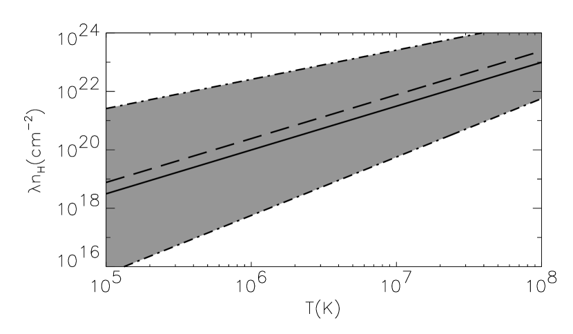
Figure 1: Critical wavelengths and boundaries of the sound domain. The solid line indicates the critical wavelength for the condensation mode. The dashed line corresponds to the critical wavelength for the sound waves. The two dash–dotted lines are the points where $\tau_{c}^{-1}=\omega_{s}$ (upper straight) and $\tau_{\chi}^{-1}=\omega_{s}$ (lower straight): the sound domain, therefore, is contained within the shaded band.

(b) Comparison of WKB- and exact solutions. We consider both the condensation mode and the sound waves for a case defined by $\lambda{n_{H}}=10^{21}\,$cm^-2 and $T_{0}=7.3\times 10^{6}\,$K at $t=0$ (Fig. 2). With this choice, both modes have initially a wavelength below the critical value. Figures 2a and b show the time evolution of the background temperature and of $|\Omega_{cp}|/\omega_{s}$ and $\tau_{\chi}^{-1}/\omega_{s}$. The other four panels in the figure compare the WKB solution with the numerical solution of the linear system (15)-(17) for an initial amplitude of the perturbation $\rho_{1}/\rho_{0}=0.01$. Panels (c), (d) and (e) show the time evolution of the condensation mode (solid: WKB approximation; dashed: numerical solution) and the relative error between them (dotted line). The WKB solution turns out to be an excellent approximation to the exact solution: both curves are almost indistinguishable except when $|\Omega_{cp}|\sim\omega_{s}$. In fact, the relative error of the WKB solution for $\rho_{1}/\rho_{0}$ is still below $0.01$ when $|\Omega_{cp}|/\omega_{s}$ reaches the value $0.1$. Initially, the condensation mode has a wavelength below the critical value, but the latter decreases as the system cools (see Fig. 1) and their ratio grows above unity for $t/{\tau_{s}}_{0}=12$. Therefore, $\rho_{1}/\rho_{0}$ first decreases, then reaches a minimum at that time, and grows thereafter. Figure 2f shows the WKB and numerical solutions for the sound wave. Again, the agreement between both solutions is excellent. The wavelength ratio follows a similar evolution as for the condensation mode, and so does the perturbation amplitude.

Figure 2: Comparison of the WKB and the numerical solutions for the condensation and sound modes. (a) Evolution of the background temperature. (b) Solid line: time evolution of $|\Omega_{cp}|/\omega_{s}$. Dashed line: evolution of $\tau_{\chi}^{-1}/\omega_{s}$. (c), (d), and (e) show the evolution of the condensation mode: the solid line is the WKB solution and the dashed line is the numerical solution (in panel d, they coincide within the resolution of the figure). Panel (f) shows the evolution of the density perturbation for a sound wave (again, WKB and numerical solution coincide in the figure). Panels (c), (d) and (f) also show, as a dotted line, the relative error between the numerical and the WKB solutions.

3.2 Solutions on Scales around the Jeans Length: the Acoustic–Gravity Domain without Background Expansion

Going to spatial scales larger than in the foregoing section, there is interesting new physics when the wavelength approaches the Jeans length, $L_{J}=2\pi c_{s}/\omega_{g}\,$, that is, as soon as $\omega_{g}$ is no longer small compared to $\omega_{s}$. In this subsection we study the regime in which either sound or gravity (or both simultaneously) are dominant and the background is slowly cooling or heating but with zero expansion rate (if $\dot{a}\neq 0$, the expansion would become as dominant as self-gravity itself after a time of order $\tau_{g}$ at the latest, see eq. [9], and the WKB model could not be used).

Consider, then, the case in which $|\Omega_{dc}|$, $\tau_{c}^{-1}$ and ${\tau_{\chi}}^{-1}$ are all much smaller than both $\omega_{s}$ and $\omega_{g}$. There are then three WKB solutions: two acoustic–gravity modes and a condensation mode. We use the symbols ${\psi_{ag}}_{\pm}$ and $\psi_{c}$ for their respective growth rates for $\rho_{1}/\rho_{0}$. As in the previous case, the zero-order solutions are obtained by calculating the three roots of the polynomial (34), but now the coefficients $A_{i}$, $B_{i}$ and $C_{i}$ have the values given in Appendix A.2, expressions (A5). The result is:

$$\omega_{0}{\psi_{0ag}}_{\pm} = \pm i\sqrt{\omega_{s}^{2}-\omega_{g}^{2}}\;$$ (49)

                               and

$$\psi_{0c} = 0\;.$$ (50)

To zero order, therefore, we have a couple of acoustic–gravity modes (eq. [49]) like those obtained by Jeans (1902) and a non-evolving mode (eq. [50]). The latter corresponds to any perturbation with $v_{1}=0$ and $p_{1}/p_{0}=\gamma(\omega_{g}^{2}/\omega_{s}^{2})\rho_{1}/\rho_{0}$, i.e., equilibrium between pressure gradient and self-gravity. If $\omega_{g}<\omega_{s}$ the acoustic–gravity modes are waves. They have a frequency smaller than a pure sound wave with the same wavelength because the self-gravity force acts against the pressure gradient force. If $\omega_{g}>\omega_{s}$ these modes grow or decay exponentially. In the growing mode, in particular, the perturbation collapses gravitationally and the pressure gradient is not large enough to prevent it. The introduction of cooling and thermal conduction as non-dominant processes makes the amplitude of these modes change. These modifications are given by the WKB corrections of order one and greater.

To calculate the first order corrections for the growth rates of $\rho_{1}/\rho_{0}$ for those modes, namely ${\psi_{1ag}}_{\pm}$ and $\psi_{1c}$, we turn again to the general WKB solution (eq. [2.5]), using $n=1$ and the coefficients given in expressions (A6) of Appendix A.2. We show and discuss them in the following:

3.2.1 Condensation Mode

The first order WKB correction for the condensation mode is given by

$$\psi_{1c}=-\frac{(\gamma-1)}{\gamma}\frac{\mu}{{\cal R}}\left\{T_{0}\left[\frac{\partial}{\partial T}\left(\frac{\mathcal{L}}{T}\right)\right]_{p}-\gamma\frac{\omega_{g}^{2}}{\omega_{s}^{2}}\left(\frac{\partial\mathcal{L}}{\partial T}\right)_{\rho}+\frac{\chi_{0}}{\rho_{0}}\frac{k^{2}}{a^{2}}\left(1-\gamma\frac{\omega_{g}^{2}}{\omega_{s}^{2}}\right)\right\}\left(1-\frac{\omega_{g}^{2}}{\omega_{s}^{2}}\right)^{-1}\;.$$ (51)

This mode reduces to the sound domain condensation mode (40) when $\omega_{g}\ll\omega_{s}$. We introduce the quantity

$$F=\frac{p_{1}}{p_{0}}-\gamma\frac{\omega_{g}^{2}}{\omega_{s}^{2}}\frac{\rho_{1}}{\rho_{0}}\;,$$ (52)

which is proportional to the perturbation of the net volume force (pressure gradient minus self-gravity). Using this quantity, the relative perturbations can be written

$$\frac{v_{1}}{c_{s}}=\frac{i\psi_{1c}}{\omega_{s}}\;\frac{\rho_{1}}{\rho_{0}}\sim{\cal O}\left(\frac{\omega_{1}}{\omega_{s}}\right)\;\frac{\rho_{1}}{\rho_{0}}\;,\qquad F=-\gamma\frac{\dot{\psi}_{1c}+\psi_{1c}^{2}}{\omega_{s}^{2}}\frac{\rho_{1}}{\rho_{0}}\sim{\cal O}\left(\frac{\displaystyle\omega_{1}^{2}}{\displaystyle\omega_{s}^{2}}\right)\frac{\rho_{1}}{\rho_{0}}\;,$$ (53)

where $\omega_{1}$ is the inverse time-scale of the non-dominant processes (conduction and cooling). This is similar to equation (41) but now the sound-gravity modes, that propagate or grow much faster than the condensation mode, lead to the cancellation of the gravity force by the pressure gradient instead of to a condition of uniform pressure throughout.

The first order correction (51) shows three interesting features. First, it diverges when $\omega_{s}=\omega_{g}$, i.e., there is a turning-point in the WKB sense. The turning point can easily be reached in a cooling and non-expanding medium for wavelengths for which, initially, $\omega_{s}>\omega_{g}$: the former frequency decreases with time whereas the latter stays constant. As known from the WKB theory, when a solution goes through a turning point, a mixing of modes takes place. Second, conduction has a destabilizing effect in the range $\gamma\omega_{g}^{2}>\omega_{s}^{2}>\omega_{g}^{2}\;$. This can be explained using the equation of evolution for the perturbed entropy, $S_{1}$, and the relation between $S_{1}$ and $T_{1}/T_{0}$ following the condition of permanent equilibrium between gravity and pressure gradient. Third, the combination of partial derivatives of $\mathcal{L}$ is quite different to the corresponding expression in equation (40). In the following we explain the origin of the last feature.

To explain the origin of the cooling terms in equation (51) we can use the results of Balbus (1986). Using Lagrangian perturbations in the entropy equation, he derived an instability criterion for the condensation mode in the absence of conduction in the particular case in which the perturbation of an arbitrary thermodynamic variable $A$ is kept equal to zero during the evolution of the condensation mode. The resulting criterion is obtained from the following equation:

$$\frac{1}{\Delta S}\frac{d\Delta S}{dt}=-\left[\frac{\partial}{\partial S}\left(\frac{\mathcal{L}}{T}\right)\right]_{A}\;,$$ (54)

where $\Delta$ indicates Lagrangian perturbation. Balbus (1986) applies this equation to the cases $A=p$ and $A=\rho$. In the present section, in turn, the physical quantity whose perturbation remains equal to zero is $F$ (eq. [53]); on the other hand, Lagrangian and Eulerian perturbations are indistinguishable since the background is uniform (e.g., Shapiro & Teukolsky, 1983). It can then be shown that the cooling terms in equation (51) can be derived from the right-hand side of equation (54), using the relationship between the growth rates of $S_{1}$ and $\rho_{1}/\rho_{0}$.

Critical lengths are computed solving the equation $\psi_{1c}=0$. This equation can be expressed as:

$$\frac{{\lambda_{crit}}^{4}}{L_{J}^{4}}+\left(\frac{{{\tau_{\chi}}_{J}}^{-1}}{{\Omega_{F}}}-\frac{1}{\gamma}\frac{\Omega_{cp}}{{\Omega_{F}}}\right)\frac{{\lambda_{crit}}^{2}}{L_{J}^{2}}-\frac{1}{\gamma}\frac{{{\tau_{\chi}}_{J}}^{-1}}{{\Omega_{F}}}=0$$ (55)

where ${\lambda_{crit}}$ is the critical wavelength, ${{\tau_{\chi}}_{J}}^{-1}$ is $\tau_{\chi}^{-1}$ evaluated for $\lambda=L_{J}$, and

$${\Omega_{F}}=(\gamma-1)\frac{\mu}{{\cal R}}\left(\frac{\partial\mathcal{L}}{\partial T}\right)_{\rho}\;,$$ (56)

i.e., minus the growth rate due to isochoric cooling in the classical theory of Field (1965). At the Jeans length, it is natural to expect cooling to be much faster than conduction (${{\tau_{\chi}}_{J}}^{-1}\ll{\Omega_{F}}$). Assuming this, the solutions of equation (55) are given by:

$${{\lambda_{crit}}^{2}}_{1}=-\frac{{{\tau_{\chi}}_{J}}^{-1}}{\Omega_{cp}}L_{J}^{2}\qquad\hbox{and}\qquad{{\lambda_{crit}}^{2}}_{2}=\frac{1}{\gamma}\frac{\Omega_{cp}}{{\Omega_{F}}}L_{J}^{2}\;.$$ (57)

For the existence of a critical length, the right-hand side of the corresponding expression must be positive. The first critical length coincides with that of equation (46), which corresponds to a condensation mode in the sound dominated case. The second critical length is new, and has a value that is near $L_{J}$. If both critical lengths exist and ${\lambda_{crit}}_{1,2}/L_{J}<1$, the condensation mode will be unstable for wavelengths $\lambda$ such that ${\lambda_{crit}}_{1}<\lambda<{\lambda_{crit}}_{2}$.

3.2.2 Acoustic–Gravity Modes

The first order WKB correction for the acoustic–gravity modes is

$${\psi_{1ag}}_{\pm}=-\frac{(\gamma-1)}{2}\frac{\mu}{{\cal R}}\left\{\frac{\gamma-1}{\gamma}\left[\left(\frac{\partial\mathcal{L}}{\partial T}\right)_{S}+\frac{\chi_{0}}{\rho_{0}}\frac{k^{2}}{a^{2}}\right]-\left(\frac{3}{2}-\frac{1}{\gamma}\right)\frac{\mathcal{L}_{0}}{T_{0}}\right\}\left(1-\frac{\omega_{g}^{2}}{\omega_{s}^{2}}\right)^{-1}\;.$$ (58)

This term coincides with the first-order correction for the sound waves given in equation (42) for zero background expansion but divided by $1-\omega_{g}^{2}/\omega_{s}^{2}$. For $\omega_{g}<\omega_{s}$, this is not surprising because the acoustic–gravity waves behave in that case like sound waves of the same wavelength but with a smaller frequency. Similarly as for the sound domain, for this mode there is only one critical wavelength, obtained solving $\psi_{1ag}=0$.

4 THE SHORT– AND LONG–WAVELENGTH RANGES

For completeness (and later use in section 5), we briefly discuss in this section two results for perturbations in the conduction and cooling domains.

4.1 Small Spatial Scale: Heat Conduction Domain

At small enough spatial scale (a) thermal conduction is the dominant process and (b) $\omega_{s}^{-1}$ is much smaller than $\tau_{g}$, $\tau_{e}$ and $\tau_{c}$, so that ${\tau_{\chi}}\ll\omega_{\rm{s}}^{-1}\ll\min(\tau_{g},\;\tau_{e},\;\tau_{c})$. Two simple consequences of the foregoing are: (1) conduction can eliminate any temperature gradients well before the sound waves can cross a wavelength and (2) the evolution of the dominant processes (conduction and sound propagation) occurs without important evolution of the background through cooling and expansion. The solutions to zero and first WKB order must thus coincide with the solutions obtained by Field (1965), viz. a condensation mode at zero order and quasi-isothermal sound waves at first order. The condensation mode evolves on the timescale of the thermal conduction, ${\tau_{\chi}}$. Using this fact in equations (15)–(17) one obtains $v_{1}/c_{s}\sim{\cal O}(\omega_{s}/\tau_{\chi}^{-1})\;p_{1}/p_{0}\;$, $\rho_{1}/\rho_{0}\sim{\cal O}(\omega_{s}^{2}/\tau_{\chi}^{-2})\;p_{1}/p_{0}$ and

$$\frac{\displaystyle d}{\displaystyle dt}\left(\frac{p_{1}}{p_{0}}\right)=-\frac{\displaystyle 1}{\displaystyle{\tau_{\chi}}}\frac{\displaystyle p_{1}}{\displaystyle p_{0}}\quad.$$ (59)

The condensation mode at small length-scales is therefore completely stabilized by conduction. As a consequence of the smallness of $\rho_{1}/\rho_{0}$, to obtain the WKB solutions for this mode it is necessary to use a third order differential equation for $p_{1}/p_{0}$ instead of the differential equation (28) for $\rho_{1}/\rho_{0}$.

4.2 Large Spatial Scale: Cooling Domain

At large enough wavelength, cooling, expansion and/or self-gravity dominate, so that the following ordering of timescales applies: $\min{(\tau_{g},\;\tau_{e},\;\tau_{c})}\ll\omega_{\rm{s}}^{-1}\ll{\tau_{\chi}}$. Whenever cooling or expansion dominate, no WKB solutions can be calculated, since in that case background and perturbation evolve on the same or comparable timescales. However, a zero order solution can be obtained by direct inspection of equations (15) through (17) when there is a single dominant process. For instance, if cooling is the single dominant process, we expect the zero order solution to have a growth rate of order $\tau_{mc}^{-1}=\max{(\tau_{c}^{-1},\Omega_{dc})}$ for all relative perturbations $\rho_{1}/\rho_{0}$, $v_{1}/c_{s}$ and $p_{1}/p_{0}$. Inserting that timescale into equations (15)-(17) one finds: $v_{1}/c_{s}\sim{\cal O}(\omega_{s}/\tau_{mc}^{-1})\;p_{1}/p_{0}$ and $\rho_{1}/\rho_{0}\sim{\cal O}(\omega_{s}^{2}/\tau_{mc}^{-2})\;p_{1}/p_{0}$. This perturbation evolves at almost constant density because the propagation of sound is much slower than the growth by cooling. The growth rate at zero order can be obtained from the previous considerations and equations (17) and (20):

$$\frac{d}{dt}\left(\frac{p_{1}}{p_{0}}\right)=-\Omega_{c\rho}\;\left(\frac{\displaystyle p_{1}}{\displaystyle p_{0}}\right)\;.$$ (60)

Balbus (1986) obtained this growth rate for the perturbed entropy using equation (54) with $A=\rho$.

5 GENERALIZED FIELD LENGTH IN AN ASTROPHYSICAL COOLING MEDIUM

We consider the thermal stability of an optically thin astrophysical medium at a temperature in the range $10^{4}-10^{8}$K which is undergoing net cooling. The medium is assumed to be uniform (or only weakly non-uniform in the sense of eq. [36]). Old SNRs and super-bubbles are examples of such a medium. The generalized Field length, which can be computed using the results of section 3.1.3, separates the stable regions from the unstable ones in wavenumber Fourier space. Self-gravity can be ignored because for the considered medium the Jeans length is usually much larger than the Field one. Assuming no heating and permanent ionization equilibrium, the cooling function only depends on the instantaneous properties of the medium and can be expressed as follows:

$$\mathcal{L}=\left(\frac{n_{e}n_{H}}{\rho^{2}}\right)\rho\,\Lambda(T)\;,$$ (61)

where $n_{e}$ is the electron number density, $n_{H}$ is the total number density of hydrogen (atoms and ions) and $\Lambda$ is a function that only depends on temperature. We use the function $\Lambda(T)$ provided by J. C. Raymond (2001, private communication) for standard abundances and $n_{H}=1\,$cm^-3 (see Fig. 3), which is an improved version of the cooling function of Raymond, Cox & Smith (1976). For $T<3\times 10^{4}\,$K, the function $\Lambda(T)$ has a very weak dependence on $n_{H}$, which can be safely neglected in the present context. In the considered temperature range, $\gamma=5/3$ and the thermal conduction coefficient, $\chi$, is given by equation (48). A number of authors have suggested a substantial reduction of $\chi$ in the Intergalactic Medium due to, for instance, kinetic instabilities driven by temperature gradients (e.g., Pistinner, Levinson & Eichler, 1996), a tangled magnetic field, which makes the effective mean free path of electrons smaller (e.g., Rosner & Tucker, 1989) and may cause magnetic mirroring (e.g., Chandran et al., 1999). Thus, as is usual, we include a constant factor $\xi$, with value between $0$ and $1$, multiplying the conduction coefficient $\chi$.

Figure 3: Cooling function $\Lambda(T)$ of J. C. Raymond (2001, private communication) for standard abundances.

5.1 Unmagnetized Background

The generalized Field length, ${\lambda_{crit}}$, can be calculated inserting the cooling function (61) into the growth rates (40) and (42) for the condensation and sound modes, respectively, and setting them equal to zero. The result is:

$${\lambda_{crit}}^{2}\,n_{H}^{2}\,x\,=\,4\pi^{2}\,\xi\,\chi\,\frac{T}{\Lambda(T)}\,\left[\alpha-\frac{d\log{\Lambda}}{d\log{T}}\right]^{-1}\;,$$ (62)

with $\alpha=2$ for the condensation mode and $\alpha=3/4$ for the sound waves. In equation (62), $x=n_{e}/n_{H}$ and all quantities are evaluated in the background. If the logarithmic temperature gradient of $\Lambda$ is positive and steep enough, the right-hand side of equation (62) becomes negative and there is no critical length: the corresponding mode is stable at that temperature for all wavelengths.

It is instructive to compare equation (62) with the classical Field length (sec. 3.1.3), i.e., the critical length if the background were in thermal equilibrium through the action of a heating which exactly compensates the cooling. Since we are interested primarily in the destabilizing effect of the cooling, we assume a density– and temperature–independent heating. The classical Field length is also given by equation (62) but with $\alpha=1$ for the condensation mode and $\alpha=-3/2$ for the sound waves. From these values of $\alpha$, comparing them with the values obtained above (see Fig. 4), we gather that there are more (and wider) unstable temperature ranges in the case with net background cooling than in the classical Field problem. In fact, the difference is quite striking for the sound waves, which change from stable to unstable almost everywhere if one suppresses the heating providing thermal equilibrium.

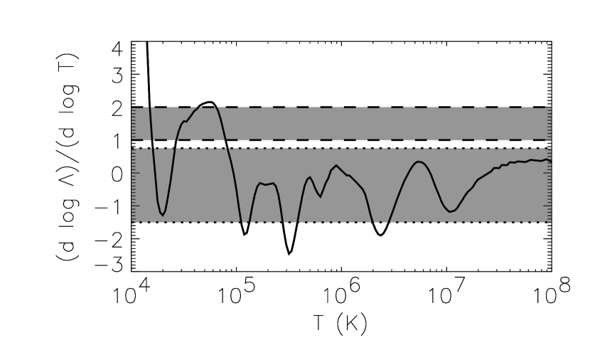
Figure 4: The solid line shows $(d\log{\Lambda})/(d\log{T})$ for the function $\Lambda(T)$ represented in Figure 3. The horizontal lines give the upper limits of existence of a critical length for the condensation mode (dashed) and for the sound waves (dotted), whereby in both cases the lower line corresponds to the Field problem and the upper one to the case with net background cooling. Wherever the solid line falls onto the shaded bands, the system with net background cooling is unstable whereas the results for thermal equilibrium predict stability.

Figure 5 shows the instability regions and the critical lengths in the two–dimensional parameter space ($T$, $\lambda\,n_{H}\,x^{1/2}\,\xi^{-1/2}$). The upper diagram corresponds to the sound waves, the lower one to the condensation mode. In the dark–grey shaded region, both the classical Field problem and the case with net background cooling are unstable, whereas in the light–grey shaded region only the latter is unstable. As expected, the instability region for the sound waves is much larger for the case with net background cooling. For the condensation mode, both regions are comparable, but, again, the range of unstable temperatures is smaller for the classical Field problem. In fact, the ranges of instability for sound waves and condensation mode are similar when there is net background cooling, which is in strong contrast to the situation in the classical Field problem. The upper left corner of each diagram corresponds to a region where cooling is dominant (i.e., it occurs on the fastest time-scale of the problem). Hence, there are no properly defined sound waves in that region (hatched area in the upper diagram).

The critical length expression (62) is valid only when sound is the dominant process, which happens within the region delimited by the curves $\omega_{s}=\tau_{\chi}^{-1}$ (dotted line) and $\omega_{s}=\tau_{c}^{-1}$ (dash–dotted line) in the diagram. However, we know that the region below the $\omega_{s}=\tau_{\chi}^{-1}$ – line is stable, since conduction is dominant. Similarly, in the cooling-dominated region (i.e., well above the dash-dotted line), where conduction is negligible, we know the instability properties of the condensation mode both for the classical Field problem and for the case with net background cooling using an isochoric criterion as explained in section 4.2. The remaining unknown region is, thus, a (possibly narrow) band around the $\omega_{s}=\tau_{c}^{-1}$ – line. We have tentatively indicated this band in the figure as a cross–hatched region. As a final remark, note that the use of the parameter $\lambda\,n_{H}\,x^{1/2}\,\xi^{-1/2}$ in the figure is meaningful because we have ignored the weak dependence of the Coulomb logarithm on $n_{e}$ (see eq. [48]). For the figure, $n_{e}$ has been set equal to $1$cm^-3 in $\Lambda_{C}$.

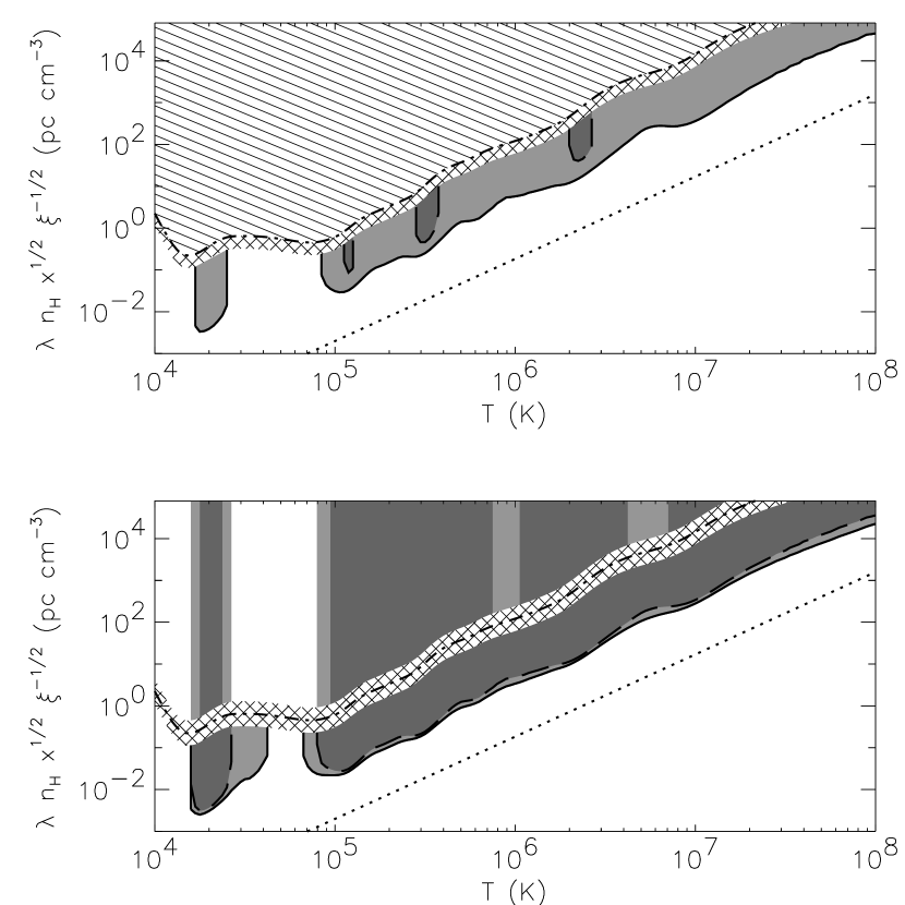
Figure 5: Critical wavelengths and regions of instability for the sound waves (upper panel) and the condensation mode (lower panel) for the application discussed in section 5. The critical wavelength ${\lambda_{crit}}$ is plotted as a solid line for the case with net background cooling and as a dashed line for the classical Field problem. The dark-grey shaded area is the region where both problems yield instability; in the light-grey shaded region only the case with net background cooling is unstable. In the upper left corner of the upper panel (hatched area in the figure) the sound waves are not properly defined so that no statement concerning their stability is possible there. Two further lines depicted in the figure are the locus of points where $\omega_{s}=\tau_{\chi}^{-1}$, with $\xi=1$ and $x=1$ (dotted) and those where $\omega_{s}=\tau_{c}^{-1}$, with $\xi=1$ and $x=1$ (dash-dotted line). The stability of the points in the figure in a narrow band around the dash-dotted line (indicated with cross hatching) is uncertain, as explained in the text.

5.2 Inclusion of a Background Magnetic Field without Dynamical Effects

The astrophysical media considered in the previous subsection (like the hot interstellar medium or the intergalactic medium) are threaded by magnetic fields. Usually, these fields are dynamically unimportant, that is, in these media $\beta>>1$, where $\beta$ is the ratio of thermal and magnetic pressures. However, the effect of this weak magnetic field on thermal conduction is very strong. Therefore, we include such a weak magnetic field to complete the discussion of the previous paragraph. In a medium threaded by a magnetic field, the growth rate of $\rho_{1}/\rho_{0}$ for the condensation mode in the limit $\beta>>1$ is given by (A. J. Gomez-Pelaez & F. Moreno-Insertis, in preparation):

$$\psi_{1c}=-\frac{(\gamma-1)}{\gamma}\frac{\mu}{{\cal R}}\left\{T_{0}\left[\frac{\partial}{\partial T}\left(\frac{\mathcal{L}}{T}\right)\right]_{p}+\frac{1}{\rho_{0}}\frac{k^{2}}{a^{2}}\left[{\chi_{\parallel}}_{0}\cos^{2}{\theta}+{\chi_{\perp}}_{0}\sin^{2}{\theta}\right]\right\}\;,$$ (63)

where $\theta$ is the angle between the background magnetic field, $\bf{B_{0}}$, and the wavenumber vector $\bf{k}$, the conductivity parallel to the magnetic field, $\chi_{\parallel}$, is given by equation (48), and the perpendicular conductivity, $\chi_{\perp}$, is given by (Spitzer, 1962):

$$\frac{\chi_{\perp}}{\chi_{\parallel}}=7.2\times 10^{-16}\left(\frac{\log{\Lambda_{C}}}{30}\right)^{2}\frac{n_{i}^{2}}{B_{\mu G}^{2}T_{6}^{3}}\;,$$ (64)

in which $\log{\Lambda_{C}}$ is given by equation (48), $n_{i}$ is the number density of ions in cm^-3, $B_{\mu G}$ is the magnetic field in $\mu G$, and $T_{6}$ is the temperature measured in $10^{6}$K . Expression (64) is only applicable when the temperature of ions and electrons is the same and the Larmor radius of the ions is much smaller than their mean free path, which is always the case in the media considered in this section. The corresponding expression for the sound waves is:

$${\psi_{1s}}_{\pm} = -\frac{(\gamma-1)}{2}\frac{\mu}{{\cal R}}\left\{\frac{\gamma-1}{\gamma}\left[\left(\frac{\partial\mathcal{L}}{\partial T}\right)_{S}+\frac{1}{\rho_{0}}\frac{k^{2}}{a^{2}}\left({\chi_{\parallel}}_{0}\cos^{2}{\theta}+{\chi_{\perp}}_{0}\sin^{2}{\theta}\right)\right]\right.$$ (65)

$$- \left.\left(\frac{3}{2}-\frac{1}{\gamma}\right)\frac{\mathcal{L}_{0}}{T_{0}}\right\}+\frac{(3\gamma-5)}{4}\frac{\dot{a}}{a}\;,$$

In the limit $\beta>>1$, the only effect of the magnetic field is to make the thermal conduction depend on the spatial direction. The growth rate of both modes, and therefore their associated generalized Field lengths (${\lambda_{crit}}$), depend on $\theta$. Setting both, $\psi_{1c}$ (eq. [63]) and ${\psi_{1s}}_{\pm}$ (eq. [65]), equal to zero, one obtains

$${\lambda_{crit}}(\theta)={\lambda_{crit}}_{\parallel}\left(\cos^{2}{\theta}+\frac{\chi_{\perp}}{\chi_{\parallel}}\sin^{2}{\theta}\right)^{1/2},$$ (66)

where ${\lambda_{crit}}_{\parallel}$, is given by equation (62). We will also use the symbol ${\lambda_{crit}}_{\perp}$ for ${\lambda_{crit}}(\theta=\pi/2)$.

Figure 6 shows the generalized (solid line) and classical (dashed line) Field length and the instability regions for the condensation and sound modes with $\theta=\pi/2$. The upper diagram corresponds to the sound waves, the lower one to the condensation mode. Here again, dark-grey shading indicates that both the thermal equilibrium problem and the case with net background cooling are unstable; in the light-grey shaded area only the latter is unstable. Note that now the combination $\lambda\,B_{\mu G}\,x^{-1/2}$ appears in ordinates, since ${\lambda_{crit}}_{\perp}$ does not depend on $n_{H}$ but on $B_{\mu G}$. From the figure (compare with Figure 5), it is apparent that ${\lambda_{crit}}_{\perp}<<{\lambda_{crit}}_{\parallel}$ and that ${\lambda_{crit}}_{\perp}$ has a weaker dependence on temperature than ${\lambda_{crit}}_{\parallel}$. Both features are a direct consequence of the conductivity ratio (64). Hence, if there is a background magnetic field, the condensations, in the linear stage, will be filaments directed along the magnetic field lines with a length of the same order as ${\lambda_{crit}}_{\parallel}$ and a diameter of the same order as ${\lambda_{crit}}_{\perp}$.

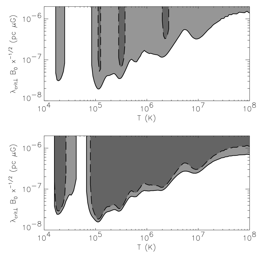
Figure 6: Perpendicular Field length, ${\lambda_{crit}}_{\perp}$, and regions of instability for a magnetized medium with $\beta\gg 1$ for the sound waves (upper panel) and the condensation mode (lower panel). ${\lambda_{crit}}_{\perp}$ is plotted as a solid line for the case with net background cooling and as a dashed line for the classical Field problem. In the dark-grey shaded areas both the thermal equilibrium problem and the case with net background cooling are unstable; in the light-grey shaded area only the latter is unstable.

Typical values of the critical length in the hot interstellar medium (as inside SNRs and superbubbles) follow from the physical parameters in them like: $n_{H}=10^{-3}\;$cm^-3, $T=10^{6}\;$K, and $B_{\mu G}=1$ (e.g., McKee, 1995). The associated critical lengths are: (1) ${\lambda_{crit}}_{\parallel}=3.4\;$kpc and ${\lambda_{crit}}_{\perp}=9\times 10^{-8}\;$pc for the condensation mode and (2) ${\lambda_{crit}}_{\parallel}=6\;$kpc and ${\lambda_{crit}}_{\perp}=1.5\times 10^{-7}\;$pc for the sound waves. Note that ${\lambda_{crit}}_{\parallel}$ is larger or of the same order than the size of the considered systems whereas ${\lambda_{crit}}_{\perp}$ is well below it.

6 SUMMARY AND DISCUSSION

We have carried out a systematic analysis of the thermal stability of a uniform medium which, in the unperturbed state, is undergoing net cooling and expansion, so that the problem is not amenable to a full Fourier normal mode analysis. Thermal conduction and self-gravity have also been included as fundamental ingredients. The small-perturbation problem yields a system of ordinary differential equations with three independent solutions. In many cases, two of them have the character of oscillatory modes (typically sound waves, or, more generally, acoustic-gravity modes) and the third one is a non-oscillatory (or condensation) solution. The wavelength of the perturbation determines the positions of the different physical processes in the hierarchy of timescales. At small enough wavelength, thermal conduction damps the condensation mode and makes sound waves isothermal. At large wavelength, one or a few of the following processes are dominant: cooling, self-gravity and expansion. For example, if cooling is the only dominant process, the perturbation evolving on the fastest timescale is isochoric with no sound waves present that could even out the pressure gradients. At intermediate wavelength, the propagation of sound is the fastest process, so the evolution of the condensation mode is isobaric. In the paper, solutions have been obtained in a number of instances using the WKB method. WKB solutions can be found only if two conditions are fulfilled: (1) there is a clear separation of timescales between fast and slow physical processes in the system, and (2) the background expansion and cooling belong to the slow category.

Of special interest in this paper are those solutions whose growth rate is of the same order as the rate of change of the unperturbed background. In this case, the change in time of the critical wavelengths (the generalized Field length, ${\lambda_{crit}}$, and the Jeans length, $L_{J}$) may make the perturbation go through totally different stability regimes during their evolution. For example, the solutions obtained in section 3.2 for a medium undergoing net cooling include a condensation mode initially in the stable range whose wavelength becomes larger than the Field length after some time, thus becoming thermally unstable. Later on, the Jeans length decreases sufficiently so that the perturbation also becomes gravitationally unstable. A sound wave may undergo a similar process of change of stability, first being in a stable regime with slowly decreasing amplitude, then becoming thermally unstable and finally, when the self-gravity frequency becomes comparable with the sound frequency, turning into an acoustic-gravity mode which ends up as a gravitationally-dominated perturbation.

The analysis of the present paper shows (section 5) that in a medium undergoing a realistic net cooling the sound waves are thermally unstable for a comparable range of wavelengths and temperatures as the condensation mode. This may come as a surprise: in contrast, and by way of example, if the thermal equilibrium is reached by balancing the cooling with a constant heating, the sound waves are stable for almost all temperatures in the range $10^{4}$ – $10^{8}$ whereas the condensation mode continues being unstable. On the other hand, the inclusion of a weak magnetic field has a strong influence on the thermal conduction. For astrophysical environments such as the hot ISM and the hot IGM, the generalized Field length along the magnetic field is many orders of magnitude larger than in the perpendicular direction. Therefore, the unstable condensations will be filaments directed along the magnetic field lines.

For the description of the astrophysical systems in which thermal instabilities appear, it is important to study the non-linear phase of both condensation mode and sound waves. The unstable sound waves develop pairs of shock fronts and rarefaction waves, as known from elementary hydrodynamics. The condensation mode, instead, just continues growing without propagating. The detailed physics of the nonlinear phase has to be calculated, in general, using numerical means. Yet, a number of results can be advanced at this stage. For instance, in the linear analysis, a perturbation with negative $\rho_{1}/\rho_{0}$ grows (in absolute value) as fast as a perturbation with positive $\rho_{1}/\rho_{0}$. This symmetry is broken in the non-linear evolution. In a medium undergoing net cooling, for example, a condensation with positive $\rho_{1}/\rho_{0}$ (negative $T_{1}/T_{0}$) grows faster than one with $\rho_{1}/\rho_{0}<0$. This happens because of the sum of the following two processes. First, thermal conduction grows with temperature. Therefore, a condensation with positive $T_{1}/T_{0}$ is more damped by thermal conduction than a negative one. Second, in the range $10^{5}-10^{7}$ cooling increases toward lower temperatures (Fig. 3). Therefore, a condensation with negative $T_{1}/T_{0}$ is more destabilized by cooling than a positive one. A related aspect is that the characteristic spatial size (width at half height) of a condensation decreases by orders of magnitude during its evolution. This happens because the coldest zones of the perturbation cool much faster than the warmer ones. The last aspect can be seen in the paper of David, Bregman & Seab (1988), where the non-linear evolution of a perturbation of this type is computed numerically.

In the weakly–magnetized case, at the beginning of the non-linear evolution ($\beta\gg 1$), the compression in the filament proceeds mainly in the directions perpendicular to the magnetic field lines. This is because of the reduction of thermal conduction transversely to the field lines: a much higher temperature (and thus pressure) gradient can be maintained across than along the field lines. The plasma $\beta$ inside the condensation decreases with time because of the temperature decrease and the growth of magnetic field due to the compression. In the advanced non-linear phase, the perpendicular compression comes to a halt once $\beta\ll 1$, since then the net force across the field lines (the gradient of the sum of magnetic and thermal pressures) is almost decoupled from temperature. After this, the compression is only possible along the field lines. As a related example, see David & Bregman (1989), which numerically compute the non-linear evolution of a planar condensation taking into account magnetic pressure.

The WKB analysis that we have carried out in this paper assumes a uniform background. However, our results are also applicable for a weakly non-uniform background. More in detail, our results for the condensation mode in the sound domain are valid if the Brunt-Väisälä frequency associated with the background entropy gradient is much smaller than the growth rate of the condensation mode. This holds, for example, in the supersonic region of a wind and inside old SNRs and superbubbles. In contrast, for the study of the thermal instability in cooling flows in clusters of galaxies, the buoyancy of the perturbations must be taken into account. Many authors have studied this problem: Mathews & Bregman (1978), Malagoli, Rosner & Bodo (1987), Balbus & Soker (1989), Loewenstein (1990) and Balbus (1991). Loewenstein (1990) and Balbus (1991), in particular, conclude that a magnetic field, even a weak one, can inhibit buoyancy and trigger thermal instability, which otherwise would be small due to buoyancy. The extension of the results of the present paper to environments of this type requires additional work.

Appendix A COEFFICIENTS FOR THE WKB SOLUTION

A.1 Coefficients for the Sound Domain

For the sound domain case (see sec. 3.1), the different order components of the coefficients $A(t)$, $B(t)$, and $C(t)$, have the value:

$$A_{3}=0\;,\quad B_{2}=\omega_{s}^{2}\;,\quad C_{1}=0\;,$$ (A1)

$$A_{2}=\frac{\omega_{s}^{2}}{\gamma}\left(\Omega_{cp}+{\tau_{\chi}}^{-1}\right)\;,\quad B_{1}=0\;,\quad C_{0}=\Omega_{c}+\Omega_{c\rho}+{\tau_{\chi}}^{-1}+(3\gamma+1)\frac{\dot{a}}{a}\;,$$ (A2)

$$A_{1}=0\;,\quad A_{0}=\omega_{g}^{2}\left[(4-3\gamma)\frac{\dot{a}}{a}-\Omega_{c}-\Omega_{c\rho}-{\tau_{\chi}}^{-1}\right]\;,$$ (A3)

$$B_{0}=2\frac{\ddot{a}}{a}-\omega_{g}^{2}-2\frac{\dot{a}}{a}\left[(2-3\gamma)\frac{\dot{a}}{a}-\Omega_{c}-\Omega_{c\rho}-{\tau_{\chi}}^{-1}\right]\;.$$ (A4)

A.2 Coefficients for the Sound and Self-Gravity Domain without Expansion

When sound and self-gravity dominate and there is no expansion (see sec. 3.2), the different order components of the coefficients $A(t)$, $B(t)$, and $C(t)$, have the value:

$$A_{3}=0\;,\quad B_{2}=\omega_{s}^{2}-\omega_{g}^{2}\;,\quad C_{1}=0\;,$$ (A5)

$$A_{2}=\frac{\omega_{s}^{2}}{\gamma}\left(\Omega_{cp}+{\tau_{\chi}}^{-1}\right)-\omega_{g}^{2}\left[\Omega_{c}+\Omega_{c\rho}+{\tau_{\chi}}^{-1}\right]\;,\quad B_{1}=0\;,\quad C_{0}=\Omega_{c}+\Omega_{c\rho}+{\tau_{\chi}}^{-1}\;.$$ (A6)

References

- Balbus (1986) Balbus, S. A. 1986, ApJ, 303, L79
- Balbus (1991) Balbus, S. A. 1991, ApJ, 372, 25
- Balbus & Soker (1989) Balbus, S. A., & Soker, N. 1989, ApJ, 341, 611
- Begelman & McKee (1990) Begelman, M. C., & McKee, C. F. 1990, ApJ, 358, 375
- Bender & Orszag (1978) Bender, C. M., & Orszag, S. A. 1978, Advanced Mathematical Methods for Scientist and Engineers (McGraw Hill: New York)
- Burkert & Lin (2000) Burkert, A., & Lin, D. N. C. 2000, ApJ, 537, 270
- Carrier, Krook & Pearson (1983) Carrier, G. F., Krook, M., & Pearson, C. E. 1983, Functions of a Complex Variable (New York: Hod Books)
- Chandran et al. (1999) Chandran, B.D.G., Cowley, S.C., Ivanushkina, M., Sydora, R. 1999, ApJ, 525,638
- Chun & Rosner (1993) Chun, E., & Rosner, R. 1993, ApJ, 408, 678
- David, Bregman & Seab (1988) David, L., Bregman, J., & Seab, G., 1988, ApJ, 329, 66
- David & Bregman (1989) David, L., & Bregman, J. 1989, ApJ, 337, 97
- Defouw (1970) Defouw, R. J. 1970, ApJ, 161, 55
- Fall & Rees (1985) Fall, S. M., Rees, M. J. 1985, ApJ, 298, 18
- Field (1965) Field, G. B. 1965, ApJ, 142, 531
- Flannery & Press (1979) Flannery, B. P., & Press, W. H. 1979, ApJ, 231, 688
- Goldsmith (1970) Goldsmith, D. 1970, ApJ, 161, 41
- Heyvaerts (1974) Heyvaerts, J. 1974, A&A, 37, 65
- Jeans (1902) Jeans, J. 1902, Phil Trans. 199A, 49 (4, 16)
- Loewenstein (1990) Loewenstein, M. 1990, ApJ, 349, 471
- Malagoli, Rosner & Bodo (1987) Malagoli, A., Rosner, R., & Bodo, G. 1987, ApJ, 319, 632
- Mathews & Bregman (1978) Mathews, W., & Bregman, J. 1978, ApJ, 224, 308
- McKee (1995) McKee, C. F. 1995, in ASP Conf. Ser. 80, The Physics of the Interstellar Medium and Intergalactic Medium, ed. A. Ferrara, C. F. McKee, C. Heiles, & P. R. Shapiro (San Francisco: ASP), 292
- Mihalas & Mihalas (1984) Mihalas, D., & Mihalas, B. W. 1984, Foundations of Radiation Hydrodynamics (Oxford: Oxford University Press)
- Parker (1953) Parker, E. N. 1953, ApJ, 117, 431
- Pistinner, Levinson & Eichler (1996) Pistinner, S., Levinson, A., & Eichler, D. 1996, ApJ, 467, 162
- Pistinner & Shaviv (1995) Pistinner, S., & Shaviv, G. 1995, ApJ, 448, L37
- Raymond, Cox & Smith (1976) Raymond, J. C., Cox, D. C., & Smith, B. W. 1976, ApJ, 204, 290
- Rosner & Tucker (1989) Rosner, R., & Tucker, W.H. 1989, ApJ, 338, 761
- Rybicki & Lightman (1979) Rybicki, G. B., & Lightman, A. P. 1979, Radiative Processes in Astrophysics (New York: Wiley)
- Shapiro & Teukolsky (1983) Shapiro, S., & Teukolsky, S. 1983, Black Holes, White Dwarfs and Neutron Stars (New York: Wiley)
- Spitzer (1962) Spitzer, L. 1962, Physics of Fully Ionized Gases (New York: Wiley)
- Weymann (1960) Weymann, R. 1960, ApJ, 132, 452