Astrometric and Light-travel Time Orbits to Detect Low-mass Companions: A Case Study of the Eclipsing System R Canis Majoris

Abstract

We discuss a method to determine orbital properties and masses of low-mass bodies orbiting eclipsing binaries. The analysis combines long-term eclipse timing modulations (light-travel time or LTT effect) with short-term, high-accuracy astrometry. As an illustration of the method, the results of a comprehensive study of Hipparcos astrometry and over a hundred years of eclipse timings of the Algol-type eclipsing binary R Canis Majoris are presented. A simultaneous solution of the astrometry and the LTTs yields an orbital period of $P_{12}=92.8\pm 1.3$ yr, an LTT semiamplitude of $2574\pm 57$ s, an angular semi-major axis of $a_{12}=117\pm 5$ mas, and values of the orbital eccentricity and inclination of $e_{12}=0.49\pm 0.05$, and $i_{12}=91.7\pm 4.7$ deg, respectively. Adopting the total mass of R CMa of $M_{12}=1.24\pm 0.05$ M_⊙, the mass of the third body is $M_{3}=0.34\pm 0.02$ M_⊙ and the semi-major axis of its orbit is $a_{3}=18.7\pm 1.7$ AU. From its mass, the third body is either a dM3-4 star or, more unlikely, a white dwarf. With the upcoming microarcsecond-level astrometric missions, the technique that we discuss can be successfully applied to detect and characterize long-period planetary-size objects and brown dwarfs around eclipsing binaries. Possibilities for extending the method to pulsating variables or stars with transiting planets are briefly addressed.

1. Introduction

Within the next decade several space astrometry missions, FAME and DIVA then SIM and GAIA, capable of sub-milli-arcsecond to micro-arcsecond accuracy are expected to be launched. One of the primary scientific goals of these missions is the astrometric detection of low mass objects around nearby stars, including brown dwarfs and Jupiter-sized planets. The detection of these objects will be accomplished through the observation of the reflex motion of the host star caused by the gravitational pull of the low-mass body. Although these missions are capable of very high astrometric accuracies and can observe up to millions of stars, their lifetimes are relatively short (2.5 to 5 yr). Thus, these space missions are optimized to detect planets within the habitable zones of late-type stars, but they could fail to detect (additional) planets with longer periods. It is important, however, to secure a complete picture of the bodies orbiting a star both from a pure census point of view and also to understand the genesis and evolution of planetary systems. In addition, planets do not necessarily remain within the habitable zone because of long-term chaotic perturbations. As we know from our Solar System, the presence of massive planets, such as Jupiter and Saturn, in distant orbits play a crucial role in stabilizing the orbits of the inner planets.

One effective way of extending the time baseline that permits the discovery of long period exosolar planets or brown dwarfs is to use the light-travel time (hereafter LTT) effect in eclipsing binaries. From this technique, the eclipses act as an accurate clock for detecting subtle variations in the distance to the object (this is analogous to the method used for discovering earth-sized objects around pulsars, see Wolszczan & Frail 1992). The periodic quasi-sinusoidal variations of the eclipse arrival times have a very simple and direct physical meaning: the total path that the light has to travel varies periodically as the eclipsing pair moves around the barycenter of the triple system. The amplitude of the variation is proportional both to the mass and to the period of the third body, as well as to the sine of the orbital inclination. As discussed by Demircan (2000), nearly 60 eclipsing binaries show evidence for nearby, unseen tertiary components using LTT effects. A recent example of a brown dwarf detected around the eclipsing binary V471 Tau using this method was presented by Guinan & Ribas (2001). Also this method is being employed in selected low mass eclipsing binaries to search for extrasolar planets (Deeg et al. 2000).

The primary advantages of using the LTT effect to detect third bodies in eclipsing binaries are: i) The necessary photometry can be secured with small telescopes using photoelectric or CCD detectors; ii) The number of eclipsing binaries is large – 4000 currently known in the Galaxy – and this number could increase very significantly when results from upcoming astrometry and photometry (e.g., MONS, COROT, Eddington, Kepler) missions are available; iii) For select eclipsing binaries (with sharp and deep eclipses) the timings can be determined with accuracies as good as several seconds; iv) The mass of the eclipsing pair can be known from conventional spectroscopic and light curve analyses. A shortcoming of the LTT method is that only upper limits to the mass and size of the orbit of the tertiary component can be determined (the analysis yields the mass function, $f(M_{3})$, and $a_{3}\sin i_{3}$). However, as it was demonstrated in the case of Algol (Bachmann & Hershey 1975), the LTT analysis can be complemented with astrometry to yield the orbital inclination and thus the actual mass and semi-major axis of the third body. Furthermore, with the orbital properties ($P$, $e$ and $\omega$) known from the LTT analysis, only a small fraction of the astrometric orbit needs to be covered when using high-accuracy astrometry.

In this paper we present the results of the combined LTT analysis and Hipparcos astrometry of the Algol-type eclipsing binary R CMa. The residuals of over 150 eclipse timings extending from 1887 to 2001 show a periodic ($\sim$93 yr) quasi-sinusoidal modulation. As previously shown by Radhakrishnan, Sarma, & Abhyankar (1984) and Demircan (2000), these variations are best explained by the LTT effect arising from the gravitational influence of a third body. The Hipparcos astrometry also shows the presence of small but significant acceleration terms in the proper motion components explicable by the reflex motion from a third body. Our study illustrates that with a well-defined LTT effect, only a few years of accurate astrometry are needed to constrain the orbital solution and determine the mass of the third body.

2. Overview of R CMa

R Canis Majoris (HD 57167, HR 2788, HIP 35487) is a bright ($V_{\rm max}=5.67$ mag), semi-detached eclipsing binary having an orbital period of 1.1359 days. As pointed out by Varricatt & Ashok (1999), R CMa holds special status among Algol systems in that it is the system with the lowest known total mass and hosting the least massive secondary star. Since the discovery of its variability in 1887 by Sawyer (1887), R CMa has been frequently observed and has well determined orbital and physical properties. The major breakthrough in understanding the system came when Tomkin (1985) was able to measure the very weak absorption lines of the faint secondary star and determine the masses of the two stars from a double line radial velocity study. The analyses of its light and radial velocity curves (see Varricatt & Ashok 1999) show that this system has a circular orbit and consists of a nearly spherical F0-1 V star ($M_{1}=1.07\pm 0.2$ M_⊙; $R_{1}=1.48\pm 0.10$ R_⊙; $L_{1}/{\rm L}_{\odot}=5.78\pm 0.38$) and a low mass, tidally-distorted K2-3 IV star ($M_{2}=0.17\pm 0.02$ M_⊙; $R_{2}=1.06\pm 0.07$ R_⊙; $L_{2}/{\rm L}_{\odot}=0.43\pm 0.10$). Moreover, nearly every photometric study indicates that the cooler star fills its inner Lagrangian surface. The relatively high space motions ($S=67$ km s^-1) suggest that R CMa is a member of the old disk population and thus a fairly old (5–7 Gyr) star (Guinan & Ianna 1983).

The present state of the system is best explained as a low mass Algol system that has undergone mass exchange and extensive mass loss. Asymmetries in its light curves and subtle spectroscopic anomalies indicate that mass exchange and loss are still continuing but at a much diminished rate compared to most Algol systems. The very low mass of the secondary star and old disk age indicate that R CMa is near the end of its life as an Algol system. As in the case of all Algol systems, the secondary star lies well above the main-sequence. However, unlike most Algol systems, the primary star is too hot and overluminous for observed mass. Moreover, a recent analysis of older photometry of R CMa by Mkrtichian & Gamarova (2000) indicates that the F star is a low-amplitude $\delta$ Scuti variable with a B light amplitude of 9 millimagnitudes and a period of 68 minutes.

3. Observations

3.1. Astrometry

Hipparcos observed R CMa between March 9, 1990 and March 5, 1993. There are 68 one-dimensional astrometric measurements corresponding to 35 different epochs in the Hipparcos Intermediate Astrometric Data, which were obtained by the two Hipparcos Data Reduction Consortia (33 measurements from FAST and 35 from NDAC). The astrometric data can be obtained from CD-ROM 5 of the Hipparcos catalog (ESA 1997). Unfortunately, the timespan of the Hipparcos observations is much smaller than the orbital period of the tertiary component, and this might eventually result in possible systematic errors in the orbital elements. To further constrain the solution additional older ground-based positions must be used. Indeed, Tycho-2 proper motions were computed by combining Tycho-2 positions and ground-based astrometric catalogs. For R CMa, 17 epoch positions of ground-based catalogs used for the Tycho-2 proper motion computation were kindly made available to us by Dr. Urban and are listed in Table 1. These measurements span over one century and so the Tycho-2 proper motions can be understood as the combination of the true proper motion and of a large fraction of the orbital motion. Consequently, the Tycho-2 proper motion of R CMa cannot itself be used in our analysis and only the individual positions contain valuable orbital information. In contrast, a short-term proper motion determination, such as the one computed around 1980 by Guinan & Ianna (1983), reveals itself to be very useful in constraining the astrometric solution.

In the course of the astrometric data reduction of the Hipparcos data, a test was applied to all the (apparently) single stars in order to check whether their motion was significantly non-linear. Most likely, a significant curvature of the photocenter motion is an indication of a possible duplicity. As it turns out, R CMa is one of the 2622 “acceleration” solutions of the Double and Multiple Stars Annex of the Hipparcos Catalogue, which provides a hint for the presence of a third body, independently from the LTT effect.

3.2. Photometry

R CMa has a long baseline of eclipse timings that extend from the present back to 1887. Most of the early eclipse times were determined from visual estimates. Several period studies have been carried out. Early studies of times of minimum light indicated a possible abrupt decrease in the period during 1914–15 (see Dugan & Wright 1939; Wood 1946; Koch 1960; Guinan 1977). However, as more timings accumulated it became apparent that the long-term variations in the (O–C)’s of the system are periodic and thus best explained by the LTT effect produced by the presence of a third body. The analysis of Radhakrishnan et al. (1984), with eclipse timings from 1887 to 1982, and Demircan (2000), who includes timings up to 1998, make a strong case in support of the LTT scenario.

Our photoelectric eclipse timing observations extend the time baseline up to early 2001. The observations were obtained with the Four College 0.8-m Automatic Photoelectric Telescope located in Southern Arizona during 1995/96 and 2000/01. Differential photometry was carried out using $uvby$ Strömgren filter sets. The mid-times of primary minimum and the (O–C)’s for these are given in Table 2, along with the corresponding uncertainties. The (O–C)’s were computed using a refined ephemeris determined from the analysis in §4 (Eq. 5). Our observations were combined with those compiled from the literature to yield a total of 158 eclipse timings from 1887 through 2001. The primary eclipse observations obtained from the literature are also provided in Table 2. Even though it is not explicitly mentioned in any of the publications, the times listed are commonly assumed to be in the UTC (coordinated universal time) scale. The timings were transformed from UTC to TT (terrestrial time) following the procedure described in Guinan & Ribas (2001), which is based on the recommendations of Bastian (2000). The timings listed in Table 2 are therefore HJD but in the TT scale.

The uncertainties of the individual timings are difficult to estimate. The compilation of Radhakrishnan et al. (1984) (from which most of the timings in Table 2 come) does not provide timing errors but only a relative weighting factor related to the quality of the data and the observation technique. We therefore adopted an iterative scheme to determine the actual uncertainties by forcing the $\chi^{2}$ of the (O–C) curve fit (in §4) to be equal to unity. This rather arbitrary scale factor determination is indeed justified because it ensures that the fitting algorithm will yield realistic uncertainties for the orbital parameters of the system. The individual timing errors are included in Table 2. The uncertainties yielded by the iterative scheme are about 10–13 minutes for photographic timings and some 2–4 minutes for photoelectric timings, in both cases reasonable figures given the characteristics of the two methods and the shape of the eclipse.

The Hipparcos mission, in addition to observing accurate positions of R CMa, obtained a total of 123 photometric measurements, which are present in the Hipparcos Epoch Photometric Data (ESA 1997). The phase coverage of the observations is not sufficient to determine an accurate primary eclipse timing using conventional methods. As an alternative, we adopted the physical information available to fit the entire light curve and derive a phase offset. Also, since the observations span 3 yr and the system exhibits (O–C) variations, the photometric dataset was split into two subgroups about January 1, 1991. Then, using the photometric elements of Varricatt & Ashok (1999), we employed the Wilson-Devinney program (Wilson & Devinney 1971) to run fits to both light curves by leaving only a phase shift and a magnitude zero point as free parameters. The fits were very satisfactory and we derived eclipse timings for the mean epochs from the best-fitting phase offsets. The resulting two timings, with uncertainties of around 100 s, are included in Table 2.

These two timings are significantly different as one would expect from the LTT secular change of period during the 3-year duration of the Hipparcos observations. More precisely, each date of observation could be approximated by $T\approx T_{\circ}+P_{\circ}E+gE^{2}$, with $E$ being the variability cycle number. So, the photometric “acceleration” term $g$ is a measure of the departure from a linear ephemeris during the observation window (the Hipparcos mission lifetime in this case). Since Hipparcos did not provide minimum timings, we used an alternative method to fit the equation above. The epoch measurements were folded using the reference epoch and period from ground-based studies. Then, the quadratic term was estimated by minimizing the distance between successive points of the folded light curve (string-length method). The fit yielded a value of $g=2.09\cdot 10^{-8}$ d, which leads to a cumulative effect of $gE_{\rm max}^{2}=0.0193\pm 0.0006$ d during the course of the Hipparcos observations. This rough estimation gives a significant acceleration term which is of the same order as that resulting from the long-term LTT analysis (§4) and indicates that the (O–C) variations attributed here to the presence of a third body could, in principle, have been detected through the Hipparcos photometric analysis alone.

4. Analysis

The expressions that describe the LTT effect as a function of the orbital properties were first provided by Irwin (1952). In short, the time delay or advance caused by the influence of a tertiary component can be expressed as:

$$\Delta T=\frac{a_{12}\sin i_{12}}{c}\left[\frac{1-e_{12}^{2}}{1+e_{12}\cos\nu_{12}}\sin(\nu_{12}+\omega_{12})+e_{12}\sin\omega_{12}\right]$$ (1)

where $c$ is the speed of light, and $a_{12}$, $i_{12}$, $e_{12}$, $\omega_{12}$, and $\nu_{12}$ are, respectively, the semi-major axis, the inclination, the eccentricity, the argument of the periastron, and the true anomaly (function of time) of the orbit of the eclipsing pair around the barycenter. As is customary, the orbital inclination $i_{12}$ is measured relative to the plane of the sky. The naming convention adopted throughout this paper uses subscripts 12 and 3 for the orbital parameters of the eclipsing pair and the tertiary component, respectively, around the common barycenter. Obviously, most of the parameters for the eclipsing pair’s and the third body’s orbits are identical (such as period, eccentricity, and inclination), but we use the subscript 12 because the actual measurements are made strictly for the brighter component of the long period system. Finally, subscript EB refers to the close orbit of the eclipsing binary.

The fit of Eq. (1) to the timing data would provide a good estimation of the a number of orbital and physical parameters of the system (see e.g., Guinan & Ribas 2001). However, both the orbital semi-major axis and the mass of the third body would be affected by a factor $\sin i$ that cannot be determined from the LTT analysis alone. When the LTT analysis is combined with astrometric data, all orbital parameters (including $i$ and even $\Omega$) can be determined yielding a full description of the system. The availability of Hipparcos intermediate astrometry permits the fitting of the observations using an astrometric model not accounted for in the standard Hipparcos astrometric solution. In the particular case of R CMa we have considered an orbital model that has been convolved with the astrometric motion (parallax and proper motion). The orbital motion produces the following effect on the coordinates:

$$\Delta x = a_{12}\;\frac{1-e_{12}^{2}}{1+e_{12}\cos\nu_{12}}[\cos(\nu_{12}+\omega_{12})\sin\Omega_{12}+$$ (2)

$$+\sin(\nu_{12}+\omega_{12})\cos\Omega_{12}\cos i_{12}]$$

$$\Delta y = a_{12}\;\frac{1-e_{12}^{2}}{1+e_{12}\cos\nu_{12}}[\cos(\nu_{12}+\omega_{12})\cos\Omega_{12}-$$ (3)

$$-\sin(\nu_{12}+\omega_{12})\sin\Omega_{12}\cos i_{12}]$$

In addition, since the Hipparcos measurements are unidimensional, the variation of the measured abscissa $v$ on a great circle is:

$$\Delta v = {{\partial v}\over{{\partial\alpha\cos\delta}}}(\Delta\alpha\cos\delta+\Delta x)+{{\partial v}\over{{\partial\delta}}}(\Delta\delta+\Delta x)+{{\partial v}\over{{\partial\varpi}}}\Delta\varpi+$$ (4)

$${{\partial v}\over{{\partial\mu_{\alpha}\cos\delta}}}\Delta\mu_{\alpha}\cos\delta+{{\partial v}\over{{\partial\mu_{\delta}}}}\Delta\mu_{\delta}$$

where the astrometric components are $\alpha$, $\delta$ for the coordinates, $\mu_{\alpha}$, $\mu_{\delta}$ for the proper motion and $\varpi$ for the parallax.

In addition to fitting the orbital and astrometric properties of the system, a timing zero point and a correction to the orbital period of the eclipsing pair (that could lead to a linear secular increase or decrease of the (O–C)’s) were also considered. The initial values of the period and the reference epoch were adopted from Varricatt & Ashok (1999).

The full set of observational equations includes those related to the timing residuals (Eq. (1)) and those coming from the astrometric measurements (Eqs. (2), (3), & (4)). All these equations were combined together and the 14 unknown parameters (5 for the astrometric components – $\alpha$, $\delta$, $\mu_{\alpha}$, $\mu_{\delta}$, $\varpi$ –, 7 for the orbital elements – $a_{12}$, $e_{12}$, $\omega_{12}$, $i_{12}$, $P_{12}$, $T^{\rm peri}_{12}$, $\Omega_{12}$ –, one for the reference epoch – ${T_{\circ}}_{\rm EB}$ –, and one for the period of the eclipsing system – $P_{\rm EB}$ –) were recovered via a weighted least-squares fit as described in, e.g., Arenou (2001) or Halbwachs et al. (2000). Note that the weights of the individual observations were computed as the inverse of the observational uncertainties squared and multiplied by the corresponding correlation factors. The uncertainties adopted are given in Tables 1 and 2, and in the Hipparcos Catalogue CD-ROM 5.

Due to the short timespan of the Hipparcos observations, a large uncertainty on the reflex semi major-axis would exist if the Hipparcos astrometric data were used alone. As a first step towards better constraining the solution we added the epoch proper motion from Guinan & Ianna (1983) as an external observation (with the two subsequent equations for both components of the proper motion). To do so, the appropriate equation for the first derivatives of the orbital motion was used. As expected, the quality of the solution improved and yielded a semi major axis of $a_{12}=140\pm 16$ mas and a tertiary mass of $M_{3}=0.42\pm 0.05$ M_⊙. Yet, a closer inspection of the residuals revealed that this solution was not fully compatible with the ground-based epoch positions mentioned in §3.1, as a clear trend appeared in declination. For this reason we decided to include these positions also in the fit, together with the Guinan & Ianna proper motion and the photometric (O–C) minimum times. In total, the least-squares fit had 262 equations for 14 parameters to determine. A robust fit approach (McArthur, Jefferys, & McCartney 1994) was used due to the large dispersion of the ground-based astrometric measurements. The resulting goodness of the fit was 0.63 and graphical representations of the fits to the eclipse timing residuals and Hipparcos intermediate astrometry are shown in Figure 1. The less-accurate ground-based astrometric positions (with standard errors of about 200 mas on average) are not represented in the figure for the sake of clarity.

The resulting best-fitting parameters together with their standard deviations are listed in Table 3. The astrometric solution presented supersedes that of the Hipparcos Catalogue because it is based upon a sophisticated model that accounts for the orbital motion and considers ground-based astrometry. Also, Table 3 includes the mass and semi-major axis of R CMa C that follow from the adoption of a total mass for the eclipsing system. Finally, our fit also yields new accurate ephemeris for the eclipsing pair:

$$T(\mbox{Min I})={\rm HJED}2430436.5807+1.13594197\;E$$ (5)

where all times are in the TT scale and the zero epoch refers to the geometric center of the R CMa orbit. Note that the accuracy of the new period we determine (see Table 3) is better than 9 milliseconds. We have considered in our analysis a linear ephemeris as that in Eq. (5). However, Algol systems have been observed to experience secular decreases of the orbital periods possibly due to non-conservative mass transfer and angular momentum loss (see, e.g., Qian 2000a). To assess the significance of this effect on R CMa, we modified our fitting program by considering a quadratic term. The coefficient of this quadratic term was found to be $(-2.1\pm 1.1)\cdot 10^{-11}$ d, which translates into a period decrease rate of $dP/dt=(-6.9\pm 3.6)\cdot 10^{-9}$ d yr^-1. This is a very slow rate compared to other Algol systems (see, e.g., Qian 2001) yet commensurate with the low activity level of R CMa, which is near the end of its mass-transfer stage. Because of the poor significance (below 2$\sigma$) of the period decrease rate derived from the analysis, we decided to neglect the quadratic term and adopt a linear ephemeris. It should be pointed out, however, that the astrometric and orbital parameters resulting from the fit with quadratic ephemeris are well within one sigma of those listed in Table 3.

Interestingly, a closer inspection of Figure 1 reveals small excursions of the data from the LTT fit. To investigate these, we computed the fit residuals which are shown in Figure 2. The presence of low-amplitude cyclic deviations seems quite obvious in this plot. If these (O–C) timing oscillations were caused by the perturbation of a fourth body in a circular orbit (R CMa D), its orbital period would be about 45 yr, with a LTT semiamplitude of 275 s, a minimum mass of 0.06 M_⊙, and an orbital semi-major axis of about 14 AU. The orbit of the third body is highly eccentric so that it would be interior to that of R CMa C near its periastron (${r_{3}}_{\rm P}=9.5$ AU). The intersections of the two orbits would result in an apparently unstable configuration. Other possible explanations for the low-amplitude oscillations include abrupt period changes of the binary itself caused by variable angular momentum loss and magnetic coupling (see, e.g., Qian 2000b), a magnetic activity cycle of the secondary star (see, e.g., Applegate 1992), or simply a spurious effect caused by the inhomogeneity of the data set. Unfortunately, the available astrometric data are not sensitive enough to prove or refute the existence of a fourth body and only new accurate photometric eclipse timing determinations or high-accuracy astrometry will provide the necessary evidence.

5. Discussion

The orbital, astrometric, and physical properties presented in Table 3 are within 1$\sigma$ of the (less accurate) earlier estimates of Radhakrishnan et al. (1984), who based their analysis on eclipse timings up to 1982. However, our study, in addition to extending the time baseline, has been able to determine the inclination of the third body’s orbit by making use of the available high-precision astrometry (Hipparcos). Thus, R CMa joins Algol, the prototype of its class, in having the orbital properties of the third body determined from a combined analysis of the astrometry and LTT. The long period ($\sim$93 yr) of R CMa C is the longest period detected and confirmed so far for an eclipsing binary. This is chiefly because of the large LTT present in R CMa (total amplitude of 86 min) and the existence of eclipse timings available for this star back to 1887.

It is interesting to note that the inclination of R CMa C is found to be of $\approx$$92\pm 5^{\circ}$ and thus compatible with an edge-on value of 90^∘. In this situation, mutual eclipses of the tertiary component and the close binary pair might occur. This tantalizing possibility is, however, very unlikely since eclipses are only possible within a very narrow window ($\sim$1.2 arcmin) about an inclination of 90^∘. If this were indeed the case, the transit of the tertiary component in front of the eclipsing pair should have occurred during mid 2001. Also interesting to note is the near coplanarity of the eclipsing system and its companion. Varricatt & Ashok (1999) found an inclination for the eclipsing pair of $i_{\rm EB}=79\fdg 5$, which is equivalent to $i_{\rm EB}=100\fdg 5$ because of the degeneracy. Thus, the third body’s orbit appears to be within only 8–13^∘ of the orbit of the eclipsing pair.

One question remains yet unaddressed, and this is the nature of the tertiary companion of R CMa. With a measured mass of 0.34 M_⊙, one is tempted to classify R CMa C tentatively as a main sequence M3-4 star (Delfosse et al. 2000). However, another attractive possible scenario is a white dwarf (WD) as tertiary component. There is no direct evidence for a WD companion to R CMa, but the mass of the third body is compatible with the low-end of the WD mass distribution found by Silvestri et al. (2001). The presence of a hot WD ($T_{\rm eff}>10\,000$ K) is unlikely from IUE observations of R CMa in the UV region, where no hot source has been detected. Nonetheless, R CMa is an old disk population star so that a young WD is, in principle, not expected. If a WD is present, its original stellar mass would have to be greater than the mass of the initial primary (now secondary) of R CMa. From binary evolution theory, the best estimate of the initial mass of the original primary is about $1.4$ M_⊙ (Sarma, Vivekananda Rao, & Abhyankar 1996). This indicates a pre-WD evolution time for the companion of around 2–3 Gyr. Cooling sequences for WDs (Serenelli et al. 2001) yield an effective temperature of $\sim$5400 K at an age of $\sim$3 Gyr, which is a reasonable estimate given the kinematic characteristics of R CMa. Should the tertiary component turn out to be a WD, such an old and low-mass object might be exceedingly interesting since it could belong to the controversial class of blue WDs that have been claimed to play an important role in explaining the dark matter content of the galactic halo (Hodgkin et al. 2000).

As the predicted temperatures both in the WD and M-star scenarios are fairly similar, only the very different expected luminosities can help identify the nature of the companion to R CMa. Thus, the measure of the magnitudes of the tertiary component through direct imaging would be a definitive proof. If we consider the M-star scenario, the absolute magnitude of the tertiary component would be $M_{\rm V}\approx 11$ mag, which translates to $m_{\rm V}\approx 14$ mag when using the parallax obtained in §4. This is about 8 mag fainter than R CMa itself. To give an example in the IR, the situation is significantly improved in the K-band, where the magnitude difference is reduced to $\Delta K\approx 4$ mag. The tertiary component would be even fainter in the WD scenario. Indeed, the absolute magnitude can be estimated as $M_{\rm V}\approx 14$ mag, which implies an apparent magnitude of $m_{\rm V}\approx 17$ mag. The difference with R CMa is therefore $\Delta V\approx 11$ mag. In the IR the situation does not improve significantly, with a large magnitude difference of $\Delta K\approx 10$ mag.

These magnitudes and dynamic brightness ranges are challenging but yet attainable with state-of-the-art coronographs or Speckle spectrographs. Further complications arise from the current spatial location of the tertiary component near the conjunction of its orbit with the eclipsing pair. Figure 3 depicts the predicted orbits of both the eclipsing pair and the tertiary component on the plane of the sky. As can be seen, the separation between the eclipsing system and R CMa C is only 27 mas as of 2002, which makes direct imaging very difficult. On an optimistic note, the situation will slowly improve in the future until a maximum separation of $\approx$$0\farcs 8$ is reached around year 2037.

Claims of third body detections through the analysis of (O–C) residuals have sometimes been challenged. Spurious period changes caused by magnetic activity cycles, variable angular momentum loss, magnetic coupling, or other effects have been argued to explain modulations in the (O–C) residuals found in a number of eclipsing binary stars. Interestingly, R CMa would be a prime candidate for such spurious period changes because of its interactive nature. However, with over one period cycle in the LTT curve currently covered and, more importantly, with direct evidence from Hipparcos astrometry, the case for a tertiary companion to R CMa is now iron-clad. What only remains to be clarified at this point is whether this third star is an M dwarf or a WD. Also, the nature of the lower amplitude $\sim$45 yr variation needs to be further explored with continued observations.

6. Conclusions

This paper presents a combined analysis of short-term accurate astrometry and long-term timing residuals applied to the eclipsing binary R CMa. The study yields the complete orbital and physical properties of the tertiary component. A determination of the mass of the third body is possible because the masses of the eclipsing binary components themselves are well-known from light and radial velocity curve analyses.

The example discussed here illustrated the capabilities of a method that will reach its full potential with the upcoming high-accuracy astrometric missions. The improvements in precision of the future astrometric measurements are due to an increase up to a thousand-fold relative to Hipparcos and the quality of the photometry (and thus the eclipse timings) will also improve. More quantitatively, timings with accuracies of $\sim$10 s are now possible for select eclipsing binaries with sharp eclipses. The detection of large planets ($\sim$10 M_J) in long-period orbits ($\sim$10–20 yr) around eclipsing binaries will be therefore a relatively easy task. The short-term astrometry will confirm the detections and yield the complete orbital solution (most significantly the inclination) and thus the actual mass of the orbiting body.

One of the unexpected outcomes of the Hipparcos mission has been that a primarily astrometric satellite can also provide valuable new results from its photometric measurements alone (numerous new variables, HD 209458 planetary transits, etc). The data analysis of the next generations of astrometric satellites will surely benefit from a simultaneous analysis of the astrometric and photometric data. Astrometric missions such as GAIA will likely detect one million new eclipsing binaries (a smaller number is expected for FAME). About one per cent of the eclipsing binaries observed by Hipparcos has a 0.0001 day precision in the reference epoch, which is enough to detect the LTT effect that would arise from a 10 Jupiter mass third body with a 11 year period. If we assume the same ratio for GAIA, hundreds to thousands of third bodies would be detected. Although GAIA astrometry alone will be able to give the orbit for the closest stars, the orbit for more distant stars will depend on the availability of ground-based light curves to define the reference epoch.

This method of combining LTT analysis and astrometry complements very well with the ongoing spectroscopic searches. The LTT analysis favors the detection of long-period third bodies around eclipsing binaries because the amplitude of the time delay due to the LTT effect is proportional to $P_{12}^{2/3}$ while the spectroscopic semi-amplitude is proportional to $P_{12}^{-1/3}$. When the samples of spectroscopic and LTT systems are sufficiently large, we will have a complete picture of the distribution of bodies in a stellar system and a realistic test of planet formation theories will be possible.

Finally, the LTT analysis method does not have to be necessarily applied to eclipsing binaries. In essence, the method is based upon having a “beacon in orbit”, which, in the case of eclipsing binaries, are the mid-eclipse times. However, any strictly periodic event that can be predicted with good accuracy could be potentially useful to detect stellar or sub-stellar companions. This includes, for example, pulsating stars. More interestingly, transiting planets are also prime candidates for LTT studies. In this case, not only further orbiting planets could be discovered, but also good chances for detecting moons around the transiting planet exist.

Table 1Ground-based astrometric data for R CMa.

Julian year	$\alpha$ (deg)	$\delta$ (deg)	$\sigma_{\alpha}\cos\delta$ (mas)	$\sigma_{\delta}$ (mas)	Source
1894.7	109.86244875	$-$16.391100556	861	690	WASH AG 1900
1905.15	109.8630725	$-$16.391588056	253	269	A.C.
1914.11	109.863289583	$-$16.391985556	132	116	CAPE 2ND FUND 1900
1914.97	109.863497083	$-$16.391931111	304	332	A.C.
1916.2	109.863377917	$-$16.392131667	294	282	ALBANY 10
1918.5	109.863659583	$-$16.392145833	321	270	WASH 20
1923.05	109.863762083	$-$16.392368333	156	153	CAPE 1-25
1933.52	109.864227083	$-$16.392731944	316	264	YALE 12/1 -14/-18
1934.44	109.86428875	$-$16.392647222	237	210	CAPE 3-25
1939.58	109.86449	$-$16.392880556	130	132	CAPE 1-50
1942.02	109.864635833	$-$16.393026944	151	200	WASH 40 9-IN
1969.33	109.865958333	$-$16.394058889	45	45	CPC2
1983.05	109.866597083	$-$16.394559722	168	164	WASH TAC
1984.37	109.866713333	$-$16.394581389	86	181	PERTH 83
1986	109.8667525	$-$16.394728333	88	119	CAMC Series
1986.07	109.866875417	$-$16.394721944	110	119	FOKAT
1992.49	109.8670625	$-$16.394969444	39	46	WASH 2-J00

References for Table 1: WASH – Urban (2001; priv. comm.); A.C. – Urban et al. (2000); CAPE – Urban (2001; priv. comm.); ALBANY – Urban (2001; priv. comm.); YALE – Urban (2001; priv. comm.); CPC2 – Zacharias et al. (1992); PERTH – Urban (2001; priv. comm.); CAMC – Fabricius (1993); FOKAT – Bystrov et al. (1991).

Table 2Primary eclipse timings for R CMa.

HJD	(O–C) (s)	$\sigma$ (s)	Ref.	HJD	(O–C) (s)	$\sigma$ (s)	Ref.	HJD	(O–C) (s)	$\sigma$ (s)	Ref.
2410368.9939	$-$3114	610	1	2436982.9957	$-$1608	240	1	2442402.5785	$-$1287	770	1
2410562.1139	$-$2262	610	1	2437378.3104	$-$1012	770	4	2442426.4195	$-$2477	770	1
2410664.3469	$-$2415	610	1	2437696.3624	$-$2027	770	4	2442426.4225	$-$2218	770	1
2411425.4369	$-$1648	610	1	2437746.3434	$-$2065	770	4	2442467.3005	$-$3593	770	1
2411993.3909	$-$3116	610	1	2438089.4114	$-$896	770	4	2442785.3675	$-$3311	770	1
2412527.3029	$-$1451	770	1	2438105.3104	$-$1258	610	4	2442802.4325	$-$1076	770	1
2413242.9557	$-$642	610	1	2438114.3994	$-$1132	770	4	2442802.4345	$-$903	770	1
2414333.4539	$-$1166	610	1	2438384.7384	$-$2443	610	4	2442820.5941	$-$2240	240	1
2414447.0559	$-$491	400	1	2438399.5192	$-$1272	520	4	2442826.2775	$-$1921	770	1
2414878.7180	$-$140	610	1	2438400.6454	$-$2114	610	4	2442826.2865	$-$1143	770	1
2415810.2070	1296	450	1	2438406.3387	$-$940	520	4	2442835.3485	$-$3350	770	1
2416718.9560	904	610	2	2438440.4174	$-$902	770	4	2442835.3685	$-$1622	770	1
2418309.2921	2400	610	1	2438817.5334	$-$2347	770	4	2443161.3775	$-$2169	770	1
2419615.6312	2901	770	1	2438818.6687	$-$2402	290	4	2443162.5145	$-$2077	770	1
2419849.6342	2811	450	1	2438832.3054	$-$1936	770	4	2443186.3616	$-$2750	770	1
2420138.1572	2271	770	1	2439140.1446	$-$2028	240	1	2443202.2725	$-$2075	770	1
2420513.0292	3236	770	1	2439164.0002	$-$1957	240	1	2443203.3966	$-$3106	770	1
2421278.6462	2557	450	1	2439169.6784	$-$2087	770	1	2443219.3125	$-$1999	770	1
2421648.9832	4279	770	1	2439492.2922	$-$1544	610	5	2443430.5776	$-$3744	770	1
2422029.5022	2417	450	1	2439518.4104	$-$2275	520	4	2443512.3796	$-$2519	770	1
2422030.6382	2422	400	1	2439528.6364	$-$2057	770	4	2443513.5136	$-$2687	770	1
2422558.8492	2249	610	1	2439533.1794	$-$2124	240	1	2443587.3586	$-$1929	770	1
2422765.5903	2211	450	1	2439802.4034	$-$1626	240	1	2443595.2966	$-$3103	770	1
2423098.4213	2212	610	1	2439822.8464	$-$1967	770	1	2443612.3376	$-$2942	770	1
2423406.2533	1498	520	1	2439863.7384	$-$2132	770	1	2443880.4246	$-$2535	770	1
2423442.6093	2004	400	1	2439870.5314	$-$4090	770	1	2443888.3706	$-$3018	770	1
2423866.3213	2492	770	1	2439872.8174	$-$2870	770	1	2443905.4166	$-$2425	770	1
2424667.1393	671	610	1	2439875.0984	$-$2082	80	1	2443946.3066	$-$2763	770	1
2425052.2353	1679	610	1	2439896.6704	$-$3024	770	1	2443971.2946	$-$2998	770	1
2425320.3193	1825	450	1	2439904.6324	$-$2125	770	1	2444255.2839	$-$2668	240	1
2425650.8783	1816	770	1	2439905.7724	$-$1774	770	1	2444281.4036	$-$3270	770	1
2425990.5203	1415	770	1	2439912.5774	$-$2694	770	1	2444606.2986	$-$1921	240	1
2426014.3803	1866	610	1	2439912.5847	$-$2064	240	1	2444607.4327	$-$2080	240	1
2426027.9993	803	770	1	2439912.5924	$-$1398	770	1	2444647.1938	$-$1810	240	1
2426753.8563	$-$53	770	1	2439929.6374	$-$891	770	1	2444648.3289	$-$1883	240	1
2426994.6883	1009	610	1	2439935.3075	$-$1730	240	1	2444649.4616	$-$2163	770	1
2428596.3576	242	770	1	2439954.5965	$-$3632	770	1	2444664.2304	$-$2028	240	1
2428922.3748	403	770	1	2440288.5785	$-$2330	770	1	2444672.1848	$-$1786	240	1
2429301.7763	133	240	1	2440313.5715	$-$2133	770	1	2444998.1898	$-$2679	240	1
2429308.5903	$-$8	240	1	2440582.7835	$-$2672	770	1	2444999.3295	$-$2354	240	1
2429309.7273	82	240	1	2440591.8781	$-$2061	240	6	2445015.2389	$-$1817	240	1
2429660.7283	$-$355	450	1	2440964.4665	$-$2109	240	1	2445391.2370	$-$1704	240	7
2430035.5853	$-$687	520	1	2440971.2825	$-$2079	240	1	2448137.9592	$-$449	80	8
2432999.2353	$-$2634	770	1	2440979.2345	$-$2044	240	1	2448608.2433	$-$93	80	8
2433367.3203	804	770	1	2440995.1395	$-$1887	240	1	2450088.3866	850	240	9
2434453.2714	$-$16	770	1	2440996.2715	$-$2228	240	1	2450096.3415	1136	240	9
2434454.4043	$-$270	770	1	2441725.5335	$-$3327	770	1	2450107.6995	1013	240	8
2434481.6620	$-$694	240	1	2441765.3075	$-$1941	770	1	2450145.1826	756	240	9
2435515.3604	$-$1461	240	1	2442059.5105	$-$2456	770	1	2450154.2670	485	240	9
2435534.6759	$-$1074	240	1	2442092.4525	$-$2484	770	1	2450439.3955	1096	240	9
2436958.0042	$-$1675	240	1	2442099.2715	$-$2194	770	1	2451896.8199	2036	150	8
2436959.1430	$-$1428	240	1	2442100.4005	$-$2794	770	1	2451945.6648	1977	80	8
2436977.3169	$-$1530	240	3	2442116.3045	$-$2724	770	1	$\cdots$	$\cdots$	$\cdots$	$\cdots$

References for Table 2: (1) Radhakrishnan et al. (1984); (2) Wood (1946); (3) Knipe (1963); (4) Kitamura (1969); (5) Robinson (1967); (6) Guinan (unpub.); (7) Edalati, Khalesse, & Riazi (1989); (8) This work; (9) Varricatt & Ashok (1999).

Table 3Astrometric and light-travel time (LTT) solutions for the triple system R CMa.

Parameter	Value & Standard error
$\pi$ (mas)	22.70$\pm$0.89
$\mu_{\alpha}\cos\delta$ (mas yr-1)	168.1$\pm$0.7
$\mu_{\delta}$ (mas yr-1)	$-$137.1$\pm$1.2
$a_{12}$ (mas)	117.2$\pm$5.3
$\Omega_{12}$ (°)	262.9$\pm$20.7
$P_{12}$ (yr)	92.8$\pm$1.3
$e_{12}$	0.49$\pm$0.05
$i_{12}$ (°)	91.7$\pm$4.7
$\omega_{12}$ (°)	10.5$\pm$4.3
$T_{12}^{\rm peri}$ (HJED)	2449343$\pm$258
LTT semiamp. (s)	2574$\pm$57
$M_{12}$ (M⊙)	1.24$\pm$0.05
$M_{3}$ (M⊙)	0.34$\pm$0.02
$a_{3}$ (AU)	18.7$\pm$1.7
$P_{\rm EB}$ (d)	1.13594197$\pm$0.00000010
${T_{\circ}}_{\rm EB}$ (HJED)	2430436.5807$\pm$0.0006

Figure 1.— Fits to the astrometric data (positions and proper motions in the top 4 panels) and LTT curve (bottom panel) for R CMa. Note that the Hipparcos data are one-dimensional and thus cannot be represented directly. Instead, we show the Hipparcos position for 10 normal points (epoch groups). Although ground-based positions spanning over one century have been used to constrain the least-square solution, these are not represented for clarity. For the proper motions, the Guinan & Ianna (1983) estimation and 3 Hipparcos normal points are represented.

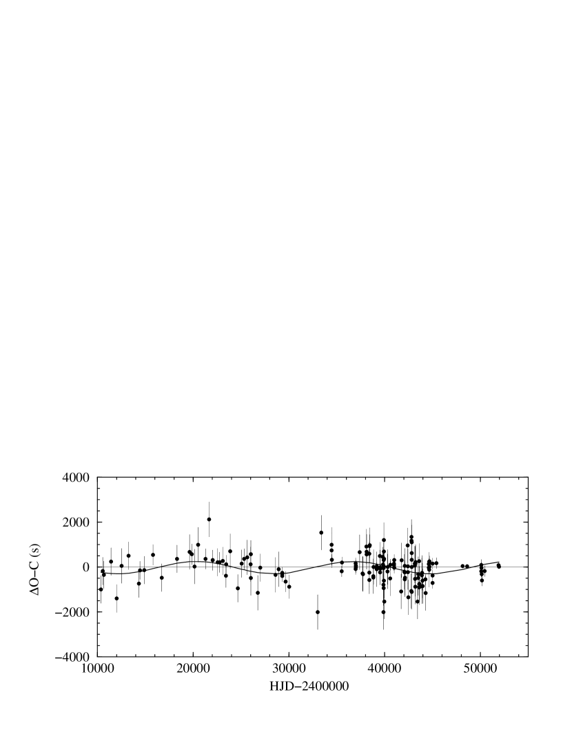
Figure 2.— Residuals of the fit to the LTT orbit of the third body. The remaining oscillations have tentatively been modeled with an LTT perturbation caused by a fourth body in a circular orbit. See text for fit parameters.

Figure 3.— Scale projection on the plane of the sky of the orbits of the eclipsing pair of R CMa (small ellipse) and the tertiary component (large ellipse). The barycenter of the triple system is marked with a plus sign and the positions of the stars in 2002 are represented as small hollow circles. The inset shows a blowup of the region surrounding the barycenter. The orbital properties and the sky projection were derived from the simultaneous analysis of eclipse timing residuals and Hipparcos astrometry (see §4).

References

- Applegate (1992) Applegate, J. H. 1992, ApJ, 385, 621
- Arenou (2001) Arenou, F. 2001, in École de Goutelas #23, eds. D. Egret, J. -L. Halbwachs, & J. -M. Hameury (Paris: Société Française d’Astronomie et d’Astrophysique), 127
- Bachmann & Hershey (1975) Bachmann, P. J. & Hershey, J. L. 1975, AJ, 80, 836
- Bastian (2000) Bastian, U. 2000, IBVS, 4822
- Bystrov (1991) Bystrov, N. F., Polojentsev, D. D., Potter, H. I., Yagudin, L. I., Zalles, R. F., & Zelaya, J. A. 1991, in IAU Colloq. 127, Reference Systems, ed. J. A. Hughes, C. A. Smith, & G. H. Kaplan (Washington: U.S. Naval Observatory), 216
- Deeg et al. (2000) Deeg, H. J., Doyle, L. R., Kozhevnikov, V. P., Blue, J. E., Martín, E. L., & Schneider, J. 2000, A&A, 358, L5
- Delfosse et al. (2000) Delfosse, X., Forveille, T., Ségransan, D., Beuzit, J.-L., Udry, S., Perrier, C., & Mayor, M. 2000, A&A, 364, 217
- Demircan (2000) Demircan, O. 2000, in Variable Stars as Essential Astrophysical Tools, ed. C. İbanoĝlu (Dordrecht: Kluwer), 615
- Dugan & Wright (1939) Dugan, R. S. & Wright, F. W. 1939, Princeton Contrib., 19, 34
- Edalati et al. (1989) Edalati, M. T., Khalesse, B., & Riazi, N. 1989, Ap&SS, 151, 1
- ESA (1997) ESA 1997, The Hipparcos and Tycho Catalogues, ESA SP-1200
- Fabricius (1993) Fabricius, C. 1993, CDS Inf. Bull., 42, 5
- Galeotti (1970) Galeotti, P.. 1970, Ap&SS, 7, 87
- Guinan (1977) Guinan, E. F. 1977, AJ, 82, 51
- Guinan & Ianna (1983) Guinan, E. F. & Ianna, P. A. 1983, AJ, 88, 126
- Guinan & Ribas (2001) Guinan, E. F. & Ribas, I. 2001, ApJ, 546, L43
- Halbwachs et al. (2000) Halbwachs, J. L., Arenou, F., Mayor, M., Udry, S., & Queloz, D. 2000, A&A, 355, 581
- Hodgkin et al. (2000) Hodgkin, S. T., Oppenheimer, B. R., Hambly, N. C., Jameson, R. F., Smartt, S. J., & Steele, I. A. 2000, Nature, 403, 57
- Irwin (1952) Irwin, J. B. 1952, ApJ, 111, 211
- Jordan (1916) Jordan, F. C. 1916, Allegheny Observ. Publ., 3, 49
- Kitamura (1969) Kitamura, M. 1969, Ap&SS, 3, 163
- Knipe (1963) Knipe, G. F. G. 1963, Rep. Observatory Johannesburg Circ., vol. 7, 122, 21
- Koch (1960) Koch, R. H. 1960, AJ, 65, 326
- McArthur et al. (1994) McArthur, B., Jefferys, W., & McCartney, J. 1994, BAAS, 184, 28.04
- Mkrtichian & Gamarova (2000) Mkrtichian, D. E. & Gamarova, A. Yu. 2000, IBVS, 4836
- Qian (2000a) Qian, S. 2000a, AJ, 119, 901
- Qian (2000b) Qian, S. 2000b, AJ, 119, 3064
- Qian (2001) Qian, S. 2001, AJ, 121, 1614
- Radhakrishnan et al. (1984) Radhakrishnan, K. R., Sarma, M. B. K., & Abhyankar, K. D. 1984, Ap&SS, 99, 229
- Robinson (1967) Robinson, L. J. 1967, IBVS, 180, 1
- Sarma et al. (1996) Sarma, M. B. K., Vivekananda Rao, P., & Abhyankar, K. D. 1996, ApJ, 458, 371
- Sawyer (1887) Sawyer, E. F. 1887, AJ, 7, 119
- Serenelli et al. (2001) Serenelli, A. M., Althaus, L. G., Rohrmann, R. D., & Benvenuto, O. G 2001, MNRAS, 325, 607
- Silvestri et al. (2001) Silvestri, N. M., Oswalt, T. D., Wood, M. A., Smith, J. A., Reid, I. N., & Sion, E. M. 2001, AJ, 121, 503
- Sitterly (1940) Sitterly, B. W. 1940, AJ, 48, 190
- Struve (1950) Struve, O. & Smith, B. 1950, ApJ, 111, 27
- Tomkin (1985) Tomkin, J. 1985, ApJ, 297, 250
- Urban et al. (1998) Urban, S. E., Corbin, T. E., Wycoff, G. L., Martin, J. C., Jackson, E. S., Zacharias, M. I., & Hall, D. M. 1998, AJ, 115, 1212
- Varricatt & Ashok (1999) Varricatt, W. P. & Ashok, N. M. 1999, AJ, 117, 2980
- Wilson & Devinney (1971) Wilson, R.E. & Devinney, E.J. 1971, ApJ, 166, 605
- Wolszczan & Frail (1992) Wolszczan, A. & Frail, D. A. 1992, Nature, 355, 145
- Wood (1946) Wood, F. B. 1946, Princeton Contrib., 21, 31
- Zacharias et al. (1992) Zacharias, N., de Vegt, C., Nicholson, W., & Penston, M. J. 1992, A&A, 254, 397