The BOOMERanG experiment
and the curvature of the Universe

Abstract

We describe the BOOMERanG experiment and its main result, i.e. the measurement of the large scale curvature of the Universe. BOOMERanG is a balloon-borne microwave telescope with sensitive cryogenic detectors. BOOMERanG has measured the angular distribution of the Cosmic Microwave Background on $\sim 3\%$ of the sky, with a resolution of $\sim 10$ arcmin and a sensitivity of $\sim 20\mu K$ per pixel. The resulting image is dominated by hot and cold spots with rms fluctuations $\sim 80\mu K$ and typical size of $\sim 1^{o}$. The detailed angular power spectrum of the image features three peaks and two dips at $\ell=(213^{+10}_{-13}),(541^{+20}_{-32}),(845^{+12}_{-25})$ and $\ell=(416^{+22}_{-12}),(750^{+20}_{-750})$, respectively. Such very characteristic spectrum can be explained assuming that the detected structures are the result of acoustic oscillations in the primeval plasma. In this framework, the measured pattern constrains the density parameter $\Omega$ to be $0.85<\Omega<1.1$ (95% confidence interval). Other cosmological parameters, like the spectral index of initial density fluctuations, the density parameter for baryons, dark matter and dark energy, are detected or constrained by the BOOMERanG measurements and by other recent CMB anisotropy experiments. When combined with other cosmological observations, these results depict a new, consistent, cosmological scenario.

1 Introduction

The almost isotropic Cosmic Microwave Background (CMB) accounts for most of the photons present in our Universe. These photons have been produced in the very early Universe, and were last scattered by free electrons at recombination, about 300000 years after the Big Bang. After that, CMB photons travel basically undisturbed along spacetime geodesics for $\sim$ 15 Gyr, reaching our telescopes redshifted by a factor $\sim 1000$ due to the expansion of the universe.

Thus, when we look to the image of the CMB, we see the result of early processes (e.g. the generation of density perturbations at $t\sim 10^{-30}s$ after the Big Bang, and matter-antimatter annihilations, at $t\sim 10^{-5}$ s), of processes in the plasma era till recombination (e.g. acoustic oscillations of the matter-photons plasma till $t\sim 300000yrs$), and of the large scale geometry of the universe (affecting the geodesics followed by the photons after recombination, from $t\sim 300000yrs$ to $t\sim 15Gyrs$ ). Any small curvature of the Universe and of the geodesics would affect significantly the image of the CMB, magnifying or demagnifying it with respect to the Euclidean case. For this reason experiments mapping the CMB are very sensitive to the curvature of the Universe, which, according to General Relativity, is determined by the average mass-energy density of the Universe $\rho$.

A parametric, general relativistic theory of the anisotropy of the CMB has been fully developed in the last 35 years, based on the main cosmological observations: the isotropic expansion of the Universe, the primordial abundances of light elements, the existence of the CMB and its black-body spectrum, the large scale distribution of Galaxies. Detailed models and codes are available to compute the angular power spectrum of the CMB image given a cosmological model for the generation of density fluctuations in the Universe, and a set of parameters describing the background cosmology [1].

The default model is nowadays the inflationary adiabatic one, where gaussian, adiabatic density fluctuations are generated from quantum fluctuations of a scalar field present in the very early Universe, boosted to cosmological scales by the inflation phase at $E\sim 10^{15}GeV$ [2]. This modification of the standard theory is needed in order to solve several paradoxes intrinsic to the standard Hot Big Bang theory. As we will see below, this theory offers a natural explanation to several cosmological observations, but the ingredients required to fit the data are non trivial, requiring the presence of unobserved ”dark matter” and unknown ”dark energy”.

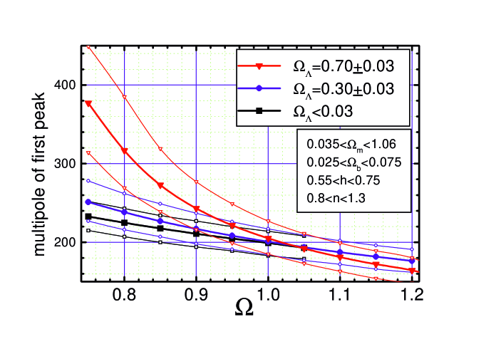
Figure 1: Position of the first peak in the angular power spectrum of the CMB as a function of the total matter-energy density parameter $\Omega$. The results are plotted for a wide database of adiabatic inflationary models ($\sim 5\times 10^{5}$ models corresponding to the ranges of the parameters listed in the bottom panel), for three sample values of $\Omega_{\Lambda}$ (as in the top panel). The thick lines are the average values of $\ell_{1}$. The band within thin lines includes all the possible combinations of the other parameters. See text for details and use of the graph.

The parameters of the model are: the Hubble constant $H_{o}$ (setting the expansion rate of the Universe); the density parameter $\Omega$ (i.e. the ratio between $\rho$ and the critical density $\rho_{c}=3H_{o}^{2}/8\pi G$); the baryons, dark matter and dark energy density parameters $\Omega_{b}$, $\Omega_{m}$, $\Omega_{\Lambda}$; the spectrum of the primordial density fluctuations generating CMB anisotropy. The latter is usually expressed as a power law with spectral index $n$.

The general prediction of the model above is a series of ”acoustic peaks” in the angular power spectrum of the CMB. These peaks derive from acoustic oscillations of the photons-matter plasma (the primeval fireball).

Density perturbations $\Delta\rho/\rho$ were oscillating in the primeval fireball as a result of the opposite effects of the pressure of photons and of gravity. After recombination, photons pressure becomes unimportant, and $\Delta\rho/\rho$ can grow and create, through gravitational instability, the hierarchy of structures we see today in the nearby Universe. There are three physical processes converting the density perturbations present at recombination into observable CMB temperature fluctuations $\Delta T/T$. They are: the photon density fluctuations $\delta_{\gamma}$, which can be related to the matter density fluctuations $\Delta\rho$ once a specific class of perturbations is specified; the gravitational redshift of photons scattered in an over-density or an under-density with gravitational potential difference $\phi_{r}$; the Doppler effect produced by the proper motion with velocity $v$ of the electrons scattering the CMB photons. In formulas:

$$\frac{\Delta T}{T}(\vec{n})\approx\frac{1}{4}\delta_{\gamma r}+\frac{1}{3}{\phi_{r}\over c^{2}}-\vec{n}{\vec{v_{r}}\over c}$$ (1)

where $\vec{n}$ is the line of sight vector and the subscript $r$ labels quantities at recombination.

There is an acoustic horizon at recombination, with a linear size of $\sim 300000$ light-years. At any time $t$ in an infinite Universe regions separated more than $ct$ are not in causal contact. This means that causal horizons, with size $ct$, exist in the Universe. The acoustic horizon has a size similar to the causal horizon, since in the primeval plasma the speed of sound is close to the speed of light. Since the horizon expands with time, any given proper size will eventually become smaller than the acoustic horizon. The time when the proper size of a perturbation becomes equal to the acoustic horizon is called horizon crossing. Perturbations larger than the acoustic horizon at recombination have never been in acoustic contact before, and have not been able to oscillate. Perturbations smaller that that size have oscillated after crossing the horizon, and arrive to recombination with a phase depending on their intrinsic size. The image of the CMB, which is directly observable by means of CMB anisotropy experiments, is a processed image of density perturbations present at recombination. The size of the acoustic horizon is expected to be evident in the size distribution of the detected CMB structures $\Delta T(\alpha,\delta)$. In fact, perturbations with a size close to the acoustic horizon had just enough time to fully compress or rarefy before recombination, and will be evident as cold or hot spots. If we compute the angular power spectrum $c_{\ell}$ of the image, where $c_{\ell}=\langle|a_{\ell,m}|^{2}\rangle$, and $\Delta T(\alpha,\delta)=\sum_{\ell,m}a_{\ell,m}Y^{\ell}_{m}(\alpha,\delta)$, we expect to see a peak corresponding to the angular distance subtended by the acoustic horizon at recombination. In an Euclidean universe, the subtended angle is simply 300000 lyr divided by 15 Glyr and multiplied by a factor 1000, to take into account the subsequent expansion of the Universe. We thus expect structures with a typical angular scale $\theta_{1}\sim 1^{o}$, which corresponds to a multipole $\ell_{1}\sim\pi/\theta_{1}\sim 200$.

This is correct only if the geometry of the Universe is Euclidean, not curved, i.e. if the average mass-energy density of the Universe is the critical one ($\Omega=1$). If, instead, the mass-energy density is higher than critical ($\Omega>1$), the geometry of space will have a positive curvature and the photons will travel along curved geodesics. The excess density will act as a magnifying glass, and the same fluctuations in the CMB will appear as spots larger than $1^{o}$. The opposite will happen if the density is lower than critical, acting as a de-magnifying glass and producing a typical angular size of the fluctuations smaller than $1^{o}$. By measuring the location of the peak it will thus be possible to measure $\Omega$. The quantitative treatment of this angular-size vs distance test can be found in [3], [4]. In general, $\ell_{1}$ decreases when $\Omega$ increases, but the location of the first peak is also controlled by $\Omega_{\Lambda}$, which effectively changes our distance from recombination (see fig.1). Only if $\Omega_{\Lambda}=0$ the simple relationship $\ell_{1}\sim\Omega^{-{1\over 2}}$ holds [3].

CMB experiments are now starting to measure the angular power spectrum with sufficient accuracy to infer $\Omega$ and several other cosmological parameters. This inverse procedure, i.e. measure the cosmological parameters given the observed angular power spectrum and its measurement error, is a complex one, and is further complicated by the presence of degeneracies between the cosmological parameters. Different combinations of the parameters can generate the same power spectrum of the CMB [5], so priors (coming from independent cosmological evidence) must be assumed in the analysis [7]. The measurement of curvature is quite robust in this sense. In fig.1 it is evident that a measurement of e.g. $\ell_{1}=200$ is consistent only with models with $0.85<\Omega<1.1$, for any possible value of the other parameters $\Omega_{\Lambda},\Omega_{b},\Omega_{m},h,n$. More precise measurements of $\Omega$ can be obtained from a full likelihood analysis of the power spectrum data (see below). Once the default model and rather weak priors (for example on the Hubble constant) are assumed, the measurements set very strong constraints also on all the other parameters, and the results are consistent with independent cosmological observations (see e.g. [6]. A new ”precision phase” in the cosmological research seems to be starting. This, however, has a cost, which is the introduction of ”strange” components in the Universe like dark matter and dark energy. Only further observations will show if the latter are just artifices, like Ptolemy’s epicycles deferents and late additions, or, instead, are very important new discoveries.

In this paper we show how the curvature of the Universe has been measured by BOOMERanG. We describe the experiment, then the experimental strategy and observations obtained in the long duration flight, and finally the cosmological implications.

2 The BOOMERanG experiment

2.1 The Observable is small

The CMB is a faint, almost isotropic glow of microwaves. Its purely Planck spectrum has been measured with great accuracy by the COBE-FIRAS experiment [8], [9]. The temperature of the CMB is $T_{o}=2.725K$. Anisotropy in the CMB has been first detected at large angular scales ($>7^{o}$) by the COBE-DMR experiment [10]. At large angular scales the level of the fluctuations detected by COBE-DMR is $\sim$ 10 parts per million of the average level of the CMB: $\Delta T_{rms}\sim 30\mu K$ [11]. This measurement does not allow to measure the curvature of the Universe, since the angular resolution is not enough to resolve the degree-sized hot and cold spots. But it allows us to normalize the angular power spectra computed theoretically, and to predict that the rms of the fluctuations detected with a resolution of, say, 0.2^o, will be in the $100\mu K$ range. This means that a very sensitive microwave telescope is needed. The detection of a sub-degree resolution map of the CMB represents a formidable experimental challenge, since the emissions of the telescope, of the earth atmosphere, of astrophysical foregrounds, and of the isotropic component of the CMB itself, are much higher.

Atmospheric emission is reduced by flying the experiment above the bulk of earth’s atmosphere (38 km), by means of a stratospheric balloon. The observation frequencies of the BOOMERanG experiment (90, 150, 240, 410 GHz) have been carefully selected in order to work in the range where residual atmosphere and galactic foregrounds are minimum. In fig.2 we compare the spectrum of CMB anisotropy to the spectrum of different foregrounds and to the observation frequencies of the BOOMERanG multi-band photometer.

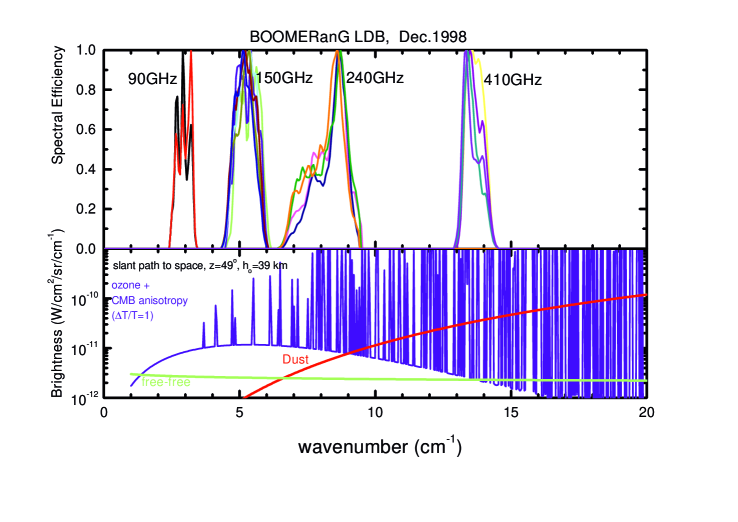
Figure 2: Upper panel: spectral efficiency of all the 16 detection channels of the BOOMERanG experiment. Lower panel: spectrum of the CMB anisotropy, compared to the typical spectra of ozone emission at stratospheric altitudes, of diffuse interstellar dust, of interstellar free-free.

CMB anisotropy brightness has been computed as

$$\Delta I(\nu)={xe^{x}\over e^{x}-1}B(\nu,T_{o}){\Delta T\over T_{o}}$$ (2)

with $x=h\nu/kT_{o}$, where $B(\nu,T_{o})$ is the Planck function, and assuming $\Delta T/T_{o}=1$ in place of $\sim 10^{-4}$. The atmospheric emission at balloon altitude has been computed for a slant path to space with elevation of 41^o, using the HITRAN atmospheric model. Residual water vapor is very low, and oxygen emission is very isotropic. We have included only ozone, which is known to be distributed in stratospheric clouds, and can be potentially dangerous for these measurements [15]. The two bands sensitive to CMB anisotropy are the 90 and 150 GHz ones, which are close to the peak of the CMB anisotropy brightness. The 240 and 410 GHz bands are used to monitor atmospheric and interstellar emission in order to control the level of contamination in the lower frequency maps.

2.2 Experimental approach

The telescope scans the sky in order to separate the anisotropic CMB signal from any isotropic foreground (like instrumental emission) and background (like the isotropic component of the CMB). The signals from the detectors are AC-coupled, so that isotropic emission is rejected. The sky scan is performed at constant elevation. This simple solution strongly reduces the atmospheric signal (only gradients and inhomogeneities contribute, see below).

The azimuth scan speed ${\dot{A}}$ is between 1 and 2 deg/s. Different multipoles $\ell$ in the CMB are converted into different sub-audio frequencies $f$ in the detectors: $f=\ell{\dot{A}}/\pi\cos e$ where $e$ is the elevation of the beam. Multipoles between 20 and 1000 are converted into frequencies $f$ between 0.15-0.3 and 7.5-15 Hz. This range lies inside the flat response band of the detectors, above their 1/f knee frequency, and above the characteristic pendulation frequency of the balloon and payload system.

The payload is flown around Antarctica aboard of a long duration balloon (LDB, $>7$ days) performed by NASA-NSBF. The payload drifts by thousands of km, circumnavigating the Antarctic continent at a nearly constant latitude of -79^o. This enables long integrations, wide sky coverage and extensive tests for systematic effects, through the repetition of the measurements under different experimental conditions. Since the measurements are obtained from different locations we can control spillover from ground, ice and sea. The consistency between maps obtained from different locations is the best test against the presence of sidelobes contributions in the measurements.

The long duration of the flight allows to control the contribution of the sun in the far sidelobes.

”day” (sun at high elevations) vs ”night” (sun at low elevations) observations have different scan directions on the same area, producing nicely cross-linked scans, useful to reconstruct the map of the sky.

We select the lowest foreground sky region for the observations. This happens to be far from the sun in the antarctic summer (constellations of Caelum, Doradus, Pictor, Columba, Puppis). Performing 60^o wide azimuth scans, and tracking the azimuth of the center of the best sky region with the center of the scan, we can cover the best $\sim 4\%$ of the sky in one full day of observation, and repeat the measurement for many days.

2.3 Detection technique

At these frequencies the most sensitive detectors for continuum radiation are cryogenic bolometers. A bolometer consists of a broadband absorber with heat capacity, C, that has a weak thermal link, G, to a thermal bath at a temperature, T_b. Incident radiation produces a temperature rise in the absorber that is read out with a current biased thermistor. The sensitivity of a bolometer expressed in Noise Equivalent Power (NEP) is given by:

$${\rm NEP_{bolo}}=\gamma\sqrt{4k{\rm T_{b}}^{2}{\rm G}}$$ (3)

where $\gamma$ is a constant of order unity that depends weakly on the sensitivity of the thermistor. The need for a cryogenic temperature of the bolometer is evident. Bolometers have been operated at temperatures as low as 0.05 K. The dynamical equation for the temperature of the thermistor can be expressed as:

$$\frac{\rm dT_{bolo}}{\rm dt}=\frac{\rm P_{in}-G(T_{bolo}-T_{b})}{\rm C}$$ (4)

From this equation it is evident that incident background power is equivalent to physical temperature of the device: both need to be as low as possible to get the best NEP. In this respect, balloon-borne experiments allow to achieve a very low background power on the detectors, with the contributions from the CMB, the residual atmosphere and the thermal emission of the optical system are similar. From the same equation we can see that bolometers have a finite bandwidth, limited by the time for the absorber to come to equilibrium after a change in incident power, $\tau=$ C/G. Previous balloon-borne bolometric receivers have been limited in sensitivity or bandwidth by the properties of the materials used for fabrication of the detectors.

Bolometers are also limited in sensitivity by external sources of noise such as cosmic rays, microphonic disturbances, and radio frequency interference (RFI). Of particular importance for BOOMERanG is the cosmic ray rate from balloon altitude in the Antarctic, which is about an order of magnitude higher than from temperate latitudes, because the magnetic field of the earth funnels charged particles to the poles.

The new technology of composite bolometers with metallized Si₃N₄ spider-web absorbers and Ge thermistors [12, 13] has produced bolometers with NEP as low as $2\times 10^{-17}W/\sqrt{Hz}$ at a physical temperature of the device of 300 mK. These bolometers have lower heat capacity, lower thermal conductivities, lower cosmic ray cross section, and less sensitivity to microphonic heating than previous 300 mK bolometers. They also feature very low 1/f noise, with a knee frequency below 0.01 Hz. Spider web bolometers optimized for 100 mK operation and have been recently selected for the HFI instrument on ESA’s CMB mission Planck, which uses a scan strategy similar to BOOMERanG.

The BOOMERanG detectors are optimized to have the maximum sensitivity possible under the estimated loading conditions during the stratospheric flight. The achieved in-flight sensitivities are reported in table 1.

Most bolometric detectors in use today employ a high-impedance semiconductor thermistor biased with a constant current. JFET preamplifiers have been used to provide a combination of low voltage and current noise well matched to typical bolometer impedances, but exhibit excess voltage noise at frequencies typically below a few Hz and have limited the achievable bandwidth of these DC biased bolometers. At lower frequencies, drifts in the bias current, drifts in the temperature of the heat sink, and amplifier gain fluctuations have been expected to limit the ultimate stability of single bolometer systems.

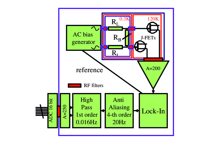
Figure 3: Block diagram of the readout electronics for BOOMERanG. The system is fully differential. Each bolometer is biased through symmetrical smoothed square-waves at a frequency $\sim 300Hz$, higher than its thermal high frequency cut-off. The signal is readout through a differential JFET follower at 120K, located inside the cryostat close to the bolometers. The signal is then amplified and demodulated through a synchronous demodulator locked to the bias frequency. Anti-alias low pass (20 Hz) and background removal high-pass (16 mHz) filtering are then applied. The total amplification is $5\times 10^{4}$. The amplified signal exit the RF-enclosure through RFI filters before A-D conversion (16 bit, 62.5 Hz). 20 identical channels are used for the optical, blank and temperature sensors.

AC bridge circuits have been successfully used to read out pairs of bolometers with DC stability to 30 mHz [14]. In this scheme a pair of detectors is biased with an alternating current so that resistance fluctuations are transformed into changes in the AC bias amplitude across each detector. These signals are differenced in a bridge, amplified and demodulated. The AC signal modulation eliminates the effects of 1/f noise in the preamplifiers since the resulting signal spectrum is centered about the carrier frequency. The effects of drifts in the bias amplitude, amplifier gain, and heat sink temperature are greatly reduced if the two detectors in the bridge are well matched. The optical responsivity of each the detectors in the bridge is equivalent to that of a detector biased with the same rms DC power and is constant in time as long as the average power on the detector is constant over the course of one detector thermal time constant.

For BOOMERanG the environmental background and the refrigerator temperature $T_{b}$ are very stable, so we can employ an AC stabilized ”total power” readout system for individual bolometers [16]. This system contains a cooled FET input stage and contributes less than 10 nV_rms/$\sqrt{\rm Hz}$ noise at all frequencies within the bolometer signal bandwidth down to 20mHz. The warm readout circuit has a gain stability of $<10$ ppm/^∘C , and we remove the large offset due to the background power on the detector with a final stage high pass filter with a cutoff frequency of 16 mHz. A block diagram of the readout system is shown in fig.3.

There are many sources of RFI on the balloon that could couple to bolometers. Microwave transmitters that send the data stream to the ground and high current wires that drive the motors of the Attitude Control System (ACS) are situated within a few meters of the cryostat. The BOOMERANG wiring and focal plane are designed to prevent RF interference from contributing to the noise of the bolometers.

The bolometers are contained inside a 2 K Faraday cage inside the cryostat. RFI can enter the cryostat through the optical entrance window and propagate into the 2 K optics box. However, the exit aperture of the optics box is RF sealed by the horn positioning plate. This plate contains feed horns with small waveguide apertures for radiation from the sky to pass through to the detectors. The largest waveguide feedthrough in this plate is 0.2” in diameter which corresponds to a waveguide cutoff of 40 GHz. Lower frequency RFI is reflected by this surface. Readout wires entering the bolometer Faraday cage can also propagate RF signals as coaxial cables. We run all of the bolometer wires through cast ecosorb filters mounted to the wall of the Faraday cage to attenuate these signals. The filters are 30 cm long and have a measured attenuation of ¡-20 dB at frequencies from 20 MHz to a few GHz.

The readout electronics are also sensitive to RFI. We enclose all of the cryostat electronics in an RF tight box that forms an extension of the outer shell of the cryostat. The signals from the detectors pass through flexible KF-40 hose that is RF sealed to the hermetic connector flange on the cryostat and to the wall of the electronics box. The amplified signals exit the electronics box through MuRata Erie RF filters mounted on the wall of the box. We tested the RF sensitivity of the detectors with a RF sweep generator covering the range 0.1-3 GHz.

2.4 Optics

The sub-degree angular resolution is obtained coupling the bolometers feeds to an off-axis millimeter waves telescope enclosed in a low emissivity cavity. A sketch of the optics is shown in fig.4.

Figure 4: Optical system for BOOMERanG (see text).

The BOOMERanG telescope consists of an ambient temperature 1.2 m off-axis paraboloidal primary mirror which feeds a pair of cold reimaging mirrors inside a large LHe cryostat. The primary mirror has a $45^{\circ}$ off- axis angle and can be tipped in elevation by $+20^{\circ}$ and $-12^{\circ}$ to cover elevation angles from $33^{\circ}$ to $65^{\circ}$. Radiation from the sky is reflected by the primary mirror and passes into the cryostat through a thin (0.002”) polypropylene window near the prime focus. The window is divided in two circles side by side, each 2.6” in diameter. This geometry provides a wide field of view while allowing the use of thin window material which minimizes the emission from this ambient temperature surface. Filters rejecting high frequency radiation are mounted on the 77 K and 2 K shields in front of the cold reimaging optics. Fast off-axis secondary and tertiary mirrors surrounded by black baffles reimage the prime focus onto a detector focal plane with diffraction limited performance at 1 mm over a $2^{\circ}\times 5^{\circ}$ field of view. The reimaging optics are also configured to form an image of the primary mirror at the 10 cm diameter tertiary mirror. The size of the tertiary mirror therefore limits the illumination pattern on the primary mirror which is underfilled by 50% in area.

The BOOMERANG cold optics box shown in Fig.4 contains two paraboloidal mirrors with effective focal lengths of 20 cm and 33 cm for the secondary and tertiary mirrors respectively. The parameters of these mirrors have been optimized for the required performance with CodeV software. The input f/# from the primary mirror is f/2, so the focal plane is fed at f/3.3. The tertiary mirror is 10 cm in diameter, corresponding to an 85 cm diameter aperture on the 1.2 m diameter primary mirror. All of the beams overlap on the primary mirror by $>85$%. The large size of all of the apertures in the system minimizes the effects of diffraction.

The BOOMERANG optics are optimized for an array with widely separated pixels. The advantage of having large spacing between pixels in the focal plane is the ability to difference the signals from two such pixels and remove correlated optical fluctuations such as temperature drift of the telescope, while retaining high sensitivity to structure on the sky at angles up to the pixel separation. This scheme eliminates the need for moving optical components and simplifies the design and operation of the experiment.

The BOOMERANG focal plane contains a combination of single frequency channels fed by conical horns and multicolor photometers fed by winston horns. Although the image quality from the optics is diffraction limited over a $2^{\circ}\times 5^{\circ}$ field, all of the feed optics are placed inside two circles $2^{\circ}$ in diameter, separated center to center by $3.5^{\circ}$. The focal plane area outside these circles is vignetted by blocking filters at the entrance to the optics box and on the 77 K shield and is unusable. Due to the curvature of the focal plane, the horns are placed at the positions of the beam centroids determined from geometric ray tracing. All of the feeds are oriented towards the center of the tertiary mirror.

The projection on the sky of the BOOMERanG focal plane is shown in fig.5.

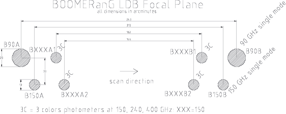
Figure 5: Projection on the sky of the BOOMERanG focal plane. All the measurements are in arcminutes. The two larger beams are for the single-mode 90GHz detectors, while the two detectors immediately below are single-mode 150GHz detectors. The beams A1..B2 are for the four multiband photometers, each observing simultaneously at 150, 240 and 410 GHz. Slow azimuth scans ($\pm 30^{o}$, 1${}^{o}/s$ or 2${}^{o}/s$) are continuously performed at constant elevation, while the center of the scan tracks the azimuth of the lowest foreground region. A structure detected in the forward scan in A1 will be detected a few seconds later in B1, and 30 seconds later in time reverse in B1 and A1 during the return scan. Due to sky rotation, the same sequence of events will be detected a few minutes later in A2 and B2. Hours later, the same sky pixel is observed again with a different inclination of the scan path. All this is repeated every day for 10 days.

The focal plane has been mapped from ground using a far-field spherical black-body, and confirmed in flight through observations of the compact HII region RCW38. The FWHM of the optical system beams is $(18\pm 2)^{\prime}$ at 90GHz, $(10\pm 1)^{\prime}$ at 150GHz, $(14\pm 1)^{\prime}$ at 240 GHz, and $(13\pm 1)^{\prime}$ at 410GHz. The effective beam during the observations is obtained convolving the optical beam with the pointing jitter, which is of the order of 2.5’ rms in the current pointing solution.

2.5 Cryogenics

The bolometers and the reimaging optics are cooled by a combination of a large L⁴He/LN cryostat and a high capacity ³He fridge. The long hold time (2 weeks) has been obtained using a 20K vapor cooled shield for the liquid He tank and superinsulation for the nitrogen tank. The tanks are supported by kevlar cords. The details of the main cryostat are reported in [17]. The details of the ³He fridge are reported in [18]. The cryogenic system performed well, keeping the detectors well below their required operating temperature of 0.3 K for the entire flight. A small daily oscillation of the main helium bath temperature was induced by daily fluctuations of the external pressure. In fact, the altitude of the payload varies with the elevation of the sun, which oscillates between 11^∘ to 35^∘ diurnally. We have searched for scan synchronous temperature fluctuations in the ³He evaporator and in the ⁴He temperature, and we find upper limits of the order of 1 $\mu K_{rms}$ during the 1^∘/s scans, and drifts with an amplitude of a few $\mu K$ during the 2^∘/s scans.

2.6 The payload

A sketch of the payload is reported in fig.6. The total weight of the science payload is $\sim$ 1.5 tons. There is one inner frame supporting the telescope and the cryostat with the detection system. The inner frame can tilt with respect to the outer frame, in order to point the telescope at different elevations. The outer frame supports the attitude control system (ACS), data storage and telemetry electronics.

The ACS must be able to point a selected sky direction, and track it or scan over it with a reasonable speed. The specifications are 1 arcmin rms for pointing stability, with a reconstruction capability better than 0.5 arcmin. The BOOMERANG ACS is based on a pivot which decouples the payload from the flight chain and controls the azimuth, plus one linear actuator controlling the elevation of the inner frame of the payload. The pivot has two flywheels, moved by powerful torque motors with tachometers. On the inner frame, which is steerable with respect to the gondola frame, are mounted both the telescope and the cryogenic receiver. The observable elevation range is between 33 and 65 deg. The attitude sensors are a low and a high resolution sun sensor and a set of laser gyroscopes (3-axis). A differential GPS is also used as an absolute attitude reconstruction system. A flight programmer CPU takes care of commands handling and observations sequencing; a feedback loop controller CPU is used for digitization of sensors data and PWM control of the current of the three torque motors.

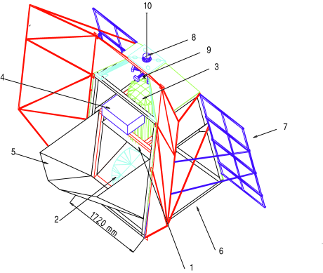
Figure 6: The BOOMERanG payload. On the inner frame (1) are mounted the off axis primary mirror (2), the cryostat with the detection system (3), the analog electronics (4), the ground shield (5). On the outer frame (6) are mounted the sun shields, the solar panels (7), the azimuth pivot (8) with the flywheel (9). The pivot decouples the payload from the flight chain (10).

3 The LDB flight and the maps of the microwave-sky

BOOMERanG was launched from McMurdo Station (Antarctica) on 29 December 1998, at 3:30 GMT. Observations began 3 hours later, and continued uninterrupted during the 259-hour flight. The payload approximately followed the 79^∘ S parallel at an altitude that varied daily between 37 and 38.5 km, returning within 50 km of the launch site. The time-ordered data (TOD) comprises $5.4\times 10^{7}$ 16-bit samples for each channel. These data are flagged for cosmic-ray events, elevation changes, focal-plane temperature instabilities, and electromagnetic interference events. In general, about 5% of the data for each channel are flagged and not used in the subsequent analysis. The gaps resulting from this editing are filled with a constrained realization of noise in order to minimize their effect in the subsequent filtering of the data. The data are deconvolved by the bolometer and electronics transfer functions to recover uniform gain at all frequencies; a high pass filter with null response at $f=0$ and unit response at $f=0.01Hz$ has been applied to remove low frequency drifts and system instabilities. The pointing of the telescope has been reconstructed for each data in the TOD combining the signals of the gyroscopes, of the sun sensors and of the differential GPS. A time ordered pointing (TOP) dataset has been created for each pixel in the focal plane.

The gain calibrations are obtained from observations of the CMB dipole. To compare with the data, we artificially sample the CMB dipole signal [24], corrected for the Earth’s velocity around the sun [25], according to the BOOMERANG scanning, and filter this fake time stream in the same way as the data. The 1 dps data is then fit simultaneously to this filtered dipole, a similarly filtered dust emission model [26], an offset and the BOOMERANG 410 GHz data for all data more than 20 degrees below the Galactic plane. The dipole calibration numbers obtained with this fit are robust to changes in Galactic cut, and to whether or not a dust model is included in the fit; this indicates that dust is not a serious problem for the contamination. They are insensitive to the inclusion of a 410 GHz channel in the fit, which is a general indication that there is no problem with a wide range of systematics such as atmospheric contamination, as these would be traced by the 410 GHz data. The gain calibration accuracy is estimated to be $\sim 10\%$, with the error dominated by systematics.

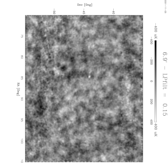
Figure 7: Map of the microwave sky measured by BOOMERanG at 150 GHz. The effective resolution of the observations is 12 arcmin. Healpix pixelization with 3.5’ pixel side has been used. The map has been convolved with a 9’ FWHM gaussian kernel for visualization purposes. The units correspond to thermodynamic temperature fluctuations of a 2.73K blackbody. The same structures are visible in the 90 GHz and in the 240 GHz maps of BOOMERanG.

Several independent methods have been used to estimate the map of the observed sky region from the TOD and TOP: Naive maps (just coadding data on the same pixel); maximum likelihood maps obtained using the MADCAP package ([38]); maximum likelihood maps obtained using the iterative method of [20]; suboptimal maps obtained using the fast map making method of [21]. All methods produce very similar maps. In fig.7 we show the central region of the 150GHz map from the B150A channel obtained with the iterative method [20]. The color code used in the BOOMERanG maps corresponds to temperature fluctuations of a 2.73K blackbody. Degree-scale structures with amplitude of the order of 100 $\mu K$ are evident in the map at 150 GHz. Consistent structure is also evident in the maps at 90 and 240 GHz. The similarity of the temperature maps obtained at different frequencies [22] is the best evidence for the CMB origin of the detected fluctuations.

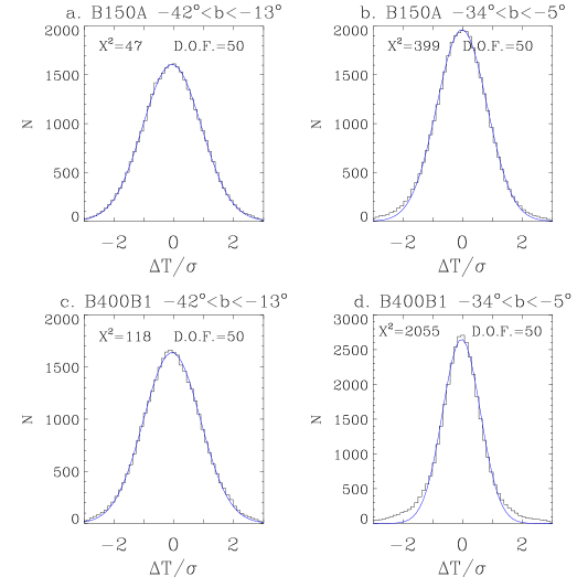
Figure 8: In the top row, we plot the 1-P distribution of the ratio $\Delta T_{i}/\sqrt{\sigma_{i}^{2}+\sigma_{sky}^{2}}$ for the 150 GHz map (dominated by CMB fluctuations) in a box at high galactic latitude (a) and in a box at intermediate galactic latitudes (b). In the lower row the same distributions are plotted for the map at 410 GHz, which is dominated by interstellar dust

Foregrounds contamination can be constrained significantly in the center of the observed sky region [22], [23]. In fact, in the frequency region of interest, the most important foregrounds are thermal emission from interstellar dust and unresolved extragalactic sources. Galactic synchrotron and free-free emission is negligible at this frequency[27]. Contamination from extra-galactic point sources is also small [28]; extrapolation of fluxes from the PMN survey [29] limits the contribution by point sources (including the three above-mentioned radio-bright sources) to the angular power spectrum derived below to $<0.7\%$ at $\ell=200$ and $<20\%$ at $\ell=600$. Masi et al. [23] have shown that thermal emission from interstellar dust, as mapped by the IRAS satellite at 3000 GHz, is strongly correlated to the emission dominating the BOOMERanG map at 410 GHz. The slope of a linear fit of the BOOMERanG data vs the IRAS data is $S=(4700\pm 1500)\mu K_{CMB}/(MJy/sr)$; Pearson’s linear correlation coefficient is R=0.138 with 68987 data (pixels) at Galactic latitudes lower than -20^o. At this frequency, CMB anisotropy is subdominant and barely detected in the BOOMERanG maps. On the other hand, the lower frequency maps of BOOMERanG, where CMB anisotropy is dominant, are much less correlated: the slopes are $S=(258\pm 52)\mu K_{CMB}/(MJy/sr)$ with R=0.041; $S=(46\pm 29)\mu K_{CMB}/(MJy/sr)$ with R=0.003; $S=(-20\pm 110)\mu K_{CMB}/(MJy/sr)$ with R=-0.028 at 240, 150 and 90 GHz respectively. Using these data, it has been shown that the mean square signal due to interstellar dust at 150 GHz is about two orders of magnitude smaller than the CMB anisotropy. The residuals of the correlation give upper limits of the same order of magnitude for any other dust component (not correlated to the emission mapped by IRAS).

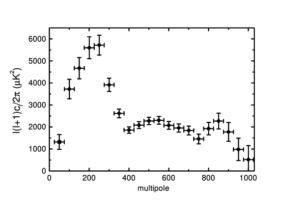
Figure 9: CMB anisotropy power spectrum detected by BOOMERanG at 150 GHz. The circles are from the Monte-Carlo approach, while the point at $\ell=50$ is from the rigorous maximum likelihood approach. Only statistical errors (instrumental and cosmic/sample variance) are shown. The gain calibration error is 10% (i.e. 20% in the power spectrum), while the beam calibration error is 1.4’ in the FWHM, and affects (in a coherent way) the highest multipoles.

4 Gaussianity

According to the currently popular inflation scenario one important property of the CMB anisotropy is its gaussianity. This makes the CMB very special, since any other astrophysical source produces strongly non-gaussian patterns in the sky. If the CMB is really gaussian, all its statistical properties are encoded in its angular power spectrum. At large scales, gaussianity of the CMB has been investigated and confirmed using the COBE maps [30, 31, 32, 33]. At smaller scales, where the natural tendency to gaussianity due to the central limit theorem is less effective, the CMB has been found to be fully gaussian by the QMASK [34] and MAXIMA [35, 36] experiments. Due to its wide sky and frequency coverage, BOOMERanG is ideally suited to carry out an accurate analysis of the possible systematic effects present in the detected signal. This issue is studied in detail in [37], who use five estimators of departures from gaussianity: the skewness and kurtosis of the CMB temperature distribution, and the three Minkowski functionals of the maps: area, length and genus. All these methods confirm the gaussianity of the CMB fluctuations detected by BOOMERanG. In fig.8 we plot the simple 1-point distribution of the data: the gaussianity of the CMB dominated high latitude 150 GHz map is evident, while the sky is not gaussian at lower latitudes and at 410 GHz (where emission is contaminated or dominated by interstellar dust and detector noise).

5 The Power spectrum

We have computed the power spectrum of the 150 GHz maps detected by BOOMERanG with two independent methods: the rigorous (and computationally expensive) maximum likelihood approach of [38], and the Monte-Carlo approach of [39]. Both methods give consistent results. The best estimate of the power spectrum from BOOMERanG at 150 GHz is shown in fig.9, where we have combined the results of the Monte Carlo method of [40] at $\ell>75$ with the lowest bin of the maximum likelihood spectrum of [22], corrected for the improved calibration. In fig.10 we compare the BOOMERanG power spectrum at 150 GHz to the spectra measured by the experiments DASI (at 30 GHz)[41] and MAXIMA (at 150 GHz) [42]. Despite of the orthogonal experimental techniques and different observed regions, the three results are statistically consistent.

Netterfield et al. [40] have discussed how the measured power spectrum of the sky is robust against variations of the $\ell$-binning, channel selection, data subset selection, effects of uncertainties in the beam and effects of the noise. de Bernardis et al. [43] have shown that the three peaks and two dips present in the power spectrum are statistically significant. The first peak is at $\ell_{1}=(213^{+10}_{-13})$ (the errors correspond to a 1$\sigma$ confidence interval in the location if the peak). Its amplitude is detected at $\lower 2.15277pt\hbox{$\;\buildrel>\over{\sim}\;$}5\sigma$, while for the second peak (at $\ell_{2}=(541^{+20}_{-32})$) and third peak (at $\ell_{3}=(845^{+12}_{-25})$) the amplitudes are detected at basically 2$\sigma$. Several methods to measure the location and amplitude of the peaks have been compared, all producing very consistent results. In particular, the results of fits using empirical functions are consistent with the results of fits using a database of adiabatic inflationary spectra of the CMB [43].

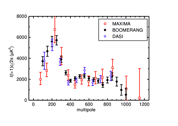
Figure 10: CMB anisotropy power spectrum detected by BOOMERanG, MAXIMA and DASI. Approximately uncorrelated band-powers are plotted for each of the experiments. The error bars represent statistical errors only.

6 Cosmological implications

The measurement of $\ell_{1}$ from the most recent BOOMERanG power spectrum is $\ell_{1}=(213^{+10}_{-13})$, which is consistent with a flat geometry of the Universe. Rigorous confidence intervals for the parameter $\Omega$ can be found with the Bayesian analysis of the full power spectrum, as described below. These methods use the full information content of the data (and not just the location of the peak) and take in due account the degeneracies between different parameters.

The ratio between the amplitude of the second peak and the amplitude of the first one depends mainly on the physical density of baryons $\Omega_{b}h^{2}$ and on the tilt of the density fluctuations spectrum. A high density of baryons favors compressions against rarefactions: the odd-order peaks (compression) are enhanced while the even-order peaks (rarefaction) are depleted. From the BOOMERanG power spectrum the ratio is $(5450\pm 350)/(2220\pm 330)=(2.45\pm 0.52)$. Assuming a scale invariant power spectrum of the density fluctuations ($n=1$), this corresponds to a physical density $\Omega_{b}h^{2}\sim 0.02$. Again, better constraints are found by means of the Bayesian analysis of the full power spectrum as described below. In fact, a tilt of the density fluctuations spectrum ($n<1$) has the same effect of a high baryons density in depleting the second peak with respect to the first one, so there is a degeneracy between the two parameters. But the effects of the two quantities on the amplitude of the third peak are different. The amplitude of the third peak is increased by a high baryon density, while it is decreased by a red ($n<1$) primordial density fluctuation spectrum. The result is that extending the observations to $\ell\sim 1000$ breaks the degeneracy between $n$ and $\Omega_{b}h^{2}$, thus allowing a determination of both the parameters.

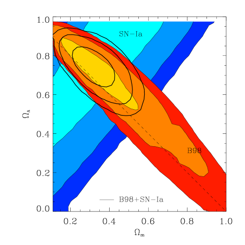
Figure 11: Constraints in the $\Omega_{m}$ vs. $\Omega_{\Lambda}$ plane from the combined BOOMERANG and COBE/DMR datasets, assuming the weak prior $0.45<h<0.85$, and an age of the Universe $>10$ Gyr. The likelihood at each point is calculated by maximizing over the remaining cosmological parameters. The shaded regions correspond to the $68.3\%$, $95.4\%$ and $99.7\%$ confidence levels. The CMB contours (labeled B98) are overlaid on the contours derived from observations of high redshift supernovae (labeled SN 1a). The line contours are for the combined likelihood.

It is important to stress the fact that our result for $\Omega_{b}h^{2}$ agrees with the constraint on $\Omega_{b}h^{2}$ from the Big Bang Nucleosynthesis. In fact, the physical density of baryons affects the yield of the nuclear reactions happening in the first few minutes after the big bang. The resulting primordial abundances of light elements are measured by the optical absorption spectra of primordial clouds of matter [44]. It is evident that both the physics and the experimental methods involved in these two measurements of $\Omega_{b}h^{2}$ are completely orthogonal to the CMB ones. The fact that the two estimates of $\Omega_{b}h^{2}$ agree so well should be considered a great success of the Hot Big Bang model.

The multiple peaks and dips are a strong prediction of the simplest adiabatic inflationary models, and more generally of models with passive, coherent perturbations. Although the main effect giving rise to them is regular sound compression and rarefaction of the photon-baryon plasma at photon decoupling, there are a number of influences that make the regularity only roughly true. The best way to extract all the information encoded in the data is by comparison to a large database of $C_{\ell}$ spectra. In order to limit the size of the database, we considered for the first approach the class of adiabatic inflationary models. We have explored a parameter space with 6 discrete parameters and a continuous one. The parameters ranged as follows: $\Omega_{m}=0.11,...,1.085$, in steps of 0.025; $\Omega_{b}=0.015,...,0.20$, in steps of 0.015; $\Omega_{\Lambda}=0.0,...,0.975$, in steps of 0.025; $h=0.25,...,0.95$, in steps of 0.05; spectral index of the primordial density perturbations $n_{s}=0.50,...,1.50$, in steps of 0.02, $\tau_{C}=0.,..,0.5$, in steps of 0.1. The overall amplitude $C_{10}$, expressed in units of $C_{10}^{COBE}$, is allowed to vary continuously. We used the BOOMERANG power spectrum expressed as $18$ bandpowers $C_{b}$ [40] and we computed the likelihood for the cosmological model $C_{b}^{T}$ as $\exp(-\chi^{2}/2)$, where $\chi^{2}=(C_{b}-C_{b}^{T})M^{-1}_{bb^{\prime}}(C_{b^{\prime}}-C_{b^{\prime}}^{T})$. Here $M_{bb^{\prime}}$ is the covariance matrix of the measured bandpowers; $C_{b}^{T}$ is an appropriate band average of $C_{\ell}$. A $10\%$ Gaussian-distributed calibration error in the gain and a 1.4’ (13%) beam uncertainty were included in the analysis as additional parameters with gaussian priors. The COBE-DMR bandpowers used were those of [45], obtained from the RADPACK distribution [46]. The 95% confidence intervals for the parameters we find in this way depend to some extent on the priors assumed. Using COBE and BOOMERanG data only, with a weak prior $0.45<h<0.9$ significantly constrains three parameters: $0.9<\Omega<1.15$, $0.8<n<1.1$ and $0.015<\Omega_{b}h^{2}<0.029$.

The detailed breakdown of $\Omega$ in $\Omega_{m}$ and $\Omega_{\Lambda}$ cannot be inferred by CMB data alone. In fig.11 we plot the joint likelihood for $\Omega_{m}$ and $\Omega_{\Lambda}$ using the BOOMERanG and COBE data, and the weak prior $0.45<h<0.85$ and an age of the Universe $>$ 10 Gyrs.

Using more restrictive priors, deriving from the properties of the large scale distribution of Galaxies ($\sigma_{8}$ and $\Gamma$), or the data of high-redshift supernovae, or the measurement of $h$ by the HST, produces narrower, consistent intervals for all the parameters [40], [43]. This fact suggests a good overall consistency of the present cosmological paradigm. Including these priors, it is also possible to constrain the two additional forms of mass-energy contributing to the total mass-energy density in the Universe, i.e. dark matter and dark energy. We find that the 95% confidence intervals for $\Omega_{m}h^{2}$ and $\Omega_{\Lambda}$ are $0.36<\Omega_{\Lambda}<0.72$ and $0.09<\Omega_{m}h^{2}<0.18$ (LSS prior); $0.52<\Omega_{\Lambda}<0.88$ and $0.01<\Omega_{m}h^{2}<0.17$ (SN1a prior); $0.40<\Omega_{\Lambda}<0.84$ and $0.06<\Omega_{m}h^{2}<0.26$ (HST $h$ prior). The detection of a non-zero $\Omega_{\Lambda}$ comes thus from independent paths and sets a formidable challenge to our understanding of fundamental physics [47].

7 Conclusions

The BOOMERanG experiment has produced multi-frequency maps of the microwave sky, where the structure of the CMB has been resolved with high signal to noise ratio. The structures in the CMB are gaussian, and their power spectrum features three peaks. This is consistent with the presence of acoustic oscillations in the primeval plasma. It also fits the predictions of the adiabatic inflationary scenario. The values of the cosmological parameters inferred in this scenario point to a flat universe (the 95% confidence interval is $0.85<\Omega<1.1$) with nearly scale-invariant initial adiabatic perturbations and a significant contribution of dark energy to the total density of the Universe. These results from BOOMERanG have been confirmed by independent CMB experiments (like DASI and MAXIMA) and by other cosmological observations. The forthcoming space missions MAP and Planck will improve significantly the precision of these results, either entering the ”precision cosmology” era, or detecting hidden inconsistencies of the present cosmological scenario.

References

- [1] Hu W., and Dodelson A., Ann.Rev.Astron.Astrophys., astro-ph/0110414, (2002).
- [2] E.W. Kolb and Turner M.S, The Early Universe, Addison-Wesley, (1990).
- [3] Weinberg S., Phys.Rev. D62, 127302, (2000)
- [4] Melchiorri A. and Griffiths L.M., astro-ph/0011147, (2000)
- [5] see e.g. Efstathiou G., and Bond, J. R., MNRAS, 304, 75, (1999).
- [6] see e.g. Wang X., et al., astro-ph/0105091 (2002).
- [7] see e.g. Lange A.E., et al., Phys. Rev. D 63, 042001 (2001).
- [8] Mather J., et al., Ap.J., 354, L37, (1990).
- [9] Mather J., et al., Ap.J., 512, 511, (1999).
- [10] Smoot G., et al., Ap.J., 396, L1, (1992)
- [11] Banday A., et al., (1996), astro-ph/9601065
- [12] Mauskopf P. et al., Applied Optics 36, 765-771, (1997)
- [13] Bock J., et al., Proc. SPIE 3357, 297-304, (1998) Advanced Technology MMW, Radio, and Terahertz Telescopes, T.G. Phillips Ed.
- [14] Wilbanks, T., et al. IEEE Trans. Nucl. Sci., 37, 566, (1990)
- [15] Page L.A., et al., Ap.J., 355, L1, (1990)
- [16] Hristov V.V. et al., in preparation (2002).
- [17] Masi S., et al., Cryogenics, 39, 217-224 (1999).
- [18] Masi S., et al., Cryogenics, 38, 319-324 (1998).
- [19] Borrill, J., in 3K Cosmology astro-ph/9911389
- [20] Natoli P., et al. 2001, submitted to Ap.J., astro-ph/0101252
- [21] Hivon E. et al., 2001, submitted to Ap.J., astro-ph/0105302
- [22] de Bernardis, P., et al. Nature, 404, 955, (2000).
- [23] Masi S., et al., Ap.J, 553, L93-L96, (2001).
- [24] Lineweaver, C.H., et al., Ap.J., 470, 38, (1996).
- [25] Stumpff, A&A Suppl., 41, 1, (1980).
- [26] Finkbeiner D.P. et al. Ap.J., 524, 867, (1999).
- [27] Kogut A., in Microwave Foregrounds, Eds. de Oliveira Costa and Tegmark, Astron. Soc. Pacific Conf. Series 181, 91-99, (1999)
- [28] Toffolatti L., et al., MNRAS, 297, 117-127 (1998)
- [29] http://astron.berkeley.edu/wombat/foregrounds/radio.html
- [30] Ferreira P.G. et al., Ap.J., 503, L1, (1998)
- [31] Banday A., et al., Ap.J., 533, 575, (1999)
- [32] Komatsu E., et al., 2001, astro-ph/0107605
- [33] Bromley B.C., and Tegmark M., Ap.J., 524, L79, (2000).
- [34] Park C. et al. 2001, submitted to Ap.J., astro-ph/0102406
- [35] Santos M.G. et al., 2001, astro-ph/0107588
- [36] Wu J.H.P. et al., 2001, astro-ph/0104248
- [37] Polenta G., et al., 2002, submitted to Ap.J.
- [38] Borrill J. 1999, Proc. of the 3K Cosmology EC-TMR conference, eds. L. Maiani, F. Melchiorri, N. Vittorio, AIP CP 476, 277
- [39] Hivon, E. et al. 2001, astro-ph/0105302
- [40] Netterfield C.B., et al. , Ap.J., in press, (2002), astro-ph/0104460
- [41] Halverson N.W. et al. 2001, astro-ph/0104489
- [42] Lee A.T. et al. 2001, astro-ph/0104459
- [43] de Bernardis, P., et al. Ap.J. , in press, (2002), astro-ph/0105296
- [44] Burles, S., Nollett, K.M. & Turner, M.S. 2000, astro-ph/0010171
- [45] Bond, J.R., Jaffe, A.H. & Knox, L. 1998, Phys. Rev. D57, 2117
- [46] Knox L. 2000, http://flight.uchicago.edu/knox/radpack.html
- [47] Weinberg S., Rev. Mod. Phys., 61, 1, (1989).