Measuring the broadband power spectra of active galactic nuclei with RXTE

Abstract

We have developed a Monte Carlo technique to test models for the true power spectra of intermittently sampled lightcurves against the noisy, observed power spectra, and produce a reliable estimate of the goodness of fit of the given model. We apply this technique to constrain the broadband power spectra of a sample of four Seyfert galaxies monitored by the Rossi X-ray Timing Explorer (RXTE) over three years. We show that the power spectra of three of the AGN in our sample (MCG-6-30-15, NGC 5506 and NGC 3516) flatten significantly towards low frequencies, while the power spectrum of NGC 5548 shows no evidence of flattening. We fit two models for the flattening, a ‘knee’ model, analogous to the low-frequency break seen in the power spectra of BHXRBs in the low state (where the power-spectral slope flattens to $\alpha=0$) and a ‘high-frequency break’ model (where the power-spectral slope flattens to $\alpha=1$), analogous to the high-frequency break seen in the high and low-state power spectra of the classic BHXRB Cyg X-1. Both models provide good fits to the power spectra of all four AGN. For both models, the characteristic frequency for flattening is significantly higher in MCG-6-30-15 than in NGC 3516 (by factor $\sim 10$) although both sources have similar X-ray luminosities, suggesting that MCG-6-30-15 has a lower black hole mass and is accreting at a higher rate than NGC 3516. Assuming linear scaling of characteristic frequencies with black hole mass, the high accretion rate implied for MCG-6-30-15 favours the high-frequency break model for this source and further suggests that MCG-6-30-15 and possibly NGC 5506, may be analogues of Cyg X-1 in the high state. Comparison of our model fits with naive fits, where the model is fitted directly to the observed power spectra (with errors estimated from the data), shows that Monte Carlo fitting is essential for reliably constraining the broadband power spectra of AGN lightcurves obtained to date.

1 Introduction

The strong and rapid X-ray variability observed in many Seyfert galaxies on time-scales of a day or less provides strong evidence that the X-rays are emitted close to the central black hole. Early efforts to characterise the X-ray variability, using data from EXOSAT, showed that it has a scale-invariant, red-noise form on time-scales from a few hundred seconds up to the few-days duration of the observations (M^cHardy & Czerny 1987, Lawrence et al. 1987). Later studies of the X-ray variability properties of large samples of radio-quiet AGN showed that the variability amplitude scales inversely with luminosity (Green, M^cHardy & Lehto 1993; Lawrence & Papadakis 1993; Nandra et al. 1997). One possible explanation of this result is that the higher luminosity AGN contain more massive black holes and the variability time-scales in AGN scale with black hole mass. Intriguingly, black hole X-ray binary systems (BHXRBs) also show red-noise type variability of a similar amplitude to AGN, on time-scales less than seconds. The similarity in X-ray variability properties of AGN and BHXRBs raises the possibility that the processes causing variability in AGN and BHXRBs are the same and that any characteristic variability time-scales scale with the central black hole mass. This possibility can be tested by comparing the detailed X-ray timing properties of BHXRBs and AGN.
Timing studies of BHXRBs are usually carried out in the frequency domain using the power spectrum, which shows the contribution of variations on different time-scales (corresponding to power-spectral frequencies) to the total variability of the lightcurve. The power spectra of BHXRBs are dominated by a broadband noise component (van der Klis 1995). On short time-scales, the variability is characterised as scale-invariant ‘red noise’, producing a power-law power spectrum (power $P(\nu)$ at frequency $\nu$ is given by $P(\nu)\propto\nu^{-\alpha}$ where $\alpha$ is the power-spectral slope) of slope $\alpha\sim 1$–$2.5$ (van der Klis 1995). In the ‘low’ state, characterised by a relatively hard X-ray spectrum (similar to that of AGN), the power spectrum flattens towards lower frequencies so that on long time-scales the X-ray lightcurve becomes ‘white noise’, with corresponding slope $\alpha\simeq 0$. For example, in the classic BHXRB system Cyg X-1, the power-spectral flattening is well described by a power-law with two breaks, a high-frequency break which varies between 1 and 6 Hz, above which the power-spectral slope varies between $\alpha\sim 1.5$–$2.4$ and a low-frequency break which varies between 0.04 and 0.4 Hz, above which the power-spectral slope $\alpha\simeq 1$ and below which the slope $\alpha\simeq 0$ (Belloni & Hasinger 1990). In contrast, the power spectrum of the ‘high’ (soft energy spectrum) state seen in some BHXRBs (inluding Cyg X-1) does not flatten to zero slope; instead, the slope $\alpha\simeq 1$ below the high-frequency break extends to $<10^{-2}$ Hz (e.g. Cui et al. 1997).
In order to test the hypothesis that the X-ray variability of AGN is similar to that of BHXRBs over a broad range of time-scales, we must search for low-frequency flattening in the broadband power spectra of AGN. By fitting models with power-spectral breaks to the AGN power spectra and comparing the estimated break frequencies with what we expect if they correspond to similar breaks in BHXRB power spectra, we can test the possibility that the power-spectral shape is really the same and scales simply with black hole mass. If so, we expect break frequencies in AGN to be found at frequencies of $\sim 10^{-5}$ Hz or lower, so that monitoring observations on time-scales of weeks or longer are necessary to detect any flattening in the power spectrum.
Early attempts to measure broadband power spectra of AGN were hampered by the sparseness of long-term archival lightcurves, which had to be constructed from data obtained by several missions (M^cHardy 1988). Nonetheless, some evidence for power-spectral flattening was found, but models for the form of the flattening could not be constrained (Papadakis & M^cHardy 1995).
Ideally, broadband power spectra should be measured from lightcurves obtained with frequent and regular sampling over a long duration, which previous missions were not optimised to do. The Rossi X-ray Timing Explorer (RXTE), which has just such a capability, was launched in December 1995. RXTE carries a large-area proportional counter array (the PCA) which can detect many AGN with good signal-to-noise in less than 1000 s, but most importantly, RXTE can slew rapidly so that it may monitor many targets with frequent 1 ks snapshots.
We have monitored a sample of 4 Seyfert galaxies (MCG-6-30-15, NGC 4051, 5506 and 5548) with RXTE since 1996, in order to measure their broadband power spectra. These objects are known to be significantly X-ray variable and cover a broad range of X-ray luminosity (NGC 4051$\sim 5\times 10^{41}$ erg s^-1, MCG-6-30-15 and NGC 5506$\sim 1.5\times 10^{43}$ erg s^-1, NGC 5548$\sim 5\times 10^{43}$ erg s^-1) and presumably, a broad range of black hole masses. We describe the power spectrum of NGC 4051, which shows unusual non-stationarity in its lightcurve (Uttley et al. 1999) in a separate paper (Papadakis, M^cHardy & Uttley, in prep.). In this paper, we present a power-spectral study of the remaining three objects in our sample using data from RXTE cycles 1, 2 and 3, also including the excellent lightcurves obtained as part of a separate power-spectral study of the Seyfert 1 galaxy NGC 3516 (luminosity$\sim 1.5\times 10^{43}$ erg s^-1), by Edelson & Nandra (1999). We describe data reduction and present the lightcurves in Section 2.
The estimation of the underlying power-spectral shape from lightcurves which are discretely (and possibly unevenly) sampled is hampered by the distorting effects of aliasing and red-noise leak. A further serious problem is that the measured power spectra are intrinsically noisy, and reliable errors on the power in each frequency bin cannot be estimated from the data (especially at low frequencies), due to the small number ($<20$) of power-spectral measurements made in each frequency bin. In Section 3, after presenting the observed power spectra, we describe these problems, which previous efforts to constrain the shape of the broadband power spectrum of AGN using RXTE data (e.g. Edelson & Nandra 1999, Nowak & Chiang 2000) have not accounted for.
To overcome the difficulties in estimating the true power-spectral shape, we have developed a method which we call psresp, based on the response method (Done et al. 1992) which uses Monte Carlo simulations of lightcurves to take account of the distorting effects of sampling and to estimate uncertainties, allowing us to test various power-spectral models against the data. We describe psresp in Section 4, and apply it to the lightcurves of our sample of Seyfert galaxies in Section 5, in order to test for flattening in their broadband power spectra and constrain simple models for describing any flattening we see. In Section 6, we compare our results with those obtained by naively fitting the observed power spectrum (without taking proper account of errors and the distortion due to sampling), use our power spectral measurements to estimate the black hole masses of the AGN in our sample and discuss some of the implications of our results, before making concluding remarks in Section 7.

2 The lightcurves

2.1 Observations and data reduction

We use data obtained with the PCA on board RXTE covering a three year period during observing cycles 1–3 when the PCA gain setting was constant, so that count rate measurements provide a simple measure of observed flux. Of the three instruments on board RXTE, only the PCA is sensitive enough to allow us to make an accurate flux measurement for our targets with the 1 ks snapshots which our monitoring consists of. The PCA consists of 5 Xenon-filled Proportional Counter Units (PCUs), numbered 0 to 4 which are sensitive in the 2–60 keV energy range and contribute to a total effective area of 6500 cm². Since launch, discharge problems have meant that one or both of PCUs 3 and 4 are often switched off (this problem extended to PCU 1 in March 1999 but we do not include this later data here). Despite the loss of up to two PCUs during our observations, we are easily able to obtain sufficient signal-to-noise in a single snapshot for our purposes ($S/N>20\sigma$).

Table 1: Lightcurve details

	Long-term		Intensive		Long-look
	Start	Stop	Start	Stop	Start	Stop	Exp
MCG-6-30-15	8 May 1996	2 Feb 1999	23 Aug 1996	29 Sep 1996	03:31 ut 4 Aug 1997	12:34 ut 12 Aug 1997	332
NGC 5506	23 Apr 1996	2 Feb 1999	8 Aug 1996	19 Sep 1996	04:45 ut 20 Jun 1997	12:33 ut 9 Jul 1997	93
NGC 5548	23 Apr 1996	22 Dec 1998	26 Jun 1996	8 Aug 1996	12:41 ut 19 Jun 1998	07:01 ut 24 Jun 1998	99
NGC 3516	16 Mar 1997	28 Dec 1998	16 Mar 1997	30 Jul 1997	00:14 ut 22 May 1997	05:37 ut 26 May 1997	249

The table shows the start and stop times of the lightcurves used in this work (except 2nd NGC 3516 long-look - see text for details. Also given is the useful exposure time in ks (Exp) for each long-look observation.

In order to efficiently measure a power spectrum over the broadest range of time-scales while minimising the necessary observing time, we monitored our targets using several different schemes, each designed to measure the power spectrum over a different frequency range. In 1996, we observed MCG-6-30-15, NGC 5506 and NGC 5548 twice daily for $\sim 2$ weeks followed by daily observations for $\sim 4$ weeks and then weekly for the remainder of the year. During the following two years, we observed our targets every two weeks. NGC 3516 was monitored as part of a separate study with broadly similar goals to our own (Edelson & Nandra 1999). Here we use public archival data from this campaign, including an intensive period of monitoring every 12.8 h for $\sim$4 months duration, and long-term monitoring at 4.3 d intervals from March 1997 until the end of 1998. The start and end dates of all the lightcurves are shown in Table 1
We measure variability on short time-scales using ‘long-look’ observations, quasi-continuous observations of duration $\sim$days, which we obtained ourselves (NGC 5506) or from the RXTE public archive (MCG-6-30-15, NGC 5548 and NGC 3516). The details of these observations are also summarised in Table 1. Not shown in Table 1 are details of a second long-look observation of NGC 3516, obtained from 08:00 ut 13 April to 16:13 ut 16 April 1998 (148 ks useful exposure), which we also include to maximise the definition of the power spectrum of NGC 3516 at high frequencies. Unfortunately, the NGC 5506 long-look is too sparsely sampled (spread over a 20 day period) to be useful for measuring the power spectrum except at the highest frequencies ($\sim 10^{-3}$ Hz). Therefore, in order to measure the power spectrum of NGC 5506 in the $10^{-5}$–$10^{-3}$ Hz range, we use an archival EXOSAT ME lightcurve, of $\sim 230$ ks continuous duration, obtained during 24-27 January 1986 and originally described by M^cHardy & Czerny (1987). The energy range sampled by EXOSAT (1–9 keV) is comparable to the 2–10 keV range which we will measure with RXTE, so that the normalised power spectrum should have a similar shape and amplitude to that measured by RXTE, if the power-spectral shape is stationary on time-scales of a decade (see Section 3.4).
We reduce all RXTE data using ftools v4.2. Because PCUs 3 and 4 are often switched off, we only use data from PCUs 0, 1 and 2. We extract data from the top layer only (to minimise background relative to source counts) and make lightcurves in the 2–10 keV channel range corresponding to absolute channels 7–28. We exclude data obtained within and up to 20 minutes after SAA maximum and data obtained with earth elevation $<10^{\circ}$, target offset $>0.02^{\circ}$ and electron contamination $>10\%$. We estimate background lightcurves using the L7 background model.

Figure 1: 2–10 keV monitoring lightcurves of MCG-6-30-15, NGC 5506, NGC 5548 and NGC 3516. CR units are count s^-1.

We show the long-term monitoring lightcurves in Figure 1. The annual gaps lasting $\sim 6$–8 weeks in the MCG-6-30-15 and NGC 5506 lightcurves correspond to periods when sun-angle constraints prevent RXTE from pointing at these objects. Strong variability can be seen in all four lightcurves, and long-term trends are particularly apparent in the lightcurves of NGC 5548 and NGC 3516.
It is important to note that the quality of these long-term monitoring lightcurves is far superior to that obtainable with the All-sky monitor (ASM) on board RXTE which, although excellent for monitoring bright sources, is subject to large systematic errors when observing faint sources like the AGN we study here. This is apparent if we compare the 28-day averaged ASM and PCA lightcurves of NGC 5548 obtained over the same period (see Fig. 2). The ASM lightcurve looks very different to the PCA lightcurve, therefore ASM data should not be used to measure the low-frequency power spectra of faint sources ($<0.5$ ASM  count s^-1).

Figure 2: Comparison of ASM and PCA lightcurves of NGC 5548. The lightcurves are averaged in 28 d bins. ASM error bars represent standard errors. No errors are determined for the PCA lightcurve, although the small spread of points on short time-scales in the original lightcurve (Fig. 1) suggests that the uncertainties are small.

A close-up look at the period of intensive (twice-daily and daily) PCA monitoring can be seen in Figure 3, which is plotted in terms of days since the start of each intensive monitoring period. The NGC 3516 intensive monitoring lightcurve is cut short so that the lightcurves are of similar length for comparison purposes (see Edelson & Nandra 1999, for the full lightcurve). Occasional short gaps in the lightcurves are due to observations excluded due to our data extraction criteria. Significant variability on time-scales of days can be seen in all four lightcurves, but MCG-6-30-15 shows the strongest variations on the shortest time-scales.

Figure 3: 2–10 keV intensive monitoring lightcurves of MCG-6-30-15, NGC 5506, NGC 5548 and NGC 3516.

We show the long-look lightcurves in Figure 4, binned to 512 s resolution. For comparison purposes, we plot similar lengths of lightcurves and cut off more than half of the MCG-6-30-15 lightcurve (which can be seen in full in Lee et al. 1999). We plot only the April 1998 long-look observation of NGC 3516 (see Edelson & Nandra 1999 for the earlier long-look lightcurve). We show here the continuous EXOSAT lightcurve of NGC 5506 for comparison purposes (see Lamer, Uttley & M^cHardy 2000 for the RXTE lightcurve). On short time-scales, it can be seen that the MCG-6-30-15 and NGC 5506 lightcurves look similar and show quite strong, rapid variability. On the other hand, NGC 5548 and NGC 3516 show slower, more gradual trends.

Figure 4: 2–10 keV long-look lightcurves of MCG-6-30-15, NGC 5506 (EXOSAT 1–9 keV), NGC 5548 and NGC 3516.

2.2 Background subtraction and source contamination

Because the PCA is not an imaging instrument, the contribution of background to the lightcurves must be modelled. Discrepancies between the model background and the real background might then contaminate the background-subtracted lightcurves. A further source of contamination may be due to other, reasonably bright sources in the field of view. We now briefly consider the possible contribution of this contamination to our lightcurves.
Edelson & Nandra (1999) use offset pointings to show that the average discrepancy between the L7 background model and the measured background in the 2–10 keV band is significant (0.87 count s^-1) but varies little (noise subtracted RMS 0.39 count s^-1) and so introduces little power into the measured power spectrum. Moreover, the variations in this background error occur only on long time-scales (weeks) where the source variability is stronger, so we do not expect any spurious power introduced by these variations to be significant compared to the power intrinsic to the source. However, Uttley et al. (1999) show that spectra of NGC 4051, obtained simultaneously while it was very faint ($1.3\times 10^{-12}$ erg cm^-2 s^-1) by RXTE and the imaging MECS intruments on board BeppoSAX are in good agreement with one another, implying little background offset (since the total 2–10 keV source count rate observed by RXTE in 3 PCUs was only 0.4 count s^-1). This discrepancy with the significant background offset observed in NGC 3516 implies that the offset is dependent on the source being observed, and hence may be associated with spatial fluctuations in the cosmic X-ray background or other faint sources in the RXTE field of view. Any small constant offset due to inaccurate background modelling will only affect the normalisation of the power spectrum by a relatively small amount (once it has been normalised by squared mean flux, see Section 3.1) and will not affect the shape of the power spectrum at all, so we do not consider it further in the cases of MCG-6-30-15, NGC 5506 and NGC 3516. We note however that the observations of NGC 5548 suffer a minor complication, in that the field of view also contains the bright BL Lac object 1E 1415.6+2557, offset 0.5^∘ from NGC 5548. Chiang et al. (2000) conducted separate pointings at this source and found that its contaminating contribution to the measured 2–10 keV PCA count rate (for 3 PCUs) of NGC 5548, after allowing for the effects of the PCA collimators, was only $\sim 2$ count s^-1 (about 10% of the total measured count rate). The contaminating flux was estimated to vary by $\leq 0.8$ count s^-1 in two months so that, assuming that there is not much stronger variability on longer time-scales, 1E 1415.6+2557 should not contribute significantly to the low-frequency power measured from the RXTE lightcurve. However, in order to take account of the contaminating contribution to the mean flux level of the NGC 5548 lightcurve, we shall subtract 2 count s^-1 from the measured 2–10 keV mean flux level of NGC 5548 for the purposes of power-spectral normalisation.

3 The power spectra

3.1 Measuring the raw power spectra

To obtain the power spectrum of a discretely and possibly unevenly sampled light curve $f(t_{i})$, of length $N$ data points, we first subtract the mean flux $\mu$ from the lightcurve (to remove zero-frequency power) and then calculate the modulus squared of its discrete Fourier transform at each sampled frequency $\nu$ (e.g. Deeming 1975):

$$|F_{N}(\nu)|^{2}=\!\left(\sum_{i=1}^{N}f(t_{i})\,\cos(2\,\pi\,\nu\,t_{i})\right)^{2}\!+\!\left(\sum_{i=1}^{N}f(t_{i})\,\sin(2\,\pi\,\nu\,t_{i})\right)^{2}.$$

Note that the frequencies sampled by the discrete Fourier transform occur at evenly spaced intervals, $\nu_{\rm min},2\nu_{\rm min},3\nu_{\rm min},....\nu_{\rm Nyq}$, where $\nu_{\rm min}$ is equal to $T^{-1}$ (where $T$ is the total duration of the lightcurve, i.e. $T=t_{N}-t_{1}$) and the Nyquist frequency $\nu_{\rm Nyq}=(2T/N)^{-1}$. We obtain the power $P(\nu)$ by applying a suitable normalisation to $|F_{N}(\nu)|^{2}$. Throughout this work we apply the fractional RMS squared normalisation,

$$P(\nu)=\frac{2\,T}{\mu^{2}\,N^{2}}\>|F_{N}(\nu)|^{2},$$

which is commonly used in measuring XRB power spectra and has the desirable property that integrating the power spectrum over a given frequency range, $\nu_{1}$ to $\nu_{2}$ yields the contribution to the fractional RMS squared variability (i.e. $\sigma^{2}/\mu^{2}$) of the lightcurve due to variations on time-scales of $\nu_{2}^{-1}$ to $\nu_{1}^{-1}$ (e.g. van der Klis 1997). Thus the total fractional RMS variability of the lightcurve is given by the square root of the integral of the power spectrum across all measured frequencies, $\nu_{\rm min}$ to $\nu_{\rm Nyq}$. Under this normalisation, the constant level of power contributed to all frequencies by the Poisson noise in the lightcurve is equal to $2(\mu+B)/\mu^{2}$, where $B$ is the mean background count rate. Using this normalisation allows us to compare power spectra measured by different instruments and power spectra of different sources, and take account of the linear RMS-flux relation recently discovered in AGN and XRBs (Uttley & M^cHardy 2001, and see Section 3.4).
For each source in our sample we have lightcurves for three observing schemes, which we use to measure power spectra over three different frequency ranges to produce the broadband power spectrum:

1. A long-term monitoring lightcurve incorporating all monitoring data, to measure the low-frequency power spectrum ($\sim 10^{-8}$ Hz–$10^{-6}$ Hz).

2. An intensive monitoring lightcurve, to measure a medium-frequency power spectrum ($\sim 10^{-6}$ Hz–$10^{-5}$ Hz).

3. A long-look lightcurve (two such lightcurves for NGC 3516) to measure the high-frequency power spectrum $\sim 10^{-5}$ Hz–$10^{-4}$ Hz.

Additionally, for the most variable sources MCG-6-30-15 and NGC 5506, which show significant variability on time-scales less than 1 ks, we measure a very-high-frequency (VHF) power spectrum ($\sim 4\times 10^{-4}$ Hz–$10^{-2}$ Hz) using continuous $\sim 2.5$ ks segments of the PCA lightcurves (i.e. between Earth-occultations of the source), binned to 16 s resolution. We do not include VHF power spectra for NGC 5548 and NGC 3516, since they show no significant source power, other than the small amount expected at the lowest frequencies due to red-noise leakage of variations which are sampled by the high-frequency power spectrum (see Section 3.3).
In order to minimise any distortion, the power spectra are made from lightcurves binned up to the maximum sampling interval of the observing scheme under consideration (i.e. the lightcurve resolution is two weeks or 1209.6 ks for the long-term monitoring lightcurves, 86.4 ks for the intensive monitoring lightcurves, except for NGC 3516 where we bin the long-term and intensive monitoring lightcurves to 4.3 days and 12.8 hours respectively). Long-look lightcurves are binned to 2048 s for the purposes of making the high-frequency power spectra, so that gaps due to Earth occultation are minimised to be no more than one bin wide. Empty lightcurve bins in the binned-up monitoring and long-look lightcurves are filled by linearly interpolating between adjacent filled bins. No rebinning or interpolation was applied to the 16 s lightcurves used to determine the VHF power spectra of NGC 5506 and MCG-6-30-15, since only continuous sections of the lightcurves were used to estimate the power spectrum.
The total lightcurve durations, bin widths, mean fluxes, fractional RMS variability (after subtracting the Poisson noise contribution to variance) and power-spectral Poisson noise levels for each lightcurve are given in Table 2. Note that mean flux and fractional RMS are calculated based on the quoted bin widths, i.e. the contributions to mean flux and fractional RMS from each bin are equally weighted, so that bins containing many data points (e.g. 2-week wide bins which contain daily or twice-daily observations) do not contribute more to the mean flux or variance than bins which contain a single data point.

Table 2: Parameters of lightcurves for use in psresp

	Long-term
	$T$	$\Delta T_{\rm samp}$	$\mu$	$\sigma_{\rm frac}$	$P_{\rm noise}$
MCG-6-30-15	$8.52\times 10^{7}$	$1.2096\times 10^{6}$	14.0	26.5%	0.26
NGC 5506	$8.52\times 10^{7}$	$1.2096\times 10^{6}$	26.8	22.6%	0.11
NGC 5548	$8.26\times 10^{7}$	$1.2096\times 10^{6}$	13.6	30%	0.29
NGC 3516	$5.60\times 10^{7}$	$3.6864\times 10^{5}$	13.3	29.6%	0.28
	Intensive
	$T$	$\Delta T$	$\mu$	$\sigma_{\rm frac}$	$P_{\rm noise}$
MCG-6-30-15	$3.22\times 10^{6}$	$8.64\times 10^{4}$	14.7	21.7%	0.24
NGC 5506	$3.61\times 10^{6}$	$8.64\times 10^{4}$	22.4	15.1%	0.14
NGC 5548	$3.58\times 10^{6}$	$8.64\times 10^{4}$	14.8	20%	0.26
NGC 3516	$1.18\times 10^{7}$	$4.608\times 10^{4}$	12.7	28.7%	0.30
	Long-look
	$T$	$\Delta T$	$\mu$	$\sigma_{\rm frac}$	$P_{\rm noise}$
MCG-6-30-15	$7.23\times 10^{5}$	2048	12.2	20.8%	0.32
NGC 5506a	$2.25\times 10^{5}$	2048	6.9	12.1%	2.02
NGC 5548	$1.97\times 10^{5}$	2048	22.5	8.7%	0.14
NGC 3516b	$3.62\times 10^{5}$	2048	11.5	7.2%	0.35
NGC 3516c	$2.88\times 10^{5}$	2048	15.2	9.8%	0.23

$T$ and $\Delta T_{\rm samp}$ are the lightcurve duration and sampling interval (in seconds), $\mu$ and $\sigma_{\rm frac}$ are the lightcurve mean flux (in count s^-1) and fractional RMS respectively and $P_{\rm noise}$ is the Poisson noise level expected in the power spectrum due to counting statistics (in fractional RMS-squared units, Hz^-1). Notes: ^a Details given in the table are for the EXOSAT lightcurve, the RXTE lightcurve used to measure the power spectrum at the highest frequencies has $\mu=28.1$, $P_{\rm noise}=0.10$. ^b Lightcurve obtained 22–26 May 1997. ^c Lightcurve obtained 13–16 April 1998.

Figure 5: Raw broadband power spectra of MCG-6-30-15, NGC 5506, NGC 5548 and NGC 3516. The dashed line shows the low-frequency part of the power spectrum, made from the total monitoring lightcurves, while the dotted line shows the high-frequency part made from long-look lightcurves. Solid lines mark the medium-frequency power spectrum (made from the intensive monitoring lightcurves), VHF power spectra for MCG-6-30-15 and NGC 5506, and the power spectrum of the second long-look observation for NGC 3516. Poisson noise levels have not been subtracted from the power spectra.

We measured each power spectrum using the method and normalisation outlined above. In order to reduce the scatter in power-spectral points, which fluctuate wildly for a stochastic process such as red or white-noise, we binned the logarithm of power at each frequency (see Papadakis & Lawrence 1993) in logarithmically spaced frequency bins, separated by a factor of 1.3 in frequency but with a minimum of two measured powers per bin, so that the bin spacing is larger at the lowest frequencies sampled by each power spectrum. The VHF power spectra for NGC 5506 and MCG-6-30-15 were calculated by measuring separate power spectra for each continuous lightcurve segment, averaging them and binning in logarithmically spaced bins separated by a factor of 1.3 in frequency. The resulting broadband power spectum for each object is shown in Figure 5.
Inspection of the power spectra in Figure 5 shows that they do flatten at low frequencies. However, we cannot immediately assume that this flattening is real and representative of the shape of the true, ‘underlying’ power spectrum, for the following reasons: 1) First of all, we cannot estimate reliable errors for all but the VHF power spectra, especially for the points at the low-frequency end of each power spectrum, due to the small number of points which contribute to each frequency bin, 2) although rebinning and interpolation result in evenly sampled lightcurves, they also introduce distortions in the estimated power spectra which are difficult to predict a priori. Furthermore, even if these distortions are minimal, the estimation of red-noise power spectra is affected by potentially serious distortions due to aliasing and red-noise leak, which are dependent on the original sampling pattern. Finally, 3) we must consider the possibility that the underlying power spectra are not stationary, but vary on time-scales comparable to the length of our campaign, so that it is not valid to combine power spectra taken at different times and over different intervals. We consider these problems in more detail in the remainder of this section.

3.2 Error estimation

The smooth functions used to fit the power spectra of noise processes such as red-noise, white-noise and the composite broadband noise represent the average power spectrum of the underlying noise process, $P_{\rm proc}(\nu)$. However the light curve which we measure is a stochastic realisation of that process and results in an observed power spectrum $P_{\rm obs}(\nu)$ which fluctuates randomly about $P_{\rm proc}(\nu)$, following a $\chi^{2}$ distribution with 2 degrees of freedom and standard deviation at any frequency $\nu$ equal to $P_{\rm proc}(\nu)$ (e.g. Timmer & König 1995). Therefore, in order to recover the underlying power spectrum of the process $P_{\rm proc}(\nu)$ directly from the data, we must determine the mean power spectrum by averaging many observed power spectra, using the spread in the observed power measured at each frequency to estimate the standard error on the mean. Because the $\chi^{2}$ distribution is exponential the power at a given frequency fluctuates wildly, so the number of power spectra averaged must be large ($>50$), in order that the standard error is reliable. This problem has been discussed extensively by Papadakis & Lawrence (1993), who show how more reliable estimates of smoothed power (and the standard error) can be obtained by averaging fewer power spectra ($\sim 20$) if we instead average the logarithm of power rather than the power.
Unfortunately, we cannot use this method of error estimation to constrain the shape of the power spectra we measure here (other than the VHF power spectra), because there are not enough data points to estimate reliable errors, especially at the lowest frequencies measured in each power spectrum. Therefore we must discard the requirement that the data are used to directly estimate a reliable mean power-spectral shape and errors and instead use a Monte Carlo technique, using simulated lightcurves to estimate the power-spectral shape and uncertainty for a range of specified models and test these against the data. Using this approach we can estimate reliable uncertainties even in the limit of small-number statistics and hence use the full range of power-spectral frequencies available to us. Furthermore we can take account of the distorting effects of lightcurve sampling, which we detail below.

3.3 Power-spectral distortion due to lightcurve sampling

As we described in Section 3.1, the lightcurves that we use to calculate the power spectra are rebinned to an even pattern and any empty bins are filled with interpolated flux measurements. The use of the Monte Carlo technique mentioned in the previous section can take account of the distorting effects of rebinning and interpolation on the power spectrum (see Section 4.1). However, the estimation of a red-noise power spectrum, even from an evenly sampled lightcurve, is not free from distortions.
Consider an underlying continuous lightcurve $r(t)$ whose Fourier transform is $R(\nu)$, on which we impose a sampling pattern $w(t)$ so that $w(t)=1$ when we sample $r(t)$ and zero otherwise. The resulting observed lightcurve, $f(t)$ is given by:

$$f(t)=r(t)w(t).$$

Applying the Convolution theorem of Fourier transforms, the Fourier transform of $f(t)$, $F(\nu)$ is then given by the convolution of $R(\nu)$ and the Fourier transform of the sampling pattern $W(\nu)$ (known as the ‘window function’), i.e.

$$F(\nu)=R(\nu)*W(\nu).$$

Therefore the Fourier transform (and hence the power spectrum) of the observed lightcurve is distorted from the true underlying power spectrum by the sampling pattern imposed on the underlying lightcurve. Qualitatively we can distinguish two significant components to this distortion in the case of red-noise power spectra, red-noise leak and aliasing.
Significant power below the minimum frequency sampled by the power-spectrum ($\nu_{\rm min}=T^{-1}$) causes long-time-scale trends in the lightcurve which cannot be distinguished from smaller amplitude trends on the time-scales which are sampled by the power spectrum. The result of this red-noise leak is that additional power is transferred across the entire measured power spectrum, with an amplitude dependent on the amount of power at frequencies below $\nu_{\rm min}$ (and hence the amount of red-noise leak is model dependent and stochastic). Fortunately, the effects of red-noise leak can be accounted for using the Monte Carlo technique mentioned earlier, by ensuring that the simulated ‘underlying’ lightcurves are much longer than the observed lightcurves (see Section 4.1).
If a lightcurve is not continuously sampled (i.e. it is sampled for a duration $\Delta T_{\rm bin}$ at sampling intervals $\Delta T_{\rm samp}$, where $\Delta T_{\rm bin}\ll\Delta T_{\rm samp}$) then variations on time-scales shorter than $\Delta T_{\rm samp}$ (i.e. corresponding to power above the Nyquist frequency, $\nu_{\rm Nyq}$) cannot be distinguished from (and therefore appear to contribute to) variations on longer time-scales. The result is that power is shifted or ‘aliased’ to lower frequencies from frequencies above $\nu_{\rm Nyq}$. Technically, the effect of aliasing is to transfer the power at a frequency above the Nyquist frequency, $\nu_{\rm Nyq}+\Delta\nu$ to a frequency below the Nyquist frequency $\nu_{\rm Nyq}-\Delta\nu$, i.e. the power is reflected about $\nu_{\rm Nyq}$ (e.g. see van der Klis 1989). Hence, the amount and form of aliasing in the observed power spectrum is dependent on the underlying power-spectral shape and amplitude.
However, since for all but the steepest broadband-noise type power spectra, the power at $2\nu_{\rm Nyq}$ is not much less than the power at $\nu_{\rm Nyq}$, the result of aliasing can be approximated by adding a constant level of power to the underlying power spectrum. For lightcurves with initial time resolution $\Delta T_{\rm bin}$ (prior to any rebinning, e.g. 1 ks in the case of our monitoring lightcurves), we expect that variations with frequencies higher than $\sim(2\Delta T_{\rm bin})^{-1}$ will be smoothed out and will not contribute significantly to aliasing. For this reason, we expect the total integrated power transferred to the observed power spectrum by aliasing to be roughly equal to the integrated power between the Nyquist frequency and $(2\Delta T_{\rm bin})^{-1}$. As a first approximation, we assume that this power will be distributed evenly to all sampled frequencies, with the constant power, $P_{\rm C}$, added to all frequencies because of aliasing given by:

$$P_{\rm C}=\frac{1}{\nu_{\rm Nyq}-\nu_{\rm min}}\int_{\nu_{\rm Nyq}}^{(2\Delta T_{\rm bin})^{-1}}P(\nu)\,d\nu.$$

The effects of aliasing on power spectra of different underlying slopes is shown in Figure 6. The average aliased power spectra were constructed from 1000 simulated lightcurves, each lightcurve corresponding to 2 years of evenly spaced weekly 1 ks snapshots. The assumed underlying power spectrum (shown by the dashed lines) was cut off above $10^{-8}$ Hz, to reduce the red-noise leak contribution to the power spectra. We also plot our estimate of the aliased power spectrum obtained using the constant-power approximation outlined above (dotted lines). Note that the flattening of the power-spectral slope is more pronounced for flatter underlying slopes, as expected. At high frequencies, the agreement between the aliased power spectrum and our estimate is very good, except for the steepest power spectrum where the amount of aliasing is small anyway.

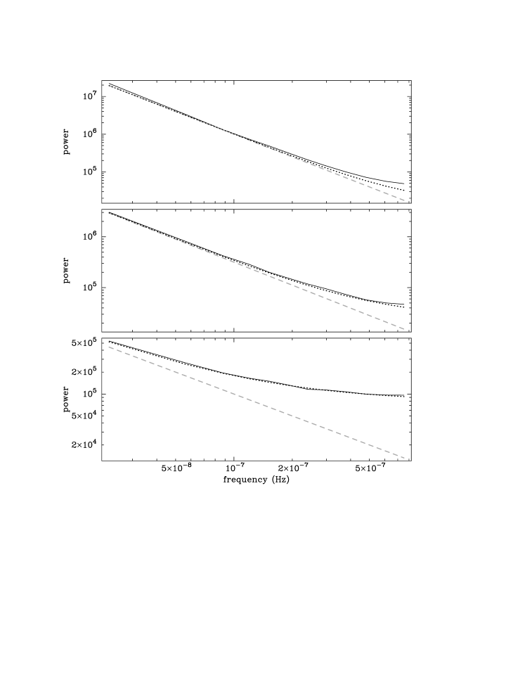
Figure 6: The effects of aliasing on power-spectral shape. The grey dashed line represents the true underlying power spectrum, while the solid black line shows the average observed power spectrum after distortion by the effects of discrete sampling at weekly intervals, obtained from averaging the power spectra of 1000 simulated lightcurves of 2-year duration (see text). The dotted line shows our approximation to the average observed power spectrum, obtained by assuming that the effect of aliasing is to add a constant to the underlying power spectrum. Underlying power spectral slopes from top to bottom are $\alpha=$2.0, 1.5 and 1.0 respectively.

Fortunately, the distorting effects of aliasing can be properly taken account of using the Monte Carlo technique mentioned earlier. The approximation to the distorting effect of aliasing presented here will prove useful for reducing the resolution of the simulated lightcurves required by the technique, as we will show in Section 4.1.

3.4 Stationarity of the power spectrum

A key assumption we must make, in order to combine lightcurves obtained at different times to measure the broadband power spectrum, is that the underlying power spectrum is stationary, i.e. its amplitude and shape do not change over time (note that power-spectral non-stationarity is not the same as lightcurve non-stationarity, which is expected on short time-scales for red-noise processes). If the underlying power spectrum were non-stationary, so that it happened to be steeper while the high-frequency power spectrum was measured than when the medium or low frequency power spectra were measured, then these changes in power-spectral slope would masquerade as a flattening in the power spectrum.
The power spectra of BHXRBs are known to be non-stationary on a variety of time-scales, showing drastic changes in shape between the well-known low and high states (e.g. Cui et al. 1997). Transitions between these states occur on time-scales of months to years and less drastic changes in power-spectral shape within the low and high states occur on time-scales of days or weeks (e.g. changes in the high-frequency slope and the position of the power-spectral breaks, Belloni & Hasinger 1990, Cui et al. 1997). If the variability time-scales for this kind of non-stationarity scale linearly with black hole mass, we would expect to see similar changes in the power spectra of AGN on time-scales of centuries or longer - much greater than the time-scale we can sample. This picture is supported by the fact that, to date, no hard evidence for non-stationarity in power-spectral shape has been reported for AGN. Hence it is probably safe to assume that the shapes of our target’s power spectra do not vary during the course of our monitoring campaign.
An alternative concern is that the amplitude of the power spectrum varies over time, even though the shape does not. In a separate paper, we report the intriguing (and unexpected) result that the X-ray RMS variability of Cyg X-1 and the accreting millisecond pulsar SAX J1808.4-3658 scale linearly with the local mean flux (Uttley & M^cHardy 2001). In other words, the fractional RMS (i.e. RMS divided by mean flux) measured for any fixed-length segment of the lightcurve is constant (subject to the stochastic variability inherent in the lightcurves), irrespective of the segment’s mean flux. We also confirm that the same property applies to the lightcurves of AGN and hence appears to be an important characteristic of the broadband noise variability in compact accreting systems. It is obvious then that we must always normalise our lightcurves by their mean before calculating their power spectra or, as we do here, divide their power spectra by the square of the mean, otherwise the shape of our broadband power spectrum will be dependent on the mean object flux at the time we measured each lightcurve.

4 psresp: a reliable method of estimating power-spectral shape

In order to take proper account of the errors on the power spectrum and the distorting effects due to rebinning, red-noise leak and aliasing, we must use a Monte Carlo technique to estimate the underlying power-spectral shape (and its uncertainty). The basic concept is to simulate a large number of continuous lightcurves with a known underlying power-spectral shape, apply the sampling pattern of the observed lightcurve, rebin and interpolate as necessary, obtain the resulting distorted power spectra and average them to determine the mean shape of the distorted model power spectrum. The spread of the simulated power spectra about the mean can be used to estimate the errors on the observed power spectrum. Applying the sampling pattern to a simulated (i.e. model) lightcurve before measuring its power spectrum is equivalent to convolving the window function of the sampling pattern with the Fourier transform of the model lightcurve to obtain the Fourier transform of the observed lightcurve. The effect is then similar to that used in X-ray spectral measurement, when a model spectrum is postulated and then convolved with the ‘response function’ of the detector to yield the ‘observed’ model spectrum which can be tested against the data. Hence, this Monte-Carlo technique for estimating the true power-spectral shape is known as the ‘response method’.
The response method was applied by Done et al. (1992), to measuring the power spectrum of unevenly sampled Ginga lightcurves and has subsequently been applied to ROSAT data (Green, M^cHardy & Done 1999). In both cases the method was applied only to a single lightcurve, of relatively short (a few days) duration. Here, however, we wish to fit the same power-spectral model to several power spectra in order to estimate the shape of the broadband power spectrum. We should not fit power spectra measured over different frequency ranges separately, because the distorting effects of aliasing and red-noise leak, which we must take account of, are dependent on the shape of the underlying power spectral shape outside the frequency range measured by a single power spectrum. Furthermore, the response method of Done et al. (1992) estimates a goodness of fit based on the standard $\chi^{2}$ statistic, which is not a reliable estimator for the distorted power spectra considered here and hence cannot be used to formally estimate fit probabilities. Therefore, for our purpose of reliably constraining the shape of the broadband power spectrum of AGN, we have developed a more sophisticated technique based on the response method, which we call psresp (for power spectral response). In the remainder of this section, we describe psresp in detail.

4.1 Lightcurve simulation

We simulate lightcurves using the method of Timmer & König (1995), which is superior to the commonly used method of summing sine waves with randomised phases in that the power-spectral amplitude at each frequency is randomly drawn from a $\chi^{2}$ distribution, as should be the case for noise processes, and not fixed at the amplitude of the underlying power spectrum. We create the fake ‘observed’ lightcurves as follows.
First, we specify a power-spectral model which we wish to test against the data (which is some continuous function such as a power-law, with or without breaks). The normalisation of the model power spectrum is a multiplicative factor which is carried through any convolution with the window function (i.e. only the power-spectral shape is distorted by sampling). Hence we can choose an arbitrary model normalisation and simply renormalise the resulting distorted model power spectrum to obtain the best possible fit to the data.
For each observed lightcurve used to measure the broadband power spectrum, we simulate $N$ continuous lightcurves using the given power-spectral model (where $N$ is large, between 100 and 1000). Ideally, the time resolution of the simulated lightcurves, $\Delta T_{\rm sim}$ should be the same as the initial resolution of the observed lightcurve $\Delta T_{\rm bin}$, which for our monitoring data is the typical exposure time of the snapshot observations. This is because any variations on time-scales down to this resolution will contribute to aliasing. Although we have derived an analytical approximation to the effect of aliasing on the power spectrum, this only tells us the average effect of aliasing for lightcurves which are evenly sampled. Due to the stochastic nature of the lightcurves, the actual power above the Nyquist frequency is variable and hence aliasing contributes a variable amount to the power spectrum which adds to the uncertainty in its shape. However, for the monitoring lightcurves, which consist of only 1 ksec snapshots but may be months or years long, the requirement that the simulated lightcurves also have 1 ksec resolution increases the computation time prohibitively.
In practice, we can limit the resolution of the simulated lightcurves to be $\Delta T_{\rm sim}\leq 0.1\Delta T_{\rm samp}$. This is because, for lightcurves whose power spectra are steep at high frequencies, like those we measure here, the uncertainty in the amount of aliasing is dominated by the uncertainty in the large amount of power at frequencies not much greater than the Nyquist frequency. We can then estimate the much smaller contribution to aliasing due to power at frequencies greater than sampled by the simulated lightcurves using our analytical approximation, i.e. calculating the integrated power of the model power spectrum between $(2\Delta T_{\rm sim})^{-1}$ and $(2\Delta T_{\rm bin})^{-1}$ (see Section 3.3) and incorporating the resulting constant values into the final simulated power spectra.
In order to take account of red-noise leak, the simulated lightcurves must be significantly longer (e.g. by a factor 10 or more) than the observed lightcurve, so that there is power at frequencies lower than the minimum frequency sampled by the observed lightcurve. We can minimise the cost of simulating excessively long lightcurves by making a single, very long lightcurve of length $NT$, which is subsequently split into the $N$ desired segments. Note that although the longest time-scale trends in the total simulated lightcurve contribute the same amount to the red-noise leak in the power spectra of all $N$ simulated lightcurve segments, the bulk of red-noise leak (and the power-spectral uncertainty it introduces) is due to variations on shorter time-scales close to the observed lightcurve duration and hence will be statistically independent between segments.
Once a continuous lightcurve is simulated, it is resampled using the same sampling pattern as the observed lightcurve. The resampled lightcurve is then rebinned and empty bins interpolated in the same manner as for the observed lightcurve. The power spectrum of the resulting lightcurve is then measured.

4.2 Determining the goodness of fit of the model

The power spectrum of each simulated lightcurve is calculated and binned in the same way as the power spectrum of the original observed lightcurve. The model average power spectrum (corresponding to the given model and sampling pattern of the observed lightcurve) is then given by the mean of the $N$ simulated power spectra, $\overline{P_{\rm sim}}(\nu)$. For each frequency $\nu$ sampled by the binned power spectrum, we determine the RMS spread of simulated model powers about the mean and define this spread to be the ‘RMS error’ on the power at that frequency, $\Delta\overline{P_{\rm sim}}(\nu)$. We next define a statistic, which we call $\chi^{2}_{\rm dist}$, which is calculated from the model average (and RMS error) and observed power spectra of each lightcurve:

$$\chi^{2}_{\rm dist}=\sum_{\nu=\nu_{\rm min}}^{\nu_{\rm max}}\frac{\left(\overline{P_{\rm sim}}(\nu)-P_{{\rm obs}}(\nu)\right)^{2}}{\Delta\overline{P_{\rm sim}}(\nu)^{2}},$$

where $\nu_{\rm min}$ and $\nu_{\rm max}$ are respectively the minimum and maximum frequencies measured by $P_{{\rm obs}}(\nu)$. We measure $\chi^{2}_{\rm dist}$ for each input power spectrum (i.e. low, medium and high-frequency), and sum to yield a total $\chi^{2}_{\rm dist}$ for the model with respect to the data. Note that although the approach of assigning error bars to the model rather than the data is unusual, it is technically valid and strictly speaking the more correct thing to do, since the $\chi^{2}$ statistic is defined on the basis of the variance of the model population, which error bars conventionally determined from the data are supposed to approximate (e.g. see discussion in Done et al. 1992, Section 4.2).
Next, we find the best-fitting normalisation of the power-spectral model by renormalising the $\overline{P_{\rm sim}}(\nu)$ for each input power spectrum by the same factor $k$, varying $k$ until the total $\chi^{2}_{\rm dist}$ is minimised.
Having determined the minimum $\chi^{2}_{\rm dist}$ for the model compared to the data, we next estimate what goodness of fit this value of $\chi^{2}_{\rm dist}$ corresponds to. The $\chi^{2}_{\rm dist}$ is not the same as the standard $\chi^{2}$ distribution, because the $P_{\rm obs}(\nu)$s are not normal variables (since the number of power spectrum estimates averaged in each frequency bin is small). Therefore we must estimate a reliable goodness of fit using the distribution of $\chi^{2}_{\rm dist}$ and not the well-known $\chi^{2}$ distribution. For each input low, medium and high-frequency power spectra, we have already created $N$ corresponding simulated power spectra which can be used to determine the distribution of $\chi^{2}_{\rm dist}$ for that particular model and lightcurve sampling pattern. In order to determine the distribution of $\chi^{2}_{\rm dist}$, we should calculate the values of $\chi^{2}_{\rm dist}$ for all possible combinations of simulated low, medium and high-frequency power spectra. However, since the number of such combinations ($N^{3}$) may be extremely large, we reduce the number of combinations we sample to $M$ (where $M\geq 1000$), randomly selected to ensure an accurate estimate of the distribution of $\chi^{2}_{\rm dist}$.
We sort the $M$ simulated measurements of the total $\chi^{2}_{\rm dist}$ into ascending order. The probability that the model can be rejected is then given by the percentile of the simulated $\chi^{2}_{\rm dist}$ distribution above which $\chi^{2}_{\rm dist}$ exceeds that measured for the observed power spectra. Note that this method of using simulated data sets to estimate goodness of fit in the absence of a well-understood fit statistic is well-known and described in Press et al. (1992), Section 15.6.

4.3 Incorporating VHF power spectra

As described in Section 3.1, we use continuous segments of the 16 s binned long-look lightcurves to make VHF power spectra for our most variable targets, by averaging the power spectra of all the segments and determining the standard error from the spread in power at each frequency. The standard errors estimated from the data are reliable, since we average $>20$ power spectra and bin the logarithm of power (according to the method of Papadakis & Lawrence 1993 and see Section 3.2). We can therefore use the measured VHF power spectra and their errors as they are, without having to estimate errors using simulations of high-resolution lightcurves which would be very computationally intensive. However, if we simply compare the VHF power spectrum with the underlying undistorted model shape, we ignore the effects of red-noise leak which could be significant in distorting the shape of the VHF power spectrum, especially if the underlying power spectrum does not flatten significantly until far below the minimum frequency sampled by the VHF power spectrum. Therefore, we need to take account of the effects of red-noise leak on the model power-spectral shape at high frequencies. Note that, because the segments are continuous and binned into high-resolution time bins of width 16 s, the effects of aliasing are not important in this case.
To determine the effects of red-noise leak on the VHF power spectrum, we simulate 1000 lightcurves, each made to be at least 64 times longer than $\nu_{\rm min}^{-1}$ (where $\nu_{\rm min}$ is the minimum frequency sampled by the VHF power spectrum), with resolution $\Delta T_{\rm sim}$ smaller than $\frac{1}{2}\nu_{\rm max}^{-1}$ where $\nu_{\rm max}$ is the maximum frequency which contains significant power above the noise level (typically around $3\times 10^{-3}$ Hz) and is chosen so that the ratio of $\nu_{\rm max}$ to $\nu_{\rm min}$ is a power of 2. Power spectra of the lightcurves sampled to have duration $\nu_{\rm min}^{-1}$ may then be made using the Fast Fourier Transform, which allows a VHF model average power spectrum for 1000 simulated lightcurves to be determined very rapidly. The VHF model average power spectrum is then used in place of the underlying model power spectrum, while the errors determined from the observed VHF power are used as errors on the model.
The contribution of the VHF power spectrum to the total $\chi^{2}_{\rm dist}$ is determined by comparing the observed power spectrum with the simulated model average power spectrum, using the standard errors estimated from the data. The contribution of the VHF power to the goodness of fit of the model is obtained as follows: for each of the $M$ random combinations of simulated power spectra used to estimate the goodness of fit, a VHF power spectrum is simulated by randomly selecting the power at each measured frequency, from a Gaussian distribution of mean equal to the model average power and standard deviation equal to the standard error at that frequency. The $\chi^{2}_{\rm dist}$ of the simulated VHF power spectrum is determined and included in the total $\chi^{2}_{\rm dist}$ measured for that selection of simulated power spectra. The goodness of fit of the model is then estimated as described in the preceding section.

4.4 Summary of the psresp method

We summarise the psresp method as follows:

1. Measure the observed power spectrum of each (rebinned and mean-subtracted) observed lightcurve and bin up the power spectrum as desired (see Section 3.1). Measure the VHF power spectrum if required, determining its errors directly from the data (see Section 4.3).

2. Specify the underlying power spectral model to be tested against the data. For the given set of parameters, simulate $N$ lightcurves which are realisations of the model and apply the sampling pattern of the observed lightcurve to the simulated lightcurves (see Section 4.1).

3. Calculate the power spectrum of each re-sampled simulated lightcurve using the same method used to measure the observed power spectrum. Determine the model average power spectrum from the $N$ simulated power spectra, and assign error bars equal to the RMS spread in simulated power at each frequency (see Section 4.2).
   The two steps above should be repeated for each lightcurve (i.e. long-term, intensive and long-look), to make simulated model average power spectra corresponding to each observed power spectrum. The model average VHF power spectrum should also be determined at this point (if required), according to the method outlined in Section 4.3.

4. Estimate the statistic $\chi^{2}_{\rm dist}$ (summed over all input power spectra) for the observed versus the model average power spectrum, and vary the normalisation of the model to minimise $\chi^{2}_{\rm dist}$ and obtain the best-fitting normalisation (include the VHF power spectrum in this determination if required, using standard errors determined from the data, see Section 4.3).

5. Determine the $\chi^{2}_{\rm dist}$ for $M$ randomly selected combinations of the simulated power spectra. If a VHF power spectrum is included, measure its contribution to each simulated total $\chi^{2}_{\rm dist}$ from a random realisation of the model average VHF power spectrum, according to the method described in Section 4.3. Sort the simulated distribution of $\chi^{2}_{\rm dist}$ into increasing numerical order - the model is rejected at a confidence equal to the percentile of the simulated $\chi^{2}_{\rm dist}$ distribution above which $\chi^{2}_{\rm dist}$ exceeds that measured for the observed power spectra (see Section 4.2).

Using the method described above, any given model can be tested against the data. By stepping through a range of model parameters and repeating steps 2–5, large regions of the model parameter space may be searched and confidence regions may be determined.

5 Results

We will now apply the psresp method described in Section 4 to the lightcurves of our sample, in order to determine if the broadband power spectra of Seyfert galaxies really flatten towards low frequencies and to try to constrain models for any flattening which we see.

5.1 Do the broadband power spectra really flatten?

To determine if the power spectra flatten, we will test a simple power-law model for the underlying power spectrum, $P_{\rm mod}(\nu)$ of the form:

$$P_{\rm mod}(\nu)=A\,\left(\frac{\nu}{\nu_{0}}\right)^{-\alpha}+C_{\rm noise},$$

where $A$ is the amplitude of the model power spectrum at a frequency $\nu_{0}$, $\alpha$ is the power-spectral slope and $C_{\rm noise}$ is a constant value which is fixed at the Poisson noise level for the lightcurve. Note that the Poisson noise level is included in the model rather than subtracted from the power spectra before model fitting, because the power spectra are binned logarithmically (so constants in linear space may not simply be subtracted). This is particularly important for the VHF power spectra of NGC 5506 and MCG-6-30-15, whose standard errors are determined in logarithmic space, and also for high-frequency power spectra in general, which are close to the Poisson noise level, since fluctuations in the power spectrum lead to some measured powers lying below the Poisson noise level (so subtraction of this level would lead to negative measured powers).
The model is tested against the measured power spectra by stepping through values of $\alpha$ from 1.0 to 2.4 in increments of 0.1 (i.e. test the model with $\alpha=1.0$, 1.1, 1.2 etc.). These values of $\alpha$ cover the range of reasonable values which could possibly be fitted to the data. Probabilities that the measured power spectra could be a realisation of the model are calculated by psresp, as described in Section 4.2 using $N=1000$ simulated lightcurves to determine the distorted model average power spectrum. The distribution of $\chi^{2}_{\rm dist}$ of the realisations of the model is determined for each value of $\alpha$ by measuring $\chi^{2}_{\rm dist}$ for $M=10^{4}$ randomly selected sets of simulated power spectra. The simulated lightcurves have time resolutions $\Delta T_{\rm sim}$ given in Table 3. Additional distortion in the power spectrum due to model power at frequencies greater than $(2\Delta T_{\rm sim})^{-1}$ is calculated directly from the model, as described in Section 4.1. Distorted VHF model power spectra, which take account of red-noise leak in the VHF power spectra included in the broadband power spectra of MCG-6-30-15 and NGC 5506, are determined using the method described in Section 4.3.

Table 3: Time resolution of simulated lightcurves used in psresp.

	Long-term	Intensive	Long-look
MCG-6-30-15	86400 s	8640 s	512 s
NGC 5506	86400 s	8640 s	512 s
NGC 5548	86400 s	8640 s	512 s
NGC 3516	46080 s	4608 s	512 s

The best-fitting values of $\alpha$, and corresponding confidences that the single power-law model is rejected by the data, are given in Table 4. The first and second of each of these values shown for NGC 5506 correspond to fits without or including the EXOSAT data respectively. The simple power-law model, without any flattening is rejected at better than 99% confidence for MCG-6-30-15, better than 90% confidence (or close to 99% confidence including the EXOSAT data) for NGC 5506 and better than 95% confidence for NGC 3516. Only for NGC 5548 is the model not rejected at a significant confidence. The best-fitting models are compared with the measured power spectra in Figure 7.

Figure 7: Comparison of best-fitting model average power spectra with the observed power spectra for the single power-law model described in the text. Open squares mark the low-frequency model average, simple crosses mark the high-frequency model average while filled squares mark the medium-frequency model average, the VHF model average for MCG-6-30-15 and NGC 5506, and the high-frequency model average for the second long-look observation of NGC 3516. Note that the error bars represent the RMS error in the simulated power spectra used to calculate $\chi_{\rm dist}^{2}$ as described in Section 4.2.

It is apparent from these plots that the simple power-law model does not fit the observed power spectra of MCG-6-30-15, NGC 5506 and NGC 3516, even after allowing for the distorting effects of sampling, because the intrinsic power spectrum of each of these objects does indeed flatten towards low frequencies. There is no significant evidence for flattening at low frequencies in the power spectrum of NGC 5548. Figure 8 shows the fit probability measured at each input value of $\alpha$ for NGC 5548, which demonstrates how psresp is capable of finding well-defined probability maxima in the same way that $\chi^{2}$ fitting can, using more conventional data sets.

Table 4: Results from fitting broadband power spectra of four Seyfert galaxies with a simple unbroken power-law model.

	Best-fitting $\alpha$	Rejection confidence
MCG-6-30-15	1.5	99.8%
NGC 5506	1.4/1.5	90.6%/98.6%
NGC 5548	1.6	67%
NGC 3516	1.8	96.6%

Quoted values for NGC 5506 correspond to fits excluding/including the EXOSAT data.

The simple power law model with no frequency breaks can be rejected at better than 95% confidence for all objects except NGC 5548. The next step is to try to fit the observed power spectra with more complex models which flatten at low frequencies, in particular, can we distinguish between models where the power spectrum flattens to $\alpha=0$ or $\alpha=1$, and can we constrain any characteristic frequencies for the flattening?

Figure 8: Probability that a single power-law of slope $\alpha$ is acceptable to describe the broadband power spectrum of NGC 5548.

5.2 Fitting simple models for the power-spectral flattening

Although we can say with confidence that the power spectra of three of the objects in our sample flatten towards low frequencies, it is not clear what form this flattening takes. In this work, we will restrict ourselves to considering two simple models, a ‘knee’ model based on the low-frequency flattening seen in the power spectra of BHXRBs in the low state (i.e. the low-frequency break in Cyg X-1) and a ‘high-frequency break’ model which assumes that the flattening is due to a frequency break in the power spectrum analogous to the high-frequency break seen in the power-spectrum of Cyg X-1. Under the knee model, the power-spectrum turns over to a slope $\alpha=0$ below some ‘knee frequency’, whereas under the high-frequency break model, the power spectrum breaks sharply to $\alpha=1$ below some ‘break frequency’. More complex models, consisting of multiple frequency-breaks and a variety of power-spectral slopes, or a number of broad Lorentzians (e.g. Nowak 2000) might also successfully explain the data. However, computational constraints limit the testing of a large variety of models for the flattening we see and moreover, as we shall discover, the data do not yet warrant these kinds of models as the observed power spectra can be fitted adequately by the simple models we test here. We will fit these two simple models for the flattening to the power spectra of all the Seyfert galaxies in our sample, including NGC 5548 so as to set upper limits on any knee or break frequencies.

5.2.1 The knee model

We first test the knee model for the power spectrum, which has the form

$$P(\nu)=\frac{A}{\left(1+\left(\frac{\nu}{\nu_{\rm knee}}\right)^{2}\right)^{\alpha/2}},$$

where $A$ is the constant amplitude of the power-spectrum at zero slope, $\nu_{\rm knee}$ is the ‘knee frequency’ and $\alpha$ is now defined as the power-spectral slope above the knee frequency. The shape which this function describes can be seen in Figure 9.

Figure 9: The form of the knee model power spectrum.

We now test this model against the measured broadband power spectra, to see if it can explain the flattening we see. Using the equation given above for the underlying power spectral shape (also including the constant Poisson noise level), we can fit the model in the same way as fitting a simple power law in the previous section. The free parameters to be stepped through are $\alpha$, which is again incremented in steps of 0.1 between 1.0 and 2.4, and $\nu_{\rm knee}$ which is stepped through by multiplicative factors of 2, from $10^{-8}$ Hz to $10^{-3}$ Hz, since a very broad range in frequency must be covered. Approximately 200 pairs of $\alpha$ and $\nu_{\rm knee}$ must be tested (as opposed to only 15 parameters when fitting the simple power law in the previous section), so to save on computing time, the number of lightcurve simulations used to estimate each model average power spectrum for each pair of parameters is reduced from $N=1000$ to $N=100$. The $\chi^{2}_{\rm dist}$ distribution is obtained by determining $\chi^{2}_{\rm dist}$ for $M=1000$ sets of simulated power spectra.
The best-fitting parameters and probabilities are shown in Table 5.

Table 5: Results from fitting broadband power spectra of four Seyfert galaxies with a knee model

	Rejection confidence	$\alpha$	$\nu_{\rm knee}/10^{-6}$ Hz
MCG-6-30-15	81%	$1.8\pm 0.1$	5.12 (2.56–10.24)
NGC 5506a	42%	$1.7\pm^{0.7}_{0.3}$	0.64 (0.0–10.24)
NGC 5506b	32%	$1.9\pm^{0.5}_{0.4}$	2.56 (0.16–10.24)
NGC 5548	53%	$1.6\pm^{0.8}_{0.2}$	0.02 (0.0–1.28)
NGC 3516	83%	$2.1\pm 0.3$	0.64 (0.32–1.28)

The table shows the confidence that the knee model can be rejected, the best fitting slope above the knee $\alpha$ and the best-fitting knee frequency $\nu_{\rm knee}$ and 90% lower and upper confidence limits to the knee frequency (in brackets). Errors quoted for $\alpha$ correspond to the values of $\alpha$ below which the fit probability is reduced to less than 10% (i.e. they represent 90% confidence limits). Note that these confidence limits are not interpolated between sampled points in the parameter space, unlike the confidence contours plotted in Fig. 10. The superscripts ^a and ^b mark the NGC 5506 results excluding and including the EXOSAT data respectively.

Figure 10: Comparison of best-fitting model average power spectra (points with error bars) with observed power spectra (lines) for the knee model described in the text (left), and corresponding confidence contours for the parameter space searched (right). The dashed and solid confidence contours represent the 68% and 90% confidence limits respectively.

Contour plots for each of the knee model fits (not including the fit of the NGC 5506 broadband power spectrum which excludes the EXOSAT data), together with the best-fitting model average power spectra, are shown in Figure 10. The contour plots show that the acceptable regions are broad and well-defined, rather than consisting of very many separate ‘islands’, which implies that using only 100 simulated lightcurves per measured power spectrum is sufficient to determine reliable maxima in the probability space.
As Table 5 shows, the knee model fits the power spectra of all the objects in our sample adequately. In all cases, the model can be accepted at a confidence level better than 10%. Note that the broadband power spectrum of NGC 5548 is consistent with this model, although the lower confidence limits on the knee frequency cannot be defined, in agreement with the acceptable simple power law fit to these data. The fact that the knee model provides a good fit to the broadband power spectrum of NGC 5506 including the EXOSAT data, is consistent with the power spectrum of NGC 5506 being stationary over time-scales as long as a decade.

5.2.2 The high-frequency break model

The motivation for the high-frequency break model comes from the power spectrum of the black hole X-ray binary Cyg X-1 in the low state, which shows two frequency breaks, as described in Section 1. If AGN have a similar power-spectral shape to Cyg X-1 (albeit scaled down in frequency by some factor), then because the power spectral slopes of AGN lightcurves measured at $>10^{-5}$ Hz by EXOSAT (e.g. Green, M^cHardy & Lehto 1993) are significantly greater than 1, we may be seeing the analog of the high-frequency break in Cyg X-1.
To test this possibility, we should try fitting the observed power spectra with a model of the form used to fit the high-frequency power spectrum of Cyg X-1 (e.g. Nowak 1999):

$$P(\nu)=\left\{\begin{array}[]{ll}A\,\left(\frac{\nu}{\nu_{\rm bk}}\right)^{-\alpha_{\rm hi}}&\mbox{if $\nu>\nu_{\rm bk}$}\\ A\,\left(\frac{\nu}{\nu_{\rm bk}}\right)^{-\alpha_{\rm lo}}&\mbox{otherwise}\end{array}\right.$$

Where $A$ is the power-spectral amplitude at the break frequency $\nu_{\rm bk}$, and $\alpha_{\rm hi}$ and $\alpha_{\rm lo}$ are the high and low-frequency slopes respectively, such that $\alpha_{\rm hi}>\alpha_{\rm lo}$. An example of a high-frequency break model with $\alpha_{\rm hi}=2$ and $\alpha_{\rm lo}=1$ is shown in Figure 11.

Figure 11: The form of the high-frequency break model power spectrum.

Note that there is no physical basis for the sharpness of the break in the high-frequency break model. However, since the model can adequately describe the high-frequency power-spectral shape of Cyg X-1, it should also serve as a possible empirical representation of the power spectra of poorer quality which we measure here. We do not consider the low-frequency break in this model in order to minimise the number of free parameters. This approach is valid since, if the model is correct, low-frequency breaks will occur at least a decade lower in frequency than any measured high-frequency breaks and so will not contribute as significantly to any flattening (besides which, if additional low-frequency breaks are significant they will be apparent from the residuals in any comparison of the data with the model).
We only consider a low frequency slope $\alpha_{\rm lo}=1$. Clearly it is desirable, on grounds of computation time, to restrict the number of free parameters by fixing the slope below the break, but there are also compelling observational reasons why we might fix the slope to $\alpha_{\rm lo}=1$. One particularly striking aspect of all the Cyg X-1 power spectra is that, despite the variations in the position of the high and low-frequency breaks and the slope above the high-frequency break (e.g. as shown by Belloni & Hasinger 1990), the slope of the intermediate power-spectrum, between the two breaks, is always remarkably close to 1. Furthermore, Nowak et al. (1999) show that the power spectra of Cyg X-1 made from simultaneous lightcurves in different energy bands show an energy dependence above the high-frequency break (in that $\alpha_{\rm hi}$ decreases towards higher energies) but maintain the same shape (i.e. $\alpha_{\rm lo}=1$) below the break. These results suggest that a power-spectral slope of 1 (or very close to 1) below the high-frequency break may, in fact, be the rule. We can determine if the power spectra we measure are at least consistent with this possibility by fitting the high-frequency break model (including the constant Poisson noise level, as before), fixing $\alpha_{\rm lo}=1$ and stepping through the same parameter ranges as used to fit the knee model (i.e. $\alpha_{\rm hi}=1.0$–2.4 in increments of 0.1, $\nu_{\rm bk}=10^{-8}$–10^-3 Hz in multiples of 2).
The resulting best-fitting parameters are shown in Table 6, with the results presented in the same format as for the knee model.

Table 6: Results from fitting the broadband power spectra of four Seyfert galaxies with a high-frequency break model

	Rejection confidence	$\alpha$	$\nu_{\rm bk}/10^{-6}$ Hz
MCG-6-30-15	33%	$2.0\pm 0.3$	51.2 (12.8–102.4)
NGC 5506a	10%	$2.1\pm^{0.3}_{0.7}$	25.6 (0.0–102.4)
NGC 5506b	3%	$2.4\pm^{0}_{0.9}$	51.2 (0.4–102.4)
NGC 5548	27%	$2.4\pm^{0}_{1.0}$	2.56 (0.0–10.24)
NGC 3516	39%	$2.2\pm^{0.2}_{0.3}$	2.56 (0.64–5.12)

See Table 5 for description.

The best-fitting model average power spectra and confidence contour plots are shown in Figure 12. The high-frequency break model is an acceptable description of the data at better than 10% confidence for all objects in the sample. The lower limit to break frequency is not constrained in the power spectrum of NGC 5548.

Figure 12: Comparison of best-fitting model average power spectra (points with error bars) with observed power spectra (lines) for the high-frequency break model described in the text (left), and corresponding confidence contours for the parameter space searched (right). The dashed and solid confidence contours represent the 68% and 90% confidence limits respectively.

6 Discussion

6.1 Summary of results

We find that the power spectra of three of the four Seyfert galaxies in our sample (MCG-6-30-15, NGC 5506, NGC 3516) flatten significantly at low frequencies and that the power-spectral flattening can be well-fitted by either a knee or a high-frequency break model. Although there is no significant evidence for low-frequency flattening in the power spectrum of NGC 5548, our model fits show that we cannot rule out the possibility of a knee or break in the power spectrum of this object also (at $\nu<10^{-6}$ Hz or $\nu<10^{-5}$ Hz for knee or break models respectively).
We stress that the detection of low-frequency flattening in the power spectra of AGN which we report here is completely robust, since it is based on a rigorous Monte Carlo technique which we use to formally reject the simple power-law model for the power spectrum. On the other hand, our measurements of characteristic knee or break frequencies for the flattening are model dependent, as can be seen by the fact that two different models for the flattening can fit the data. Clearly, the data are not yet adequate to distinguish between different models for the flattening.

6.2 Comparison with naive fits to the observed power spectrum

Our results confirm earlier indications of flattening in the power spectrum of NGC 5506 (M^cHardy 1989) and the evidence of flattening in the power-spectra of NGC 3516 and MCG-6-30-15 presented by Edelson & Nandra (1999) and Nowak & Chiang (2000) respectively. Chiang et al. (2000) also claim low-frequency flattening in the power spectrum of the RXTE ASM lightcurve of NGC 5548 but, as shown in Figure 2, ASM lightcurves of faint sources do not show the true source variability. All these claims of power-spectral flattening use a more ‘naive’ fit to the observed power spectrum, simply fitting the assumed model directly using the data to determine errors at each frequency, and taking no account of the distorting effects of aliasing or red-noise leak. The fact that we confirm the power-spectral flattening reported in these previous works raises the question: is it really necessary to use a Monte Carlo technique to fit the observed power spectra?
To answer this question, we naively fit the observed power spectra with the high-frequency break model, which the psresp method shows is a good fit to all the data. We bin the measured ‘raw’ power spectra (obtained from the rebinned and interpolated lightcurves, see Section 3.1) in logarithmically spaced bins, separated by a factor of 2 in frequency (e.g. Edelson & Nandra 1999), using a minimum of four measured frequencies per bin. We determine the standard error from the spread in measured powers in each bin. The binned power spectra and best-fitting high-frequency break models are shown in Figure 13 and comparison of the best-fitting parameters with those obtained using Monte Carlo fits are shown in Table 7.

Figure 13: Best-fitting high-frequency break models (solid lines) fitted naively to binned observed power spectra (points with error bars). Error bars are standard errors determined from the data. To illustrate aliasing effects we also show the best-fitting underlying power spectral models obtained from the Monte Carlo fits (dashed lines), using the broken power law model for all sources excpet NGC 5548, where we show the simple power law (see text for discussion).

Table 7: Comparison of naively fitted break model parameters with Monte Carlo results

	Naive results			Monte Carlo results
	$\chi^{2}$/d.o.f.	$\alpha$	$\nu_{\rm bk}/10^{-6}$ Hz	$\alpha$	$\nu_{\rm bk}/10^{-6}$ Hz
MCG-6-30-15	59.6/22	1.68	5.43	$2.0\pm 0.3$	51.2 (12.8–102.4)
NGC 5506	25.2/20	$1.95\pm^{0.22}_{0.16}$	20.0 (9.2–44.2)	$2.4\pm^{0}_{0.9}$	51.2 (0.4–102.4)
NGC 5548	17.2/11	$1.9\pm^{0.18}_{0.2}$	0.87 (0.18–1.9)	$2.4\pm^{0}_{1.0}$	2.56 (0.0–10.24)
NGC 3516	60.16/22	2.06	1.9	$2.2\pm^{0.2}_{0.3}$	2.56 (0.64–5.12)

The table shows the $\chi^{2}$ (and degrees of freedom), slope above the break, $\alpha$ and break frequency, $\nu_{\rm bk}$ obtained from naive model fits, and for comparison the model parameters estimated from the Monte Carlo fits using psresp (see Section 5.2.2). Errors are 90% confidence, corresponding to $\Delta\chi^{2}=4.61$ in the naive fits. Errors are not quoted where the fit is very bad.

The first point to note is that most of the error bars on the observed power spectra are much smaller than we would expect given the spread in power indicated by simulated power spectra. This is because the power at each Fourier frequency is randomly distributed with an exponential ($\chi^{2}_{2}$) distribution, hence if only a few points are sampled the spread in points is likely to be small. A larger number of points ($>20$) must be averaged in each bin in order that error bars determined from the data are reliable (see Section 3.2). Because the errors are underestimated, the best quality broadband power spectra (for MCG-6-30-15 and NGC 3516, which have more extensive long-look and intensive monitoring lightcurves respectively) are badly fitted by the model. Better fits are obtained for the poorer quality data (for NGC 5506 and NGC 5548), but the 90% confidence errors on the model parameters are greatly underestimated, so that naive fitting implies that the flattening in the power spectrum of NGC 5548 is significant, whereas Monte Carlo fits show that it is not.
The underestimation of errors is a major problem for naive model fitting, which must be taken into account when considering claims of power-spectral flattening in the literature. For example, Nowak & Chiang (2000) claim a second, significant low-frequency break at $\sim 10^{-5}$ Hz (flattening to zero slope) in the power spectrum of MCG-6-30-15, measured from long-look data alone. Our simulations show that this additional flattening is not significant. Furthermore, our simulations show that the best-fitting model of Nowak & Chiang, when applied to the entire broadband power spectrum, is ruled out at $>99$% confidence: there is significant power at lower frequencies than $10^{-5}$ Hz.
We now note the effects of aliasing on naive model fits to observed power spectra. To illustrate aliasing effects, we show the best-fitting high-frequency break models from the Monte Carlo fits (i.e. unmodified by aliasing or the Poisson noise level) in Figure 13 as dotted lines (except for NGC 5548, where we show the unbroken power law model, which was an acceptable fit to the data). Monte Carlo fits show that the power spectrum of NGC 3516 is steep at high frequencies ($\alpha\sim 2$). Therefore, since there is little high-frequency power, the amount of aliasing at lower frequencies is small and thus the naive fitting of a break model produces similar results to those obtained by Monte Carlo fits. Similarly, the naive fits to the power spectrum of NGC 3516 carried out by Edelson & Nandra (1999) yield a similar knee frequency to that measured using simulations ($\nu_{\rm knee}\sim 4\times 10^{-7}$ Hz versus $\sim 6\times 10^{-7}$ Hz respectively).
In contrast to the case of NGC 3516, the X-ray lightcurve of MCG-6-30-15 contains significant power up to high frequencies, and hence the effects of aliasing are much more significant, especially in the low frequency power spectrum, determined from the long-term lightcurve which has the largest sampling interval. The result of this aliasing is a discontinuity in the measured broadband power spectrum from the medium to low-frequency parts of the power spectrum (reflected in the simulated model average power spectra, see Figure 10 and Figure 12), so that the low-frequency power spectrum appears flatter and may be signficantly raised above the medium-frequency power spectrum. This effect is apparent when we compare the best-fitting model obtained from the naive fits with that obtained by Monte Carlo fits (solid and dotted lines respectively in Figure 13): the high frequency end of the low-frequency power spectrum is raised significantly above the true power level by the effects of aliasing, so that in the naive fits, the position of the break is pushed to significantly lower frequencies than those estimated by the Monte Carlo fits. The same effect might also cause the apparent break, where none is actually required, in the power spectrum of NGC 5548, since the power spectrum in this case may be unbroken and have a relatively flat slope $\alpha=1.6$, which causes significant distortion due to aliasing in the high-frequency ends of both the medium and low-frequency power spectra.
Note that the distorting effect of aliasing is made worse by the fact that the high-frequency ends of the power spectra are also the most well-defined, as they are made by averaging over a large number of frequencies, so that systematic errors due to aliasing are more pronounced than they would be if the low-frequency ends of the power spectra were well sampled (since for red-noise power spectra, the aliased power at frequencies much lower than the Nyquist frequency is small compared to the underlying power). Because of this effect, particular caution should be applied to claims of low-frequency flattening based on naive fits to the power spectra of AGN which are highly variable on short time-scales (e.g. Akn 564, Pounds et al. 2001).
Under what circumstances might naive fitting produce reliable results (and associated uncertainties)? Clearly, the effects of aliasing can be mitigated by binning up the lightcurves to a longer sampling interval, thus smoothing out the variability on time-scales less than the sampling interval used to make the power spectrum. Unfortunately, the effect of this binning is to reduce the Nyquist frequency and hence the frequency range sampled by the power spectra. Furthermore, since reliable errors may only be estimated by averaging over $<20$ points per frequency bin, the lowest frequency sampled in our observed power spectra would have to be increased by a factor $\sim 10$, in order that sufficient low-frequency power-spectral points are averaged over. The net effect of binning up the lightcurves and power spectra is to reduce the frequency range covered by the individual low and medium-frequency power spectra by $\sim 2$ decades (i.e. to virtually a single frequency bin in each), while the low-frequency end of the high-frequency power spectrum (which does not suffer so much from aliasing) is shifted up by a decade.
Therefore, we conclude this discussion by noting that the naive method may be used to fit power spectra over relatively narrow ranges which are well sampled (i.e. the highest frequencies in AGN long-look lightcurves), but the Monte Carlo method of power-spectral fitting, of which psresp is an example, is essential in order to place reliable constraints on the underlying broadband power-spectral shape of AGN lightcurves obtained to date.

6.3 Estimating black hole masses

Having measured characteristic knee or break frequencies under the assumption of different underlying power-spectral models, we can consider the implications of the measured characteristic frequencies for the black hole mass. Throughout our discussion, we make the specific assumption that all the objects in our sample have the same power-spectral form (knee or break) so that the characteristic frequencies are directly comparable.
What is most striking about the characteristic frequencies measured for MCG-6-30-15 and NGC 3516 is that they are significantly different, in either model, at a level of better than 99% confidence, i.e. the 90% confidence limits of the break frequencies do not overlap. This is unexpected, because both objects have similar 2–10 keV X-ray luminosities of $L_{\rm 2-10}\sim 1.5\times 10^{43}$ erg s^-1, so the fundamental parameter driving the position of the characteristic frequency is not strictly related to the luminosity. One intriguing possibility is that although both objects have a similar luminosity, they may have different black hole masses. It is quite possible that the break or knee time-scales scale linearly with black hole mass, as would be expected if they correspond to a characteristic time-scale in the accretion disk or the characteristic size scale of the system. If this is the case, then MCG-6-30-15 must have a significantly smaller black hole than NGC 3516 and so must be accreting at a much higher fraction of its Eddington limit.
Let us assume that the characteristic frequency scales linearly with the inverse of black hole mass, and that the mass of the black hole in Cyg X-1 is 10 M_⊙ (Nowak et al. 1999). We will scale the best-fitting frequency measured by the knee model with the mean frequency of the low-frequency break in the low-state power spectrum of Cyg X-1, which varies between 0.04–0.4 Hz but has an average value of 0.13 Hz (taken from the 28 separate measurements presented in Belloni & Hasinger 1990). Similarly, we scale the best-fitting frequency measured in the high-frequency break model with the high-frequency break in the low-state power spectrum of Cyg X-1, with mean value 3.3 Hz, varying between 1–6 Hz. The resulting best estimates of black hole mass are shown in Table 8, together with conservative upper limits to the black hole mass, obtained by scaling the 90% confidence lower limits to knee/break frequency with the respective upper values of the observed knee/break frequency ranges in Cyg X-1 (i.e. 0.4 Hz and 6 Hz for knee and break frequencies respectively). We also show the corresponding bolometric luminosities expressed as a fraction of the Eddington luminosity for a black hole with the estimated mass, $L_{\rm Edd}\simeq 1.3\times 10^{38}\,M_{\rm BH}$ erg s^-1. For MCG-6-30-15, we assume the bolometric luminosity of $8\times 10^{43}$ erg s^-1, estimated from a multiwavelength study by Reynolds et al. (1997). For the remaining AGN, bolometric luminosities are derived from the typical 2–10 keV X-ray luminosities ($1.5\times 10^{43}$ ergs s^-1 for NGC 5506 and NGC 3516, $5\times 10^{43}$ ergs s^-1 for NGC 5548) by applying the mean bolometric correction of Padovani & Rafanelli (1988), $L_{\rm bol}\simeq 27L_{\rm 2-10}$. Note that scatter in this bolometric correction for individual sources, estimated from the measurements of Padovani & Rafanelli (1988) is possibly up to a factor $\sim 3$ in either direction. The bolometric correction for MCG-6-30-15 is a factor 5 lower than the mean value, but Reynolds et al. (1997) note that their estimate is a lower limit, based on the assumption of minimal reddening in this source, so that the bolometric luminosity in MCG-6-30-15 may be substantially larger than shown here.

Table 8: Black hole mass and bolometric luminosity estimates

	knee model				high-frequency break model
	best estimate		upper mass limit		best estimate		upper mass limit
	$M/10^{6}{\rm M_{\odot}}$	$L_{\rm bol}/L_{\rm Edd}$	$M/10^{6}{\rm M_{\odot}}$	$L_{bol}/L_{\rm Edd}$	$M/10^{6}{\rm M_{\odot}}$	$L_{\rm bol}/L_{\rm Edd}$	$M/10^{6}{\rm M_{\odot}}$	$L_{\rm bol}/L_{\rm Edd}$
MCG-6-30-15	0.25	2.4	1.6	0.4	0.6	1	5	0.14
NGC 5506	0.5	6	25	0.1	0.6	5	150	0.02
NGC 5548	65	0.2	NA	NA	13	0.8	NA	NA
NGC 3516	2	1.5	13	0.25	13	0.25	94	0.03

See text for details. Mass estimates for NGC 5506 use the model fit results for the RXTE plus EXOSAT data. No upper limits can be set on the black hole mass of NGC 5548.

Table 8 shows that, for the objects with the best-constrained characteristic frequencies in their power spectra (MCG-6-30-15 and NGC 3516), the knee model predicts a lower black hole mass than the high-frequency break model. Reverberation mapping estimates of the mass of NGC 3516 suggest a black hole mass of $\sim 2\times 10^{7}$ M_⊙ (Wanders & Horne 1994), compatible with the best estimate of mass from the high-frequency break model, but not inconsistent with the upper limit derived from the knee model. Given the uncertainty in the true bolometric luminosity, and the conservative upper mass limits quoted here, the masses predicted by the knee model are consistent with sub-Eddington accretion rates.
However, the conservative 40% Eddington lower limit to accretion rate estimated from the knee model fits to the power spectrum of MCG-6-30-15 (where the bolometric luminosity quoted represents a firm lower bound) is in contrast to that observed in Cyg X-1 where the transition between the low and high states occurs at only a few per cent of the Eddington luminosity (Di Salvo et al. 2001, Zhang et al. 1997). Since the knee model represents the low-frequency break seen in the power spectrum of Cyg X-1 in the low state, it would seem that the evidence from accretion rate is inconsistent with the knee model, at least in this source. Interestingly, even the high-frequency break model predicts an upper limit to black hole mass which is only barely consistent with the low-state accretion rates seen in Cyg X-1. An intriguing possibility is that MCG-6-30-15 is in a state analogous to the high state of Cyg X-1, which has a characteristic steep ($\alpha\simeq 2$) high-frequency power spectrum breaking at 10 Hz to $\alpha\simeq 1$, with no low-frequency breaks down to frequencies as low as $10^{-2}$ Hz (Cui et al. 1997). Therefore, high state power spectra similar in shape to that of Cyg X-1 would also be compatible with the high-frequency break model we use here. Scaling by the high state frequency-break yields an estimated black hole mass of $2\times 10^{6}$ M_⊙ (upper limit $\sim 8\times 10^{6}$ M_⊙), implying an accretion rate of $\sim 30$% Eddington (which we might expect from a high-state source).
Although the black hole mass in MCG-6-30-15 has not yet been measured by reverberation mapping, Reynolds (2000) has pointed out that the low luminosity (absolute B magnitude $\simeq-19$) of the S0 host galaxy of this AGN corresponds to a black hole mass of $\sim 10^{7}$ M_⊙ if the black hole mass-bulge luminosity relation is the same as that determined by Magorrian et al. (1998) for a sample of normal elliptical and S0 galaxies. We note here that the black hole masses of all the Seyfert galaxies which have been reverberation mapped show smaller black hole masses by a factor of $\sim 10$ than the Magorrian relation suggests (Wandel 1999). This discrepancy would imply a black hole mass for MCG-6-30-15 which is significantly lower than $10^{7}$ M_⊙, consistent with the low mass suggested by the high state interpretation of the power spectrum. We further note that the lower, reverberation mapping estimates of black hole mass in AGN also follow the recently discovered correlation of black hole mass with bulge velocity dispersion, which has been found to be a better predictor of black hole mass than the Magorrian relation (Gebhardt et al. 2000, Ferrarese et al. 2001). Therefore it seems plausible that the black hole in MCG-6-30-15 has a mass of order $10^{6}$ M_⊙. Reverberation mapping, or another independent mass estimation technique will be required to confirm this.
The power-spectral shape of NGC 5506 is also consistent with a high state interpretation of this source, although the uncertainties on the break frequency are sufficiently large that a low-state interpretation would suffice to fit the data self-consistently. We note here however that the low luminosity of the NGC 5506 galaxy (absolute B magnitude $\simeq-20$), suggests that the central black hole mass is relatively low. Although reverberation mapping of NGC 5506 is not possible because it is a Seyfert 2, it does have a water megamaser (Braatz, Wilson & Henkel 1994) which might permit a good estimate of its central black hole mass for comparison with the mass estimated from its power spectrum.
The high state AGN interpretation for either MCG-6-30-15 or NGC 5506 is highly speculative at this stage. One significant problem is that the energy spectra of neither source shows the steep power-law ($\Gamma\sim 2.6$) and strong disk blackbody components seen in the spectrum of Cyg X-1 in the high state (Cui et al. 1998), although this difference might be a result of the significantly lower disk temperature expected in AGN compared to BHXRBs. Greater support for the high state interpretation in either MCG-6-30-15 and NGC 5506 could be provided by the detection of significant power down to very low frequencies, implying that there is no low-frequency break in the power spectrum on frequencies $<0.01\nu_{\rm bk}$. Continued long-term monitoring will help to resolve this issue.
The frequency break in NGC 5548 is not signficantly detected. The black hole mass of NGC 5548 measured from reverberation mapping is $\sim 10^{8}$  M_⊙ (Wandel, Peterson & Malkan 1999), implying that the accretion rate is relatively low ($<10\%$ Eddington), so applying the low state interpretation we can estimate that the high-frequency break occurs at $\sim 2\times 10^{-7}$ Hz, and may become detectable with further monitoring observations.

6.4 The AGN-BHXRB connection and physical implications

The main result of this work has been to show that the power spectra of AGN flatten towards low frequencies. Whether this flattening has the same form as that in BHXRBs is still not certain. The data do not yet allow us to categorically rule out either knee or high-frequency break models, let alone more complex models where the power spectra might have multiple breaks or flatten gradually. However, it is encouraging that a simple high-frequency break, similar to that seen in the classic BHXRB Cyg X-1, can fit the data well, and yield plausible black hole masses if we assume that the break frequency scales inversely with black hole mass.

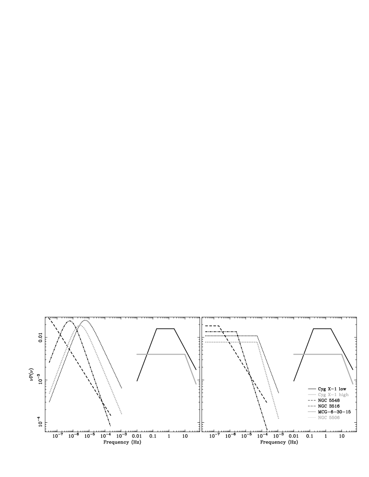
Figure 14: Comparison of best-fitting knee (left panel) and high-frequency break (right panel) model $\nu P(\nu)$ power spectra of MCG-6-30-15, NGC 5506, NGC 3516, NGC 5548 with power spectra of Cyg X-1 in the low and high states.

A useful way of comparing power spectra is to plot frequency$\times$power, rather than power, as a function of frequency. The $\nu P(\nu)$ plot produced in this way is analogous to the $\nu F(\nu)$ method of displaying energy spectra, in that the peak in the $\nu P(\nu)$ plot shows which time-scales most of the variability occurs on, as well as the magnitude of variability on those time-scales. In Figure 14 we plot the $\nu P(\nu)$ power spectra for the best-fitting knee and high-frequency break models fitted to the observed power spectra of MCG-6-30-15, NGC 5506 and NGC 3516 (see Section 5.2.2). The $\nu P(\nu)$ power spectra of NGC 5548 are also included in the figure, except that since the knee or break is not defined for this object, we have assumed knee and break frequencies of $10^{-8}$ Hz and $2\times 10^{-7}$ Hz respectively, corresponding to the black hole mass of $10^{8}$ M_⊙ estimated from reverberation mapping. For comparison, $\nu P(\nu)$ power spectra of Cyg X-1 are included, corresponding to typical power-spectral parameters in the low and high states (Nowak et al. 1999, Cui et al. 1997).
Note that the flat peaks in the high-frequency break $\nu P(\nu)$ power spectra of AGN and the typical power spectra of Cyg X-1 correspond to the $\alpha=1$ part of the power spectrum, where there is equal integrated power per decade of frequency. The low-frequency drop-off in the $\nu P(\nu)$ power in the low state of Cyg X-1 corresponds to the low-frequency break or ‘knee’ in the power spectrum, which we have not yet detected in the AGN power spectra if we are seeing the high-frequency break, because our low-frequency data is not yet adequate to detect it. Therefore, until clear evidence for low-frequency flattening to a slope $\alpha=1$ is found, we cannot rule out the possibility that all our sources have power spectra similar to the high state power spectrum in Cyg X-1.
Note that the knee model $\nu P(\nu)$ power spectra do not show flat peaks, because the high-frequency slopes fitted are all significantly steeper than 1. If we were measuring the low-frequency break alone (i.e. the frequency of the high-frequency break is too high to detect), we would expect the knee model to fit high-frequency slopes of $\alpha\simeq 1$. This result provides additional evidence that we are indeed measuring the high-frequency breaks in these sources, if the power spectra of AGN have the same shape as those of BHXRBs. However, we stress that we cannot yet rule out the possibility that we are measuring more complex configurations including both high and low-frequency breaks.
Fig. 14 shows clearly that the $\nu P(\nu)$ power spectra of AGN are similar to those in Cyg X-1, in that they have similar peak powers, but are shifted at least 5 decades down the frequency axis. The fact that the peak powers are similar implies that the number of varying regions and the general pattern of variability is the same in AGN and BHXRBs, while the luminosity of the varying regions and their variability time-scales are scaled by some factor which could be the black hole mass.

7 Conclusions

We have presented long-term RXTE monitoring lightcurves for 4 Seyfert galaxies, MCG-6-30-15, NGC 5506, NGC 5548 and NGC 3516, and measured their broadband power spectra to determine if they flatten towards low frequencies, like those of BHXRBs. The interpretation of power spectra measured from discretely (and sometimes unevenly) sampled lightcurves is complicated by the distorting effects of red-noise leak and aliasing. A further serious problem is that reliable errors in the power in each frequency bin cannot be defined from the data, due to the small number ($<20$) of power-spectral measurements in each frequency bin.
To overcome these difficulties, we have built on the response method of Done et al. (1992), to develop a reliable Monte Carlo method for testing models for the underlying power-spectral shape of discretely, unevenly sampled lightcurves. Our method, psresp, takes proper account of the effects of aliasing and red-noise leak and crucially, uses the distribution of simulated power spectra to define reliable confidence limits on our model fits.
We have used psresp to test simple models for the power-spectral shape of the active galaxies in our sample. Our main results are:

1. A single power-law model for the power spectra, with no low-frequency flattening, is rejected at better than 95% confidence for MCG-6-30-15, NGC 5506 and NGC 3516. The power spectrum of NGC 5548 is consistent with a single power-law.

2. Both the knee model (flattening to slope $\alpha=0$) and high-frequency break model (flattening to $\alpha=1$) provide good fits to the power spectra of all four sources. Knee/break frequencies are well constrained for all sources except NGC 5548, for which we can define upper limits only.

3. The characteristic knee/break frequency measured for MCG-6-30-15 is significantly higher (99% confidence) than the corresponding frequency in NGC 3516, even though both sources have similar X-ray luminosities ($\sim 1.5\times 10^{43}$ erg s^-1).

4. If the knees or breaks correspond to those seen in the low-state power spectrum of Cyg X-1, and the characteristic knee/break time-scales scale linearly with black hole mass, the black hole masses estimated from the knee model are lower than those estimated by the break model, but remain consistent with sub-Eddington accretion rates. In the case of MCG-6-30-15, the conservative lower limit on accretion rate estimated from the knee model is an order of magnitude higher than that seen in the low state of Cyg X-1, favouring the high-frequency break model and further suggesting that the break seen in the power spectrum of MCG-6-30-15 (and possibly NGC 5506) is analogous to the high-frequency break seen in the high state power spectrum of Cyg X-1.

5. The $\nu P(\nu)$ power spectra of the Seyfert galaxies studied here are similar in amplitude to the $\nu P(\nu)$ power spectra of Cyg X-1 in the high and low states.

Conclusions 4 & 5 imply that the power spectra of AGN are consistent with being identical in shape and fractional RMS amplitude (integrated over the whole power spectrum) to those of BHXRBs, with characteristic time-scales scaling linearly with black hole mass. Arguments based on accretion rate seem to favour the high-frequency break model over the knee model in at least one source (MCG-6-30-15), although this evidence is circumstantial. Further monitoring observations (which are currently underway) are needed to reject either model on the basis of power-spectral measurements alone, and to confirm the interesting possibility that two of the objects in our sample are analogous to high-state BHXRBs.

Acknowledgments

We would like to thank the entire RXTE team for making this work possible, and the anonymous referee, for helpful comments and suggestions. This research has made use of data obtained from the High Energy Astrophysics Science Archive Research Center (HEASARC), provided by NASA’s Goddard Space Flight Center.

References

- [Belloni & Hasinger 1990] Belloni T., Hasinger G., 1990, A&A, 227, L33
- [Braatz, Wilson & Henkel 1994] Braatz J. A., Wilson A. S., Henkel C., 1994, ApJ, 437, L99
- [Chiang et al. 2000] Chiang J., Reynolds C. S., Blaes O. M., Nowak M. A., Murray N., Madejski G., Marshall H. L., Magdziarz P., 2000, ApJ, 528, 292
- [Cui et al. 1997] Cui W., Zhang S. N., Focke W., Swank J. H., 1997, ApJ, 484, 383
- [Cui et al. 1998] Cui W., Ebisawa K., Dotani T., Kubota A., 1998, ApJ, 493, L75
- [Deeming 1975] Deeming T. J., 1975, Astrophys. & Space Sci., 36, 137
- [Di Salvo et al. 2001] Di Salvo T., Done C., Zycki P. T., Burderi L., Robba N. R., 2001, ApJ, 547, 1024
- [Done et al. 1992] Done C., Madejski G. M., Mushotzky R. F., Turner T. J., Koyama K., Kunieda H., 1992, ApJ, 400, 138
- [Edelson & Nandra 1999] Edelson R., Nandra K., 1999, ApJ, 514, 682
- [Ferrarese et al. 2001] Ferrarese L., Pogge R. W., Peterson B. M., Merritt D., Wandel A., Joseph C. L., 2001, ApJ, 555, L79
- [Gebhardt et al. 2000] Gebhardt K. et al., 2000, ApJ, 543, L5
- [Green, McHardy & Lehto 1993] Green A. R., McHardy I. M., Lehto H. J., 1993, MNRAS, 265, 664
- [Green, McHardy & Done 1999] Green A. R., McHardy I. M., Done C., 1999, MNRAS, 305, 309
- [Lamer et al. 2000] Lamer G., Uttley P., McHardy I. M., 2000, MNRAS, 319, 949
- [Lawrence et al. 1987] Lawrence A., Watson M. G., Pounds K. A., Elvis M., 1987, Nat, 325, 694
- [Lawrence & Papadakis 1993] Lawrence A., Papadakis I., 1993, ApJ, 414, L85
- [Lee et al. 1999] Lee J. C., Fabian A. C., Brandt W. N., Reynolds C. S., Iwasawa K., 1999, MNRAS, 310, 973
- [Magorrian et al. 1998] Magorrian J. et al., 1998, AJ, 115, 2285
- [McHardy 1988] McHardy I. M., 1988, MmSAI, 59, 239
- [McHardy & Czerny 1987] McHardy I. M., Czerny B., 1987, Nat, 325, 696
- [Nandra et al. 1997] Nandra K., George I. M., Mushotzky R. F., Turner T. J., Yaqoob T., 1997, ApJ, 476, 70
- [Nowak 2000] Nowak M. A., 2000, MNRAS, 318, 361
- [Nowak & Chiang 2000] Nowak M. A., Chiang J., 2000, ApJ, 531, L13
- [Nowak et al. 1999] Nowak M. A., Vaughan B. A., Wilms J., Dove J. B., Begelman M. C., 1999, ApJ, 510, 874
- [Padovani & Rafanelli 1988] Padovani P., Rafanelli P., 1988, A&A, 205, 53
- [Papadakis & Lawrence 1993] Papadakis I. E., Lawrence A., 1993, MNRAS, 261, 612
- [Papadakis & McHardy 1995] Papadakis I. E., McHardy I. M., 1995, MNRAS, 273, 923
- [Pounds et al. 2001] Pounds K., Edelson R., Markowitz A., Vaughan S., 2001, ApJ, 550, L15
- [Press et al. 1992] Press W. H., Teukolsky S. A., Vetterling W. T., Flannery B. P., 1992, Numerical Recipes, Second edition
- [Reynolds 2000] Reynolds C. S., 2000, ApJ, 533, 811
- [Reynolds et al. 1997] Reynolds C. S., Ward M. J., Fabian A. C., Celotti A., 1997, MNRAS, 291, 403
- [Timmer & König 1995] Timmer J., König M., 1995, A&A, 300, 707
- [Uttley & McHardy 2001] Uttley P., McHardy I. M., 2001, MNRAS, 323, L26
- [Uttley et al. 1999] Uttley P., McHardy I. M., Papadakis I. E., Guainazzi M., Fruscione A., 1999, MNRAS, 307, L6
- [van der Klis 1989] van der Klis M., 1989, ARA&A, 27, 517
- [van der Klis 1995] van der Klis M., 1995, in Lewin H. G., Van Paradijs J., van den Heuvel P. J., eds, X-Ray Binaries. Cambridge Univ. Press, Cambridge, p. 252
- [Wandel 1999] Wandel A., 1999, ApJ, 519, L39
- [Wandel, Peterson & Malkan 1999] Wandel A., Peterson B. M., Malkan M. A., 1999, ApJ, 526, 579
- [Wanders & Horne 1994] Wanders I., Horne K., 1994, A&A, 289, 76
- [Zhang et al. 1997] Zhang S. N., Cui W., Harmon B. A., Paciesas W. S., Remillard R. E., van Paradijs J., 1997, ApJ, 477, L95