Physics of the solar cycle

Günther Rüdiger and Rainer Arlt

Astrophysikalisches Institut Potsdam,
An der Sternwarte 16, D-14482 Potsdam, Germany

The theory of the solar/stellar activity cycles is presented, based on the mean-field concept in magnetohydrodynamics. A new approach to the formulation of the electromotive force as well as the theory of differential rotation and meridional circulation is described for use in dynamo theory. Activity cycles of dynamos in the overshoot layer (BL-dynamo) and distributed dynamos are compared, with the latter including the influence of meridional flow. The overshoot layer dynamo is able to reproduce the solar cycle periods and the butterfly diagram only if $\alpha=0$ in the convection zone. The problems of too many magnetic belts and too short cycle times emerge if the overshoot layer is too thin. The distributed dynamo including meridional flows with a magnetic Reynolds number ${\rm Rm}\lower 1.20552pt\hbox{$\;\buildrel>\over{\scriptstyle\sim}\;$}20$ (low magnetic Prandtl number) reproduces the observed butterfly diagram even with a positive dynamo-$\alpha$ in the bulk of the convection zone.

The nonlinear feedback of strong magnetic fields on differential rotation in the mean-field conservation law of angular momentum leads to grand minima in the cyclic activity similar to those observed. The 2D model described here contains the large-scale interactions as well as the small-scale feedback of magnetic fields on differential rotation and induction in terms of a mean-field formulation ($\Lambda$-quenching, $\alpha$-quenching). Grand minima may also occur if a dynamo occasionally falls below its critical eigenvalue. We expressed this idea by an on-off $\alpha$ function which is non-zero only in a certain range of magnetic fields near the equipartition value. We never found any indication that the dynamo collapses by this effect after it had once been excited.

The full quenching of turbulence by strong magnetic fields in terms of reduced induction ($\alpha$) and reduced turbulent diffusivity ($\eta_{\rm T}$) is studied with a 1D model. The full quenching results in a stronger dependence of cycle period on dynamo number compared with the model with $\alpha$-quenching alone giving a very weak cycle period dependence.

Also the temporal fluctuations of $\alpha$ and $\eta_{\rm T}$ from a random-vortex simulation were applied to a dynamo model. Then the low ‘quality’ of the solar cycle can be explained with a relatively small number of giant cells acting as the dynamo-active turbulence. The simulation contains the transition from almost regular magnetic oscillations (many vortices) to a more or less chaotic time series (very few vortices).

1 Introduction

Explaining the characteristic period of the quasicyclic activity oscillations of stars with the Sun included is one of the challenges for stellar physics. The main period is an essential property of the dynamo mechanism. Solar dynamo theory is reviewed here in the special context of the cycle-time problem. The parameters of the convection zone turbulence do not easily provide us with the 22-year time scale for the solar dynamo. Even for the boundary layer dynamos, it is only possible if a ‘dilution factor’ in the turbulent electromotive force smaller than unity is introduced which parameterizes the intermittent character of the MHD-turbulence.

A notable number of interesting phenomena have been investigated in the search for the solution of this problem: flux-tube dynamics, magnetic quenching, parity breaking, and chaos. Nevertheless, even the simplest observation – the solar cycle period of 22 years – is hard to explain (cf. DeLuca and Gilman, 1991; Stix, 1991; Gilman, 1992; Levy, 1992; Schmitt, 1993; Brandenburg, 1994a; Weiss, 1994). How can we understand the existence of the large ratio of the mean cycle period and the correlation time of the turbulence? Three main observations are basic in this respect:

• There is a factor of about 300 between the solar cycle time and the Sun’s rotation period.

• This finding is confirmed by stellar observations (Fig. 1).

• The convective turnover time near the base of the convection zone is very similar to the solar rotation period.

The problem of the large observed ratio of cycle and correlation times,

$$\frac{\tau_{\rm cyc}}{\tau_{\rm corr}}\lower 1.72218pt\hbox{$\;\buildrel>\over{\scriptstyle\sim}\;$}10^{2},$$ (1)

constitutes the primary concern of dynamo models. In a thick convection shell this number reflects (the square of) the ratio of the stellar radius to the correlation length and numbers of the order 100 in (1) are possible. For the thin boundary layer dynamo, however, the problem becomes more dramatic and is in need of an extra hypothesis.

The activity period of the Sun varies strikingly about its average from one cycle to another. Only a nonlinear theory will be able to explain the non-sinusoidal (chaotic or not) character of the activity cycle (Fig. 2). A linear theory is only concerned with the mean value of the oscillation frequency.

Figure 1: Stellar cycles: the ratio of the cycle time to the rotation period after Saar and Brandenburg (1999). The solid line fits the observations for all stars and leads to the weak proportionality $\omega_{\rm cyc}\propto\Omega^{-0.1}$ while a previous fit (dashed line) provided $\omega_{\rm cyc}\propto\Omega^{-0.2}$ (Brandenburg et al., 1998).

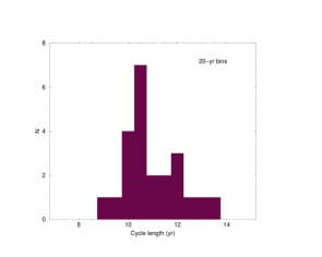
Figure 2: LEFT: The distribution of the solar cycle length does not approach a Dirac function, the ‘quality’ of the cycle only gives values of about 5. RIGHT: The wavelet spectrum of the sunspot-number time series shows two peaks for both 10 yr and 100 yr (Frick et al., 1997a).

2 Basic Theory

Kinematic dynamo theory utilizes only one equation to advance the mean magnetic field in time, i.e.

$$\frac{\partial\langle{\bf B}\rangle}{\partial t}=\mathop{\rm rot}\nolimits\left(\langle{\bf u}\rangle\times\langle{\bf B}\rangle+\mbox{\boldmath$\cal E$}\right).$$ (2)

Here only a non-uniform rotation will be imposed on the mean flow, $\langle{\bf u}\rangle$; any meridional flow shall be introduced later. The turbulent electromotive force (EMF), $\mbox{\boldmath$\cal E$}=\langle{\bf u^{\prime}}\times{\bf B^{\prime}}\rangle$, contains induction $\alpha_{ij}$ and dissipation $\eta_{ijk}$, i.e.

$${\cal E}_{i}=\alpha_{ij}\langle B_{j}\rangle+\eta_{ijk}\langle B_{j}\rangle_{,k}+\dots\ .$$ (3)

Both tensors are pseudo-tensors. While for $\eta_{ijk}$ an elementary isotropic pseudo-tensor exists (“$\varepsilon_{ijk}$”), the same is not true for $\alpha_{ij}$. An odd number of $\Omega$’s is, therefore, required for the $\alpha$-tensor, which is only possible with an odd number of another preferred direction, (say) ${\bf g}$. The $\alpha$-effect can thus only exist in stratified, rotating turbulence. The first formula reflecting this situation,

$$\alpha=c_{\alpha}\frac{l^{2}_{\rm corr}~{}\Omega}{H_{\rho}}\cos{\theta},$$ (4)

was given by Krause (1967) with $\Omega$ being the angular velocity of the basic rotation, $\theta$ the colatitude, and $H_{\rho}$ the density scale height. Evidently, $\alpha$ is a complicated effect, where the effective $\alpha$ might really be very small; the unknown factor $c_{\alpha}$ in (4) may be much smaller than unity. The strength of this effect was computed in recent analytical and numerical simulations for both convectively unstable as well as stable stratifications. While Brandenburg et al. (1990) worked with a box heated from below, Brandenburg and Schmitt (1998) considered magnetic buoyancy in the transition region between the radiative solar core and the convection zone, Brandenburg (2000) probed the Balbus-Hawley instability for dynamo-$\alpha$ production. Ferrière (1993), Kaisig et al. (1993), and Ziegler et al. (1996) used random supernova explosions to drive the galactic turbulence. The magnitudes of the $\alpha$-effects do not reach the given estimate in these cases: the dimensionless factor $c_{\alpha}$ seems really to be much smaller than unity.

2.1 Simple Dynamos

2.1.1 Dynamo waves

An illuminating example of kinematic dynamo theory for the cycle period is the dynamo wave solution. In plane Cartesian geometry there is a mean magnetic field subject to a (strong) shear flow and an $\alpha$-effect – all quantities vary only in the $z$-direction with a given wave number (Parker, 1975). The amplitude equations can then be written as

$$\dot{A}+A=C_{\alpha}B,\ \ \ \dot{B}+B=iC_{\Omega}A,$$ (5)

with $A$ representing the poloidal magnetic field component and $B$ the toroidal component. $C_{\alpha}$ is the normalized $\alpha$ and $C_{\Omega}$ is the normalized shear. The eigenfrequency of the equation system is the complex number

$$\omega_{\rm cyc}=\sqrt{{{\cal D}\over 2}}+i\left(1-\sqrt{{{\cal D}\over 2}}\right).$$ (6)

A marginal solution of the magnetic field is found for a ‘dynamo number’ ${\cal D}\equiv C_{\alpha}C_{\Omega}=2$. In that case the field is not steady but oscillates with the (dimensionless) frequency $\omega_{\rm cyc}=1$.

The (re-normalized) cycle period is thus given simply by combining the eddy diffusivity and the wave number, i.e. $\omega_{\rm cyc}\simeq\eta_{\rm T}k^{2}$ (which is simply the skin-effect relation). With a mixing-length expression for the eddy diffusivity, $\eta_{\rm T}=c_{\eta}l^{2}_{\rm corr}/\tau_{\rm corr}$, one finds the basic relation between the cycle time and the correlation time as

$$\frac{\tau_{\rm cyc}}{\tau_{\rm corr}}=\frac{1}{2\pi c_{\eta}}\left(\frac{R}{l_{\rm corr}}\right)^{2}.$$ (7)

Note that $c_{\eta}\leq 0.3$. The ratio between the global scale, $R$, and the correlation length of the turbulence, $l_{\rm corr}$, determines the cycle time. As this ratio has a minimum value of 10, it is thus no problem to reach a factor of 100 between the cycle period and the correlation time. The rotation period does not enter – it only influences the cycle period in the nonlinear regime (for dynamo numbers exceeding 2). For such numbers the frequency increases – and the cycle time becomes shorter.

2.1.2 Shell dynamo

The simplest assumptions about the $\alpha$-effect and the differential rotation are used in the shell dynamo, i.e.

$$\alpha=\alpha_{0}\cos{\theta},\qquad\qquad\Omega={\rm const.}+\Omega^{\prime}x$$ (8)

for $x_{i}<x<1$ (Roberts, 1972; Roberts and Stix, 1972). Positive $\Omega^{\prime}$ means radial super-rotation and negative $\Omega^{\prime}$ means sub-rotation. The solution with the lowest eigenvalue for the sub-rotation case in a thick shell is a solution with dipolar symmetry, which is, in the vicinity of the bifurcation point, the only stable one (Krause and Meinel, 1988).

The cycle time grows with the linear thickness $D$ of the shell. Compared with the dynamo wave, we find a reduction of (7) by the normalized thickness, $d\leq 0.5$. As long as convection zones of main-sequence stars are considered, that is not too dramatic, but what about rather thin layers like the solar overshoot region? As the cycle period is found to vary linearly with $D$ in similar shell models,

$$\tau_{\rm cyc}\simeq 0.26\ \frac{RD}{\eta_{\rm T}},$$ (9)

the cycle time must become dramatically short in very thin boundary layers.

2.1.3 The dynamo dilemma

The sign of $\alpha$ has been presumed as positive in the northern hemisphere and the differential rotation has been considered unknown (Steenbeck and Krause, 1969) from the early years of dynamo theory. Only sub-rotation – with angular velocity increasing inwards – could then produce a suitable butterfly diagram from the latitudinal migration of the toroidal field. In the other case, e.g. where the surface rotation law is applied in the entire convection zone, one cannot reproduce the migration of the toroidal field towards the equator (Köhler, 1973).

The correct field migration according to the sunspot butterfly diagram is generally produced by a negative dynamo number only, which may be either due to positive $\alpha$ in the northern hemisphere and sub-rotation, or negative $\alpha$ and super-rotation. For all dynamos with super-rotation, however, the phase relation between the radial field component and the toroidal field component is $\langle B_{r}\rangle\langle B_{\phi}\rangle>0$, again disagreeing with the observations (Stix, 1976). The prediction of dynamo theory for the solar differential rotation was thus a clear sub-rotation, $\partial\Omega/\partial r<0$. This prediction contrasts with the results of the helioseismology which revealed sub-rotation only near the poles, whereas near the solar equator there is a super-rotation at the base of the convection zone (Fig. 3).

Agreement with the butterfly diagram shall thus be satisfied by a negative $\alpha$ which can be only explained for the overshoot region. But the phase relation of the field components does then not agree with the known one (Yoshimura, 1976; Parker, 1987; Schlichenmaier and Stix, 1995). With the incorrect phase relation it is even problematic to derive the observed properties of the torsional oscillations (Howard and LaBonte, 1980), which are suggested to arise as a result of the backreaction of the mean-field Lorentz force (Schüssler, 1981; Yoshimura, 1981; Rüdiger et al., 1986; Küker et al., 1996).

In the light of recent developments for dynamos with meridional flow included, there could easily exist a solution of this dynamo dilemma in quite an unexpected way (see Section 4).

2.2 Differential Rotation

The theory of the ‘maintenance’ of differential rotation in convective stellar envelopes might be an instructive detour from dynamo theory. Differential rotation is also turbulence-induced but without the complications due to the magnetic fields. It is certainly unrealistic to expect a solution of the complicated problem of the solar dynamo without an understanding of mean-field hydrodynamics. There is even no hope for the stellar dynamo concept if the internal stellar rotation law cannot be predicted.

The main observational features of the solar differential rotation are

• surface equatorial acceleration of about 30%,

• strong polar sub-rotation and weak equatorial super-rotation,

• reduced equator-pole difference in $\Omega$ at the lower convection-zone boundary.

The characteristic Taylor-Proudman structure in the equatorial region and the characteristic disk-like structure in the polar region are comprised by the results. In the search for stellar surface differential rotation, chromospheric activity has been monitored for more than a decade. Surprisingly enough, there is not yet a very clear picture. For example, the rotation pattern of the solar-type star HD 114710 might easily be reversed compared with that of the Sun (Donahue and Baliunas, 1992).

In close correspondence to dynamo theory we develop the theory of differential rotation in a mean-field formulation starting from the conservation of angular momentum,

$$\frac{\partial}{\partial t}\left(\rho r^{2}\sin^{2}{\theta\Omega}\right)+\frac{\partial}{\partial x_{i}}\left(\rho r\sin{\theta}Q_{i\phi}\right)=0,$$ (10)

where the Reynolds stress $Q_{i\phi}$ derived from the correlation tensor

$$Q_{ij}=\langle u^{\prime}_{i}({\bf x},t)u_{j}^{\prime}({\bf x},t)\rangle$$ (11)

corresponds to the EMF in mean-field electrodynamics.

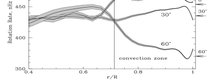
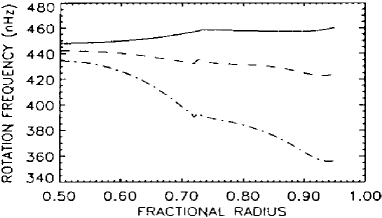
Figure 3: LEFT: The internal rotation of the Sun after the inversion of SOHO data (Kosovichev et al., 1997). RIGHT: Theory of the solar internal rotation by Kitchatinov and Rüdiger (1995). The rotation frequency is given for the equator (solid), mid-latitudes (dashed) and poles (dashed-dotted).

The correlation tensor involves both dissipation (‘eddy viscosity’) as well as ‘induction’ ($\Lambda$-effect):

$$Q_{ij}=\Lambda_{ijk}\Omega_{k}-{\cal N}_{ijkl}\Omega_{k,l}.$$ (12)

Both effects are represented by tensors and must be computed carefully. For anisotropic and rotating turbulence the zonal fluxes of angular momentum can be written as

$$Q_{r\phi} = -\nu_{\perp}r\sin{\theta}\frac{\partial\Omega}{\partial r}-(\nu_{\parallel}-\nu_{\perp})\sin{\theta}\cos{\theta}\left(r\cos{\theta}\frac{\partial\Omega}{\partial r}-\sin{\theta}\frac{\partial\Omega}{\partial\theta}\right)+$$ (13)

$$+ \nu_{\rm T}\left(V^{(0)}+\sin^{2}{\theta V^{(1)}}\right)\Omega\sin{\theta},$$

$$Q_{\theta\phi}=-\nu_{\perp}\sin{\theta}\frac{\partial\Omega}{\partial\theta}-(\nu_{\parallel}-\nu_{\perp})\sin^{2}{\theta}\left(\sin{\theta}\frac{\partial\Omega}{\partial\theta}-r\cos{\theta}\frac{\partial\Omega}{\partial r}\right)+\nu_{\rm T}H^{(1)}\Omega\sin^{2}{\theta}\cos{\theta}$$ (14)

(see Kitchatinov, 1986; Durney, 1989; Rüdiger, 1989). All coefficients are found to be strongly dependent on the Coriolis number

$$\Omega^{*}=2\tau_{\rm corr}~{}\Omega$$ (15)

with $\tau_{\rm corr}$ as the convective turnover time (Gilman, 1992; Kitchatinov and Rüdiger, 1993). Moreover, the most important terms of the $\Lambda$-effect $(V^{(0)},H^{(0)})$ correspond to higher orders of the Coriolis number. The Coriolis number exceeds unity almost everywhere in the convection zone except the surface layers. That is true for all stars – in this sense all main-sequence stars are rapid rotators. Theories linear in $\Omega$ are not appropriate for stellar activity physics. The $\alpha$-effect will thus never run with $\cos{\theta}$ in its first power.

Figure 4: LEFT: The turbulence-originated coefficients in the non-diffusive zonal fluxes of angular momentum in the solar convection zone. $V^{(0)}$ (solid), $V^{(1)}$ (dashed), $V^{(0)}+V^{(1)}$ (dot-dashed). RIGHT: Eddy viscosity in units of $10^{12}$ cm²/s (solid) and Coriolis number $\Omega^{*}$ in the solar convection zone.

The Coriolis number $\Omega^{*}$ is smaller than unity at the top of the convection zone and larger than unity at its bottom. At that depth we find minimal eddy viscosities (‘$\Omega$-quenching’) and maximal $V^{(1)}=H^{(1)}$ (Fig. 4). Since the latter are known as responsible for pole-equator differences in $\Omega$, we can state that the differential rotation is produced in the deeper layers of the convection zone where the rotation must be considered as rapid ($\Omega^{*}\lower 1.72218pt\hbox{$\;\buildrel<\over{\scriptstyle\sim}\;$}10$).

The solution of (10) with the turbulence quantities in Fig. 4 is given in Küker et al. (1993) and Kitchatinov and Rüdiger (1995) using a mixing-length model by Stix and Skaley (1990). With a mixing-length ratio ($\alpha_{\rm MLT}=5/3$) we find the correct equatorial acceleration of about 30 %. There is a clear radial sub-rotation ($\partial\Omega/\partial r<0$) below the poles while in mid-latitudes and below the equator the rotation is basically rigid (right panel in Fig. 3). In this way the bottom value of the pole-equator difference is reduced and the resulting profiles of the internal angular velocity are close to the observed ones. Fig. 5 presents the results of an extension of the theory to a sample of main-sequence stellar models given in Kitchatinov and Rüdiger (1999). Simple scalings like

$${\delta\Omega\over\Omega}\propto\Omega^{\kappa}$$ (16)

may be introduced for both the latitudinal as well as the radial differences of the angular velocity. The $\kappa$-exponents prove to be negative and of order $-1$ (right panel of Fig. 5). So we find that for one and the same spectral type the approximation

$$\delta\Omega\simeq{\rm const.}$$ (17)

should be not too rough. Recent observations of AB Dor (Donati and Cameron, 1997) and PZ Tel (Barnes et al., 1999) seem to confirm this surprising and unexpected result where in all 3 cases the constant value approaches 0.06 day^-1.

Figure 5: The rotation differences $\delta\Omega/\Omega$ for both a solar model and a K5 main-sequence star vs. basic rotation after Kitchatinov and Rüdiger (1999). LEFT: Normalized equator-pole difference of surface rotation, CENTER: The normalized radial differential rotation, RIGHT: The scaling exponent $\kappa$ in (16) for the solar model. In both cases $\kappa\simeq-1$ is approximated.

2.3 The EMF for Turbulence

We now step forward to the turbulent EMF using the same turbulence model as in Section 2.2. We are working with the same quasilinear approximation and the same convection zone model. The additional equation for the magnetic fluctuations is

$${\partial{\bf B}^{\prime}\over\partial t}-\eta_{\rm t}\Delta{\bf B}^{\prime}=\mathop{\rm rot}\nolimits({\bf u}^{\prime}\times\langle{\bf B}\rangle),$$ (18)

where $\eta_{\rm t}\simeq\nu_{\rm t}$ is the small-scale diffusivity. In this configuration we deal with an $\alpha$-tensor being highly anisotropic, even for the most simple case of slow rotation ($\Omega^{*}\ll 1$),

$$\alpha_{ij}=\ \gamma\varepsilon_{ijk}G_{k}-\alpha_{1}({\bf G\Omega})\delta_{ij}-\alpha_{2}(G_{i}\Omega_{j}+G_{j}\Omega_{i})+\ \hat{\gamma}\varepsilon_{ijk}U_{k}-\hat{\alpha}_{1}({\bf U\Omega})\delta_{ij}-\hat{\alpha}_{2}(U_{i}\Omega_{j}+U_{j}\Omega_{i})$$ (19)

(Moffatt, 1978; Krause and Rädler, 1980; Wälder et al., 1980) with the stratification vectors ${\bf G}=\nabla\log\rho$ and ${\bf U}=\nabla\log u_{\rm T}$ with the rms velocity $u_{\rm T}=\sqrt{\langle{\bf u}^{\prime 2}\rangle}$. The $\gamma$-terms describe advection effects, such as turbulent diamagnetism (Rädler, 1968; Kitchatinov and Rüdiger, 1992) and buoyancy (Kitchatinov and Pipin, 1993) and cover the off-diagonal elements of the $\alpha$-tensor.

The diagonal elements are essential for the induction. The mixing-length approximation used in Rüdiger and Kitchatinov (1993) leads to

$$\alpha_{rr}=\hat{\alpha}\left({\bf U}+\frac{\bf G}{4}\right){\bf\Omega},\qquad\qquad\alpha_{\phi\phi}=\alpha_{\theta\theta}=-\hat{\alpha}\left({\bf U}+\frac{3{\bf G}}{2}\right){\bf\Omega}.$$ (20)

While the most important component $\alpha_{\phi\phi}$ becomes positive (if density stratification dominates), the component $\alpha_{rr}$ becomes negative in the northern hemisphere. In contrast to the standard formulation, the $\alpha_{2}$-components in (19) are dominant as confirmed by numerical simulations by Brandenburg et al. (1990). Our quasilinear theory of the $\alpha$-effect provides $\hat{\alpha}=8/15\ \tau_{\rm corr}^{2}u_{\rm T}^{2}$.

The general case of an arbitrary rotation rate is not easy to present. The ‘overshoot’ region, however, is of particular interest and is characterized by $|{\bf U}|>|{\bf G}|$ and $\Omega^{*}\gg 1$. In cylindrical coordinates ($s,\phi,z$) and for very fast rotation one gets

$$\alpha=c_{\alpha}\ \ \left(\matrix{-{3\pi\over 8}\cos\theta&{3\pi\over 8\Omega^{*}}\cos\theta&0\cr-{3\pi\over 8\Omega^{*}}\cos\theta&-{3\pi\over 8}\cos\theta&0\cr 0&-{3\pi\over 8\Omega^{*}}\sin\theta&0\cr}\right)\ \ \frac{d}{dr}\left(\tau_{\rm corr}u_{\rm T}^{2}\right)$$ (21)

(Rüdiger  and Kitchatinov, 1993). Note that

• all components with index $z$ disappear,

• the remaining diagonal terms (the $\alpha$-effect) do not vanish for very rapid rotation,

• the $\alpha$-terms are negative (in the northern hemisphere) for outward increase of the turbulence intensity (like in the overshoot region),

• the advection terms tend to vanish for rapid rotation; their relation to the $\alpha$-effect is given by the Coriolis number $\Omega^{*}$.

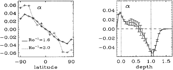
Figure 6: Simulation of the $\alpha$-effect after Brandenburg (1994b) versus latitude and depth. Note the negative values at the bottom of the convection zone (RIGHT) and the maximum for high latitudes (LEFT).

It might seem that the $\alpha$-effect is now in our hands. There are, however, shortcomings beyond the use of the quasilinear approximation. The main point is the absence of terms higher than first order in ${\bf G}$ or ${\bf U}$, respectively. In particular, all terms with (${\bf G\Omega})^{3}\sim\cos^{3}{\theta}$ are missing so that we have no information about the $\alpha$-effect at the poles where for slow rotation $\alpha_{\phi\phi}$ is largest. However, this need not to be true for ‘rapid’ rotation. Simulations of $\alpha_{\phi\phi}$ with its latitudinal profile by Brandenburg (1994b) indeed showed that the maximum occurs at mid-latitudes (Fig. 6). Schmitt (1985, 1987) derived a similar profile for a different type of instability.

A new discussion of the $\alpha$-effect in shear flows recently emerged (cf. Brandenburg and Schmitt, 1998). A quasilinear computation of the influence of the differential rotation on the $\alpha$-effect leads to

$$\alpha\simeq-l_{\rm corr}^{2}{\partial\Omega\over\partial\theta}{d\log(\rho u_{\rm T})\over dr}\sin\theta$$ (22)

for a sphere or

$$\alpha\simeq-l_{\rm corr}^{2}\ s{d\Omega\over ds}{d\log\rho\over dz}$$ (23)

for a disk (Rüdiger and Pipin, 2000). The latter relation for accretion disks with $\partial\Omega/\partial s<0$ yields negative $\alpha$-values in the northern hemisphere and positive values in the southern hemisphere (see Brandenburg and Donner, 1997). According to (21) or (22), negative values for the northern $\alpha_{\phi\phi}$ in the solar overshoot region are only achievable with a very steep decrease of the turbulence intensity with depth.

There are very interesting observational issues concerning the current helicity

$${\cal H}_{\rm curr}=\langle\mbox{\boldmath$j$}^{\prime}\cdot\mbox{\boldmath$B$}^{\prime}\rangle$$ (24)

with the electric current $\mbox{\boldmath$j$}=\mathop{\rm rot}\nolimits\mbox{\boldmath$B$}/\mu_{0}$. The current helicity has the same kind of equatorial (anti-) symmetry as the dynamo-$\alpha$. For homogeneous global magnetic fields, the dynamo-$\alpha$ is related to the turbulent EMF according to $\alpha_{ij}\bar{B}_{i}\bar{B}_{j}={\mbox{\boldmath$\cal E$}}\cdot\bar{\mbox{\boldmath$B$}}$. After Rädler and Seehafer (1990) we read this equation as $\alpha_{\phi\phi}={\mbox{\boldmath$\cal E$}}\cdot\bar{\mbox{\boldmath$B$}}/\bar{B}_{\phi}^{2}$, where $\alpha_{\phi\phi}$ is the dominant component of the $\alpha$-tensor. We are, in particular, interested in checking their and Keinigs’ (1983) antiphase relation,

$${\alpha_{\phi\phi}\bar{B}^{2}\over\mu_{0}{\cal H}_{\rm curr}}=-\eta<0,$$ (25)

between $\alpha$-effect and current helicity. In addition, we have recently shown that indeed the negativity of the left-hand-side of (25) is preserved for magnetic-driven turbulence fields which do not fulfill the conditions for which the Keinigs relation (25) originally has been derived (Rüdiger et al., 2000).

An increasing number of papers presents observations of the current helicity at the solar surface, all showing that it is negative in the northern hemisphere and positive in the southern hemisphere (Hale, 1927; Seehafer, 1990; Pevtsov et al., 1995; Abramenko et al., 1996; Bao and Zhang, 1998; see Low (1996) for a review). There is thus a strong empirical evidence that the $\alpha$-effect is positive in the bulk of the solar convection zone in the northern hemisphere.

For a given field of magnetic fluctuations the dynamo-$\alpha$  as well as the kinetic and current helicities, have been computed by Rüdiger et al.  (2000) assuming that the turbulence is subject to magnetic buoyancy and global rotation. In particular, the role of magnetic buoyancy appears quite important for the generation of $\alpha$-effect. So far, only the role of density stratification has been discussed for both $\alpha$-effect and $\Lambda$-effect, and their relation to kinetic helicity and turbulence anisotropy. If density fluctuations shall be included then it makes no sense here to adopt the anelastic approximation $\mathop{\rm div}\nolimits\rho\mbox{\boldmath$u$}^{\prime}=0$ but one has to work with the mass conservation law in the form

$${\partial\rho^{\prime}\over\partial t}+\bar{\rho}\mathop{\rm div}\nolimits\mbox{\boldmath$u$}^{\prime}=0.$$ (26)

For the turbulent energy equation one can simply adopt the polytropic relation $p^{\prime}=c_{\rm ac}^{2}\rho^{\prime},$ where $c_{\rm ac}$ is the isothermal speed of sound. The turbulence is thus assumed to be driven by the Lorentz force and it is subject to a global rotation. The result is an $\alpha$-effect of the form

$$\alpha_{\phi\phi}=-{1\over 5}{\tau_{\rm corr}^{2}\over c_{\rm ac}^{2}}{\langle{B^{(0)}}^{2}\rangle\over\mu_{0}\rho}(\mbox{\boldmath$g$}\cdot\mbox{\boldmath$\Omega$}).$$ (27)

Here $g$ is the gravitional acceleration, and the energy of the magnetic fluctuations forcing the turbulence is also given. For rigid rotation the $\alpha$-effect proves thus to be positive in the northern hemisphere and negative in the southern hemisphere. Again we do not find any possibility to present a negative $\alpha$-effect in the northern hemisphere.

The kinetic helicity

$${\cal H}_{\rm kin}=\langle\mbox{\boldmath$u$}^{\prime}\cdot\mathop{\rm rot}\nolimits\mbox{\boldmath$u$}^{\prime}\rangle$$ (28)

has just the same latitudinal distribution as the $\alpha$-effect, but the magnetic model does not provide the minus sign between the dynamo-$\alpha$ and the kinetic helicity which is characteristic within the conventional framework, $\alpha\propto-\tau_{\rm corr}\ {\cal H}_{\rm kin}$. If a rising eddy can expand in density-reduced surroundings, then a negative value of the kinetic helicity is expected. The magnetic-buoyancy model, however, leads to another result.

If the real convection zone turbulence is formed by a mixture of both dynamic-driven and magnetic driven turbulence, the kinetic helicity should also be a mixture of positive parts and negative parts so that it should be a rather small quantity. The opposite is true for the current helicity which also changes its sign at the equator. Again it turns out to be negative in the northern hemisphere and positive in the southern hemisphere. The current helicity (due to fluctuations) and the $\alpha$-effect are thus always out of phase. The current helicity at the solar surface might thus be considered a much more robust observational feature than the kinetic helicity (28).

Strong magnetic fields are known to suppress turbulence and the $\alpha$-effect is also expected to decrease. The field strength at which the $\alpha$-effect reduces significantly is assumed, in energy, to be comparable with the kinetic energy of the velocity fluctuations, and is called the equipartition field strength $B_{\rm eq}=\left(\mu_{0}\rho u_{\rm T}^{2}\right)^{1\!/\!2}$. The magnetic feedback on the turbulence was studied by Rüdiger & Kitchatinov (1993) using a $\delta$-function spectral distribution of velocity fluctuations. The $\alpha_{\phi\phi}$-component of the $\alpha$-tensor acting in an $\alpha\Omega$-dynamo is found to be suppressed by the magnetic field with the $\alpha$-quenching function

$$\Psi=\frac{15}{32\beta^{4}}\left(1-\frac{4\beta^{2}}{3(1+\beta^{2})^{2}}-\frac{1-\beta^{2}}{\beta}\arctan\beta\right)$$ (29)

with

$$\beta=|\langle B\rangle|/B_{\rm eq}.$$ (30)

The quenching function decreases as $\beta^{-3}$ for strong magnetic fields. The function is similar to the heuristic approach $(1+\beta^{2})^{-1}$ which is artificial but nevertheless frequently used in $\alpha$-effect dynamos. For small fields, $\Psi$ runs like $1-\frac{12}{7}\beta^{2}$, the mentioned heuristic approximation runs like $1-\beta^{2}$.

We can also compute the eddy diffusivity using the same turbulence theory as in the previous Section. The simplest expression is

$$\eta_{\rm T}=\ c_{\eta}\tau_{\rm corr}u_{\rm T}^{2}$$ (31)

with $c_{\eta}\lower 1.72218pt\hbox{$\;\buildrel<\over{\scriptstyle\sim}\;$}0.3$. This expression, however, fails to include rotation and stratification. Even a non-uniform but weak magnetic field induces a turbulent EMF, without rotation and stratification in accordance to $\eta_{ijk}=\eta_{\rm T}\varepsilon_{ijk}$. A much stronger ‘magnetic quenching’ of such an eddy diffusivity has been discussed by Vainshtein and Cattaneo (1992) and Brandenburg (1994a) and is still a matter of debate. A more conventional theory of the $\eta_{\rm T}$-quenching and its consequences for the stellar activity cycle theory is given in Section 6 below.

3 A Boundary-Layer Dynamo for the Sun

The spatial location of the dynamo action is unknown unless helioseismology will reveal the exact position of the magnetic toroidal belts beneath the solar surface (cf. Dziembowski and Goode, 1991). There are, however, one or two arguments in favour of locating it deep within or below the convection zone:

• Hale’s law of sunspot parities can only be fulfilled if the toroidal magnetic field belts are very strong (10⁵ Gauss, see Moreno-Insertis, 1983; Choudhuri, 1989; Fan et al., 1993; Caligari et al., 1995).

• The dynamo field strength is approximately the equipartition value $B_{\rm eq}=\left(\mu_{0}\rho u_{\rm T}^{2}\right)^{1\!/\!2}$. Using mixing-length theory arguments $\rho u_{\rm T}^{3}\simeq\$const., hence $B_{\rm eq}$ is increasing inwards with $\rho^{1/6}$ (one order of magnitude, $\lower 1.72218pt\hbox{$\;\buildrel<\over{\scriptstyle\sim}\;$}10^{4}$ Gauss).

• The radial gradient of $\Omega$ is maximal below the convection zone.

As a consequence of these arguments high field amplitudes might be generated only in the layer between the convection zone and the radiative interior (Boundary layer (BL), ‘tachocline’, see van Ballegooijen, 1982). On the other hand, if there is some form of ‘turbulence’ in this layer, it will be hard to understand the present-day finite value of lithium in the solar convection zone. The lithium burning only starts 40 000 km below the bottom of the convection zone. Any turbulence in this domain would lead to a rapid and complete depletion of the lithium in the convection zone, which is not observed. Moreover, as shown by Rüdiger and Kitchatinov (1997), it is also not easy to generate very strong toroidal magnetic fields in the solar tachocline as the Maxwell stress tends to deform the rotation profile to more and more smooth functions. In our computation with molecular diffusion coefficient values the toroidal field amplitude never did exceed 1 kGauss, independent of the radial magnetic field applied.

Krivodubskij and Schultz (1993) (with the inclusion of the depth-dependence of the Coriolis number $\Omega^{*}$ and using a mixing-length model) derived a profile of the $\alpha$-effect (Fig. 7) with a magnitude of 100 m/s, positive in the convection zone and negative in the overshoot layer. The negativity of $\alpha$ there can only be relevant for the dynamo if the bulk of the convection zone is free from $\alpha$. It has been argued that the short rise-times of the flux tubes in the convection zone prevent the formation of the $\alpha$-effect (Spiegel and Weiss, 1980; Schüssler, 1987; Stix, 1991). However, the rise-times may be much longer in the overshoot region (Ferriz-Mas and Schüssler, 1993, 1995; van Ballegooijen, 1998). Anyway, as $C_{\alpha}=1$ is used in Fig. 7, the given values can only be considered as maximal values.

Figure 7: The depth-dependence of the $\alpha$-effect with $C_{\alpha}=1$. Note the different contributions by density gradient and turbulence intensity distribution. The $\alpha$-effect becomes negative only at the bottom of the convection zone (Krivodubskij and Schultz, 1993).

There is a serious shortcoming of the BL concept. The characteristic scales of the magnetic fields are no longer much larger than the scales of the turbulence. The validity of the local formulations of the mean-field electrodynamics is not ensured for such thin layers. Nevertheless, there is an increasing number of corresponding quantitative models (Choudhuri, 1990; Belvedere et al., 1991; Prautzsch, 1993; Markiel and Thomas, 1999). Even in this case a couple of new questions will arise. For a demonstration of this puzzling situation a model has been established by Rüdiger and Brandenburg  (1995) under the following assumptions:

• Intermittency (or the weakness of the turbulence in the BL) is introduced by a dilution factor $\epsilon$ in ${\cal E}_{i}=\epsilon\ (\alpha_{ij}\langle B_{j}\rangle+\eta_{ijk}\langle B_{j}\rangle_{,k})$. The factor $\epsilon$ controls the weight of the turbulent EMF in relation to the differential rotation.

• The ignorance of the $\alpha$-effect in the polar regions is parameterized with  $\alpha_{\rm u}$  with  $\alpha\sim\alpha_{\rm u}\,\cos\theta\sin^{2}\theta$.

• $\alpha$ exists only in the overshoot region, $\eta_{\rm T}$ only in the convection zone.

• The correlation time is taken from $\tau_{\rm corr}\simeq D/u_{\rm T}\simeq 10^{6}$ s so that $\Omega^{*}\simeq$ 5 results.

• The tensors $\alpha$ and $\eta_{\rm T}$ are computed for a rms velocity profile by Stix (1991), the rotation law is directly taken from Christensen-Dalsgaard and Schou (1988).

The main results from these models are:

• The cycle period has just the same sensitivity to the BL’s thickness as the shell dynamo, i.e.   $\tau_{\rm cyc}$[yr] $\sim D/\epsilon$ for $D$ in Mm ($D\simeq$ 15…35 Mm).

• Due to the rotational $\eta_{\rm T}$-quenching the linear model yields the correct cycle time. Generally the 22-year cycle can only exist for a dilution of $\epsilon\simeq 0.5$ (cf. Fig. 8).

• For $\alpha_{\rm u}\simeq 0$ the magnetic activity is concentrated near the poles, for $\alpha_{\rm u}\simeq 1$ it moves to the equator.

• For too thin BL’s there are too many toroidal magnetic belts in each hemisphere (Fig. 9).

Figure 8: Cycle period $\tau_{\rm cyc}$ as a function of the BL thickness $D/R$ and and the dilution factor $\epsilon$ for $\alpha_{\rm u}=0$. LEFT: $\epsilon=0.5$, the results are well represented by $\tau_{\rm cyc}=D\,$[yr/Mm]. RIGHT: $D=35$ Mm. The horizontal line indicates the solar cycle period of 22 years.

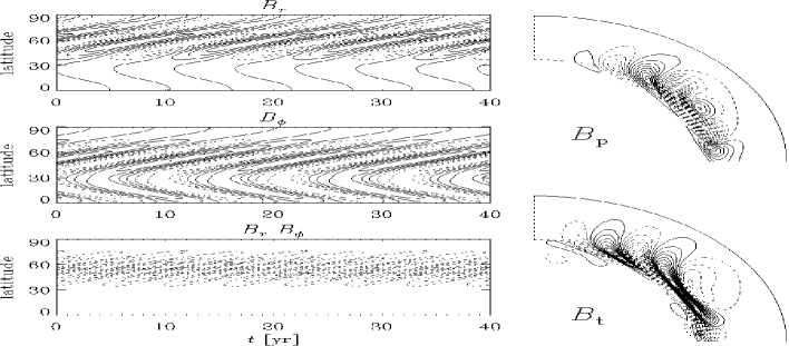
Figure 9: The magnetic field geometry for the nonlinear ($\alpha$-quenched) solution without buoyancy and $\epsilon=0.5$, $D=35$ Mm, $\alpha_{\rm u}=1$. An obvious problem of the BL dynamo is the large number of toroidal field belts.

The dependence of the cycle period on $\epsilon$ is shown in Fig. 8. For $\epsilon\approx 1$ the linear solutions have the correct 22-year solar cycle period (right panel). The cycle period increases linearly with $D$,

$$\tau_{\rm cyc}\propto D,$$ (32)

(see left panel of Fig. 8), which is in agreement with the linear relation (9) for spherical shell dynamos. For too thin boundary layers the cycle time will thus become very short. Nonlinearity further shortens the cycle period and this effect has to be compensated for by taking a smaller value of $\epsilon$, depending on whether or not magnetic buoyancy is included.

In those cases where $\alpha$-quenching and magnetic buoyancy are included, the rms-values of the poloidal and toroidal fields are 11 Gauss and 5 kGauss. Poloidal and toroidal fields as well as their mean and fluctuating parts are difficult to disentangle observationally. A toroidal field of 5 kGauss is, however, consistent with the observed total flux of $10^{24}$ Mx, distributed over 50 Mm in depth and 400 Mm in latitude. On the other hand, a poloidal field of 11 Gauss is larger than the observed value.

In all cases the magnetic field exceeds the equipartition value which is here 6 kGauss. This is partly due to the turbulent diamagnetism leading to an accumulation of magnetic fields at the bottom of the convection zone, and partly due to too optimistic estimates for $\alpha$-quenching.

The dilution factor $\epsilon$ is the main free parameter that must be chosen such that the 22-year magnetic cycle period is obtained. The thickness of the overshoot layer must be chosen to match the correct number of toroidal field belts of the Sun. Our results suggest that the thickness should not be much smaller than $D\approx 35\,$Mm$\,\approx 1/2H_{p}$.

Nonlinear effects typically lead to a reduction of the magnetic cycle period. Unfortunately, there are no consistent quenching expressions that are valid for rapid rotation. Magnetic buoyancy also provides a nonlinear feedback (e.g. Durney and Robinson, 1982; Moss et al., 1990), but computations by Kitchatinov and Pipin (1993) indicate that this only leads to a mean field advection of a few m/s, i.e. less than the advection due to the diamagnetic effect. However, magnetic buoyancy is important in the upper layers (where the diamagnetic effect is weak), and can have significant effects on the field geometry and the cycle period (Kitchatinov, 1993).

4 Distributed Dynamos with Meridional Circulation

Not only differential rotation but also meridional flow $u^{\rm m}$ will influence the mean-field dynamo. This influence can be expected to be only a small modification if and only if its characteristic time scale $\tau_{\rm drift}$ exceeds the cycle time $\tau_{\rm cyc}$ of about 11 years. With $\tau_{\rm drift}\simeq R/u^{\rm m}$ we find $u^{\rm m}\simeq$ 2 m/s as a critical value. If the flow is faster (Fig. 10) the modification can be drastic. In particular, if the flow counteracts the diffusion wave, i.e. if the drift at the bottom of the convection zone is polewards, the dynamo might come into trouble. The behaviour of such a solar-type dynamo (with superrotation at the bottom of the convection zone and perfect conduction beneath the convection zone) is demonstrated in the present Section.

Figure 10: The meridional circulation at mid-latitudes (45^∘) at the bottom (LEFT) and the top (RIGHT) of the convection zone for both a solar model and a K5 main-sequence star as a function of rotation period (Kitchatinov and Rüdiger, 1999). The circle represents the solar case. The flow at the bottom is equatorwards (as it is the flow at the surface, there are 2 cells in radius).

In the following the dynamo equations are given with the inclusion of the induction by meridional circulation. For axisymmetry the mean flow in spherical coordinates is given by ${\bf u}=\left(u_{r},u_{\theta},r\sin\theta\ \Omega\right)$.

With a similar notation the magnetic field is

$${\bf B}=\left({1\over r^{2}\sin\theta}{\partial A\over\partial\theta},-{1\over r\sin\theta}{\partial A\over\partial r}\ ,\ B\right)$$ (33)

with $A$ as the poloidal-field potential and $B$ as the toroidal field. Their evolution is described by

$${\partial A\over\partial t}+({\bf u}\cdot\nabla)A = \alpha sB+\eta_{\rm T}\left({\partial^{2}A\over\partial r^{2}}+{\sin\theta\over r^{2}}{\partial\over\partial\theta}\left({1\over\sin\theta}{\partial A\over\partial\theta}\right)\right),$$ (34)

$${\partial B\over\partial t}+s\rho({\bf u}\cdot\nabla){B\over{s\rho}} = {1\over r}\left({\partial\Omega\over\partial r}{\partial A\over\partial\theta}-{\partial\Omega\over\partial\theta}{\partial A\over\partial r}\right)-{1\over s}{\partial\over\partial r}\left(\alpha{\partial A\over\partial r}\right)-{1\over r^{3}}{\partial\over\partial\theta}\left({\alpha\over\sin\theta}{\partial A\over\partial\theta}\right)+$$ (35)

$$+ {\eta_{\rm T}\over s}\left({\partial^{2}(sB)\over\partial r^{2}}+{\sin\theta\over r}{\partial\over\partial\theta}\left({1\over s}{\partial(sB)\over\partial\theta}\right)\right)$$

for uniform $\eta_{\rm T}$ and with $s=r\sin\theta$ (cf. Choudhuri et al., 1995). In order to produce here a solar-type butterfly diagram with ${\bf u}=0$ the $\alpha$-effect must be taken as negative in the northern hemisphere (Steenbeck and Krause, 1969; Parker, 1987). Our rotation law and the radial meridional flow profile at 45^∘ are given in Fig. 11. A one-cell flow pattern is adopted in each hemisphere. The $u^{\rm m}$ approximates the latitudinal drift close to the convection zone bottom, the circulation is counterclockwise (in the first quadrant) for positive $u^{\rm m}$, i.e. towards the equator at the bottom of the convection zone.

Figure 11: Rotation law and the pattern of a meridional flow at 45^∘ for the Steenbeck-Krause dynamo model of Section 4. The meridional circulation is prescribed (Rüdiger, 1989) and not yet a result of differential rotation theory. The rotation profile always has a positive slope.

Note that the cycle period becomes shorter for clockwise flow (Roberts and Stix, 1972) and it becomes longer for the more realistic counterclockwise flow. The latter forms a poleward flow at the surface in agreement with observations and theory (Fig. 10). For too strong meridional circulation ($u^{\rm m}\geq 50$ m/s) our dynamo stops operation. The same happens already for $u^{\rm m}\approx-$ 10 m/s if the flow at the bottom is opposite to the magnetic drift wave.

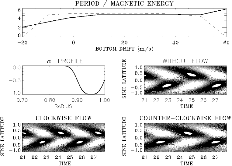
Figure 12: Operation of a Steenbeck-Krause dynamo with negative alpha-effect (in northern hemisphere) with and without meridional circulation. Eddy diffusivity is $5\cdot 10^{12}\ {\rm cm}^{2}/{\rm s}$. Positive bottom drift means counterclockwise flow (equatorwards at the bottom of the convection zone, polewards at the surface). TOP: The cycle period (solid, in years) and the magnetic energy (dashed) vs. the latitudinal drift at the bottom of the convection zone. MIDDLE: $\alpha$-profile in radius and butterfly diagram of the circulation-free dynamo. The maximal toroidal field is plotted vs. the time in years. BOTTOM: Butterfly diagrams for clockwise and counterclockwise circulations.

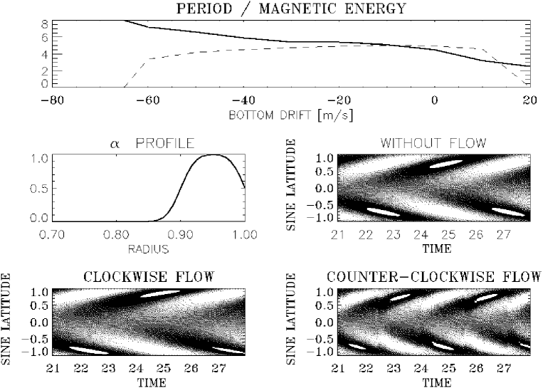
Figure 13: The same as in Fig. 12 but for positive $\alpha$-effect (in northern hemisphere). Note the decay of the dynamo already for 10…20 m/s (equatorwards at the bottom, polewards at the top of the convection zone).

However, it is hard to explain why the convection zone itself is producing the negative $\alpha$-values used in the model. More easy to understand are the positive values adopted in Fig. 13 (see Durney 1995, 1996). Of course, now without circulation the butterfly diagram becomes ‘wrong’, with a poleward migration of the toroidal magnetic belts. One can also understand that the counterclockwise flow (equatorwards at the convection zone bottom) rapidly destroys the dynamo operation, here already for 10 m/s amplitude. This amplitude is so small that it cannot be a surprise that such a dynamo might not be realized in the Sun. For the eddy diffusivity $5\cdot 10^{12}$ cm²/s is used here, so the magnetic Reynolds number ${\rm Rm}=u^{\rm m}R/\eta_{\rm T}$ is

$${\rm Rm}=14\ {u^{\rm m}\over 10\ {\rm m/s}},$$ (36)

i.e. ${\rm Rm}=14$ for $u^{\rm m}=10$ m/s. In their paper Choudhuri et al. (1995) apply Reynolds numbers of order 500 while Dikpati and Charbonneau (1999) even take ${\rm Rm}=1400$. Indeed, their dynamos are far beyond the critical values of ${\rm Rm}\simeq 10$ which are allowed for the weak-circulation $\alpha\Omega$-dynamo. Their dynamos exhibit the same period reduction for increasing $u^{\rm m}$ shown in Fig. 13 but the butterfly diagram is opposite. It seems that quite another branch of dynamos would exist for ${\rm Rm}\gg 10$. This is indeed true.

Table 1: Cycle periods in years of solar-type-butterfly dynamos (bold) with positive $\alpha$-effect (= 3 m/s) and meridional flow of $u^{\rm m}$ at the bottom of the convection zone, the eddy diffusivity given in the headline. Signature ‘$-$’ indicates polewards migration, ‘decay’ means decaying fields. Note the good representation of the $\eta$-dependence of the cycle time of (9) in the first line of the Table.

$u^{\rm m}$ [m/s]	$1\cdot 10^{11}$ cm2/s	$2\cdot 10^{11}$ cm2/s	$5\cdot 10^{11}$ cm2/s
1	$-$120	$-$70	$-$36
3	$-$160	$-$45	$-$24
5	$-$145	$-$40	decay
7	$-$131	$-$26	decay
11	$-$120	$-$20	decay

The butterfly diagram of such a dynamo with positive $\alpha$-effect (3 m/s) and a magnetic Reynolds number of 450 is given in Fig. 14. It works with low eddy diffusivity of $10^{11}\ {\rm cm}^{2}/{\rm s}$ and the flow pattern of Fig. 11. In the lower panel the phase relation of poloidal and toroidal magnetic fields is shown. In lower latitudes the observed phase lay between the field components is obtained. In Table 1 the cycle periods in years are given for positive-$\alpha$ dynamos. Bold numbers indicate the solar-type butterfly diagram. For fast meridional flow and small eddy diffusivity we indeed find oscillating dynamos. The eddy diffusivity is the same as that known from the sunspot decay, i.e. $10^{11}$ cm²/s (see Brandenburg, 1993).

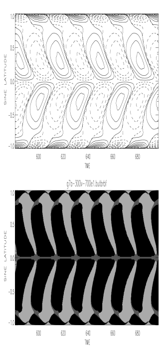
Figure 14: TOP: Butterfly diagram of a marginal dynamo with positive $\alpha$-effect (3 m/s), with eddy diffusivity of $10^{11}$ cm²/s and a bottom flow of 7 m/s. BOTTOM: $\langle B_{r}\rangle\langle B_{\phi}\rangle$, black colour indicates negative sign, i.e. the observed phase lay between poloidal and toroidal field.

5 The Maunder Minimum

The period of the solar cycle and its amplitude are far from constant. The most prominent activity drop was the Maunder minimum between 1670 and 1715 (Spörer, 1887). The variability of the cycle period can be expressed by the ‘quality’, $\omega_{\rm cyc}/\Delta\omega_{\rm cyc}$, which is as low as 5 for the Sun (Hoyng, 1993, cf. Fig. 2).

Measurements of ¹⁴C abundances in sediments and long-lived trees provide much longer time series than sunspot counts. In agreement with Schwarz (1994), Vos et al. (1996, 1997) found a secular periodicity of 80–90 years as well as a long-duration period of about 210 years. The measurements of atmospheric ¹⁴C abundances by Hood and Jirikowic (1990) suggested a periodicity of 2400 years which is also associated with a long-term variation of solar activity. The variety of frequencies found in solar activity may even indicate chaotic behaviour as discussed by Rozelot (1995), Kurths et al. (1993, 1997) and Knobloch and Landsberg (1996).

The activity cycle of the Sun is not exceptional: The observation of chromospheric Ca-emission of solar-type stars yields activity periods between 3 and 20 years (Noyes et al., 1984; Baliunas and Vaughan, 1985; Saar and Baliunas, 1992a,b). A few of these stars do not show any significant activity. This suggests that even the existence of the grand minima is a typical property of cool main-sequence stars like the Sun. From ROSAT X-ray data Hempelmann et al. (1996) find that up to 70% of the stars with a constant level of activity exhibit a rather low level of coronal X-ray emission. HD 142373 with its X-ray luminosity of only $\log F_{\rm X}=3.8$ is a typical candidate. We conclude that during a grand minimum not only the magnetic field in the activity belts is weaker than usual but the total magnetic field energy is also reduced.

The short-term cycle period appears to decrease at the end of a grand minimum according to a wavelet analysis of sunspot data by Frick et al. (1997). There is even empirical evidence for a very weak but persistent cycle throughout the solar Maunder minimum as found by Wittmann (1978) and recently Beer et al. (1998). The latitudinal distribution of the few sunspots observed during the Maunder minimum was highly asymmetric (Spörer, 1887; Ribes and Nesme-Ribes, 1993; Nesme-Ribes et al., 1994). Short-term deviations from the north-south symmetry in regular solar activity are readily observable (Verma, 1993), yet a 30-year period of asymmetry in sunspot positions as seen during the Maunder minimum remains a unique property of grand minima and should be associated with a parity change of the internal magnetic fields.

5.1 Mean-field Magnetohydrodynamics

The explanation of grand minima in the magnetic activity cycle by a dynamo action has been approached by two concepts. The first one considers the stochastic character of the turbulence and studies its consequences for the variations of the $\alpha$-effect and all related phenomena with time (see Section 8). The alternative concept includes the magnetic feedback to the internal solar rotation (Weiss et al., 1984; Jennings and Weiss, 1991). Kitchatinov et al. (1994a) and Tobias (1996, 1997) even introduced the conservation law of angular momentum in the convection zone including magnetic feedback in order to simulate the intermittency of the dynamo cycle.

A theory of differential rotation based on the $\Lambda$-effect concept is coupled with the induction equation in a spherical 2D mean-field model. The mean-field equations for the convection zone include the effects of diffusion, $\alpha$-effect, toroidal field production by differential rotation and the Lorentz force. They are

$${\partial A\over\partial t}=\eta_{\rm T}{\partial^{2}A\over\partial r^{2}}+\eta_{\rm T}{\sin\theta\over r^{2}}{\partial\over\partial\theta}\left({1\over\sin\theta}{\partial A\over\partial\theta}\right)+\alpha r\sin\theta B,$$ (37)

$${\partial B\over\partial t} = {1\over r}{\partial\over\partial r}\left(\eta_{\rm T}{\partial(Br)\over\partial r}\right)+{\eta_{\rm T}\over r^{2}}{\partial\over\partial\theta}\bigg{(}{1\over\sin\theta}{\partial(B\sin\theta)\over\partial\theta}\bigg{)}+$$ (38)

$$+ {1\over r}{\partial\Omega\over\partial r}{\partial A\over\partial\theta}-{1\over r}{\partial\Omega\over\partial\theta}{\partial A\over\partial r}-{1\over r\sin\theta}\ {\partial\over\partial r}\left(\alpha\ {\partial A\over\partial r}\right)-{1\over r^{3}}\ {\partial\over\partial\theta}\left({\alpha\over\sin\theta}\ {\partial A\over\partial\theta}\right),$$

$$\rho r\sin\theta{\partial\Omega\over\partial t}=-{1\over r^{3}}{\partial\over\partial r}\left(r^{3}\rho\ Q_{r\phi}\right)-{1\over r\sin^{2}\theta}{\partial\over\partial\theta}\left(\sin^{2}\theta\rho\ Q_{\theta\phi}\right)+$$ (39)

$$+{1\over\mu_{0}r^{2}\sin\theta}\bigg{(}{1\over r}{\partial A\over\partial\theta}{\partial(Br)\over\partial r}-{1\over\sin\theta}{\partial A\over\partial r}{\partial(B\sin\theta)\over\partial\theta}\bigg{)}.$$

Since the importance of the large-scale Lorentz force in the momentum equation was discussed by Malkus and Proctor (1975), we call this term ‘Malkus-Proctor’ effect.

The computational domain is a spherical shell covering the outer parts of the Sun down to a fractional solar radius, $x=r/R$, of $0.5$. The convection zone extends from $x=0.7$ to $x=1$. The $\alpha$-effect works only in the lower part from $x=0.7$ to $x=0.8$ while turbulent diffusion of the magnetic field, turbulent viscosity, and the $\Lambda$-effect are present in the entire convection zone. Below $x=0.7$ both the magnetic diffusivity and the viscosity are two orders of magnitude smaller than in the convection zone. The boundary conditions are specified as $Q_{r\phi}=\partial A/\partial r=B=0\qquad{\rm at}\ \ r=R$, and $Q_{r\phi}=A=B=0$ at the inner boundary. The angular momentum flux is given by

$$Q_{r\phi}=\nu_{\rm T}\ \sin\theta\left(-r\ {\partial\Omega\over\partial r}+V^{(0)}\Omega\right),\qquad Q_{\theta\phi}=-\nu_{\rm T}\ \sin\theta\ {\partial\Omega\over\partial\theta}.$$ (40)

$V^{(0)}$ determines the radial rotation law without magnetic field.

Five dimensionless numbers define the model, namely the magnetic Reynolds numbers of both the differential rotation and the $\alpha$-effect, $C_{\Omega}=\Omega_{0}R^{2}/\eta_{\rm T}$, $C_{\alpha}=\alpha_{0}R/\eta_{\rm T}$; the magnetic Prandtl number ${\rm Pm}=\nu_{\rm T}/\eta_{\rm T}$; the Elsasser number

$${\rm E}={B_{\rm eq}^{2}\over{\mu_{0}\rho\eta_{\rm T}\Omega_{0}}};$$ (41)

and the $\Lambda$-effect amplitude, $V^{(0)}$. In the $\alpha$-effect,

$$\alpha=\alpha_{0}\ \cos\theta\sin^{2}\theta,$$ (42)

the factor $\sin^{2}\theta$ has been introduced to restrict magnetic activity to low latitudes and $\alpha_{0}\simeq l_{\rm corr}\ \Omega_{0}$, so that $C_{\Omega}/|C_{\alpha}|\simeq R/l_{\rm corr}$, hence in general $C_{\Omega}$ exceeds $C_{\alpha}$ (‘$\alpha$$\Omega$ dynamo’). Our dynamo works with $C_{\alpha}=-10$ and $C_{\Omega}=10^{5}$. $V^{(0)}$ is positive in order to produce the required super-rotation, and its amplitude is 0.37. With the eddy diffusivity (31) the Elsasser number reads ${\rm E}=2/c_{\eta}\Omega^{*}$ and is set to unity here. (See also Küker et al., 1999; Pipin, 1999.)

Figure 15: LEFT: The time dependence of the dynamo for the large-scale Lorentz-force feedback only (${\rm Pm}=0.1$, $E=1$). Top: Toroidal magnetic field (left) and magnetic energy (right). Bottom: Cycle time (left) and magnetic parity (right). RIGHT: The same with $\alpha$-quenching but still without $\Lambda$-quenching ($\lambda=0$).

Figure 16: The same as in Fig. 15 but for strong $\Lambda$-quenching ($\lambda=25$). TOP: Toroidal magnetic field (left) and magnetic energy (right). BOTTOM: Cycle time (left) and magnetic parity (right).

5.2 Results of the Interplay of Dynamo and Angular Velocity

Figs. 15 and 16 demonstrate the action of different effects and show the variation of the toroidal magnetic field at a fixed point ($x=0.75$, $\theta=30^{\circ}$), the total magnetic energy, the variation of the cycle period, and the parity $P=(E_{\rm S}-E_{\rm A})/(E_{\rm S}+E_{\rm A}),$ derived from the decomposition of the magnetic energy into symmetric and antisymmetric components (Brandenburg et al., 1989). All times and periods are given in units of a diffusion time $R^{2}/\eta_{\rm T}$. Field strengths are measured in units of $B_{\rm eq}$.

If the large-scale Lorentz force (‘Malkus-Proctor effect’) is the only feedback on rotation, the time series given in Fig. 15 may be compared with the results in Tobias (1996) although a number of assumptions are different between Tobias’ Cartesian approach and our spherical model. Fig. 15 shows a quasi-periodic behaviour with activity interruptions like grand minima. This model, however, neglects the feedback of strong magnetic fields on the $\alpha$-effect and the differential rotation.

The right-hand side of Fig. 15 shows the result of the same model but with a local $\alpha$-quenching,

$$\alpha\propto\frac{1}{1+(B_{\rm tot}/B_{\rm eq})^{2}},$$ (43)

where $B_{\rm tot}$ is the absolute value of the magnetic field. The variability of the cycles turns into a solution with only one period. Similar to the suppression of dynamo action, a quenching of the $\Lambda$-effect causing the differential rotation is according to

$$V^{(0)}\propto\frac{1}{1+\lambda(B_{\rm tot}/B_{\rm eq})^{2}}.$$ (44)

If $\lambda$ is near unity, the maximum field strength and total magnetic energy decrease slightly, but the periodic behaviour remains the same, i.e. the effect of the $\Lambda$-quenching is too small to alter the differential rotation significantly. However, an increase of $\lambda$ leads to grand minima – an example for $\lambda=25$ is given in Fig. 16. Minima in cycle period occur shortly after a grand activity minimum in agreement with the analysis of sunspot data by Frick et al. (1997a,b). The amplitude of the period fluctuations in Fig. 16 is much lower than in the Malkus-Proctor model but is still stronger than that observed. The magnetic Prandtl number used for the solutions in Figs. 15 and 16 was ${\rm Pm}=0.1$ and it is noteworthy that grand minima do not appear for ${\rm Pm}=1$.

The strong variations of the parity between symmetric and antisymmetric states appearing in the nonperiodic solutions can be explained by the numerous (usually $5\dots 6$) magnetic field belts migrating towards the equator. Slight shifts of this belt-structure against the equator result in strong variations in the parity. Averaged over time, dipolar and quadrupolar components of the fields have roughly the same strength; all periodic solutions have strict dipolar structure.

Spectra of long time series of the toroidal magnetic field are given in Fig. 17 for both the Malkus-Proctor model and the strong $\Lambda$-quenching model.

Figure 17: LEFT: Power spectrum of the magnetic-field amplitude variations for the Malkus-Proctor model of Fig. 15. The frequency is given in arbitrary units. RIGHT: The same but for the model with strong $\Lambda$-quenching. The highest peaks are the main cycle frequency, whereas the difference between two peak neighbours indicates the secular cycle.

The long-term variations of the field will be represented by a set of close frequencies whose difference is the frequency of the grand minima. The Malkus-Proctor model shows a number of lines close to the main cycle frequency. The difference between the two highest peaks can be interpreted as the occurrence rate of grand minima. However, the shape of the spectrum indicates that the magnetic field appears rather irregularly. The spectrum of the model with all feedback terms and strong $\Lambda$-quenching is also given in Fig. 17 and shows a similar behaviour with highest amplitudes near the main cycle frequency of the magnetic field. The average frequency of the grand minima is represented by the distance between the two highest peaks.

Figure 18: LEFT: Correlation between magnetic field oscillations and variations of the differential rotation measure $(\partial\Omega/\partial r)^{2}$, averaged over the latitude $\theta$. RIGHT: Correlations between magnetic field energies for both parities (dipolar and quadrupolar energy component) and the differential rotation. For most of the time the orbit resides in the state of regular cycles in the upper part of the box. Differential rotation is suppressed during grand minima.

Figure 19: The same as in Fig. 16 but for ${\rm Pm}=0.01$ showing much rarer occurrences of grand minima than for ${\rm Pm}=0.1$.

The interplay of magnetic fields and differential rotation is demonstrated in Fig. 18 showing the variation of the radial rotational shear averaged over latitude, $\langle(\partial\Omega/\partial r)^{2}\rangle$, versus time, compared with the toroidal field. A minimum in differential rotation is accompanied by a decay of the magnetic field and followed by a grand minimum. The differential rotation is being restored during the grand minimum since the suppressing effect of magnetic $\Lambda$-quenching is reduced. The behaviour of the system can be evaluated in a phase diagram of the dipolar component $E_{\rm A}$ of the magnetic field energy, the quadrupolar component $E_{\rm S}$, and the mean angular velocity gradient, as also shown in Fig. 18. The dots in the interior of the diagram represent the actual time series; projections of the trajectory are given at the sides.

The trajectory resides at strong differential rotation during normal cyclic activity. The magnetic field oscillates in a wide range of energies. The trajectory moves down as the field starts to suppress the differential rotation, with oscillation amplitudes diminishing. The actual grand minimum is expressed by a loop at very low dipolar energies; the quadrupolar component, however, remains present throughout the minimum. The differential-rotation measure is already growing at that time. At first glance, the phase graph may be associated with Type 1 modulation as classified in Knobloch et al. (1998).

The effect of large-scale Lorentz forces on the differential rotation as the only feedback of strong magnetic fields produces irregular grand minima with strong variations in cycle period. The complex time series turns into a single-period solution, if the suppression of dynamo action ($\alpha$-quenching) is included. If a strong feedback of small-scale flows on the generation of Reynolds stress ($\Lambda$-quenching) is added, grand minima occur at a reasonable rate between 10 and 20 cycle times. The cycle period varies by a factor of 3 or 4. The northern and southern hemispheres differ slightly in their temporal behaviour. This is a general characteristic of mixed-mode dynamo explanations of grand minima.

The magnetic Prandtl number directs the intermittency of the activity cycle. Values smaller than unity are required for the existence of grand minima, whereas the occurrence of grand minima again becomes more and more exceptional for very small values of Pm (Fig. 19).

6 Stellar Cycles

The cycle period may be considered as a main test of stellar dynamo theory because it reflects an essential property of the dynamo mechanism. A realistic solar dynamo model should provide the correct 22-year cycle period and, in the case of stellar cycles, the observed dependence of the cycle period on the rotation period.

The following Sections will deal with a number of applications of 1D models illuminating some effects of more complicated EMF. This will include the additional consideration of the magnetic-diffusivity quenching, a dynamo-induced $\alpha$-function, and the influence of temporal fluctuations of $\alpha$ and $\eta_{\rm T}$.

The relations between stellar parameters and the amplitude and duration of magnetic activity cycles are fundamental for our knowledge of stellar physics. Observational results cover a variety of findings which depend on how stars are grouped and how unknown parameters must be chosen. Generally, relations for the magnetic field and the cycle frequency are expressed by

$$\bar{B}_{\rm max}\propto\Omega^{*m},\qquad\qquad\omega_{\rm cyc}\propto\Omega^{*n},$$ (45)

with different $m$ and $n$. The value discussed by Noyes et al. (1984) was $n=1.28$. Saar (1996) derives a very small $m$ (his Fig. 3), while Baliunas et al. (1996) find $n\simeq 0.47$ for young stars and $n\simeq 1.97$ for old stars. Brandenburg et al. (1998) derive $n_{\rm I}=1.46$ and $n_{\rm A}=1.48$ for inactive (I) and active (A) stars. Saar and Brandenburg (1999) find $n=0.6$ for the young (“super-active”) stars and $n=1.5$ for the old ones. Higher values are reported by Ossendrijver (1997) consistent with $n=2\dots 2.5$. All the reported exponents so far are positive. The relations in (45) can be reformulated with the dynamo number ${\cal D}$ as

$$B_{\rm max}=B_{\rm eq}{\cal D}^{m^{\prime}},\qquad\qquad\omega_{\rm cyc}={\cal D}^{n^{\prime}}/\tau_{\rm diff},$$ (46)

where $B_{\rm eq}$ means the ‘equipartition field’ and $\tau_{\rm diff}=H^{2}/\eta_{0}$ the diffusion time. Instead of the normalization used in (46)₂, Soon et al. (1993) proposed the use of the basic rotation rate $\Omega_{0}$; a procedure we do not follow here to retain consistency with conventional definitions of the dynamo number.

The main issues of stellar activity and the relations to dynamo theory concerning cycle times were formulated by Noyes et al. (1984). Their argumentation concerns a zeroth-order $\alpha$$\Omega$-dynamo model for which the coefficient $n$ in the scaling $\omega_{\rm cyc}\propto{\cal D}^{{n/2}}$ is determined. The linear case yields $n=4/3$ for the most unstable mode (Tuominen et al., 1988). Different nonlinearities lead to different exponents. For $\alpha$-quenching, $n=0$ is found while for models with flux loss (rather than $\alpha$-quenching) $n=1$ results or $n={2/3}$ – if only the toroidal field is quenched by magnetic buoyancy. Note the absence of finite $n$ for simple $\alpha$-quenching. If the theory is correct and the observations are following relations such as (45), then the nonlinear dynamo can never work with $\alpha$-quenching as the basic nonlinearity.

A number of more complex dynamo models confirming the findings of Noyes et al. (1984) have been developed in the last decade. For large dynamo numbers Moss et al. (1990) also derived $n=1$ from a spherical dynamo saturated by magnetic buoyancy. Schmitt and Schüssler (1989) showed with a 1D model (their Fig. 6) that there is practically no dependence of the cycle frequency on the (large) dynamo number for $\alpha$-quenching, but they find a strong scaling ($n\simeq 2$) for their ‘flux-loss models’. Also for a 2D model in spherical symmetry the dependence of the cycle frequency on the dynamo number proved to be extremely weak, $n\lower 1.72218pt\hbox{$\;\buildrel<\over{\scriptstyle\sim}\;$}0.1$ (Rüdiger et al., 1994, dashed line in their Fig. 4).

The latter application, however, requires further consideration. One finds a finite value for $n$ if the magnetic feedback is not only considered acting upon the $\alpha$-effect, but also for the eddy diffusivity tensor. What we assume here is that the magnetic field always suppresses and deforms the turbulence field, and this has consequences for both the $\alpha$-effect and the eddy diffusivity. The theory for a second-order correlation-approximation is given in Kitchatinov et al. (1994b), applications are summarized in Rüdiger et al. (1994).

The turbulent-diffusivity quenching concept was also described in Noyes et al. (1984). As the magnetic fields become super-equipartitioned, however, a series expansion such as used cannot be adopted. Tobias (1998), with a 2D global model in Cartesian coordinates, finds $n^{\prime}$ varying between 0.38 and 0.67 depending on the nonlinearity. He also finds the exponent growing with increasing effect of $\eta$-quenching. The results for the Malkus-Proctor effect alone yield the weakest dependence for the cycle period with ${\cal D}$.

Since the paper by Brandenburg et al. (1998), ‘anti-quenching’ expressions such as

$$\alpha\propto B^{p},\qquad\qquad\eta_{\rm T}\propto B^{q}$$ (47)

are also under consideration, with $p>0$ and $q>0$. The idea is to find the consequences of EMF quantities being induced by the magnetic field itself (see Section 7). Saturation of such dynamos requires $q>p$. All their global models, however, lead to exponents $n$ of order 0.5. It concerns both 1D and 2D models, characteristic values for $q$ were numbers up to 6.

It is shown in the following that a special 1D slab dynamo, as a generalization of Parker’s zero-dimensional wave dynamo without $\eta$-quenching, has a very low $n$ while $n$ exceeds unity if $\eta$-quenching is included. Buoyancy effects are therefore not the only possible addition to dynamo theory to explain observations as given in (45); the magnetic suppression of the turbulent magnetic diffusivity also yields an explanation of the observations.

6.1 The Model

Here we are not working with the simplest possibility, which would read $\alpha_{ij}=\alpha\delta_{ij}$ and $\eta_{ijk}=\eta_{\rm T}\varepsilon_{ijk}$. The full feedback of the induced magnetic field on the turbulent EMF is included, i.e. the magnetic suppression and deformation of both the tensors $\alpha$ and $\eta$. In particular, the influence of the magnetic field on the magnetic diffusivity is often ignored in dynamo computations, and we shall demonstrate the differences in the gross properties of the solutions with and without $\eta$-quenching. The main consequence of the inclusion of $\eta$-quenching is the appearance of a nonlinear ‘magnetic velocity’ in $\cal{E}$,

$$\mbox{\boldmath$\cal{E}$}=\cdots\ +{\bf U}^{\rm mag}\times\langle{\bf B}\rangle$$ (48)

with

$${\bf U}^{\rm mag}=\hat{\eta}\nabla\log\langle B\rangle+\eta_{z}{\mathop{\rm rot}\nolimits\langle{\bf B}\rangle\times\langle{\bf B}\rangle\over\langle B\rangle^{2}}$$ (49)

(Kitchatinov et al., 1994b) and

$$\eta_{\rm T}=\eta_{0}\varphi,\qquad\eta_{z}=\eta_{0}\varphi_{z},\qquad\hat{\eta}=\eta_{0}\hat{\varphi}.$$ (50)

The coefficient functions $\varphi(\beta)$ are

$$\varphi = \frac{3}{2\beta^{2}}\left(-\frac{1}{1+\beta^{2}}+\frac{1}{\beta}\arctan\beta\right),$$ (51)

$$\varphi_{z} = \frac{3}{8\beta^{2}}\left(1+\frac{2}{1+\beta^{2}}+\frac{\beta^{2}-3}{\beta}\arctan\beta\right),$$ (52)

$$\hat{\varphi} = \frac{3}{8\beta^{2}}\left(-\frac{5\beta^{2}+3}{(1+\beta^{2})^{2}}+\frac{3}{\beta}\arctan\beta\right)$$ (53)

with

$$\beta=|\langle B\rangle|/B_{\rm eq}.$$ (54)

The components $\alpha_{\phi\phi}$ and $\alpha_{ss}$ of the $\alpha$-tensor are taken from Rüdiger and Schultz (1997). They are equal in our approximation and read

$$\alpha_{ss}=\alpha_{\phi\phi}=-{2\over 5}\Omega^{*}\ {d\log\rho\over dz}\ u_{\rm T}^{2}\ \tau_{\rm corr}\ \Psi$$ (55)

with the $\alpha$-quenching function $\Psi$ given in (29). These quenching functions are approximated by $\Psi(\beta)\simeq 1-\frac{12}{7}\beta^{2},\varphi(\beta)\simeq 1-\frac{6}{5}\beta^{2},\varphi_{z}(\beta)\simeq\frac{2}{5}\beta^{2}$ and $\hat{\varphi}(\beta)\simeq\frac{3}{5}\beta^{2}$ for weak magnetic fields.

Figure 20: The cycle frequency of oscillatory solutions of the $\alpha^{2}\Omega$-dynamo versus $C_{\Omega}$ with different $\alpha$-quenching functions. A second solution can be excited for the slower cut-off function (dashed) for high $C_{\Omega}$. The steeper cut-off function (solid) delivers chaotic solutions above $C_{\Omega}\sim 200$.

The only coordinate about which our quantities are allowed to vary is the direction of the rotation axis, i.e. $z$. The $z$-dependencies in (55) are summarized in the form $\alpha=-\hat{\alpha}\ \sin 2z$ where the lower and upper boundary are located at $z=0$ and $z=\pi$. The plane has infinite extent in the $x$ and $y$ directions and is restricted by boundaries in the $z$-direction. The normalized dynamo equations are

$$\frac{\partial A}{\partial t} = C_{\alpha}\hat{\alpha}(z)\,\Psi B+\varphi\frac{\partial^{2}A}{\partial z^{2}}-w\frac{\partial A}{\partial z},$$

$$\frac{\partial B}{\partial t} = -C_{\alpha}\frac{\partial}{\partial z}\left({\hat{\alpha}(z)\,\Psi\frac{\partial A}{\partial z}}\right)-C_{\Omega}\frac{\partial A}{\partial z}+\frac{\partial}{\partial z}\left(\varphi\frac{\partial B}{\partial z}\right)-\frac{\partial}{\partial z}\Bigl{(}wB\Bigr{)}$$ (56)

with $w=(2\hat{\varphi}-\varphi_{z})\partial\log B_{\rm tot}/\partial z$ and $B_{\rm tot}^{2}=B^{2}+(\partial A/\partial z)^{2}$. The boundary conditions are $B=\partial A/\partial z=0$ at $z=0$ and $z=\pi$ which limits the magnetic field to the disk. The dimensionless parameters

$$C_{\alpha}=\frac{\alpha_{0}H}{\eta_{\rm T}},\qquad C_{\Omega}=\frac{\partial u_{y}}{\partial x}\frac{H^{2}}{\eta_{\rm T}}$$ (57)

represent the strength and sign of the $\alpha$-effect and the shear flow. $C_{\alpha}$ is fixed to a value of 5 here. A positive $C_{\alpha}$ describes a positive $\alpha$ in the upper half of the layer and vice versa. We chose to vary $C_{\Omega}$ with positive values which represent a positive shear.

Figure 21: LEFT: The cycle frequency of oscillatory solutions of the $\alpha^{2}\Omega$-dynamo vs. $C_{\Omega}$ with (solid) and without (dashed) $\eta$-quenching. RIGHT: The exponent $n^{\prime}$ for the scaling (36). Only diffusivity quenching yields exponents of order 0.5. The model without $\eta$-quenching contains a second solution which can be excited at high $C_{\Omega}$.

6.2 The Results

All the magnetic fields of the nonlinear 1D model are symmetric with respect to the equatorial plane. In our domain of positive shear the solutions of both the $\alpha^{2}$-dynamo (small $C_{\Omega}$) and the $\alpha\Omega$-dynamo (large $C_{\Omega}$) are oscillatory. The transition between these regimes occurs at $C_{\Omega}\simeq 50$ (cf. Rüdiger and Arlt, 1996). The cycle periods are always constant over time. Fig. 20 shows the resulting cycle frequencies for the conventional $\alpha$-quenching expression. The cycle period is strikingly independent of the dynamo number (see also Noyes et al., 1984; Schmitt and Schüssler, 1989; Jennings and Weiss, 1991). On the other hand, Fig. 21 gives the resulting cycle frequencies of the oscillatory solutions for the $\alpha^{2}\Omega$-dynamo with the $\eta$-quenching concept. The cycle periods are given for models with and without $\eta$-quenching. The exponent $n^{\prime}$ is variable and positive for the model with $\eta$-quenching whereas it is much more complex for the model without $\eta$-quenching.

The resulting exponent $n^{\prime}\simeq 0.5$ for large dynamo numbers in Fig. 21 is remarkably similar to the behaviour of linear dynamos. In order to compare this value with the observed value of $n$ in (45) we have to introduce the scaling of the physical quantities with $\Omega^{*}$. We adopt the scaling $\eta_{0}\propto 1/\Omega^{*}$ from Kitchatinov et al. (1994b) and use the parameterization

$${\partial\log\Omega\over\partial\log r}\propto{\Omega^{*}}^{\kappa}.$$ (58)

Negative $\kappa$ describe a decrease of the unknown normalized differential rotation in stellar convection zones with increasing basic rotation. Negative $\kappa$ are indeed produced by theoretical models of the differential rotation, though only if meridional flow is included. The results in Fig. 5 lead to $\kappa\simeq-1$. The dynamo number scales as

$${\cal D}\propto{\Omega^{*}}^{\mu+\kappa+3},$$ (59)

if the $\alpha$-effect is assumed as scaling with $\Omega^{*\mu}$. Then the relations (45) and (46) yield

$$n=(\mu+3+\kappa)n^{\prime}-1.$$ (60)

We apply the exponent $n^{\prime}\simeq 0.5$ from Fig. 21 for large dynamo numbers and get $n=(\mu+\kappa)/2+0.5$, so that with $\kappa=-1$ we find $\mu\simeq 2n$. Consequently, the observed exponents $n=0.5\dots 1.5$ would lead to

$$\mu=1\dots 3$$ (61)

for the $\alpha$-effect running with the Coriolis number which does not seem too unreasonable.

7 Dynamo-induced on-off Alpha-Effect

A two-component model for the solar dynamo has been suggested by Ferriz-Mas et al. (1994). Toroidal magnetic fields are generated by differential rotation in the overshoot layer whereas a dynamo acts in the upper part of the convection zone. The thin overshoot layer is assumed to be stably stratified up to magnetic field strengths of $10^{5}$ Gauss (Ferriz-Mas and Schüssler, 1995). The dynamo may operate in the turbulent convective zone and impose stochastic perturbations to the overshoot layer.

Schmitt et al. (1996) discuss whether the interaction of the weak-field convection zone dynamo and the magnetic fields in the overshoot layer might explain the grand-minimum behaviour of the solar cycle. They assumed a mean-field dynamo with an $\alpha$-effect working only when the magnetic field exceeds a certain threshold. Grand minima are expected when the perturbations from the convection zone do not keep the overshoot layer instabilities above this threshold. Here we test whether a dynamo, once excited, will really turn off in this sense.

The dynamo equations are studied in both 1D and 2D domains. In the 1D approach the integration region extends only in the $z$-direction whence the remaining radial and azimuthal components of the magnetic field depend on $z$ only. Normalization of times with the diffusion time $\tau_{\rm diff}=H^{2}/\eta_{\rm T}$ and vertical distances $z$ with $H$ yields

$$\frac{\partial A}{\partial t} = C_{\alpha}\hat{\alpha}(z)\,\Psi(B_{\rm tot})B+\frac{\partial^{2}\!A}{\partial z^{2}},$$ (62)

$$\frac{\partial B}{\partial t} = -C_{\alpha}\frac{\partial}{\partial z}\left({\hat{\alpha}(z)\,\Psi(B_{\rm tot})\frac{\partial A}{\partial z}}\right)-C_{\Omega}\frac{\partial A}{\partial z}+\frac{\partial^{2}B}{\partial z^{2}}.$$ (63)

Figure 22: The toroidal component of the magnetic field (LEFT) at a fixed point of the domain for two different on-off $\alpha$-functions (RIGHT) in a 1D model. The initial conditions imply a field strong enough to cover partly the ‘on’-range of $\alpha$.

Figure 23: The toroidal component of the magnetic field (LEFT) for two different on-off $\alpha$-functions (RIGHT) in a 2D model. $B_{\rm max}=1$ in both cases.

The $\alpha$ depends on the magnetic field as well as on the location in the object. Hence we have two different dependencies in $\alpha=\hat{\alpha}(z)\alpha_{0}\Psi(B_{\rm tot})$. Again, the first factor is expressed by $\hat{\alpha}(z)=-\sin 2z$.

The $\alpha$-quenching by magnetic fields has usually been expressed by functions such as $1/[1+(B_{\rm tot}/B_{\rm max})^{2}]$, with a cut-off field strength $B_{\rm max}$ related to the energy of velocity fluctuations or the gas pressure. In the present approach $\alpha$ acts only in a certain range of $B_{\rm tot}$ and it is zero otherwise, i.e.

$$\Psi(B_{\rm tot})=\left\{{\begin{array}[]{l}1\quad\quad\mbox{for}~{}B_{\rm min}<B_{\rm tot}<B_{\rm max}\\ 0\quad\quad\mbox{otherwise}.\end{array}}\right.$$ (64)

The lower threshold $B_{\rm min}$ represents the onset of instability in the strong-field dynamo layer at the bottom of the convection zone, and the upper threshold $B_{\rm max}$ is related to the buoyancy-driven disappearance of flux tubes from the overshoot layer. Again a vacuum surrounds the 1D model.

The normalized induction equations of the 2D model read

$${\partial B\over\partial t} = {1\over r}{\partial\over\partial r}\left(\eta_{\rm T}{\partial(Br)\over\partial r}\right)+{\eta_{\rm T}\over r^{2}}{\partial\over\partial\theta}\bigg{(}{1\over\sin\theta}{\partial(B\sin\theta)\over\partial\theta}\bigg{)}+$$ (65)

$$+ {1\over r}{\partial\Omega\over\partial r}{\partial A\over\partial\theta}-{1\over r\sin\theta}\ {\partial\over\partial r}\left(\alpha\ {\partial A\over\partial r}\right)-{1\over r^{3}}\ {\partial\over\partial\theta}\left({\alpha\over\sin\theta}\ {\partial A\over\partial\theta}\right),$$

$${\partial A\over\partial t}=\eta_{\rm T}{\partial^{2}A\over\partial r^{2}}+\eta_{\rm T}{\sin\theta\over r^{2}}{\partial\over\partial\theta}\left({1\over\sin\theta}{\partial A\over\partial\theta}\right)+\alpha r\sin\theta B.$$ (66)

The computational domain extends from $r=0.5$ to $r=1.0$ measured in solar radii, and from $\theta=0$ to $\theta=\pi$ in colatitude. The dynamo effect is assumed to be placed between $r=0.7$ and $r=0.8$ neighboured by a weakly dissipative layer with $\eta_{\rm T}=0.01$ below and a zone with strong turbulent diffusion ($\eta_{\rm T}=1$) above the dynamo layer; $\eta_{\rm T}$ is also unity in the dynamo shell. Here we neglect the $\theta$-dependence of the angular velocity and assume a constant $\partial\Omega/\partial r$ for simplicity.

An $\alpha^{2}\Omega$-dynamo provides oscillatory and steady-state solutions. The first test in a 1D model applies $C_{\Omega}=100$ and $C_{\alpha}=5$ and two on-off functions with both $B_{\rm min}=0.5$ and $B_{\rm min}=0.9$. The dynamo was excited with an initial magnetic field strong enough to reach the ‘on’-range of $\alpha$. Fig. 22 shows the resulting oscillatory solutions. The dynamo never dies since the $\alpha$-effect acts before the magnetic fields completely ‘dives’ through the on-off function.

The same is found in a 2D model as shown in Fig. 23. We used the parameters $C_{\Omega}=10^{5}$ and $C_{\alpha}=-10$ and two on-off functions with $B_{\rm min}=0.38$ and $B_{\rm min}=0.5$, resp. If the on-off function is too narrow the solutions change from oscillatory to steady-state, although we never find the dynamo stopping its operation. The parity of the oscillatory solution is antisymmetric with respect to the equator but equator symmetry is found for the steady-state solution.

The results indicate that the dynamo, once initiated by sufficiently strong magnetic fields, will not switch off on its own and, hence, does not impose grand minima to its cyclic behaviour. The dynamo will only cease operating if the flux tubes migrate into the upper convection zone on a time scale much shorter than the magnetic diffusion time.

8 Random Alpha

Two different types of magnetic dynamos appear to be acting in the Sun and the Earth. In contrast to the distinct oscillatory solar magnetic activity, the terrestrial magnetic field is ‘permanent’. Indeed, two different sorts of dynamos in spherical geometry have been constructed with such properties. The $\alpha^{2}$-dynamo yields stationary solutions while the $\alpha\Omega$-dynamo yields oscillatory solutions. Observation and theory seem to be rather in agreement. There are, however, differences in the time behaviour: solar activity is not strictly periodic and the Earth’s dynamo is not strictly permanent. The Earth’s magnetic field also varies. There are irregular changes of the field strength, the shortest period of stability being 40 000 years. The average length of the intervals of constant field is almost 10 times larger than this minimum value (cf. Krause and Schmidt, 1988). Such a reversal was simulated numerically with a 3D MHD code by Glatzmaier and Roberts (1995).

In Section 5 we explained grand minima such as the Maunder minimum by various nonlinearities in the mean-field equations. The averages are taken over an ‘ensemble’, i.e.  a great number of identical examples. The other possibility to explain the temporal irregularities is to consider the characteristic turbulence values as a time series. The idea is that the averaging procedure concerns only a periodic spatial coordinate, e.g. the azimuthal angle $\phi$. In other words, when expanding in Fourier series such as $e^{im\phi}$ the mode $m=0$ is considered as the mean value. Again, if the time scale of this mode does not vary significantly during the correlation time, local formulations such as equation (69) below are reasonable. Nevertheless, the turbulence intensity, the $\alpha$-effect, and the eddy diffusivity become time-dependent quantities (Hoyng, 1988; Choudhuri, 1992; Hoyng, 1993; Moss et al., 1992; Hoyng et al., 1994; Vishniac and Brandenburg, 1997; Otmianowska-Mazur et al., 1997).

However, questions concerning the amplitude, the time scales, and the phase relation between (say) helicity and eddy diffusivity need to be studied. Are the fluctuations strong enough to influence the dynamo significantly? We construct here a random turbulence model and evaluate the complete turbulent electromotive force as a time series. The consequences of this concept are then computed for a simple plane-layer dynamo with differential rotation. The main parameter which we vary is the number of cells in the unit length.

One can define mean values of a field $F$ by integration over (say) space. Of particular interest here is an averaging procedure over longitude, i.e.

$$\langle F\rangle={1\over 2\pi}\ \int\limits_{0}^{2\pi}F\,d\phi$$ (67)

(Braginsky, 1964; Hoyng, 1993). The turbulent EMF for a given position in the meridional plane forms a time series with the correlation time $\tau_{\rm corr}$ as a characteristic scale. The peak-to-peak variations in the time series should depend on the number of cells. They remain finite if the number of cells is restricted as it is in reality. For an infinite number of the turbulence cells the peak-to-peak variation in the time series goes to zero but it will grow for a finite number of cells along the unit length.

The tensors constituting the local mean-field EMF in (3), $\alpha$ and $\eta$, must be calculated from one and the same turbulence field. We propose to define a helical turbulence existing in a rectangular parcel and to compute simultaneously their related components.

We restrict ourselves to the computation of the turbulent EMF in the high-conductivity limit. Then the second-order correlation approximation yields

$$\mbox{\boldmath$\cal{E}$}=\int\limits_{0}^{\infty}\left\langle{{\bf u}^{\prime}({\bf x},t)\times{\rm curl}\bigg{(}{\bf u}^{\prime}({\bf x},t-\tau)\times\langle{\bf B}({\bf x},t)\rangle\bigg{)}}\right\rangle\ d\tau,$$ (68)

which for short correlation times can be written in the form (3). A Cartesian frame is used where $y$ represents the azimuthal direction over which the average is performed. For the dynamo only the components ${\cal E}_{x}$ and ${\cal E}_{y}$ are relevant.

It would be tempting to apply (68) as it stands. In components it reads

$${\cal E}_{x} = \alpha_{xx}\langle B_{x}\rangle+\eta_{\rm T}\ {\partial\langle B_{y}\rangle\over\partial z},$$

$${\cal E}_{y} = \alpha_{yy}\langle B_{y}\rangle-\eta_{\rm T}\ {\partial\langle B_{x}\rangle\over\partial z}.$$ (69)

$\eta_{\rm T}$ plays the role of a common eddy diffusivity. From (68) one can read

$$\alpha_{xx} = \int\limits_{0}^{\infty}\langle u^{\prime}_{y}(t)\ {\partial u^{\prime}_{z}(t-\tau)\over\partial x}-u^{\prime}_{z}(t)\ {\partial u^{\prime}_{y}(t-\tau)\over\partial x}\rangle\ d\tau,$$

$$\alpha_{yy} = \int\limits_{0}^{\infty}\langle u^{\prime}_{z}(t)\ {\partial u^{\prime}_{x}(t-\tau)\over\partial y}-u^{\prime}_{x}(t)\ {\partial u^{\prime}_{z}(t-\tau)\over\partial y}\rangle\ d\tau,$$

$$\eta_{\rm T} = \int\limits_{0}^{\infty}\langle u^{\prime}_{z}(t)\ u^{\prime}_{z}(t-\tau)\rangle\ d\tau$$ (70)

(Krause and Rädler, 1980).

8.1 The Turbulence Model

We study the time evolution of the dynamo coefficients (70) generated by turbulent gas motions. We analyse a parcel of the solar gas situated in the convective zone. The rectangular coordinate system has the $xy$-plane parallel to the solar equator, the $x$-axis pointing parallel to the solar radius, the $y$-axis tangential to the azimuthal direction and the $z$-axis directed to the south pole. The parcel is permanently perturbed by vortices of the form of rotating columns of gas randomly distributed at all angles in 3D space. At every time step the resulting velocity field is used to calculate the EMF-coefficients after (70).

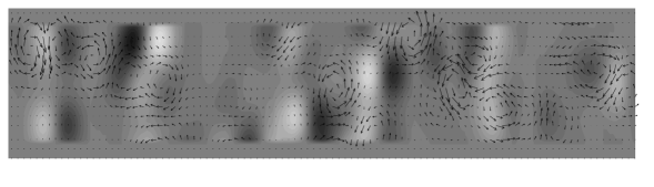
Figure 24: Cross-section of the velocity field for the 100-eddy turbulence model ${\cal B}$ in the $xy$-plane at an arbitrary time of the simulation. White colour denotes positive $u_{z}$, black colour negative $u_{z}$.

A single vortex rotates with the velocity $\omega$ around its axis of rotation and moves with the velocity up and down along this axis. The eddy itself has also its own lifetime growing linearly with subsequent time steps. The vortex velocity $\omega$ as well as the vertical drift $w$ decrease with the distance $r$ from the axis and with the lifetime $t$ according to

$$(\omega,w)=(\omega_{0},w_{0})\cdot e^{-0.5\bigg{(}\big{(}r/l_{\rm corr}\big{)}^{2}+\big{(}z/z_{\rm corr}\big{)}^{2}\bigg{)}}\cdot e^{-t/\tau_{\rm corr}},$$ (71)

where $l_{\rm corr}$ is the adopted vortex radius (Otmianowska-Mazur et al., 1992), $z_{\rm corr}$ is its length scale along the axis of rotation and $\tau_{\rm corr}$ is the eddy decay time scale. All velocities are truncated at $3l_{\rm corr}$ and $3z_{\rm corr}$. In the model all vortices are orientated like right-handed screws. The resulting motion has maximum helicity. A uniform distribution of eddies in a 3D space is approximated with 12 possible inclination angles of their rotational axes to the $xy$-plane.

The initial state is a number $N$ of moving turbulent cells having random inclinations and positions in the $xy$-plane. After an assumed period of time (one or more time steps), a fraction of them, $R_{\rm tur}$ (the ratio of the new-eddies number to $N$), is changed to new ones with different randomly given position, inclination and with lifetime starting from zero. The situation repeats itself continuously with time.

Table 2: Input and output for the turbulence models ${\cal A,B,C}$ and ${\cal D}$. $N$ is the eddy population of the equator, $R_{\rm tur}$ the eddy birth rate, other quantities and normalizations as explained in the text.

	$l_{\rm corr}$	$\tau_{\rm corr}$	$N$	$R_{\rm tur}$	$\eta_{\rm T}$	$\sigma(\eta_{\rm T})$	$\alpha_{xx}$	$\sigma(\alpha_{xx})$	$\alpha_{yy}$	$\sigma(\alpha_{yy})$
${\cal A}$	1	10	200	1.0	0.191	0.086	$-$0.046	0.048	$-$0.077	0.055
${\cal B}$	2	20	100	0.7	0.336	0.208	$-$0.029	0.063	$-$0.048	0.059
${\cal C}$	4	40	50	0.005	1.045	0.860	$-$0.029	0.119	$-$0.039	0.110
${\cal D}$	8	80	25	0.0003	1.793	2.278	$-$0.015	0.136	$-$0.017	0.110

The vortex radius $l_{\rm corr}$ as well as the decay time $\tau_{\rm corr}$ and the fraction of the new turbulent cells $R_{\rm tur}$ are varied for four cases given in Tables 2 and 3 in normalized units (cgs units for time, velocity and diffusivity result after multiplication with $2.5\cdot 10^{4}$ s, $10^{5}$ cm/s and $2.5\cdot 10^{14}$ cm²/s).

We made numerical experiments with the following values for the vortex radius $l_{\rm corr}$ and the length scale $z_{\rm corr}$ in the $z$-direction in normalized units: 1, 2, 4 and 8. For successive length scales we choose the time scales 10, 20, 40 and 80. The ratio of both scales is always $l_{\rm corr}/\tau_{\rm corr}\cong 0.1$. In order to obtain the expected mean turbulent velocity value of 0.1, the fraction of new vortices $R_{\rm tur}$ is also varied (Table 2; cf. Otmianowska-Mazur et al., 1997).

8.2 Numerical Experiments

The simulations deliver time series of the turbulence intensity, the eddy diffusivity and the $\alpha$-coefficients, and a standard deviation $\sigma$ from their temporal averages

$$\sigma=\sqrt{E[(X-E(X))^{2}]},$$ (72)

where $E(X)$ is the time average of a random variable $X$. The standard deviation measures the amplitude of the fluctuations compared with the temporal mean of a given quantity. Table 2 lists the input model parameters $l_{\rm corr}$, $\tau_{\rm corr}$, and $R_{\rm tur}$ and the coefficients obtained. The ratios of the standard deviations to their mean values,

$$S_{\eta}=\sigma(\eta)/\mid\eta\mid,$$ (73)

are given in Table 3.

Table 3: The ratio $S$ of fluctuations and mean values.

model	$S_{\eta_{\rm T}}$	$S_{\alpha_{xx}}$	$S_{\alpha_{yy}}$
${\cal A}$	0.45	1.03	0.72
${\cal B}$	0.62	2.13	1.24
${\cal C}$	0.82	4.10	2.79
${\cal D}$	1.27	8.94	6.62

Figure 25: Time series for turbulence intensity, eddy diffusivity and alpha-tensor components $\alpha_{xx}$ and $\alpha_{yy}$ for turbulence model $\cal A$. For time, velocity ($u$ and $\alpha$) and diffusivity cgs units result after multiplication with $2.5\cdot 10^{4}$ s, $10^{5}$ cm/s and $2.5\cdot 10^{14}$ cm²/s.

Figure 26: The same as in Fig. 25 but for model ${\cal D}$.

The results for a model ${\cal A}$ with $l_{\rm corr}=1$ and $\tau_{\rm corr}=10$, which is the sample of shortest lifetimes and smallest spatial dimensions of individual vortices in our simulation sequence is given in Fig. 25. All computed quantities are drawn as a time series, each in its own normalized units according to their definitions. The three EMF-coefficients as well as the turbulence intensity show fluctuations around their mean values in time. The diffusion coefficient $\eta_{\rm T}$ possesses positive values during most of the time. There are also short periods with a negative $\eta_{\rm T}$. The negative values are not significant because the resulting mean $\eta_{\rm T}$ is always positive yielding 0.191 (Table 2) in normalized units. The ratio $S_{\eta_{\rm T}}$ is 0.45 (Table 3). Indeed, the value 0.191 corresponds to $\eta_{\rm T}\simeq\ \tau_{\rm corr}\ u_{\rm T}^{2},$ which gives 0.1 for this case. In contrast to $\eta_{\rm T}$, the coefficients $\alpha_{xx}$ and $\alpha_{yy}$ possess negative values during the major part of the time; for short periods, however, positive values are also present. The negative $\alpha$ results from the assumed non-zero, right-handed helicity of the vortices and is in agreement with the expectations. Averaged in time $\alpha_{xx}$ for model ${\cal A}$ is $-4.6\cdot 10^{3}{\rm cm}/{\rm s}$. For $\alpha_{yy}$ we get $-7.7\cdot 10^{3}{\rm cm}/{\rm s}$ resulting in a dynamo number of $C_{\alpha}=10$. It can be seen that $\alpha_{xx}$ is always slightly smaller than $\alpha_{yy}$. This fact is connected with the assumed averaging only along the $y$-axis, which certainly influences the value of $\alpha_{xx}$. Model ${\cal A}$ yields the ratios $\sigma(\alpha_{xx})/\mid\alpha_{xx}\mid=1.03$ and $\sigma(\alpha_{yy})/\mid\alpha_{yy}\mid=0.72$.

The second experiment, $\cal B$, uses doubled correlation lengths and times, $l_{\rm corr}=2$, $\tau_{\rm corr}=20$ (see also Fig. 24). A fraction of 0.7 new vortices at every time step was applied. The resulting fluctuations of $\eta_{\rm T}$ and $\alpha$-coefficients are higher than in the case $\cal A$ (Table 2). The averaged value of $\eta_{\rm T}$ increases to 0.336, yielding $8.5\cdot 10^{13}~{}{\rm cm}^{2}/{\rm s}$. The ratios $S_{\alpha_{xx}}$ and $S_{\alpha_{yy}}$ increase up to $2.13$ and $1.24$, respectively (Table 3). It means that the fluctuations of $\alpha$ are higher for larger eddies with longer lifetimes – as it should.

The experiment ${\cal D}$ works with largest correlation times and longest lifetimes, $l_{\rm corr}=8$ and $\tau_{\rm corr}=80$. The birth rate $R_{\rm tur}$ is 0.0003 per time step – really low in comparison with the previous cases. Fig. 26 presents the time series of studied quantities. The resulting fluctuations of the alpha coefficients are extremely high. The mean value of $\eta_{\rm T}$ is 1.793 ($4.5\cdot 10^{14}~{}{\rm cm}^{2}/{\rm s}$). The ratio $S_{\eta_{\rm T}}=1.27$ indicates the significant growth of the fluctuations compared with the mean value. The obtained ratios are $S_{\alpha_{xx}}=8.94$ and $S_{\alpha_{yy}}=6.62$. The averaged in time values of $\alpha_{xx}$ and $\alpha_{yy}$ decrease again to $-0.015$ ($-1.5\cdot 10^{3}{\rm cm}^{2}/{\rm s}$) and $-0.017$ ($-1.7\cdot 10^{3}{\rm cm}^{2}/{\rm s}$).

Table 3 summarizes the main results of our simulations. The fluctuations in the time series become more and more dominant with the decreasing number of eddies together with the increasing vortex size. The extreme case is plotted in Fig. 26. For such models the fluctuations of both the eddy diffusivity as well as the $\alpha$-effect are much higher than the averages. Even short-lived changes of the sign of the quantities were found.

The $\alpha$-effect fluctuations exceed those of the eddy diffusivity in all our models. The latter proves to be more stable than the $\alpha$-effect against dilution of the turbulence. This is a confirmation, indeed, for those studies in which an $\alpha$-effect time series is exclusively used in dynamo computations.

8.3 A Plane-layer Dynamo

Quite a few publications deal with the influence of stochastic $\alpha$-fluctuations upon dynamo-generated magnetic fields for various models. Choudhuri (1992) discussed a simple plane-wave dynamo basically in the linear regime. The fluctuations adopted are as weak as about 10 %. While in the $\alpha\Omega$-regime the oscillations are hardly influenced, the opposite is true for the $\alpha^{2}$-dynamo. In the latter regime the solution suffers dramatic and chaotic changes even for rather weak disturbances. In the region between the both regimes the remaining irregular variations are suppressed in a model with nonlinear feedback formulated as a traditional $\alpha$-quenching.

A plane 1D $\alpha^{2}\Omega$-model similar to that of Section 6.1 is used to illustrate the influence of the fluctuating turbulence coefficients on a mean-field dynamo. It is not an overshoot dynamo (cf. Ossendrijver and Hoyng, 1996). The plane has infinite extent in the radial ($x$) and the azimuthal ($y$) direction, the boundaries are in the $z$-direction. Hence, we assume that the magnetic field components in both azimuthal direction, ($B$), and radial direction, ($\partial A/\partial z$), depend on $z$ only. Note that $z$ points opposite to the colatitude $\theta$.

The $\alpha$-tensor has only one component (given in Section 2.3) vanishing at the equator, and it is assumed here to vanish also at the poles. The magnetic feedback is considered to be conventional $\alpha$-quenching: $\alpha=\hat{\alpha}\alpha_{0}\Psi(B_{\rm tot})$ with $\Psi(B_{\rm tot})\propto B_{\rm tot}^{-2}$. The diffusivity is spatially uniform. The normalized dynamo equations are given in (62) and (63).

Figure 27: Dynamo-induced magnetic toroidal fields for the turbulence models $\cal O$ (27a), $\cal A$ (27b), $\cal B$ (27c) and ${\cal D}$ (27d). LEFT: time series, RIGHT: power spectra. The real time unit is 2.7 years.

Positive $C_{\alpha}$ describes a positive $\alpha$ in the northern hemisphere and a negative one in the southern hemisphere. $C_{\Omega}$ defines the amplitude of the differential rotation, positive $C_{\Omega}$ represents positive shear $\partial\Omega/\partial r$. The dynamo operates with a positive $\alpha$-effect in the northern hemisphere. Our dynamo numbers are $C_{\alpha}=5$ and $C_{\Omega}=200$. The turbulence models ${\cal A,B}$ and ${\cal D}$ are applied, flow patterns with small (${\cal A}$), medium (${\cal B}$) and with very large (${\cal D}$) eddies are used.

A magnetic dipole field oscillating with a (normalized) period of 1.46 (Fig. 27a) is induced by a dynamo model without EMF-fluctuations ($N\to\infty$, called ${\cal O}$). The period corresponds to an activity cycle of 8 years in physical units. Also the turbulence model ${\cal B}$ produces an oscillating dipole but with a much more complicated temporal behaviour (Fig. 27c). It is not a single oscillation, the power spectrum forms a rather broad line with substructures. The ‘quality’,

$$Q={\omega_{\rm cyc}\over\Delta\omega_{\rm cyc}},$$ (74)

of this line (with $\Delta\omega_{\rm cyc}$ as its half-width) proves to be about 2.9. This value close to the observed quality of the solar cycle is produced here by a turbulence model with about 100 eddies along the equator (see also Ossendrijver et al., 1996). There are also remarkable variations of the magnetic cycle amplitude.

The turbulence field $\cal D$ lead, not suprisingly, to a highly irregular temporal behaviour in the magnetic quantities. Its power spectrum peaks at several periods (Fig. 27d). The overall shape of the spectrum, however, does not longer suggest any oscillations. The power of the lower frequencies is strongly increased, the high-frequency power decreases as $\omega_{\rm cyc}^{-5/3}$ like a Kolmogoroff spectrum, indicating the existence of chaos.

Our experiments basically show how the dilution of turbulence is able to transform a single-mode oscillation (for very many cells) to an oscillation with low quality (for moderate eddy population) and finally to a temporal behaviour close to chaos (for very few cells). It is possible that the observed low quality (33) of the solar cycle indicates the finite number of the giant cells driving the large-scale solar dynamo. Implications for the temporal evolution of the solar rotation law should be another output of such a cell number statistics. The consequences for rotation will be an independent test of the presented theory leading to the same number of eddies contributing to the turbulent angular momentum transport. For only ‘occasional’ turbulence a nontrivial time series for both the turbulence EMF-coefficients and the magnetic field is an unavoidable consequence.

9 References

Abramenko, V.I., Wang, T. and V.B. Yurchishin, Analysis of electric current helicity in active regions on the basis of vector magnetograms. Solar Phys., 168, 75 (1996).

Baliunas, S.L. and A.H. Vaughan, Stellar activity cycles. Annual Review of Astronomy and Astrophysics, 23, 379 (1985).

Baliunas, S.L., E. Nesme-Ribes, D. Sokoloff and W.H. Soon, A dynamo interpretation of stellar activity cycles. Astrophys. J., 460, 848 (1996).

Bao, S. and H. Zhang, Patterns of current helicity for solar cycle 22. Astrophys. J., 496, L43 (1998).

Barnes, J.R., A.C. Cameron, D.J. James, C.A. Watson and J.-F. Donati, Starspot coverage and differential rotation on PZ Tel, in Proc. Stellar clusters and associations: Convection, rotation, and dynamos, Palermo (1999).

Beer, J., S.M. Tobias and N.O. Weiss, An active Sun throughout the Maunder minimum. Solar Phys., 181, 237 (1998).

Belvedere, G., G. Lanzafame and M.R.E. Proctor, The latitude belts of solar activity as a consequence of a boundary-layer dynamo. Nature, 350, 481 (1991).

Braginsky, S.I., Self excitation of a magnetic field during the motion of a highly conducting fluid. Sov. Phys. JETP, 20, 726 (1964).

Brandenburg, A., I. Tuominen and D. Moss, On the nonlinear stability of dynamo models. Geophys. Astrophys. Fluid Dynam., 49, 129 (1989).

Brandenburg, A., Å. Nordlund, P. Pulkkinen, R.F. Stein and I. Tuominen, 3-D simulation of turbulent cyclonic magneto-convection. Astron. Astrophys., 232, 277 (1990).

Brandenburg, A., Simulating the solar dynamo, in The cosmic dynamo (eds. F. Krause, K.-H. Rädler and G. Rüdiger), Kluwer, Dordrecht, 111 (1993).

Brandenburg, A., Solar dynamos: Computational background, in Lectures on solar and planetary dynamos (eds. M.R.E. Proctor and A.D. Gilbert), Cambridge University Press, 117 (1994a).

Brandenburg, A., Hydrodynamical simulations of the solar dynamo, in Advances in solar physics (eds. G. Belvedere and M. Rodono), Springer, Heidelberg, 73 (1994b).

Brandenburg, A., Large scale turbulent dynamos, in Stellar and planetary magnetoconvection (eds. J. Brestenský, S. Ševčik), Acta Astr. et Geophys. Univ. Comenianae, XIX, 235 (1997).

Brandenburg, A. and K.J. Donner, The dependence of the dynamo alpha on vorticity. Mon. Not. R. Astr. Soc., 288, L29 (1997).

Brandenburg, A., S.H. Saar and C.R. Turpin, Time evolution of the magnetic activity cycle period. Astrophys. J., 498, 51 (1998).

Brandenburg, A. and D. Schmitt, Simulations of an alpha-effect due to magnetic buoyancy. Astron. Astrophys., 338, L55 (1998).

Brandenburg, A., Dynamo-generated turbulence and outflows from accretion discs. Phil. Trans. R. Soc. Lond. A, 358, 759 (2000).

Caligari, P., F. Moreno-Insertis and M. Schüssler, Emerging flux tubes in the solar convection zone. I. Asymmetry, tilt and emergence latitude. Astrophys. J., 441, 886 (1995).

Choudhuri, A.R., The evolution of loop structures in flux rings within the solar convection zone. Solar Phys., 123, 217 (1989).

Choudhuri, A.R., On the possibility of an $\alpha^{2}\omega$-type dynamo in a thin layer inside the Sun. Astrophys. J., 355, 733 (1990).

Choudhuri, A.R., Stochastic fluctuations of the solar dynamo. Astron. Astrophys., 253, 277 (1992).

Choudhuri, A.R., M. Schüssler and M. Dikpati, The solar dynamo with meridional circulation. Astron. Astrophys., 303, L29 (1995).

Christensen-Dalsgaard, J. and J. Schou, Differential rotation in the solar interior, in Seismology of the Sun and Sun-like stars (eds. V. Domingo and E.J. Rolfe), ESA SP-286, 149 (1988).

DeLuca, E.E. and P.A. Gilman, The solar dynamo, in Solar interior and atmosphere (eds. A.N. Cox, W.C. Livingston and M.S. Matthews), Arizona University Press, Tucson, 275 (1991).

Dikpati, M. and P. Charbonneau, A Babcock-Leighton flux transport dynamo with solar-like differential rotation. Astrophys. J., 518, 508 (1999).

Donahue, R.A. and S.L. Baliunas, Evidence of differential surface rotation in the solar-type star HD 114710. Astrophys. J., 393, L63 (1992).

Donati, J.-F. and A.C. Cameron, Differential rotation and magnetic polarity patterns on AB Doradus. Mon. Not. R. Astr. Soc., 291, 1 (1997).

Durney, B.R. and R.D. Robinson, On an estimate of the dynamo-generated magnetic fields in late-type stars. Astrophys. J., 253, 290 (1982).

Durney, B.R., On the behavior of the angular velocity in the lower part of the solar convection zone. Astrophys. J., 338, 509 (1989).

Durney, B.R., On a Babcock-Leighton dynamo model with a deep-seated generating layer for the toroidal magnetic field. Solar Phys., 160, 213 (1995).

Durney, B.R., On a Babcock-Leighton dynamo model with a deep-seated generating layer for the toroidal magnetic field, II. Solar Phys., 166, 231 (1996).

Dziembowski, W.A. and P.R. Goode, Seismology for the fine structure in the Sun’s oscillations varying with its activity cycle. Astrophys. J., 376, 782 (1991).

Fan, Y., G.H. Fisher and E.E. DeLuca, The origin of morphological asymmetries in bipolar active regions. Astrophys. J., 405, 390 (1993).

Ferrière, K., The full alpha-tensor due to supernova explosions and superbubbles in the galactic disk. Astrophys. J., 404, 162 (1993).

Ferriz-Mas, A. and M. Schüssler, Instabilities of magnetic flux tubes in a stellar convection zone. I. Equatorial flux rings in differentially rotating stars. Geophys. Astrophys. Fluid Dynam., 72, 209 (1993).

Ferriz-Mas, A., D. Schmitt and M. Schüssler, A dynamo effect due to instability of magnetic flux tubes. Astron. Astrophys., 289, 949 (1994).

Ferriz-Mas, A. and M. Schüssler, Instabilities of magnetic flux tubes in a stellar convection zone. II. Flux rings outside the equatorial plane. Geophys. Astrophys. Fluid Dynam., 81, 233 (1995).

Frick, P., D. Galyagin, D.V. Hoyt, E. Nesme-Ribes, K.H. Schatten, D. Sokoloff and V. Zakharov, Wavelet analysis of solar activity recorded by sunspot groups. Astron. Astrophys., 328, 670 (1997a).

Frick, P., E. Nesme-Ribes and D. Sokoloff, Wavelet analysis of solar activity recorded by sunspot groups and solar diameter data, in Stellar and planetary magnetoconvection (eds. J. Brestenský and S. Ševčik), Acta Astron. et Geophys. Univ. Comenianae, XIX, 113 (1997b).

Gilman, P.A., What can we learn about solar cycle mechanisms from observed velocity fields, in The solar cycle (ed. K.L. Harvey), ASP Conf. Ser., 27, 241 (1992).

Glatzmaier, G.A. and R. Roberts, A three-dimensional convective dynamo solution with rotating and finitely conducting inner core and mantle. Phys. Earth Planet. Inter., 91, 63 (1995).

Hale, G.E., The fields of force in the atmosphere of the Sun. Nature, 119, 708 (1927).

Hempelmann, A., J. Schmitt and K. Stȩpieǹ, Coronal X-ray emission of cool stars in relation to chromospheric activity and magnetic cycles. Astron. Astrophys., 305, 284 (1996).

Hood, L.L. and J.L. Jirikowic, A probable approx. 2400 year solar quasi-cycle in atmospheric delta C-14, in Climate impact of solar variability, NASA, 98 (1990).

Howard, R.F. and B.J. LaBonte, The sun is observed to be a torsional oscillator with a period of 11 years. Astrophys. J., 239, L33 (1980).

Hoyng, P., Turbulent transport of magnetic fields. III. Stochastic excitation of global magnetic modes. Astrophys. J., 332, 857 (1988).

Hoyng, P., Helicity fluctuations in mean field theory: an explanation for the variability of the solar cycle. Astron. Astrophys., 272, 321 (1993).

Hoyng, P., D. Schmitt and L.J.W. Teuben, The effect of random alpha-fluctuations and the global properties of the solar magnetic field. Astron. Astrophys., 289, 265 (1994).

Jennings, R.L. and N.O. Weiss, Symmetry breaking in stellar dynamos. Mon. Not. R. Astr. Soc., 252, 249 (1991).

Kaisig, M., G. Rüdiger and H.W. Yorke, The alpha-effect due to supernova explosions. Astron. Astrophys., 274, 757 (1993).

Keinigs, R.K., A new interpretation of the alpha effect. Phys. Fluids, 76, 2558 (1983).

Kitchatinov, L.L., Turbulent transport of angular momentum and differential rotation. Geophys. Astrophys. Fluid Dynam., 35, 93 (1986).

Kitchatinov, L.L. and G. Rüdiger, Magnetic-field advection in inhomogeneous turbulence. Astron. Astrophys., 260, 494 (1992).

Kitchatinov, L.L., Turbulent transport of magnetic fields and the solar dynamo, in The cosmic dynamo (eds. F. Krause, K.-H. Rädler and G. Rüdiger), Kluwer, Dordrecht, 13 (1993).

Kitchatinov, L.L. and V.V. Pipin, Mean-field buoyancy. Astron. Astrophys., 274, 647 (1993).

Kitchatinov, L.L. and G. Rüdiger, Lambda-effect and differential rotation in stellar convection zones. Astron. Astrophys., 276, 96 (1993).

Kitchatinov, L.L., G. Rüdiger and M. Küker, $\Lambda$-quenching as the nonlinearity in stellar-turbulence dynamos. Astron. Astrophys., 292, 125 (1994a).

Kitchatinov, L.L., V.V. Pipin and G. Rüdiger, Turbulent viscosity, magnetic diffusivity, and heat conductivity under the influence of rotation and magnetic field. Astron. Nachr., 315, 157 (1994b).

Kitchatinov, L.L. and G. Rüdiger, Differential rotation in solar-type stars: revisiting the Taylor number puzzle. Astron. Astrophys., 299, 446 (1995).

Kitchatinov, L.L. and G. Rüdiger, Differential rotation models for late-type dwarfs and giants. Astron. Astrophys., 344, 911 (1999).

Knobloch, E. and A.S. Landsberg, A new model of the solar cycle. Mon. Not. R. Astr. Soc., 278, 294 (1996).

Knobloch, E., S.M. Tobias and N.O. Weiss, Modulation and symmetry changes in stellar dynamos. Mon. Not. R. Astr. Soc., 297, 1123 (1998).

Köhler, H., The solar dynamo and estimates of the magnetic diffusivity and the $\alpha$-effect. Astron. Astrophys., 25, 467 (1973).

Kosovichev, A.G., J. Schou, P.H. Scherrer, et al., Structure and rotation of the solar interior: Initial results from the MDI medium-l program. Solar Phys., 170, 43 (1997).

Krause, F., Eine Lösung des Dynamoproblems auf der Grundlage einer linearen Theorie der magnetohydrodynamischen Turbulenz. Thesis, Universität Jena (1967).

Krause, F. and K.-H. Rädler, Mean-field magnetohydrodynamics and dynamo theory, Pergamon Press, Oxford (1980).

Krause, F. and R. Meinel, Stability of simple nonlinear $\alpha^{2}$-dynamos. Geophys. Astrophys. Fluid Dynam., 43, 95 (1988).

Krause, F. and H.-J. Schmidt, A low-dimensional attractor for modeling the reversals of the Earth’s magnetic field. Phys. Earth Planet. Inter., 52, 23 (1988).

Krivodubskij, V.N. and M. Schultz, Complete alpha-tensor for solar dynamo, in The cosmic dynamo (eds. F. Krause, K.-H. Rädler and G. Rüdiger), Kluwer, Dordrecht, 25 (1993).

Küker, M., G. Rüdiger and L.L. Kitchatinov, An alpha-omega model of the solar differential rotation. Astron. Astrophys., 279, 1 (1993).

Küker, M., G. Rüdiger and V.V. Pipin, Solar torsional oscillations as due to the magnetic quenching of the Reynolds stress. Astron. Astrophys., 312, 615 (1996).

Küker, M., R. Arlt and G. Rüdiger, The Maunder minimum as due to magnetic $\Lambda$-quenching. Astron. Astrophys., 343, 977 (1999).

Kurths, J., A. Brandenburg, U. Feudel and W. Jansen, Chaos in nonlinear dynamo models, in The cosmic dynamo (eds. F. Krause, K.-H. Rädler and G. Rüdiger), Kluwer, Dordrecht, 83 (1993).

Kurths, J., U. Feudel, W. Jansen, U. Schwarz and H. Vos, Solar variability: simple models and proxy data, in Proc. Int. School Physics Enrico Fermi, Course CXXXIII (eds. G. Castagnoli and A. Provenzale), IOS Press, Amsterdam, 247 (1997).

Levy, E.H., Physical assessment of stellar dynamo theory, in Cool stars, stellar systems, and the Sun (eds. M.S. Giampapa and J.A. Bookbinder), ASP Conf. Ser., 26, 223 (1992).

Low, B.C., Solar activity and the corona. Solar Phys., 167, 217 (1996).

Malkus, W.V.R. and M.R.E. Proctor, The macrodynamics of $\alpha$-effect dynamos in rotating fluids. J. Fluid Mech., 67, 417 (1975).

Markiel, J.A., Thomas, J.H., Solar interface dynamo models with a realistic rotation profile. Astrophys. J., 523, 827 (1999).

Moffatt, K.H., Magnetic field generation in electrically conducting fluids, Cambridge University Press (1978).

Moreno-Insertis, F., Rise times of horizontal magnetic flux tubes in the convection zone of the sun. Astron. Astrophys., 122, 241 (1983).

Moss, D., I. Tuominen and A. Brandenburg, Nonlinear dynamos with magnetic buoyancy in spherical geometry. Astron. Astrophys., 228, 284 (1990).

Moss, D., A. Brandenburg, R. Tavakol and I. Tuominen, Stochastic effects in mean field dynamos. Astron. Astrophys., 265, 843 (1992).

Nesme-Ribes, E., D. Sokoloff, J.C. Ribes and M. Kremliovsky, The maunder minimum and the solar dynamo, in The solar engine and its influence on terrestrial atmosphere and climate (ed. E. Nesme-Ribes), Springer-Verlag, Berlin, 71 (1994).

Noyes, R.W., N.O. Weiss and A.H. Vaughan, The relation between stellar rotation rate and activity cycle periods. Astrophys. J., 287, 769 (1984).

Ossendrijver, A.J.H. and P. Hoyng, Stochastic and nonlinear fluctuations in a mean field dynamo. Astron. Astrophys., 313, 959 (1996).

Ossendrijver, A.J.H., P. Hoyng and D. Schmitt, Stochastic excitation and memory of the solar dynamo. Astron. Astrophys., 313, 938 (1996).

Ossendrijver, A.J.H., On the cycle periods of stellar dynamos. Astron. Astrophys., 323, 151 (1997).

Otmianowska-Mazur, K., M. Urbanik and A. Terech, Magnetic field in a turbulent galactic disk. Geophys. Astrophys. Fluid Dynam., 66, 209 (1992).

Otmianowska-Mazur, K., G. Rüdiger, D. Elstner and R. Arlt, The turbulent EMF as a time series and the ‘quality’ of dynamo cycles. Geophys. Astrophys. Fluid Dynam., 86, 229 (1997).

Parker, E.N., The generation of magnetic fields in astrophysical bodies. X - Magnetic buoyancy and the solar dynamo. Astrophys. J., 198, 205 (1975).

Parker, E.N., The dynamo dilemma. Solar Phys., 110, 11 (1987).

Pevtsov, A.A., Canfield, R.C. and T.R. Metcalf, Latitudinal variation of helicity of photospheric magnetic fields. Astrophys. J., 440, L109 (1995).

Pipin, V.V., The Gleissberg cycle by a nonlinear $\alpha\Lambda$ dynamo. Astron. Astrophys., 346, 295 (1999).

Prautzsch, T., The dynamo mechanism in the deep convection zone of the Sun, in Theory of solar and planetary dynamos (eds. P.C. Matthews and A.M. Rucklidge), Cambridge University Press, 249 (1993).

Rädler, K.-H., Zur Elektrodynamik turbulent bewegter leitender Medien. Teil II. Zeitschr. f. Naturforschg., 23a, 1851 (1968).

Rädler, K.-H. and N. Seehafer, Relations between helicities in mean-field dynamo models, in Topological Fluid Mechanics (eds. H.K. Moffatt and A. Tsinober) Cambridge University Press, 157 (1990).

Ribes, J.C. and E. Nesme-Ribes, The solar sunspot cycle in the Maunder minimum AD1645. Astron. Astrophys., 276, 549 (1993).

Roberts, P.H., Kinematic dynamo models. Phil. Trans. R. Soc. Lond. A., 272, 663 (1972).

Roberts, P.H. and M. Stix, $\alpha$-Effect dynamos by the Bullard-Gellman formalism. Astron. Astrophys., 18, 453 (1972).

Rozelot, J.P., On the chaotic behaviour of the solar activity. Astron. Astrophys., 297, L45 (1995).

Rüdiger, G., I. Tuominen, F. Krause and H. Virtanen, Dynamo-generated flows in the Sun. Astron. Astrophys., 166, 306 (1986).

Rüdiger, G., Differential rotation and stellar convection: Sun and solar-type stars, Gordon and Breach Science Publishers, New York (1989).

Rüdiger, G. and L.L. Kitchatinov, $\alpha$-effect and $\alpha$-quenching. Astron. Astrophys., 269, 581 (1993).

Rüdiger, G., L.L. Kitchatinov, M. Küker and M. Schultz, Dynamo models with magnetic diffusivity-quenching. Geophys. Astrophys. Fluid Dynam., 78, 247 (1994).

Rüdiger, G. and A. Brandenburg, A solar dynamo in the overshoot layer: cycle period and butterfly diagram. Astron. Astrophys., 296, 557 (1995).

Rüdiger, G. and R. Arlt, Cycle times and magnetic amplitudes in nonlinear 1D $\alpha^{2}\Omega$-dynamos. Astron. Astrophys., 316, L17 (1996).

Rüdiger, G. and L.L. Kitchatinov, The slender solar tachocline: a magnetic model. Astron. Nachr., 318, 273 (1997).

Rüdiger, G. and M. Schultz, Nonlinear galactic dynamo models with magnetic-supported interstellar gas-density stratification. Astron. Astrophys., 319, 781 (1997).

Rüdiger, G. and V.V. Pipin, Astron. Astrophys. in prep. (2000).

Saar, S.H. and S.L. Baliunas, Recent advances in stellar cycle research, in The solar cycle (ed. K.L. Harvey), ASP Conf. Ser., 27, 150 (1992a).

Saar, S.H. and S.L. Baliunas, The magnetic cycle of $\kappa$ Ceti (G5V), in The solar cycle (ed. K.L. Harvey), ASP Conf. Ser., 27, 197 (1992b).

Saar, S.H., Recent measurements of stellar magnetic fields, in Stellar surface structure (eds. K.G. Strassmeier and J.L. Linsky), Kluwer, Dordrecht, 237 (1996).

Saar, S.H. and A. Brandenburg, Time evolution of the magnetic activity cycle period. II. Results for an expanded stellar sample. Astrophys. J., 524, 295 (1999).

Schlichenmaier, R. and M. Stix, The phase of the radial mean field in the solar dynamo. Astron. Astrophys., 302, 264 (1995).

Schmitt, D., Thesis, Universität Göttingen (1985).

Schmitt, D., An $\alpha\omega$-dynamo with an $\alpha$-effect due to magnetostrophic waves. Astron. Astrophys., 174, 281 (1987).

Schmitt, D. and M. Schüssler, Non-linear dynamos. I. One-dimensional model of a thin layer dynamo. Astron. Astrophys., 223, 343 (1989).

Schmitt, D., The solar dynamo, in The cosmic dynamo (eds. F. Krause, K.-H. Rädler and G. Rüdiger), Kluwer, Dordrecht, 1 (1993).

Schmitt, D., M. Schüssler and A. Ferriz-Mas, Intermittent solar activity by an on-off dynamo. Astron. Astrophys., 311, L1 (1996).

Schüssler, M., The solar torsional oscillation and dynamo models of the solar cycle. Astron. Astrophys., 94, 17 (1981).

Schüssler, M., Magnetic fields and the rotation of the solar convection zone, in The internal solar angular velocity (ed. R. Durney), Reidel, Dordrecht, 303 (1987).

Schwarz, U., Zeitreihenanalyse astrophysikalischer Aktivitätsphänomene. Thesis, Universität Potsdam (1994).

Seehafer, N., Electric current helicity in the solar atmosphere. Solar Phys., 125, 219 (1990).

Soon, W.H., S.L. Baliunas and Q. Zhang, An interpretation of cycle periods of stellar chromospheric activity. Astrophys. J., 414, L33 (1993).

Spiegel, E.A. and N.O. Weiss, Magnetic activity and variations in solar luminosity. Nature, 287, 616 (1980).

Spörer, G., Über die Periodizität der Sonnenflecken seit dem Jahre 1618. Vierteljahresschrift der Astron. Ges., 22, 323 (1887).

Steenbeck, M. and F. Krause, Zur Dynamotheorie stellarer und planetarer Magnetfelder. I. Berechnung sonnenähnlicher Wechselfeldgeneratoren. Astron. Nachr., 291, 49 (1969).

Stix, M., Differential rotation and the solar dynamo. Astron. Astrophys., 47, 243 (1976).

Stix, M. and D. Skaley, The equation of state and the frequencies of solar p modes. Astron. Astrophys., 232, 234 (1990).

Stix, M., The solar dynamo. Geophys. Astrophys. Fluid Dynam., 62, 211 (1991).

Tobias, S.M., Grand minima in nonlinear dynamos. Astron. Astrophys., 307, L21 (1996).

Tobias, S.M., The solar cycle: parity interactions and amplitude modulation. Astron. Astrophys., 322, 1007 (1997).

Tobias, S.M., Relating stellar cycle periods to dynamo calculations. Mon. Not. R. Astr. Soc., 296, 653 (1998).

Tuominen, I., G. Rüdiger and A. Brandenburg, Observational constraints for solar-type dynamos, in Activity in cool star envelopes (eds. Havnes et al.), Kluwer, Dordrecht, 13 (1988).

Vainshtein, S.I. and F. Cattaneo, Nonlinear restriction on dynamo action. Astrophys. J., 393, 165 (1992).

van Ballegooijen, A.A., The overshoot layer at the base of the solar convective zone and the problem of magnetic flux storage. Astron. Astrophys., 113, 99 (1982).

van Ballegooijen, A.A., Understanding the solar cycle, in Synoptic solar physics (eds. K.S. Balasubramaniam, J. Harvey and D. Rabin), ASP Conf. Ser., 140, 17 (1998).

Verma, V.K., On the north-south asymmetry of solar activity cycles. Astrophys. J., 403, 797 (1993).

Vishniac, E.T. and A. Brandenburg, An incoherent $\alpha\omega$-dynamo in accretion disks. Astrophys. J., 475, 263 (1997).

Vos, H., J. Kurths and U. Schwarz, Reconstruction of grand minima of solar activity from radiocarbon data – linear and nonlinear signal analysis. J. Geophys. Res. A, 101, 15637 (1996).

Vos, H., A. Sanchez, B. Zolitschka, A. Brauer and J.F.W. Negendank, Solar activity variations recorded in varved sediments from the crater lake of Holzmaar – A maar lake in the Westeifel volcanic field, Germany. Surv. Geophys., 18, 163 (1997).

Wälder, M., W. Deinzer and M. Stix, Dynamo action associated with random waves in a rotating stratified fluid. J. Fluid Mech., 96, 207 (1980).

Weiss, N.O., F. Cattaneo and C.A. Jones, Periodic and aperiodic dynamo waves. Geophys. Astrophys. Fluid Dynam., 30, 305 (1984).

Weiss, N.O., Solar and stellar dynamos, in Lectures on solar and planetary dynamos (eds. M.R.E. Proctor and A.D. Gilbert), Cambridge University Press, 59 (1994).

Wittmann, A., The sunspot cycle before the maunder minimum. Astron. Astrophys., 66, 93 (1978).

Yoshimura, H., Phase relation between the poloidal and toroidal solar-cycle general magnetic fields and location of the origin of the surface magnetic fields. Solar Phys., 50, 3 (1976).

Yoshimura, H., Solar cycle Lorentz force waves and the torsional oscillations of the sun. Astrophys. J., 247, 1102 (1981).

Ziegler, U., H.W. Yorke and M. Kaisig, The role of supernovae for the galactic dynamo: The full alpha-tensor. Astron. Astrophys., 305, 114 (1996).