In Hot Pursuit of the Hidden Companion of $\eta$ Carinae: An X-ray Determination of the Wind Parameters

We present X-ray spectral fits to a recently obtained Chandra grating spectrum of $\eta$ Carinae, one of the most massive and powerful stars in the Galaxy and which is strongly suspected to be a colliding wind binary system. Hydrodynamic models of colliding winds are used to generate synthetic X-ray spectra for a range of mass-loss rates and wind velocities. They are then fitted against newly acquired Chandra grating data. We find that due to the low velocity of the primary wind ($\approx 500\hbox{${\rm{\rm\thinspace km}{\rm\thinspace s}^{-1}\,}$}$), most of the observed X-ray emission appears to arise from the shocked wind of the companion star. We use the duration of the lightcurve minimum to fix the wind momentum ratio at $\eta=0.2$. We are then able to obtain a good fit to the data by varying the mass-loss rate of the companion and the terminal velocity of its wind. We find that $\hbox{${\dot{M}}$}\,_{2}\approx 10^{-5}\;\hbox{${\rm\hbox{${\rm\thinspace M_{\odot}}$}{\rm\thinspace yr}^{-1}\,}$}$ and $v_{\infty_{2}}\approx 3000\;\hbox{${\rm{\rm\thinspace km}{\rm\thinspace s}^{-1}\,}$}$. With observationally determined values of $\approx 500-700\;\hbox{${\rm{\rm\thinspace km}{\rm\thinspace s}^{-1}\,}$}$ for the velocity of the primary wind, our fit implies a primary mass-loss rate of $\hbox{${\dot{M}}$}\,_{1}\approx 2.5\times 10^{-4}\;\hbox{${\rm\hbox{${\rm\thinspace M_{\odot}}$}{\rm\thinspace yr}^{-1}\,}$}$. This value is smaller than commonly inferred, although we note that a lower mass-loss rate can reduce some of the problems noted by Hillier et al. (HDIG2001 (2001)) when a value as high as $10^{-3}\;\hbox{${\rm\hbox{${\rm\thinspace M_{\odot}}$}{\rm\thinspace yr}^{-1}\,}$}$ is used. The wind parameters of the companion are indicative of a massive star which may or may not be evolved. The line strengths appear to show slightly sub-solar abundances, although this needs further confirmation. Based on the over-estimation of the X-ray line strengths in our model, and re-interpretation of the HST/FOS results, it appears that the homunculus nebula was produced by the primary star.

1 Introduction

The superluminous star $\eta$ Carinae (HD 93308, HR 4210) continues to be extensively studied over a host of different wavelengths, yet remains intriguingly enigmatic. It is amongst the most unstable stars known. In the 1840s, and again in the 1890s, it underwent a series of giant outbursts (e.g. Viotti V1995 (1995)) which ejected large masses of material into the surrounding medium. HST images of the resulting bipolar nebula (e.g. Morse et al. MDB1998 (1998)), known as the Homunculus, show it to be amongst the most spectacular in our Galaxy. The central object is now largely obscured by dust, and the cause of the outbursts and the nature of the underlying star (at outburst and today) remain speculative. The source continues to show brightness fluctuations and emission-line variations. Further details of $\eta$ Car can be found in the review by Davidson & Humphreys (DH1997 (1997)).

In recent years evidence for binarity in this system has been accumulating. Damineli (D1996 (1996)) first noted a 5.5 yr period in the variability of the He I 10830 ${\rm\AA}$ line. Further photometric and radial velocity studies (Damineli et al. DCL1997 (1997), D2000 (2000)), X-ray observations (Tsuboi et al. TKSP1997 (1997); Corcoran et al. CFPSD2000 (2000) and references therein), and radio data (Duncan et al. D1995 (1995), DWRL1999 (1999)) have supported the 5.5 yr period and the binary hypothesis. However, the ground based radial velocity curve was not confirmed by higher resolution spectra with STIS, indicating that at least the time of periastron passage is not well defined by the UV and optical spectra (Corcoran et al. 2001a ). A comparison of the abundances from the central object(s) and the composition of the Homunculus nebula has also determined that there are at least two stars in this system (Lamers et al. LLPW1998 (1998)).

$\eta$ Car is often classified as a luminous blue variable (LBV). These are massive stars believed to be in a rapid and unstable evolutionary phase in which many solar masses of material are ejected into the interstellar medium over a relatively short period of time ($\approx 10^{4}$ yr). LBVs are regarded as a key phase in the evolution of massive stars, during which a transition into a Wolf-Rayet star occurs (e.g. Langer et al. L1994 (1994); Maeder & Meynet MM2001 (2001)). Due to their rarity and complex nature however, we unfortunately still have no definitive theory for mass-loss during the LBV stage. The majority of proposed mechanisms to drive LBV instabilities, the onset of higher mass-loss rates and underlying eruptions, are concerned with the importance of radiation pressure within the outer envelope of the LBV, and for example utilize pulsational instabilities (e.g. Guzik et al. GCD1999 (1999)), dynamical instabilities (e.g. Stothers & Chin SC1993 (1993)), or presuppose Eddington-like instabilities. The latter could arise from an enhancement in opacity as the star moves to lower temperatures (e.g. Lamers Lam1997 (1997)), or from the influence of rotation (e.g. Langer Lan1997 (1997); Zethson et al. Z1999 (1999)). Alternatively, the possibility that binarity plays a fundamental role in explaining observed LBV outburst properties has also been considered (Gallagher G1989 (1989)), though most LBVs are not known binaries. Clearly, determining the wind and stellar properties of LBV stars is paramount (see, for example, the discussions in Leitherer et al. L1994 (1994) and Nota et al. N1996 (1996)).

An important question is the degree to which binarity influences the properties of LBVs (i.e. do LBVs in binaries evolve differently than single LBVs?). So while the presence of a companion can be exploited to help measure the mass of such stars, we must bear in mind that binary LBVs and single LBVs may be quite distinct objects. Therefore, in order to use $\eta$ Car to understand some of the defining LBV characteristics such as their extremely high mass-loss rates, we first need to determine beyond all doubt that $\eta$ Car is in fact a binary, and then to determine the influence of the companion on the system.

Investigations over the last few years have already helped to form a basic picture of $\eta$ Car. The orbital parameters, although uncertain, indicate the presence of an early-type companion star, which will also have a powerful stellar wind. In such binaries, a region of hot shocked gas with temperatures in excess of 10 million K is created where the stellar winds collide (Prilutskii & Usov PU1976 (1976); Cherepashchuk C1976 (1976)). The wind-wind collision (WWC) region is expected to contribute to the observed emission from this system, particularly at X-ray and radio wavelengths. Previous X-ray observations revealed extended soft emission from the nebula and strong, hard, highly absorbed, and variable emission closest to the star (Corcoran et al. C1995 (1995); Weis et al. WDB2001 (2001)), in contrast to the emission characteristics from single stars, which are typically softer, much less absorbed, substantially weaker and relatively constant in intensity. Since 1996 Feb $\eta$ Car has been continuously monitored by RXTE in the 2–10 keV band (e.g. Corcoran et al. 2001a ). The lightcurve (Fig. 1) contains remarkable detail showing a slow, almost linear, rise to maximum over a period of $\approx 1$ yr, followed by a rapid drop to approximately 1/6 of the peak intensity for $\approx 3$ months, an almost as sharp rise to approximately 1/2 of the peak intensity level, and then almost constant intensity for $\approx 3/4$ of the proposed 5.5 yr orbital period. The drop to minimum was successfully predicted from numerical models of the WWC (Pittard et al. PSCI1998 (1998)) before being actually observed.

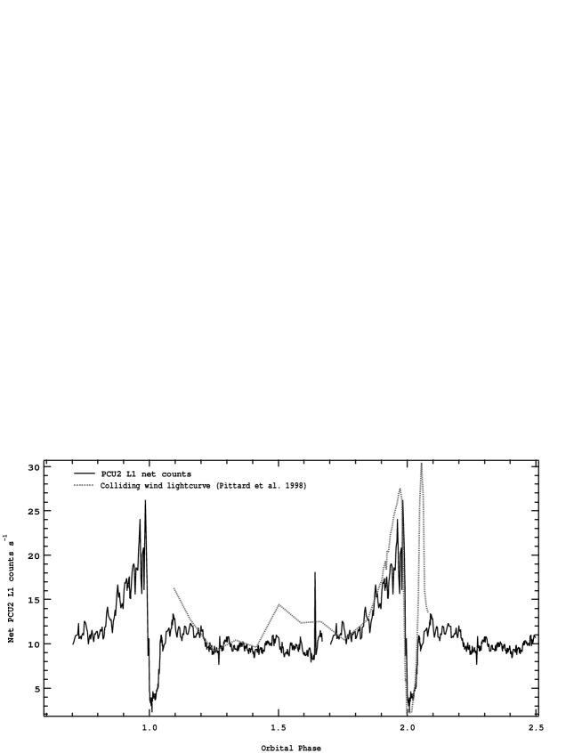
Figure 1: Lightcurve of $\eta$ Car observed with the RXTE satellite and phased to the 5.5 yr orbital period. Plotted are counts detected in layer 1 of the second proportional counter unit (PCU2) and a predicted lightcurve (Pittard et al. PSCI1998 (1998)) from a numerical model of the wind-wind collision. The two agree well, particularly the duration of the minimum. The rise from minimum is not in good agreement, but this is thought to be due to the limitations of modelling the wind collision in 2D. The rapid change in position angle of the stars through periastron passage skews the shock cone which causes the line of sight in fully 3D models to remain in the denser wind of the primary until later phases, increasing the absorption at these times (Pittard P2000 (2000))

.

Small scale quasi-periodic outbursts in the X-ray lightcurve have also been detected (Corcoran et al. CISDPS1997 (1997)). Estimates of changes in the timescale between successive flares as a function of phase were made by Davidson et al. (DIC1998 (1998)) for a variety of assumed orbital elements. RXTE X-ray observations obtained after the X-ray minimum seem to show a lengthening of the flare timescale (Ishibashi et al. I1999 (1999)), which indirectly support the binary model. The latest published X-ray observation of $\eta$ Car is of a high resolution grating spectrum taken with the Chandra X-ray observatory (Corcoran et al. 2001b ). Preliminary analysis has revealed the presence of strong forbidden line emission, which suggests that the density of the hot gas, $n_{\rm e}<10^{14}{\rm\thinspace cm}^{-3}$. This can be contrasted with the newly published X-ray grating spectra of the single stars $\theta^{1}$ Ori C (Schulz et al. SCHL2000 (2000)), $\zeta$ Ori (Waldron & Cassinelli WC2001 (2001)), and $\zeta$ Pup (Kahn et al. K2001 (2001)), all of which have weak forbidden lines (indicative of either high densities or high UV flux near the line forming region). This lends further support to a wind-wind collision model, although it is possible that some of the forbidden emission may be related to the surrounding nebula.

If $\eta$ Car is in fact a binary system, the orbital elements and stellar parameters are not yet tightly constrained by current observations. Ground-based observations (for which good phase coverage exist) are hampered by poor spatial resolution and thus suffer contamination from strong nebular emission. High-spatial resolution spectra have been obtained by STIS but phase coverage is currently very limited. HST STIS observations at two different phases of the 5.52 year cycle (Davidson et al. DI2000 (2000)) did not confirm the predicted variations in the radial velocity of the emission lines based on the ground-based radial velocity curve (Damineli et al. D2000 (2000)). If $\eta$ Car is a binary, it is vitally important to determine the stellar parameters of the companion so that the effect of the companion on observations can be understood and the correct stellar parameters of the primary can be derived.

1.1 X-ray Emission from Colliding Winds

The wealth of information contained in X-ray spectra of colliding wind binaries (e.g. the density, temperature, velocity, abundance, and distribution of the shocked gas in the wind collision region) has been a strong motivating force for observers and theorists alike in this field. Since the hot plasma in most colliding wind shocks is optically thin and collisionally ionized, and is generally assumed to be in collisional equilibrium, Raymond-Smith (Raymond & Smith RS1977 (1977)) or MEKAL (Mewe et al. MKL1995 (1995)) spectral models are normally fitted to such data (e.g. Zhekov & Skinner ZS2000 (2000); Rauw et al. RSPC2000 (2000); Corcoran et al. 2001b ). However, the multi-temperature, multi-density nature of the WWC region means that at best simple fits with one- or two-temperature Raymond-Smith models can only characterize the broad properties of the emission. In this way one can estimate an ‘average’ temperature of the shocked gas, and an ‘average’ absorbing column, but little is learned of the underlying stellar wind parameters. At worst the application of one- or two-temperature models to what is inherently multi-temperature emission can lead to spurious values of some of the fit parameters, e.g. abundances (cf. Strickland & Stevens SS1998 (1998)).

Complex numerical hydrodynamical models have often been applied to gain insight into colliding wind systems (e.g. Stevens et al. SBP1992 (1992), Pittard et al. PSCI1998 (1998)). However, while undoubtedly useful, their interpretation can be difficult, and to date there have been only two published papers where observed spectra are directly fitted with synthetic spectra from such models. In the pioneering work of Stevens et al. (S1996 (1996)), medium resolution ASCA spectra of the Wolf-Rayet binary $\gamma^{2}$ Velorum were fitted against a grid of synthetic spectra. In this fashion they were able to obtain direct estimates of the mass-loss rates and terminal velocities of the individual stellar winds. As mass-loss rates obtained from measures of radio flux or spectral line fits depend on a variety of untested assumptions, the importance of a new independent method to complement estimates from free-free radio or sub-mm observations, or from H$\alpha$ or UV spectral line fitting, cannot be stressed enough. Rates derived by Stevens et al. (S1996 (1996)) with this new method were significantly lower than the commonly accepted estimates for $\gamma^{2}$ Velorum based on radio observations, but an indication of the future benefits of this method was realized when both sets of estimates were later brought into agreement following a surprisingly large reduction in the distance to this star from Hipparcos data. We note that this method can also provide insights into the values of parameters which are otherwise virtually impossible to estimate, such as the mass-loss rate of the companion, $\hbox{${\dot{M}}$}\,_{2}$, or the characteristic ratio of the pre-shock electron and ion temperature (Zhekov & Skinner ZS2000 (2000)). The quality of recently available X-ray grating spectra now gives us access to important X-ray emission line diagnostics which should severely constrain models of the X-ray emission distribution. This means that stellar wind parameters can in principle be reliably estimated from analysis of X-ray grating spectra of colliding wind binaries.

In addition to testing the binary hypothesis, the Chandra grating spectrum of $\eta$ Car (Corcoran et al. 2001b ) provides the ideal opportunity to test the method developed by Stevens et al. (S1996 (1996)) against a spectrum of much higher spectral resolution, and to pin down important physical parameters of the system. In this paper we therefore fit the X-ray grating spectrum using a grid of colliding wind emission models to i) test the binary hypothesis, and ii) to attempt to obtain accurate estimates of the wind parameters of each star. The fact that we are able to obtain good fits, with sensible model parameters, gives us further confidence in the binary hypothesis. We also find that unlike the UV and optical work where fits to the primary are made difficult by significant contamination from the companion star, instead the X-ray emission arises from the shocked wind of the companion and suffers essentially zero contamination from the wind of the primary. Therefore the X-ray data uniquely samples parameters of the companion, in contrast to the optical analysis which probes the nature of the primary. In this sense our analysis is entirely complementary to the complex fits to the UV and optical HST spectrum of $\eta$ Car by Hillier et al. (HDIG2001 (2001)). Our analysis also provides us with a new estimate of the mass-loss rate of the primary star. For details of the Chandra observation and an initial analysis of the data the reader is referred to Corcoran et al. (2001b ). Here we only note that there is no significant contamination of the dispersed spectrum from any spatially resolved emission (i.e. in the Homunculus). In Section 2 we discuss the creation and variation of the model spectral grid; in Section 3 we describe the fit results; and in Section 4 we summarize and conclude.

2 The Synthetic Colliding Wind Spectra

The method applied by Stevens et al. (S1996 (1996)) as discussed in Section 1 is as follows. We first calculated a whole host of hydrodynamical models with different stellar wind parameters. We then generated a synthetic X-ray spectrum from each model. Finally, we fit the grid of synthetic spectra to the actual data. Best-fit values are then obtained for each parameter of interest (e.g. $\hbox{${\dot{M}}$}\,_{1}$, $\hbox{${\dot{M}}$}\,_{2}$, $v_{\infty_{1}}$, $v_{\infty_{2}}$ etc. ). Specific points in relation to this method are highlighted below.

2.1 Hydrodynamical Models of $\eta$ Carinae

The colliding wind models were calculated using VH-1 (Blondin et al. BKFT1990 (1990)), a Lagrangian-remap version of the third-order accurate Piecewise Parabolic Method (PPM; Colella & Woodward CW1984 (1984)). The stellar winds are modelled as ideal gases with adiabatic index $\gamma=5/3$. Radiative cooling is included via the method of operator splitting, and is calculated as an optically thin plasma in ionization equilibrium. The cooling curve for the temperature range $4.0<{\rm log}\;T<9.0$ was generated using the Raymond-Smith plasma code. Despite some evidence to the contrary (see Corcoran et al. 2001b ), we have used solar abundances throughout this work, since it keeps the problem as simple as possible in this first investigation. We aim to model non-solar abundances in a later paper.

The simulations were calculated assuming cylindrical symmetry of the wind collision zone - orbital effects are negligible at the phase of the Chandra observation ($\phi=0.60$). Grid sizes spanned a range from $300\;{\rm x}\;300$ to $550\;{\rm x}\;450$ cells. Each grid cell was square and of constant size on an individual grid. The linear dimension of each cell was either $2.67\times 10^{12}$ or $4.0\times 10^{12}$ cm. The maximum distance from the axis of symmetry was $1.2\times 10^{15}$ cm in all cases. At the phase of the observation, the orbital separation of the stars using the ephemeris of Corcoran et al. (2001a ) is $\approx 4\times 10^{14}$ cm. Thus there is either 100 or 150 grid cells between the stars. The large separation means that the winds are likely to collide at very near their terminal velocities. We therefore assume that we can treat the winds as being instantaneously accelerated to their terminal velocities, and do not consider any radiative driving effects. In comparison with the work on $\gamma^{2}$ Velorum (Stevens et al. S1996 (1996)), assuming terminal velocity winds and negligible binary rotation is more valid for $\eta$ Car. We further assume that the winds are spherically symmetric.

To compute a grid of synthetic spectra we initially varied four parameters ($\hbox{${\dot{M}}$}\,_{1}$, $\hbox{${\dot{M}}$}\,_{2}$, $v_{\infty_{1}}$, $v_{\infty_{2}}$) in the hydrodynamic models. During our investigation we also included the separation of the stars, $D$, as an additional free parameter. From fits at this point it was found that $D\approx 4\times 10^{14}$ cm with a small uncertainty, in good agreement with the expected value from our current understanding of the orbit. We therefore fixed it at this value for the rest of our analysis. However, we found that there were large uncertainties on the values of $\hbox{${\dot{M}}$}\,_{1}$ and $v_{\infty_{1}}$. With the benefit of hind-sight this is not too surprising given the known slow speed of the primary wind ($v_{\infty_{1}}\approx 500-700\;\hbox{${\rm{\rm\thinspace km}{\rm\thinspace s}^{-1}\,}$}$), which means that the shocked primary wind is not a strong source of X-ray emission at hard energies. Therefore for our final grid we fixed the terminal velocity of the primary star at $500\;\hbox{${\rm{\rm\thinspace km}{\rm\thinspace s}^{-1}\,}$}$ and adjusted $\hbox{${\dot{M}}$}\,_{1}$ to obtain a desired value for the wind momentum ratio, $\eta=\hbox{${\dot{M}}$}\,_{2}\;v_{\infty_{2}}/(\hbox{${\dot{M}}$}\,_{1}\;v_{\infty_{1}})$, with $\hbox{${\dot{M}}$}\,_{2}$ and $v_{\infty_{2}}$ as free parameters.

The range of the free parameters used in our final grid is given in Table 1. To restrict the number of models to a manageable number the parameter steps are fairly coarse. In future papers we will use a much finer grid. The range in the value of $\eta$ corresponds to either the wind of the primary ($\eta=0.1$) or the secondary ($\eta=5$) dominating, or the winds having equal momentum fluxes ($\eta=1$). The distance of the stagnation point from the centre of the primary star is given by

$$r=\frac{1}{1+\sqrt{\eta}}\;D,$$ (1)

and ranges from $1.2\times 10^{14}$ cm to $3.0\times 10^{14}$ cm. In the most extreme cases, this is still of order ten to a hundred times the radius of the stars, and justifies our use of terminal velocity winds. The kinetic power of the primary wind ranged from $4.7\times 10^{34}\;\hbox{${\rm{\rm\thinspace erg}{\rm\thinspace s}^{-1}\,}$}$ to $7.9\times 10^{38}\;\hbox{${\rm{\rm\thinspace erg}{\rm\thinspace s}^{-1}\,}$}$, and from $7.1\times 10^{35}\;\hbox{${\rm{\rm\thinspace erg}{\rm\thinspace s}^{-1}\,}$}$ to $7.9\times 10^{38}\;\hbox{${\rm{\rm\thinspace erg}{\rm\thinspace s}^{-1}\,}$}$ for the secondary wind. The combined kinetic power of the winds ranges from $7.6\times 10^{35}\;\hbox{${\rm{\rm\thinspace erg}{\rm\thinspace s}^{-1}\,}$}$ to $1.6\times 10^{39}\;\hbox{${\rm{\rm\thinspace erg}{\rm\thinspace s}^{-1}\,}$}$. The half-opening angle of the contact discontinuity measured from the line between the secondary star and the shock apex ranges from $\approx 50-120^{\circ}$ (cf. Eichler & Usov EU1993 (1993)).

The effect of radiative cooling can be quantified by the parameter $\chi$, the ratio of the cooling timescale to the dynamical timescale of the system. For shocked gas near the local minimum in the cooling curve at $T\approx 2\times 10^{7}$ K,

$$\chi\approx\frac{v_{8}^{4}d_{12}}{\hbox{${\dot{M}}$}\,_{-7}},$$ (2)

where $v_{8}$ is the wind velocity in units of $1000\;\hbox{${\rm{\rm\thinspace km}{\rm\thinspace s}^{-1}\,}$}$, $d_{12}$ is the distance to the contact discontinuity in units of $10^{12}$ cm, and $\hbox{${\dot{M}}$}\,_{-7}$ is the mass-loss rate in units of $10^{-7}\;\hbox{${\rm\hbox{${\rm\thinspace M_{\odot}}$}{\rm\thinspace yr}^{-1}\,}$}$ (cf. Stevens et al. SBP1992 (1992)). This equation is valid for post-shock temperatures in the range $10^{7}\mathrel{\hbox to0.0pt{\lower 3.0pt\hbox{$\sim$}\hss}\raise 2.0pt\hbox{$<$}}T\mathrel{\hbox to0.0pt{\lower 3.0pt\hbox{$\sim$}\hss}\raise 2.0pt\hbox{$<$}}10^{8.2}$ K ($680/\sqrt{\mu}\mathrel{\hbox to0.0pt{\lower 3.0pt\hbox{$\sim$}\hss}\raise 2.0pt\hbox{$<$}}v\mathrel{\hbox to0.0pt{\lower 3.0pt\hbox{$\sim$}\hss}\raise 2.0pt\hbox{$<$}}2700/\sqrt{\mu}\;\hbox{${\rm{\rm\thinspace km}{\rm\thinspace s}^{-1}\,}$}$ where $\mu{\rm m_{H}}$ is the average particle mass in grammes). For material with solar abundance ($\mu=0.6$), this corresponds to $0.9\mathrel{\hbox to0.0pt{\lower 3.0pt\hbox{$\sim$}\hss}\raise 2.0pt\hbox{$<$}}v_{8}\mathrel{\hbox to0.0pt{\lower 3.0pt\hbox{$\sim$}\hss}\raise 2.0pt\hbox{$<$}}3.5$. For winds with slower velocities, the shocked gas lies on the negative slope of the cooling curve. In this case the dependence of $\chi$ on the velocity of the wind is steeper:

$$\chi\approx\frac{v_{8}^{5.2}d_{12}}{\hbox{${\dot{M}}$}\,_{-7}}.$$ (3)

In our grid of simulations, the shocked wind of the primary star is almost always strongly radiative ($\chi_{1,\rm min}<<1.0$) while the secondary’s is never strongly radiative ($\chi_{2,\rm min}=2.0$). However, for some choices of the 3 parameters in Table 1, the primary’s wind can approach the point where it starts to become adiabatic ($\chi_{1,\rm max}\approx 1.0$). In Fig. 2 we show two examples of the hydrodynamic calculations used to calculate synthetic spectra. Due to the difference in terminal velocity of the two winds, the velocity shear at the wind interface always generates Kelvin-Helmholtz instabilities in our models. The rapid cooling of at least one of the two winds means that thin-shell instabilities also always occur in our models. The colliding winds region is most unstable when both shocked winds rapidly cool (cf. Stevens et al. SBP1992 (1992)).

Table 1: Our final grid of stellar wind parameters for the hydrodynamical models used to generate synthetic spectra. The models fix the terminal velocity of the primary wind at $500\;\hbox{${\rm{\rm\thinspace km}{\rm\thinspace s}^{-1}\,}$}$ and the stellar separation at $D=4.0\times 10^{14}$ cm. The mass-loss rate of the primary star is given by $\hbox{${\dot{M}}$}\,_{1}=\hbox{${\dot{M}}$}\,_{2}\;v_{\infty_{2}}/(500\;\eta)$.

Parameter	1	2	3
$\eta$	0.1	1.0	5.0
$\hbox{${\dot{M}}$}\,_{2}\;(\hbox{${\rm\hbox{${\rm\thinspace M_{\odot}}$}{\rm\thinspace yr}^{-1}\,}$})$	$10^{-6}$	$10^{-5}$	$10^{-4}$
$v_{\infty_{2}}\;(\hbox{${\rm{\rm\thinspace km}{\rm\thinspace s}^{-1}\,}$})$	1500	3000	5000

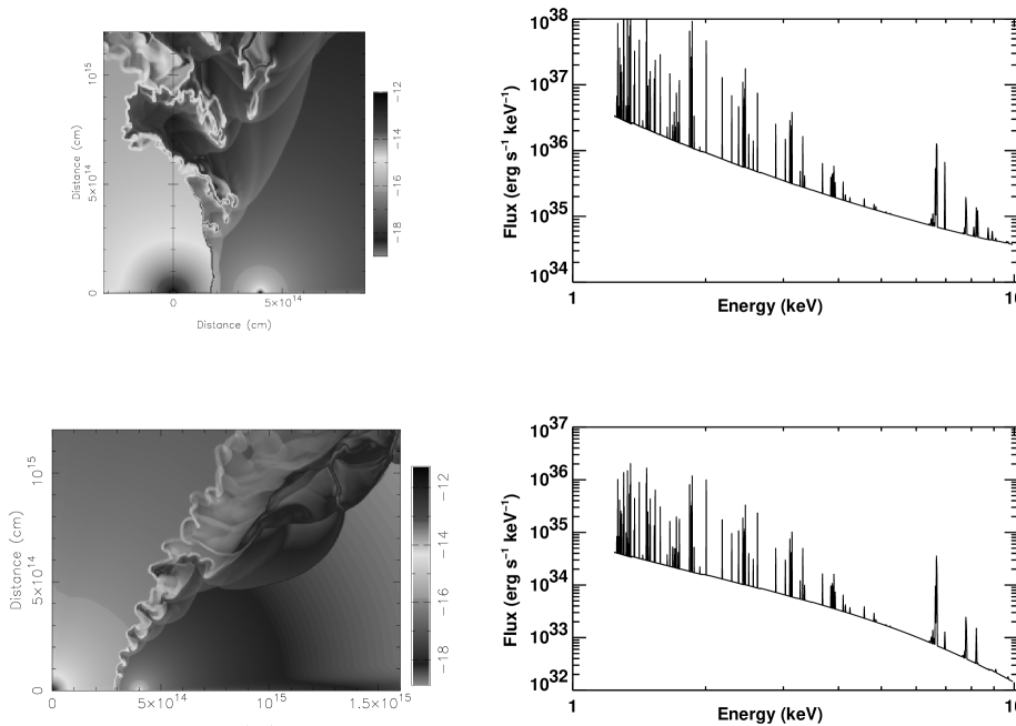
Figure 2: Hydrodynamic simulations and theoretical spectra of the colliding winds in $\eta$ Car. The top panels show the results from a model where the momentum of each wind is equal ($\eta=1$), whereas in the bottom panels the primary wind has a momentum 10 times greater than the secondary wind ($\eta=0.1$). In both cases a density plot (${\rm g\;cm^{-3}}$) from the hydrodynamical grid is shown on the left and the resulting intrinsic X-ray spectrum shown on the right (no absorption). On each hydrodynamical grid the primary star is located at (0,0) and the secondary star is at ($4.0\times 10^{14}$,0). The shape and structure of the shocked region varies with the momentum balance between the winds and the respective value of $\chi$ for each shocked wind. The full parameters used in these models were: upper panels - $\hbox{${\dot{M}}$}\,_{1}=10^{-3}\;\hbox{${\rm\hbox{${\rm\thinspace M_{\odot}}$}{\rm\thinspace yr}^{-1}\,}$}$, $\hbox{${\dot{M}}$}\,_{2}=10^{-4}\;\hbox{${\rm\hbox{${\rm\thinspace M_{\odot}}$}{\rm\thinspace yr}^{-1}\,}$}$, $v_{\infty_{1}}=500\;\hbox{${\rm{\rm\thinspace km}{\rm\thinspace s}^{-1}\,}$}$, $v_{\infty_{2}}=5000\;\hbox{${\rm{\rm\thinspace km}{\rm\thinspace s}^{-1}\,}$}$; lower panels - $\hbox{${\dot{M}}$}\,_{1}=3\times 10^{-4}\;\hbox{${\rm\hbox{${\rm\thinspace M_{\odot}}$}{\rm\thinspace yr}^{-1}\,}$}$, $\hbox{${\dot{M}}$}\,_{2}=10^{-5}\;\hbox{${\rm\hbox{${\rm\thinspace M_{\odot}}$}{\rm\thinspace yr}^{-1}\,}$}$, $v_{\infty_{1}}=500\;\hbox{${\rm{\rm\thinspace km}{\rm\thinspace s}^{-1}\,}$}$, $v_{\infty_{2}}=1500\;\hbox{${\rm{\rm\thinspace km}{\rm\thinspace s}^{-1}\,}$}$. The luminosity and shape of the X-ray spectrum are a direct consequence of these parameters.

The spectrum from each hydrodynamic model was averaged over 3 ‘snapshots’ each spaced by about 70 d. This is of order the wind dynamical timescale and serves to approximate a time-averaged spectrum. It is particularly important to adopt this approach for models where the wind collision region is very unstable since in these cases the flux can vary by greater than $\pm 50\%$ from one snapshot to the next. As already noted by Corcoran et al. (2001b ) no variability is seen during the $\approx 90\;{\rm ksec}$ exposure of the Chandra grating spectrum. This is to be expected, however, since the dynamical timescale is much longer. Two examples of ‘time-averaged’ synthetic spectra are shown in Fig. 2, next to density plots of the corresponding hydrodynamic calculation.

The synthetic spectra were calculated over the energy range 1.26–10 keV (10–1.26 $\AA$ respectively), and have a resolution of 0.005 $\AA$. The actual grating spectrum shows significant absorption below 1.5 keV and contains essentially no useful information below our lower limit of 1.26 keV. The spectral resolution of our synthetic spectra is approximately twice as high as the grating data that we model. Use of the Raymond-Smith plasma code implicitly assumes that the plasma is in thermal equilibrium. This is generally true for colliding wind binary systems (see Luo et al. LMM1990 (1990)) and is a good assumption for $\eta$ Car.

Figure 3: Variation in the spectral shape and normalization of the theoretical colliding winds spectra in $\eta$ Carinae. The top panel shows the variation with $\eta$ ($\hbox{${\dot{M}}$}\,_{2}=10^{-6}\;\hbox{${\rm\hbox{${\rm\thinspace M_{\odot}}$}{\rm\thinspace yr}^{-1}\,}$}$, $v_{\infty_{2}}=3000\;\hbox{${\rm{\rm\thinspace km}{\rm\thinspace s}^{-1}\,}$}$). The middle panel shows the variation with $\hbox{${\dot{M}}$}\,_{2}$ ($\eta=5.0$, $v_{\infty_{2}}=1500\;\hbox{${\rm{\rm\thinspace km}{\rm\thinspace s}^{-1}\,}$}$). The bottom panel shows the variation with $v_{\infty_{2}}$ ($\eta=0.1$, $\hbox{${\dot{M}}$}\,_{2}=10^{-5}\;\hbox{${\rm\hbox{${\rm\thinspace M_{\odot}}$}{\rm\thinspace yr}^{-1}\,}$}$).

2.2 Variations with $\eta$, $\hbox{${\dot{M}}$}\,_{2}$, and $v_{\infty_{2}}$

In Fig. 3 and the following subsections we reveal how the shape and normalization of the calculated spectra depend on the various free parameters of the grid.

2.2.1 Variation with $\eta$

Due to the low preshock velocity of the primary wind, the X-ray emission from the WWC is almost entirely from the shocked secondary wind. A greater fraction of the secondary wind passes into the wind collision zone as the relative momentum of the primary wind is increased, so we expect the luminosity to increase as $\eta$ decreases, as indeed the top panel of Fig. 3 shows. An important point, however, is that the shape of the spectra do not seem dependent on the value of $\eta$, contrary to our expectations before starting this study.

2.2.2 Variation with $\hbox{${\dot{M}}$}\,_{2}$

As we increase the mass-loss rate of the secondary star in our models, the kinetic power and the density of its wind also increase. Therefore, for a given wind momentum ratio, the rate of conversion of kinetic energy to thermal energy increases, as does the density of the postshock gas. Thus there is more available energy to radiate and a greater efficiency of radiation. Hence we should expect the X-ray luminosity to scale strongly with increasing $\hbox{${\dot{M}}$}\,_{2}$. This is indeed what we see in the middle panel of Fig. 3, where an order of magnitude increase in $\hbox{${\dot{M}}$}\,_{2}$ leads to an almost two order of magnitude increase in X-ray luminosity, indicating that the calculations in this panel are in the adiabatic regime ($L_{x}\propto\hbox{${\dot{M}}$}\,^{2}$; see Stevens et al. SBP1992 (1992)). However, there is no evidence for a softening of the spectrum with increasing $\hbox{${\dot{M}}$}\,_{2}$. This is again contrary to our initial expectations (note, however, the discussion in the next section).

2.2.3 Variation with $v_{\infty_{2}}$

If the preshock velocity of a wind is increased, the postshock temperature increases ($T\propto v^{2}$). Therefore we expect the model spectra to harden as the preshock velocity of the secondary wind is increased. Because the kinetic power of the wind increases we also expect the luminosity to increase. The variation of the spectrum with $v_{\infty_{2}}$ is shown in the bottom panel of Fig. 3. Here we find that our expectations are only partially met. The overall luminosity does increase with $v_{\infty_{2}}$, and the spectrum does harden between $v_{\infty_{2}}=1500-3000\;\hbox{${\rm{\rm\thinspace km}{\rm\thinspace s}^{-1}\,}$}$, but it softens between $v_{\infty_{2}}=3000-5000\;\hbox{${\rm{\rm\thinspace km}{\rm\thinspace s}^{-1}\,}$}$. An investigation into this surprising finding offers the following explanation.

For fixed $\eta$ and $\hbox{${\dot{M}}$}\,_{2}$, and variable $v_{\infty_{2}}$, the density of the wind varies as $\rho\propto\hbox{${\dot{M}}$}\,/v_{\infty_{2}}$. If $v_{\infty_{2}}$ is increased $\rho$ decreases, which reduces the radiative efficiency of the hot shocked gas near the stagnation point ($\dot{E}\propto n^{2}$), which acts to slightly suppress the hard flux. A plot of the average density against $T$ for $v_{\infty_{2}}=1500,\;3000,\;5000\;\hbox{${\rm{\rm\thinspace km}{\rm\thinspace s}^{-1}\,}$}$ also reveals that for $10^{6.3}<T<10^{7.4}$ the average density is higher when $v_{\infty_{2}}=5000\;\hbox{${\rm{\rm\thinspace km}{\rm\thinspace s}^{-1}\,}$}$ than when $v_{\infty_{2}}=3000\;\hbox{${\rm{\rm\thinspace km}{\rm\thinspace s}^{-1}\,}$}$, which tends to keep up the soft emission relative to the hard emission. This appears to be because there is some mixing at the interface between the primary and secondary wind, and the shocked primary wind is denser when $v_{\infty_{2}}=5000\;\hbox{${\rm{\rm\thinspace km}{\rm\thinspace s}^{-1}\,}$}$ ($\hbox{${\dot{M}}$}\,_{1}=3\times 10^{-4},\;{\mbox{6}\times 10^{-4}},\;10^{-3}\;\hbox{${\rm\hbox{${\rm\thinspace M_{\odot}}$}{\rm\thinspace yr}^{-1}\,}$}$ for $v_{\infty_{2}}=1500,\;3000,\;5000\;\hbox{${\rm{\rm\thinspace km}{\rm\thinspace s}^{-1}\,}$}$). The mixed gas tends to be at these intermediate temperatures.

Figure 4: Variation in the spectral shape and normalization for a very fast secondary wind ($v_{\infty_{2}}=5000\;\hbox{${\rm{\rm\thinspace km}{\rm\thinspace s}^{-1}\,}$}$) and a fixed wind momentum ratio ($\eta=0.1$). As $\hbox{${\dot{M}}$}\,_{2}$ increases the spectrum becomes slightly harder.

The overall net effect is that the emission from the hot gas is suppressed relative to the cooler gas, which softens the spectrum from the model with $v_{\infty_{2}}=5000\;\hbox{${\rm{\rm\thinspace km}{\rm\thinspace s}^{-1}\,}$}$ relative to the model with $v_{\infty_{2}}=3000\;\hbox{${\rm{\rm\thinspace km}{\rm\thinspace s}^{-1}\,}$}$. These inferences are supported by spectra calculated with $v_{\infty_{2}}=5000\;\hbox{${\rm{\rm\thinspace km}{\rm\thinspace s}^{-1}\,}$}$ and $\eta=0.1$, and variable $\hbox{${\dot{M}}$}\,_{2}$ (Fig. 4). This shows that the spectrum hardens as $\hbox{${\dot{M}}$}\,_{2}$ increases from $10^{-6}\;\hbox{${\rm\hbox{${\rm\thinspace M_{\odot}}$}{\rm\thinspace yr}^{-1}\,}$}$ to $10^{-4}\;\hbox{${\rm\hbox{${\rm\thinspace M_{\odot}}$}{\rm\thinspace yr}^{-1}\,}$}$ (the spectral index $\alpha$, where $F_{\nu}\propto\nu^{\alpha}$, increases by about 0.1). This is what we expect from our prior inferences since a higher $\hbox{${\dot{M}}$}\,_{2}$ helps to make postshock gas with a preshock velocity of $v_{\infty_{2}}=5000\;\hbox{${\rm{\rm\thinspace km}{\rm\thinspace s}^{-1}\,}$}$ somewhat more efficient at radiating. In summary, we find that varying $\hbox{${\dot{M}}$}\,_{2}$ can actually have a small effect on the shape of the spectrum in some parts of parameter space, as well as the more obvious and much greater effect on the luminosity. The power of $\hbox{${\dot{M}}$}\,_{2}$ on affecting the spectral shape is, however, much less than that of $v_{\infty_{2}}$, which is the primary influence.

2.2.4 Summary of Spectral Dependence on $\eta$, $\hbox{${\dot{M}}$}\,_{2}$, and $v_{\infty_{2}}$

For the models investigated in this paper, we find that the spectral shape is i) insensitive to the value of $\eta$, ii) can harden slightly as $\hbox{${\dot{M}}$}\,_{2}$ increases (in other parts of parameter space, e.g. strongly radiative shocks, it may soften with increasing $\hbox{${\dot{M}}$}\,_{2}$), and iii) generally hardens with increasing $v_{\infty_{2}}$, but can sometimes soften. The luminosity increases with i) decreasing $\eta$ (since $\eta$ Car is unusual in the sense that there is no discernible contribution to the X-rays from the shocked primary wind, bar mixing), ii) increasing $\hbox{${\dot{M}}$}\,_{2}$, and iii) increasing $v_{\infty_{2}}$.

2.3 The Spectral Grid

The synthetic spectra were input into a FITS-style ‘Table’ model for use with the XSPEC data-analysis package, as specified by Arnaud (A1999 (1999)). The fitting procedure within XSPEC is able to interpolate between the parameter values on the spectral grid so that best-fit values of $\hbox{${\dot{M}}$}\,_{2}$ etc. are obtained from fitting the Chandra data. In the $2-10$ keV band, the intrinsic luminosity on our grid ranges from $1.8\times 10^{31}\;\hbox{${\rm{\rm\thinspace erg}{\rm\thinspace s}^{-1}\,}$}$ to $1.6\times 10^{37}\;\hbox{${\rm{\rm\thinspace erg}{\rm\thinspace s}^{-1}\,}$}$, which brackets the observationally determined value of $4\times 10^{34}\;\hbox{${\rm{\rm\thinspace erg}{\rm\thinspace s}^{-1}\,}$}$ (Corcoran et al. 2001b ).

3 Fits to the Chandra grating spectrum

We compared the model intrinsic colliding wind spectra with the observed grating spectrum allowing the mass-loss rate and wind terminal velocity of the companion to vary. We in addition included absorption from a cool overlying medium to simulate the combined absorption of the circumstellar (nebular) material in the Homunculus, the ISM, and the wind from the companion (all of which may contribute to the X-ray absorption at some level). Since the stellar wind absorption depends on the companion’s mass-loss rate (at the phase of the Chandra observation) for consistency we should model this component of the absorption directly, but this is beyond the scope of the present paper. Because of the low number of counts per spectral bin in the high-resolution grating spectrum, and because background does not contribute significantly to the observed spectrum at energies above 2 keV, we fit the gross spectrum using the C-statistic (Cash C1979 (1979)), which is appropriate for Poisson-distributed data.

The fact that the shapes of our model spectra are not dependent on the value of $\eta$ introduces a degeneracy into our grid as both $\eta$ and $\hbox{${\dot{M}}$}\,_{2}$ primarily influence the normalization of the spectra. This means that various combinations of $\eta$ and $\hbox{${\dot{M}}$}\,_{2}$ can provide similar quality fits to the data. However, it is possible to obtain an estimate for $\eta$ from the duration of the lightcurve minimum ($\approx 100$ d). To do this we have constructed a simple model of the observed X-ray emission. We assume that the intrinsic flux varies as $1/D$, and that the absorption from the shock apex along the line of sight is negligible when viewing through the less dense secondary wind, but total when viewing through the very dense primary wind. We use the latest orbital parameters (Corcoran et al. 2001a ) and assume that the skew angle of the shock cone from the orbital velocity, $v_{\rm orb}$, is $\delta\simeq\arctan(v_{\rm orb}/v_{\infty_{1}})$. Fig. 5 shows the results, scaled so that $L_{x}=1$ at periastron. The skew of the shock breaks the symmetry of the observed emission so that the post-minimum flux is lower than the pre-minimum flux, as observed. The duration of the minimum decreases with increasing $\eta$ (for $\eta=0.1,0.2,0.3$ the duration is $133,92,71\;{\rm d}$), and is best matched by $\eta\approx 0.2$. Therefore we adopt this value for the rest of our analysis.

Figure 5: The duration of the X-ray minimum predicted from simple models. The wind momentum ratio in the three models shown is $\eta=0.2,1.0,5.0$ (solid, dots, dashes), which gives a duration of $92,33,16\;{\rm d}$ respectively. The observed duration is $\approx 100\;{\rm d}$, so the data is best approximated by $\eta=0.2$.

We attempted to fit the grid of synthetic colliding wind spectra to the observed MEG +1 order spectrum. We also constrained the spectrum normalization to lie between 0.8 and 1.2, which fixes the distance to the star between 2300 and 1900 pc, close to the canonical distance of 2100 pc. In Fig. 6 we show the best fit interpolated spectrum from our grid in the range $1.5-7.5$ keV. Fig. 7 shows a close-up of the fit to the Si and S emission lines between $1.8-2.8$ keV. Both figures demonstrate the excellent agreement found between the data and the models and highlight the progress made in both the observational and theoretical study of colliding winds over the last 10 years. The continuum shape and level from the models matches closely that of the data. All strong lines (and most weak ones) which appear in the observed spectrum are matched also in the best fit. This means that the temperature distribution seen in the grating spectrum is matched by the model. However most of the strong lines are significantly overpredicted by the model fit. This discrepancy is in the opposite sense to the fit results from simple one- and two-temperature Raymond-Smith models, and is perhaps revealing that our assumption of solar abundances needs to be modified. The best fit parameters are summarized in Table 2.

Figure 6: Best fit to the Chandra grating spectrum. The fit parameters were $\hbox{${\dot{M}}$}\,_{2}=0.98\times 10^{-5}\;\hbox{${\rm\hbox{${\rm\thinspace M_{\odot}}$}{\rm\thinspace yr}^{-1}\,}$}$, $v_{\infty_{2}}=3000\;\hbox{${\rm{\rm\thinspace km}{\rm\thinspace s}^{-1}\,}$}$, $\eta=0.2$, $N_{\rm H}=7.7\times 10^{22}\;{\rm\thinspace cm}^{-2}$, and the overall normalization was 1.16. If we take $v_{\infty_{1}}=600\;\hbox{${\rm{\rm\thinspace km}{\rm\thinspace s}^{-1}\,}$}$, this implies that $\hbox{${\dot{M}}$}\,_{1}=2.5\times 10^{-4}\;\hbox{${\rm\hbox{${\rm\thinspace M_{\odot}}$}{\rm\thinspace yr}^{-1}\,}$}$. As seen from the figure, the continuum level is very well fitted by the interpolated model.

Figure 7: Zoomed in view of Fig. 6 showing the spectrum in the $1.8-2.8$ keV region. The lines are identified as either S or Si, and from left to right are: Si XIII triplet (1.839, 1.854, 1.865 keV), Si XIV (2.006 keV), Si XIII (2.182 keV), Si XIV (2.375 keV), S XV triplet (2.429, 2.447 keV), S XVI (2.622 keV). The fit to the S lines is very good, while the model slightly overpredicts the emission from the Si lines, perhaps indicating that the Si abundance is slightly sub-solar.

Table 2: The best fit parameters from the fit of the spectral grid to the grating data. We fix the terminal velocity of the primary wind at $500\;\hbox{${\rm{\rm\thinspace km}{\rm\thinspace s}^{-1}\,}$}$, the stellar separation at $D=4.0\times 10^{14}\;{\rm cm}$, and the wind momentum ratio ($\eta$) at 0.2, and allow $\hbox{${\dot{M}}$}\,_{2}$, $v_{\infty_{2}}$, $N_{\rm H}$ and the normalization to vary. Solar abundances were assumed, and a cold external absorbing column was applied. The resultant normalization is very close to 1.0, which indicates that the model and the values of $D$ and $\eta$ are sensible. Alternatively, it implies that our assumed distance to $\eta$ Car is too far by a factor of 1.077, if we imagine this as the sole source of discrepancy. This would revise the source distance down to 2.1/1.077 = 1.95 kpc, which is well inside of observational uncertainties. The implied mass-loss rate of the primary star from our fit is $\hbox{${\dot{M}}$}\,_{1}=2.5\times 10^{-4}\;\hbox{${\rm\hbox{${\rm\thinspace M_{\odot}}$}{\rm\thinspace yr}^{-1}\,}$}$.

Parameter	Value
$\eta$	0.2 (fixed)
$\hbox{${\dot{M}}$}\,_{2}\;(\hbox{${\rm\hbox{${\rm\thinspace M_{\odot}}$}{\rm\thinspace yr}^{-1}\,}$})$	$0.98^{+0.09}_{-0.08}\times 10^{-5}$
$v_{\infty_{2}}\;(\hbox{${\rm{\rm\thinspace km}{\rm\thinspace s}^{-1}\,}$})$	$3000^{+350}_{-340}$
$N_{\rm H}\;({\rm cm^{-2}})$	$7.68^{+0.17}_{-0.17}\times 10^{22}$
Normalization	1.16

4 Conclusions

In this paper our aim has been to test the binary hypothesis of $\eta$ Car by directly fitting its X-ray spectrum using a grid of spectra calculated from hydrodynamical models of the wind-wind collision. While our analysis does not prove that it is a binary, we find that the colliding wind emission model naturally provides for the range of ionization seen in the emission line grating spectrum for reasonable values of the wind parameters. We have not shown that it is inconsistent with emission from a single star, but have noted that it is unlike any of the other single stars observed so far at high energies and dispersion.

The technique applied in this paper has only been demonstrated once before and is the first time that it has been used with a high quality grating spectrum. Due to the low velocity of the primary wind ($\approx 500\hbox{${\rm{\rm\thinspace km}{\rm\thinspace s}^{-1}\,}$}$), most of the observed X-ray emission arises from the shocked wind of the companion star. We find it difficult therefore to fit both $\hbox{${\dot{M}}$}\,_{1}$ and $v_{\infty_{1}}$ as free parameters. However, the duration of the observed X-ray minimum can be used to estimate the wind momentum ratio of the stars, $\eta$. With $\eta$ fixed at 0.2, and $\hbox{${\dot{M}}$}\,_{2}$, and $v_{\infty_{2}}$ as free parameters, we are able to obtain a good fit to the data.

We find that the mass-loss rate of the companion is $\hbox{${\dot{M}}$}\,_{2}\approx 10^{-5}\;\hbox{${\rm\hbox{${\rm\thinspace M_{\odot}}$}{\rm\thinspace yr}^{-1}\,}$}$ and the terminal velocity of its wind is $v_{\infty_{2}}\approx 3000\;\hbox{${\rm{\rm\thinspace km}{\rm\thinspace s}^{-1}\,}$}$. These values suggest that the companion is probably an Of supergiant (O-stars with similar wind parameters - e.g. HD 15570 (O4If), HD 93129A (O3If), HD 93250 (O3Vf), HD 151804 (O8If), and Cyg OB2 #9 (O5If) - are listed in Howarth & Prinja HP1989 (1989)), or is possibly a WR star. The velocity of the primary wind has been determined to lie in the range $500-700\;\hbox{${\rm{\rm\thinspace km}{\rm\thinspace s}^{-1}\,}$}$ (e.g. Hillier et al. HDIG2001 (2001)). Hence our fit implies a primary mass-loss rate of $\hbox{${\dot{M}}$}\,_{1}\approx 2.5\times 10^{-4}\;\hbox{${\rm\hbox{${\rm\thinspace M_{\odot}}$}{\rm\thinspace yr}^{-1}\,}$}$. From the uncertainty in the value of $\eta$, and the interpolation on our grid, we estimate the uncertainty on our derived value for $\hbox{${\dot{M}}$}\,_{1}$ as approximately a factor of 2.

Our best-fit estimate of $\hbox{${\dot{M}}$}\,_{1}$ is smaller than typically inferred (cf. Davidson & Humphreys DH1997 (1997); Hillier et al. HDIG2001 (2001)) However, we note that a lower mass-loss rate for the primary star can reduce some of the problems noted by Hillier et al. (HDIG2001 (2001)) who fitted a value as high as $10^{-3}\;\hbox{${\rm\hbox{${\rm\thinspace M_{\odot}}$}{\rm\thinspace yr}^{-1}\,}$}$. In particular, the models of Hillier et al. (HDIG2001 (2001)) suffered from absorption components that were too strong and electron-scattering wings which were overestimated. Both indicate that their chosen mass-loss rate is too high. Paradoxically both the H$\alpha$ and H$\beta$ emission lines were weaker than observed, indicating that their mass-loss rate is too low. However, it is well known that the wind collision zone can be a strong source of emission lines (e.g. HD 5980, Moffat et al. M1998 (1998)), which would resolve this problem. Their inferred minimum column density is also larger than the observed X-ray value, again implying an overestimate of $\hbox{${\dot{M}}$}\,_{1}$. To increase the mass-loss rate of the primary towards the value estimated by Hillier et al. (HDIG2001 (2001)), we require either a reduction in the wind velocity to $\approx 100\;\hbox{${\rm{\rm\thinspace km}{\rm\thinspace s}^{-1}\,}$}$, which in turn is in conflict with previous estimates, or a reduction in the wind momentum ratio to $\eta\mathrel{\hbox to0.0pt{\lower 3.0pt\hbox{$\sim$}\hss}\raise 2.0pt\hbox{$<$}}0.1$, which is in conflict with the observed duration of the X-ray minimum. Finally, it is worth noting that our results indicate a value for $\hbox{${\dot{M}}$}\,_{1}$ which is closer to the value inferred for the Pistol star ($\hbox{${\dot{M}}$}\,\approx 4\times 10^{-4}\;\hbox{${\rm\hbox{${\rm\thinspace M_{\odot}}$}{\rm\thinspace yr}^{-1}\,}$}$; Figer et al. F1998 (1998)), an extreme early-type star with similarities to $\eta$ Car.

Since current observations and theoretical modelling of the optical spectrum are unable to determine the effective temperature and the stellar radius of the primary without first determining $\hbox{${\dot{M}}$}\,_{1}$ (cf. Hillier et al. HDIG2001 (2001)), our independent estimate may prove to be extremely useful in this regard. It will be interesting to see if the results from this paper are consistent with future X-ray observations, and whether estimates of $\hbox{${\dot{M}}$}\,_{1}$ from observations at X-ray and other wavelengths can be reconciled. Future X-ray grating observations should also help us to fix the value of the wind momentum ratio more accurately.

As the secondary wind dominates the X-ray spectrum, and its terminal velocity appears to be high ($\approx 3000\;\hbox{${\rm{\rm\thinspace km}{\rm\thinspace s}^{-1}\,}$}$), we should expect to see signs of Doppler broadening and shifts in the line profiles. While there is little evidence for this in the current spectrum, other orbital phases may be more favourable in this regard. The addition of Doppler effects has already been incorporated in modelled X-ray spectra (Pittard et al. in preparation), and should provide further information on wind velocities and the structure of the wind-wind collision region.

The over-prediction of the X-ray lines in our models perhaps indicates that the companion has sub-solar abundances, which favours an O-type over a WR classification, although we would need to perform a more detailed analysis to confirm this possibility. As the primary has slightly enhanced abundances of C and N compared to solar, this suggests that to date there has been no mass exchange between the stars. Lamers et al. (LLPW1998 (1998)) suggested that the star which dominates the UV GHRS spectrum is not the star which ejected the nebula since the abundances in the GHRS spectrum are not as evolved as the abundances in the nebula (which are indicative of CNO-cycle products). As the UV bright source is probably the companion (Hillier et al. HDIG2001 (2001)) this indicates that it was the primary which ejected the nebula. There are also some caveats about the analysis in Lamers et al. (LLPW1998 (1998)) since strong C lines (which Lamers et al. took to indicate normal CNO abundances in the GHRS spectrum) also appear in stars known to be deficient in C (see the discussion in Hillier et al. HDIG2001 (2001)). It is also interesting to note that the UV spectrum brightened in 1999.1 vs. 1998.2, which is suggestive of an eclipse of the UV source near periastron in 1998. In conclusion, the high energy photons (UV and X-ray) seem to be telling us about the companion.

We emphasize that contrary to the vast majority of colliding wind systems, our X-ray analysis of $\eta$ Car primarily probes the conditions of the shocked wind of the companion. X-ray observations of $\eta$ Car are therefore unique in this regard since at other wavelengths (with the possible exception of the far UV) the wind of the primary dominates the observed phenomena. While our analysis has for the first time provided a direct estimate of the wind parameters of the companion star, relating these to the stellar parameters (mass, radius, luminosity) of the companion star requires more work. It is anticipated that the continued multi-wavelength study of $\eta$ Car through and beyond the next periastron passage will further reveal the hidden secrets of this most enigmatic system.

- (1) Arnaud K.A., 1999, OGIP Memo 92-009
- (2) Blondin J.M., Kallman T.R., Fryxell B.A., Taam R.E., 1990, ApJ, 356, 591
- (3) Cash W., 1979, ApJ, 228, 939
- (4) Cherepashchuk A.M., 1976, Soviet Astr. Lett., 2, 138
- (5) Colella P., Woodward P.R., 1984, JCP, 54, 174
- (6) Corcoran M.F., Ishibashi K., Swank J.H., Davidson K., Petre R., Schmitt J.H.M.M., 1997, Nature, 390, 587
- (7) Corcoran M.F., Fredericks A.C., Petre R., Swank J.H., Drake S.A., 2000, ApJ, 545, 420
- (8) Corcoran M.F., Ishibashi K., Swank J.H., Petre R., 2001a, ApJ, 547, 1034
- (9) Corcoran M.F., Rawley G.L., Swank J.H., Petre R., 1995, ApJ, 445, L121
- (10) Corcoran M.F., et al. , 2001b, ApJ, 562, 1031
- (11) Damineli A., 1996, ApJ, 460, L49
- (12) Damineli A., Conti P.S., Lopes D.F., 1997, New Astr. 2, 107
- (13) Damineli A., Kaufer A., Wolf B., Stahl O., Lopes D.F., Araújo F.X., 2000, ApJ, 528, L101
- (14) Davidson K., Humphreys R.M., 1997, ARA&A, 35, 1
- (15) Davidson K., Ishibashi K., Corcoran M.F., 1998, New Astr., 3, 241
- (16) Davidson K., Ishibashi K., Gull T.R., Humphreys R.M., Smith N., 2000, ApJ, 530, L107
- (17) Duncan R.A., et al. , 1995, ApJ, 441, L73
- (18) Duncan R.A., White S.M., Reynolds J.E., Lim J., 1999, ASP Conf. Ser. 179, Eta Carinae at the Millenium, ed J.A. Morse, R.M., Humphreys, A. Damineli (San Francisco: ASP), 54
- (19) Eichler D., Usov V., 1993, ApJ, 402, 271
- (20) Figer D.F., Najarro F., Morris M., McLean I.S., Geballe T.R., Ghez A.M., Langer N., 1998, ApJ, 506, 384
- (21) Gallager J.S., 1989, Proc. of 113 IAU Colloquium, Physics of Luminous Blue Variables (Kluwer Academic Publishers), 185
- (22) Guzik J.A., Cox A.N., Despain K.M., 1999, ASP Conf. Ser. 179, Eta Carinae at the Millenium, ed J.A. Morse, R.M., Humphreys, A. Damineli (San Francisco: ASP), 54
- (23) Hillier D.J., Davidson K., Ishibashi K., Gull T., 2001, ApJ, 553, 837
- (24) Howarth I.D., Prinja R.K., 1989, ApJSS, 69, 527
- (25) Ishibashi K., et al. , 1999, ApJ, 524, 983
- (26) Kahn S.M., et al. , 2001, A&A, 365, L312
- (27) Lamers, H.J.G.L.M., 1997, ASP Conf. Ser. 120, Luminous Blue Variables: Massive Stars in Transition, ed A. Nota, H.J.G.L.M. Lamers (San Francisco: ASP), 76
- (28) Lamers, H.J.G.L.M., Livio M., Panagia N., Walborn N.R., 1998, ApJ, 505, L131
- (29) Langer N., 1997, ASP Conf. Ser. 120, Luminous Blue Variables: Massive Stars in Transition, ed A. Nota, H.J.G.L.M. Lamers (San Francisco: ASP), 83
- (30) Langer N., Hamann W.-R., Lennon M., Najarro F., Pauldrach A.W.A., Puls J., 1994, A&A, 290, 819
- (31) Leitherer C., et al. , 1994, ApJ, 428, 292
- (32) Luo D., McCray R., Mac Low M-M., 1990, ApJ, 362, 267
- (33) Maeder A., Meynet G., 2001, A&A, 373, 555
- (34) Mewe R., Kaastra J.S., Liedahl D.A., 1995, Legacy, 6, 16
- (35) Moffat A.F.J., et al. , 1998, ApJ, 497, 896
- (36) Morse J.A., Davidson K., Smith N., 1999, AJ 116, 2443
- (37) Nota A., Pasquali A., Drissen L., Leitherer C., Robert C., Moffat A.F.J., Schmutz W., 1996, ApJS, 102, 383
- (38) Prilutskii O.F., Usov V.V., 1976, Soviet Astr., 20, 2
- (39) Rauw G., Stevens I.R., Pittard J.M., Corcoran M.F., 2000, MNRAS, 316, 129
- (40) Raymond J.C., Smith B.W., 1977, ApJS, 35, 419
- (41) Pittard J.M., 2000, PhD. Thesis, University of Birmingham, UK
- (42) Pittard J.M., Stevens I.R., Corcoran M.F., Ishibashi K., 1998, MNRAS, 299, L5
- (43) Schulz N.S., Canizares C.R., Huenemoerder D., Lee J.C., 2000, ApJ, 545, L135
- (44) Stevens I.R., Blondin J.M., Pollock A.M.T., 1992, ApJ, 386, 285
- (45) Stevens I.R., Corcoran M.F., Willis A.J., et al. , 1996, MNRAS, 283, 589
- (46) Stothers S., Chin C.-W., 1993, ApJ, 408, L85
- (47) Strickland D.K., Stevens I.R., 1998, MNRAS, 297, 747
- (48) Tsuboi Y., Koyama K., Sakano M., Petre R., 1997, PASJ, 49, 85
- (49) Usov V.V., 1992, ApJ, 389, 635
- (50) Viotti R., 1995, Rev. Mex. AA, 2, 10
- (51) Waldron W., Cassinelli J.P., 2001, ApJ, 548, L45
- (52) Weis K., Duschl W.J., Bomans D.J., 2001, A&A, 367, 566
- (53) Zethson T., Johansson S., Davidson K., Humphreys R.M., Ishibashi K., Ebbets D., 1999, A&A, 344, 211
- (54) Zhekov S.A., Skinner S.L., 2000, ApJ, 538, 808