Effects of Relativistic Expansion on the Late-time Supernova Light Curves

Abstract

The effects of relativistic expansion on the late-time supernova light curves are investigated analytically, and a correction term to the (quasi-)exponential decay is obtained by expanding the observed flux in terms of $\beta$, where $\beta$ is the maximum velocity of the ejecta divided by the speed of light $c$. It is shown that the Doppler effect brightens the light curve owing to the delayed decay of radioactive nuclei as well as to the Lorentz boosting of the photon energies. The leading correction term is quadratic in $\beta$, thus being proportional to $E_{\rm k}/(M_{\rm ej}c^{2})$, where $E_{\rm k}$ and $M_{\rm ej}$ are the kinetic energy of explosion and the ejecta mass. It is also shown that the correction term evolves as a quadratic function of time since the explosion. The relativistic effect is negligibly small at early phases, but becomes of considerable size at late phases. In particular, for supernove having a very large energy(hypernova) or exploding in a jet-like or whatever non-spherical geometry, ⁵⁶Ni is likely to be boosted to higher velocities and then we might see an appreciable change in flux. However, the actual size of deviation from the (quasi-)exponential decay will be uncertain, depending on other possible effects such as ionization freeze-out and contributions from other energy sources that power the light curve.

1 Introduction

It has long been recognized that the radiative transfer in supernova(SN) ejecta should be treated relativistically to account for the high velocities achieved in its outermost layers. However, it is only in the last decade that the first numerical codes for radiative transfer that take relativistic effects into account were developed and applied to transfer problems in SN ejecta. At early times of explosion, the energy of photons emitted from the photosphere of SN ejecta is greatly enhanced by the Doppler effect. As time goes on and the photosphere recedes towards the center of ejecta, the degree of the enhancement decreases, and eventually the resultant light curve(LC) is expected to follow an (quasi-)exponential deposition curve due to radioactive decays. However, there are several factors that cause the late-time LCs deviate from the radioactive decay curve. One possibility is the flattening of LCs owing to the so-called ionization freeze-out effect, as first pointed out by Fransson & Kozma (1993) for the late-time LC of SN 1987A. Another one is the signatures of contributions from other energy sources such as possible pulsar activity and circumstellar interaction as have been discussed by previous works.

In this Letter, I would like to point out that late-time SN LCs may show a deviation from radioactive decay curves as a result of the relativistic Doppler effect. In particular, for very energetic SNe or what are called hypernovae(HNe), the relativistic effect would be very important since the maximum velocity near the surface of ejecta reaches a significant fraction of the speed of light. It will be shown that the Doppler effect makes a LC brighter due to the Lorentz boosting, but at the same time the light-traveling-time effect and a pure-relativistic effect delay the decay of radioactive nuclei, thus tending to make the LC even brighter at late phases. The net result is determined by the sum of these two effects. Late-time LCs provide direct information to determine the ⁵⁶Ni masses ejected by SNe. Therefore, its precise determination is of great importance for studies of SN explosion mechanism and chemical evolution of galaxies. In this Letter, we study the relativistic effect on the late-time LCs and estimate the size of the correction to the (quasi-)exponential decay for ordinary SNe and HNe. For simplicity, we use the approximation that energy input from radioactivity is emitted as optical photons on the spot and carried away from the SN ejecta free of absorption.

2 Light Curves

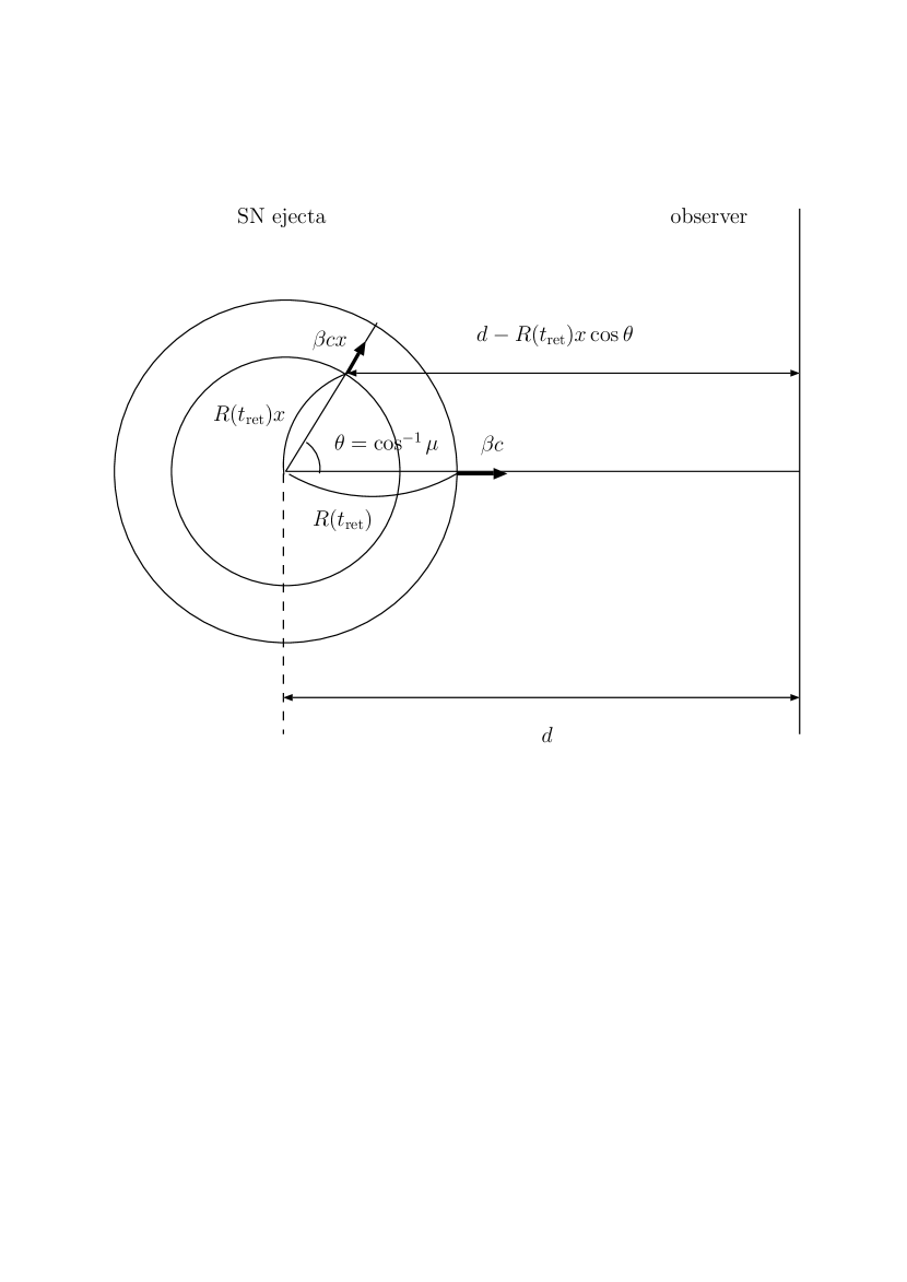
Figure 1: Schematic picture showing the position of a volume element of SN ejecta at a retarded time $t_{\rm ret}$.

We consider a spherically symmetric SN ejecta that expands homologously, so that its radius is given by $R(t)=R_{0}+\beta ct$ as a function of time $t$ after explosion, where $R_{0}$ is the initial radius, $\beta c$ is the surface velocity, and $c$ is the speed of light. Let us introduce the radial and azimuthal coordinates, $x$ and $\mu$, as shown in Figure 1, to designate volume elements of ejecta, such that $x$ runs from 0 to 1 outwards and that $\mu$ is the cosine of angle $\theta$ made between radial direction and the line of sight.

The flux of photons received by an observer at time $t$ is the sum of the emissions from the volume element at a retarded time $t_{\rm ret}$, $dV=2\pi R(t_{\rm ret})^{3}x^{2}dxd\mu$, where $t_{\rm ret}$ is defined by

$$c(t-t_{\rm ret}) = d-R(t_{\rm ret})x\cos\theta$$ (1)

$$\simeq d-c\beta\mu xt_{\rm ret}$$

and $d$ is the distance between the SN and the observer. We used the fact that the initial hydrodynamical time scale is short compared to the elapsed time considered, $R_{0}/\beta c<<t$. Solving equation (1) in terms of $t_{\rm ret}$, we obtain

$$t_{\rm ret}=\displaystyle\frac{t-d/c}{1-\beta\mu x}.$$ (2)

Let us define the frequency-integrated emissivity $j$ as the total energy of photons emitted per unit volume, unit time, and unit solid angle. Then, the emissivity in the rest frame in the direction toward the observer $j(x,\mu,t_{\rm ret})$ is related to that of the comoving frame $j_{c}$ such that

$$j(x,\mu,t_{\rm ret})=\displaystyle\frac{j_{\rm c}(x,\mu,t_{\rm ret,c})}{\gamma_{x}^{3}(1-\beta\mu x)^{3}},$$ (3)

where $\gamma_{x}=(1-\beta^{2}x^{2})^{-1/2}$ and $t_{\rm ret,c}=t_{\rm ret}/\gamma_{x}$ is the retarded time in the comoving frame (e.g.,Rybicki & Lightman, 1979). We assume that the radiative loss from the ejecta is balanced by the energy input due to radioactive decay and that the emissivity in the comoving frame is isotropic. Then, $j_{c}$ is written as

$$j_{\rm c}(x,\mu,t_{\rm ret,c})=\frac{1}{4\pi}f\epsilon\displaystyle\frac{n_{\rm c}(x,t_{\rm ret})}{\tau},$$ (4)

where $n_{c}$ is the number density of radioactive nuclei in the comoving frame, $\tau$ is its decay time, $\epsilon$ is the energy available per decay, and $f$ is the deposition fraction. The total number of radioactive nuclei in a volume element $\Delta V$, $\gamma_{x}n_{\rm c}\Delta V$, obeys the decay law given by

$$\displaystyle\frac{\partial}{\partial t_{\rm ret,c}}(\gamma_{x}n_{\rm c}\Delta V)=-\displaystyle\frac{\gamma_{x}n_{\rm c}\Delta V}{\tau},$$ (5)

or

$$\displaystyle\frac{\partial}{\partial t_{\rm ret}}(n_{\rm c}\Delta V)=-\displaystyle\frac{n_{\rm c}\Delta V}{\gamma_{x}\tau},$$ (6)

which has a solution

$$n_{\rm c}(x,t_{\rm ret}) = \displaystyle\frac{\Delta V(0)}{\Delta V(t_{\rm ret})}n_{\rm c}(x,0)e^{-\displaystyle\frac{t_{\rm ret}}{\gamma_{x}\tau}}=\left(\displaystyle\frac{R_{0}}{R(t_{\rm ret})}\right)^{3}n_{\rm c}(x,0)e^{-\displaystyle\frac{t_{\rm ret}}{\gamma_{x}\tau}}$$ (7)

$$= \left(\displaystyle\frac{R_{0}}{R(t_{\rm ret})}\right)^{3}\displaystyle\frac{n(x,0)}{\gamma_{x}}e^{-\displaystyle\frac{t_{\rm ret}}{\gamma_{x}\tau}}.$$

Using equation (7) in equation (4), we obtain

$$j_{\rm c}(x,\mu,t_{\rm ret,c})=\left(\displaystyle\frac{R_{0}}{R(t_{\rm ret})}\right)^{3}\frac{f\epsilon}{4\pi}\displaystyle\frac{n(x,0)}{\gamma_{x}\tau}e^{-\displaystyle\frac{t_{\rm ret}}{\gamma_{x}\tau}}.$$ (8)

In equating the energy emitted in a time $dt_{\rm ret}$ by a volume element at $x,\mu$ and time $t_{\rm ret}$, $dV(x,\mu,t_{\rm ret})$, with the corresponding energy passing through a normal area $\Delta S$ at the observer during time $dt$, $\Delta SdF(t)dt$, we have

$$dF(t)dt\Delta S=j(x,\mu,t_{\rm ret})dt_{\rm ret}dV(x,\mu,t_{\rm ret})\Delta\Omega,$$ (9)

where $dF(t)$ is the differential flux corresponding to the volume element and $\Delta\Omega$ is the solid angle subtended for the area $\Delta S$ by the volume element, and thus $\Delta S=d^{2}\Delta\Omega$. Adding up contributions by all the volume elements, we have the observed flux at time $t$,

$$F(t) = \frac{1}{d^{2}}\int\displaystyle\frac{\partial t_{\rm ret}}{\partial t}j(x,\mu,t_{\rm ret})dV$$ (10)

$$= \frac{1}{4\pi d^{2}}\displaystyle\frac{fN_{\rm tot}\epsilon}{\tau}\int_{0}^{1}dx3x^{2}\tilde{n}(x)\times\frac{1}{2}\int_{-1}^{1}d\mu\displaystyle\frac{1}{\gamma_{x}^{4}(1-\beta\mu x)^{4}}\exp\left[-\displaystyle\frac{\left(t-d/c\right)/\tau}{\gamma_{x}(1-\beta\mu x)}\right].$$

Here, $\tilde{n}(x)=n(x,0)/\bar{n}$ is the dimensionless number density of the radioactive nuclei and $N_{\rm tot}=(4\pi/3)R_{0}^{3}\bar{n}$ is its total number at $t=0$, where $\bar{n}$ is the average number density defined as

$$\bar{n}\equiv\displaystyle\frac{\displaystyle\int_{0}^{1}n(x,0)x^{2}dx}{\displaystyle\int_{0}^{1}x^{2}dx}=3\int_{0}^{1}n(x,0)x^{2}dx,$$ (11)

and thus $\tilde{n}$ is normalized such that

$$\int_{0}^{1}3x^{2}\tilde{n}(x)dx=1.$$ (12)

In deriving equation (10), it is assumed that $f$ is constant throughout the ejecta for simplicity. This holds for ⁵⁶Co decay at sufficiently late times when the deposition is primarily due to $e^{+}$ decay, and even for general cases if only the effect of a varying $f$ is incorporated into $\tilde{n}$. Using the variable $y\equiv\gamma_{x}^{-1}(1-\beta\mu x)^{-1}$ instead of $\mu$, the equation (10) is rewritten as

$$F(t)=\frac{1}{4\pi d^{2}}\displaystyle\frac{fN_{\rm tot}\epsilon}{\tau}\int_{0}^{1}dx3x^{2}\tilde{n}(x)f(\beta,x,X),$$ (13)

where

$$f(\beta,x,X)=\frac{1}{2\gamma_{x}\beta x}\int_{a(\beta,x)}^{b(\beta,x)}y^{2}e^{-Xy}dy,$$ (14)

$\displaystyle{X\equiv\frac{1}{\tau}\left(t-\displaystyle\frac{d}{c}\right),}$  and $a(\beta,x),b(\beta,x)$ are given by

$$a(\beta,x)=\left(\frac{1-\beta x}{1+\beta x}\right)^{1/2},\ b(\beta,x)=\left(\frac{1+\beta x}{1-\beta x}\right)^{1/2},$$ (15)

respectively. Note that $b(\beta,x)=a(-\beta,x)$ so that $f(\beta,x,X)$ is an even function of $\beta$.

The integration in equation (14) can be readily done to yield

$$f(\beta,x,X)=\frac{g(b(\beta,x))-g(a(\beta,x))}{2\gamma_{x}\beta x},$$ (16)

with

$$g(y)=\int y^{2}e^{-Xy}dy=-\frac{1}{X^{3}}e^{-Xy}\left(X^{2}y^{2}+2Xy+2\right).$$ (17)

Expanding $g(a(\beta,x))$ and $g(b(\beta,x))$ in equation (16) in terms of $\beta$, we obtain

$$f(\beta,x,X)=g^{\prime}(1)+\left(\frac{g^{\prime\prime}(1)}{2}+\frac{g^{(3)}(1)}{6}\right)\beta^{2}x^{2}+O(\beta^{4})=e^{-X}\left[1+\frac{X^{2}-7X+8}{6}\beta^{2}x^{2}+O(\beta^{4})\right].$$ (18)

Using equation (18) in equation (13) and retaining terms up to the second order in $\beta$, we get

$$F(t)=\frac{1}{4\pi d^{2}}\displaystyle\frac{fN_{\rm tot}\epsilon}{\tau}e^{-X}\left[1+\frac{X^{2}-7X+8}{6}<\beta_{x}^{2}>\right],$$ (19)

where $<\beta_{x}^{2}>$ is the average of square velocity of radioactive nuclei given by

$$<\beta_{x}^{2}>=\int_{0}^{1}dx3x^{2}\tilde{n}(x)\beta^{2}x^{2}.$$ (20)

3 Size of the Relativistic Correction

The leading term in equation (19) corresponds to an (quasi-)exponential decay of the flux that is expected for the exponential decay of radioactive energy sources. It is quasi-exponential, because, in general, $f$ changes with time. The next term is a relativistic correction, which is of second order in $\beta$ and is generally very small. The correction is quadratic in $t^{\prime}\equiv t-d/c$. It takes a value $(4/3)<\beta_{x}^{2}>$ at $t^{\prime}=0$ and has a minimum $-(17/24)<\beta_{x}^{2}>$ at $t^{\prime}=3.5\tau$. At late times when $t^{\prime}>>\tau$, the correction term becomes quite large.

To calculate $<\beta_{x}^{2}>$, we need to know the density structure of the ejecta. Here we assume a density profile

$$\rho(x)=\left\{\begin{array}[]{lr}\rho_{c}&0\leq x\leq x_{c},\\ \rho_{c}\left(\displaystyle\frac{x}{x_{c}}\right)^{-p}&x_{c}\leq x\leq 1,\end{array}\right.$$ (23)

which is a good approximation to the actual SN ejecta and greatly simplifies our analysis. This profile is characterized by the core radius $x_{c}$ and the index of the power-law $p$. For given $x_{c}$ and $p$, $\rho_{c}$ is determined to be

$$\rho_{c}=\displaystyle\frac{p-3}{px_{c}^{3}-3x_{c}^{p}}\frac{3M_{\rm ej}}{4\pi R^{3}}.$$

In addition, the maximum velocity achieved in SN ejecta, $\beta$, is given by

$$\beta=\left(\frac{10E_{\rm k}}{3M_{\rm ej}c^{2}}\cdot\frac{p-5}{p-3}\cdot\frac{px_{c}^{3}-3x_{c}^{p}}{px_{c}^{5}-5x_{c}^{p}}\right)^{1/2},$$ (24)

where $E_{\rm k}$ and $M_{\rm ej}$ are the kinetic energy of explosion and the ejecta mass, respectively. Using the fact that $x_{c}\sim 0.1$ and $p$ is as large as $\sim 8-10$ for typical cases, the equation (24) reduces to

$$\beta\simeq\left(\frac{10E_{\rm k}}{3M_{\rm ej}c^{2}}\cdot\frac{p-5}{p-3}\right)^{1/2}x_{c}^{-1},$$ (25)

which gives $\beta\sim 0.33(E_{\rm k}/10^{51}{\rm erg})^{1/2}(M_{\rm ej}/M_{\odot})^{-1/2}(x_{c}/0.1)^{-1}$ for $p=8$.

If radioactive nucleus ⁵⁶Ni is homogeneously mixed within the ejecta and thus $\tilde{n}(x)$ has the same profile as $\rho(x)$, we find from equation (20)

$$<\beta_{x}^{2}>=\frac{3}{5}\cdot\frac{p-3}{p-5}\cdot\frac{px_{c}^{5}-5x_{c}^{p}}{px_{c}^{3}-3x_{c}^{p}}\beta^{2}.$$ (26)

From equations (24) and (26), we obtain $<\beta_{x}^{2}>=2E_{\rm k}/(M_{\rm ej}c^{2})$. Then, the correction term in the bracket of equation (19) turns out to be

$$\frac{X^{2}-7X+8}{6}<\beta_{x}^{2}> = 1.11\times 10^{-3}\frac{X^{2}-7X+8}{6}\left(\frac{E_{\rm k}}{10^{51}{\rm erg}}\right)\left(\frac{M_{\rm ej}}{M_{\odot}}\right)^{-1}.$$ (27)

It is seen from equation (27) that the size of the relativistic correction depends only on $M_{\rm ej}$ and $E_{\rm k}$, irrespective of the density profile of the ejecta in the homogeneous-mixing case.

We use the fact that radioactivity is dominantly mediated by ⁵⁶Co decay of the decay chain ⁵⁶Ni$\rightarrow^{56}$Co$\rightarrow^{56}$Fe, and thus $\tau=\tau_{\rm Co}-\tau_{\rm Ni}\equiv 111.3-8.8=102.5$ days and $\epsilon=\epsilon_{\rm Co}$, the energy available per decay of ⁵⁶Co, effectively. Then, it is found that the correction term is only 0.16, 0.88, and 3.7 percent of the leading term even at $t^{\prime}=$2, 3, and 5 years, respectively, for the case of Type Ia SN(SN Ia), which has a relatively large expansion velocity because of its small mass $M_{\rm ej}\sim M_{\odot}$ and canonical explosion energy $E_{\rm k}=10^{51}$ erg. For Type II SNe(SNe II), the ejecta mass is much larger, e.g., $M_{\rm ej}\sim 10M_{\odot}$, so that the correction will be much smaller. In the actual SN ejecta, ⁵⁶Ni is more centrally concentrated than the homogeneous-mixing case now considered. Thus, the above numbers are likely to be an overestimate. Therefore, it is concluded that, for ordinary SNe, the relativistic effect would be very small compared to other possible effects such as ionization freeze-out, circumstellar interaction, and contributions from radioactivity of other than ⁵⁶Co.

4 The Case of SN 1998bw

HNe have larger explosion energies than ordinary SNe by an order of magnitude. Thus, we expect that the relativistic effect will be more important for HNe. As an example of HNe, we take a model for a hypernova SN 1998bw, CO138 (Iwamoto et al., 1998; Nakamura et al., 2001), which has $M_{\rm ej}\sim 10M_{\odot}$ and $E_{\rm k}\sim(20-50)\times 10^{51}$ erg. We found that the density distribution of CO138 is well reproduced by a profile given by equation (23) with $p=10$ and $x_{c}=0.1$. Figure 2 compares the analytic fit(dotted line) and the result of hydrodynamical calculation (solid line) for $\tilde{n}$ of CO138 with $E_{\rm k}=30\times 10^{51}$ erg (Iwamoto et al., 1998) and with homogeneous ⁵⁶Ni distribution. The value of $p$ is in good agreement with results by Matzner & McKee (1999) obtained for cases of compact SN progenitors.

Then, from equation (27), we find that the change of the flux will be still relatively small at early times, but it grows considerably at late times. It is only 1.8, 2.6, and 4.4 percent at $t^{\prime}=3$ years, but becomes 7.4, 11.1, and 18.5 percent at $t^{\prime}=5$ years for cases of $E_{\rm k}=$ 20, 30, and $50\times 10^{51}$ erg, respectively. If the explosion occurs in a jet-like (Nagataki, 2000) or whatever non-spherical geometry, ⁵⁶Ni is likely to be boosted to higher velocities and then we might see an appreciable change in flux. In late-time spectra of SN 1998bw, it was observed that iron has a larger velocity than oxygen, indicating that such a non-spherical ⁵⁶Ni distribution may be realized in the ejecta of SN 1998bw (Mazzali et al., 2001).

Even for spherically symmetric models, it is reported that the ejecta of HNe may become trans-relativistic with its outer envelope having a mean velocity $\gamma=(1-\beta^{2})^{-1/2}\sim 2$ ($\beta\sim\sqrt{3}/2$) and a flatter density gradient of $p\sim 4$ (Tan, Matzner, & McKee, 2001). Therefore, to make a detailed comparison between the observed late-time LCs and those predicted by non-spherical HN models, it is recommended that we calculate model LCs by taking the relativistic effect into account. Note that for large values of $\beta$ the expansion series in terms of $\beta$ (equation 18) may not converge well. However, the analytic solution with equations (16) and (17) is exact, and thus we can use it to study such cases with large $\beta$.

The author would like to thank Drs. Shiomi Kumagai, Takayoshi Nakamura, and Professor Emeritus Masatomo Sato for useful discussion. This work has been supported in part by the Grant-in-Aid for Scientific Research (12740122, 12047208) of The Ministry of Education, Culture, Sports, Science, and Technology(MEXT) in Japan.

Figure 2: Normalized number density of ⁵⁶Ni, $\tilde{n}$ as a function of $x$, in the case of homogeneous mixing for model CO138 of SN 1998bw. The solid line is the result of hydrodynamical calculation (Iwamoto et al., 1998), while the dashed line is an analytic fit using equation (23) with $p=10$ and $x_{c}=0.1$.

References

• Fransson & Kozma (1993) Fransson, C., and Kozma, C. 1993, ApJ, 408, L25
• Iwamoto et al. (1998) Iwamoto, K. et al. 1998, Nature, 395, 672
• Matzner & McKee (1999) Matzner, C. D., and McKee, C. F. 1999, ApJ, 510, 379
• Mazzali et al. (2001) Mazzali, P. A., Nomoto, K., Patat, F., and Maeda, K. 2001, ApJ, 559, 1047
• Nagataki (2000) Nagataki, S. 2000, ApJS, 127, 141
• Nakamura et al. (2001) Nakamura, T., Mazzali, P. A., Nomoto, K., and Iwamoto, K. 2001, ApJ, 550, 991
• e.g.,Rybicki & Lightman (1979) Rybicki,G.B., & Lightman,A.P. 1979, Radiative Processes in Astrophysics (John Wiley & Sons)
• Tan, Matzner, & McKee (2001) Tan, J. C., Matzner, C. D., and McKee, C. F. 2001, ApJ, 551, 946
Refer to caption