How is the Reionization Epoch Defined ?

Abstract

We study the effect of a prolonged epoch of reionization on the angular power spectrum of the Cosmic Microwave Background. Typically reionization studies assume a sudden phase transition, with the intergalactic gas moving from a fully neutral to a fully ionized state at a fixed redshift. Such models are at odds, however, with detailed investigations of reionization, which favor a more extended transition. We have modified the code CMBFAST to allow the treatment of more realistic reionization histories and applied it to data obtained from numerical simulations of reionization. We show that the prompt reionization assumed by CMBFAST in its original form heavily contaminates any constraint derived on the reionization redshift. We find, however, that prompt reionization models give a reasonable estimate of the epoch at which the mean cosmic ionization fraction was $\approx 50\%$, and provide a very good measure of the overall Thomson optical depth. The overall differences in the temperature (polarization) angular power spectra between prompt and extended models with equal optical depths are less than $1\%$ ($10\%$).

1 INTRODUCTION

At a redshift of $z\approx 1100$ the intergalactic medium (IGM) recombined and remained neutral until the first sources of ionizing radiation formed. While the distribution and evolution of these sources are unknown, the overall process of IGM reionization is fairly well understood, and can be divided into three phases. First, individual HII regions developed around the sources. Then, these ionized regions grew in number and size until they overlapped, producing a sudden increase of the photon mean free path. Finally, when all underdense regions and voids were completely ionized, photons penetrated into overdense clumps and filaments, bringing the reionization process to completion at a “reionization redshift.”

It is clear that the mystery of the nature and evolution of the ionizing sources is intimately tied with the time scale over which these phases took place. Thus there is a great deal of physical information that could be gathered if the reionization redshift, $z_{i}$, and its duration, $\Delta z$, can be firmly established.

Apart from the study of the (HI and HeII) Gunn-Peterson effect, which has not yet yielded conclusive results (Becker et al. 2001; Gnedin 2001; Theuns et al. 2001), measurements of Cosmic Microwave Background (CMB) anisotropies have the greatest potential for constraining these important quantities (Griffiths et al. 1999). The scattering of CMB photons by free electrons damps the angular power spectrum of primary anisotropies by a factor of $e^{-2\tau}$ for large angular multipoles $\ell\lower 2.15277pt\hbox{$\;\buildrel>\over{\sim}\;$}100$ (Tegmark & Zaldarriaga 2000), where $\tau$ is the Thomson optical depth. Using the currently available data, consistency with the lack of Gunn-Peterson trough and with the observed peak in the angular power spectrum at $\ell\approx 200$ (De Bernardis et al. 2000; Hanany et al. 2000; Padin et al. 2001) is able to constrain $0.02\leq\tau\leq 0.44$ (De Bernardis et al. 1997; Griffiths et al. 1999; Tegmark et al. 2001; Griffiths & Liddle 2001), although these results are somewhat dependent on the cosmological model assumed. Much better constraints are expected from polarization studies to be carried out by future satellites such as SPOrt and PLANCK.

A second method of quantifying reionization is to examine $z_{i}$, and several recent studies have attempted to use the CMB to derive this redshift directly, using codes that assume a sudden epoch of reionization (e.g, Hu et al. 95; Seljak & Zaldarriaga 1996). For example, Schmalzing et al. (2000) use MAXIMA data in combination with cosmological parameters from independent measurements of Big Bang Nucleosynthesis and X-ray cluster data to constrain $z_{i}$. By performing a $\chi^{2}$ analysis, they conclude that $z_{i}>15(8)$ at the 68% (95%) confidence level. Similarly, Naselsky et al. (2001), in addition to providing support to Schmalzing et al. results, showed that polarization spectra are very sensitive to the reionization redshift.

An important caveat is implicit in these applications however, namely the assumption of prompt reionization. While taking $\Delta z=0$ is a reasonable first step, more detailed simulations show that this approach paints a picture of reionization in only the broadest of strokes. This is particularly true as the onset of reionization raises the overall temperature of the IGM, suppressing the further formation of objects that are too weakly bound gravitationally to overcome the drastic increase in thermal pressure (Barkana & Loeb 1999). Thus recent numerical simulations of reionization (Ciardi et al. 2000, hereafter CFGJ; Bruscoli et al. 2000; Gnedin 2000; Benson et al. 2000) have shown that the evolution of the mean ionization fraction is slow, has a nonlinear dependence on redshift, and occurs in an extremely patchy manner. All of these details may considerably affect the determination of $z_{i}$.

In this paper, we aim to clarify the effects of realistic reionization scenarios on the observables typically used to examine the reionization epoch. To this end we have modified the most heavily relied on theoretical code for computing CMB fluctuations, CMBFAST (Seljak & Zaldarriaga 1996), to allow the treatment of such reionization histories, helping to clarify the best approach in trying to quantify and define the epoch of reionization.

The structure of this work is as follows. In §2 we discuss numerical models of reionization and how these have been incorporated into the CMBFAST code. In §3 we apply these techniques to study the impact of these models on the temperature and polarization spectrum of the CMB, and conclusions are given in §4.

2 Reionization history from simulations

To assess the effects of more physical reionization histories on the determination of $z_{i}$, we have modified the Boltzmann code CMBFAST such that the redshift evolution of the volume-averaged mean hydrogen ionization fraction, $x_{e}(z)$, can be specified, reading in data from more detailed simulations of reionization. Our modified version of CMBFAST is then able to consider three types of reionization histories: (i) prompt reionization models in which the total optical depth, $\tau$, is chosen (ii) prompt models in which the reionization redshift, $z_{i}$, is fixed, and (iii) models in which $x_{e}(z)$ is read from an external file.

As in Bruscoli et al. (2000), we consider a set of reionization simulations studied in CFGJ, which model reionization from stellar sources, including Population III objects. These simulations were developed in a critical density CDM universe with cosmological parameters $h=0.5$, $\sigma_{8}=0.6$, and $\Omega_{b}=0.06$ (where $h$ is the Hubble constant in units of $100\,{\rm km}\,{\rm s}^{-1}\,{\rm Mpc}^{-1}$, $\sigma_{8}$ is the rms variation of density perturbations at the $8h^{-1}$ comoving Mpc length scale, and $\Omega_{b}$ is the baryonic density in units of the critical density) but span a large range of model parameters, and thus are suitable for drawing conclusions as to the effect of extended reionization in more general cosmologies.

The spatial distribution of the sources and ionized regions at various cosmic epochs and the overall evolution of $x_{e}(z)$ are obtained from high-resolution cosmological simulations within a periodic box of comoving length $L=2.55h^{-1}$ Mpc. The source properties are calculated taking into account a self-consistent treatment of both radiative feedback from ionizing and H₂–photodissociating photons and stellar feedback regulated by supernovae from massive stars. There are two main free parameters in the simulations: the fraction of total baryons converted into stars, $f_{b\star}$, and the escape fraction of ionizing photons from a given galaxy, $f_{esc}$. A critical discussion of these parameters is given in CFGJ, and here we examine four different models, fixing ($f_{b\star}=0.012,f_{esc}=0.2$) in run A, (0.004, 0.2) in run B, (0.15, 0.2) in run C , and (0.012, 0.1) in run D. As run A, in which $z_{i}\approx 11$, gives the best agreement between the derived evolution of the cosmic star formation rate and observations at $z\lower 2.15277pt\hbox{$\;\buildrel<\over{\sim}\;$}4$ (Steidel et al. 1998, CFGJ), we choose this as our fiducial model, and rely on runs $B$, $C$, and $D$ to study the effects of model uncertainties on our conclusions.

3 Prompt vs. Simulated Reionization

Equipped with this more general tool, we now quantitatively contrast the prompt reionization $x_{e,p}(z)$ with the one derived from the simulations, $x_{e,s}(z)$. As CMBFAST can be run either by assigning $z_{i}$ or $\tau$, we are able to examine both these cases separately.

3.1 Assigning the Reionization Redshift

In Fig. 1 we plot the redshift evolution of the hydrogen ionization fraction and the Thomson optical depth for the prompt and simulated cases, choosing in the prompt case the same value of $z_{i}=10.9$ as deduced from run A. In this plot, the smoother, nonlinear increase of $x_{e,s}(z)$ is evident, with $\Delta z\approx 15$. Note also that the optical depth for the two reionization histories are quite different, and that $\tau_{s}=0.08$ for run A and $\tau_{p}=0.04$ for prompt reionization. If we define the discrepancy between the prompt and simulated visibility functions $g(z)$ as

$$\frac{\Delta g}{g}=\frac{|g_{s}(z)-g_{p}(z)|}{g_{s}(z)},$$ (1)

where $g(z)$ is the probability that a photon reaching the observer last scattered in the redshift range $z$ and $z+dz$, then we find that $\Delta g/g\approx 5\%$ for a large range of redshifts between recombination and the beginning of reionization ($25\lower 2.15277pt\hbox{$\;\buildrel<\over{\sim}\;$}z\lower 2.15277pt\hbox{$\;\buildrel<\over{\sim}\;$}1000$).

Figure 1: H ionization fraction, $x_{e}$, and Thomson optical depth, $\tau$, versus redshift for run A (solid lines) and for prompt reionization (dotted lines) when CMBFAST is run choosing $z_{i}=10.9$. The dots represent the output from the simulation.

The most important comparison between the prompt and fiducial cases, however, is made in terms of the different resulting CMB temperature and polarization angular power spectra, $C_{\ell}$ and $P_{\ell}$, as these are the observable quantities. These are shown in the upper left panel of Fig. 2, in which differences are particularly evident in the polarization spectra, which are more sensitive to the reionization history. Reionization introduces a characteristic bump in the lower multipoles ($\ell=5-10$) that tends to shift to higher $\ell$’s when $\tau$ is increased. The amplitude of the bump in the $P_{\ell}$ spectrum decreases with $\tau$ and therefore the signal is weaker for the prompt reionization case. In particular the bump amplitude in the angular spectrum $P_{\ell}$ is roughly proportional to $\tau^{2}$ (for $\tau\lower 2.15277pt\hbox{$\;\buildrel<\over{\sim}\;$}1$), while its position scales as $\ell_{peak}\propto z_{i}^{1/2}$ (Zaldarriaga 1997; Fabbri 1999).

To highlight these differences, we plot the normalized discrepancy of temperature and polarization angular spectra [defined analogously to eq. (1)] between the models in the lower left panel. Here find that $\Delta C_{\ell}/C_{\ell}<0.07$ while, around $\ell\approx 10$, $\Delta P_{\ell}/P_{\ell}\approx 1$. These results make it clear that although the prompt and simulated reionization histories share the same value of $z_{i}$, they produce noticeably different angular power spectra, and thus correct constraints on the reionization redshift cannot be obtained by equating $z_{i}$ in the prompt and simulated runs.

3.2 Assigning the Optical Depth

An alternative approach is to compare our fiducial run with a prompt model that differs in its $z_{i}$ but has the same Thomson optical depth, $\tau=0.08$. This results in a value for the prompt reionization redshift of $z_{i,p}=17.1$. Note that this value is much larger than the simulated redshift of reionization $z_{i,s}=10.9$, and corresponds to the redshift at which the simulated ionization fraction is only $x_{e,s}\approx 0.5$.

Comparing these two runs we find, however, that the discrepancy between the two visibility functions is only $\Delta g/g\sim 10^{-4}.$ This small change in the visibility function results in an equally small change in the observed CMB anisotropies. This can be seen on the top right panel of in Fig. 2 in which the angular power spectra are almost indistinguishable. Indeed, the fractional discrepancy between these runs is only $\Delta C_{\ell}/C_{\ell}\lower 2.15277pt\hbox{$\;\buildrel<\over{\sim}\;$}0.01$ and $\Delta P_{\ell}/P_{\ell}\lower 2.15277pt\hbox{$\;\buildrel<\over{\sim}\;$}0.06$ as shown in the bottom right panel in this figure.

Thus the two different reionization models produce comparable angular power spectra if $\tau$ is specified rather than $z_{i}$. In fact if we try to recover the reionization redshift from the standard formula $z_{i}=8.9(\tau/h\Omega_{b})^{2/3}\Omega_{0}^{1/3}$ (Peebles 1993, Tegmark et al. 2000) we get $z_{i}=17.1$, again a redshift at which $x_{e}\approx 0.5$. It is clear then that by analyzing CMB power spectra using a prompt model, one can draw reasonable conclusions as to the overall Thomson optical depth, whereas the reionization redshift is much more uncertain.

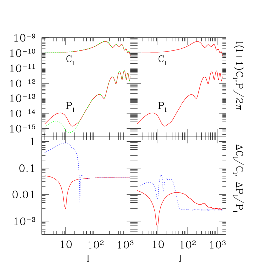
Figure 2: Top left: temperature ($C_{\ell}$) and polarization ($P_{\ell}$) angular power spectra versus the multipole $\ell$ for run A (solid line) and for prompt reionization (dotted line) when CMBFAST is run with $z_{i}=10.9$. Bottom left: the normalized temperature and polarization discrepancy as a function of angular multipole $\ell$ for this case. Here the solid and dotted lines refer to $C_{\ell}$ and $P_{\ell}$ respectively. Top right: temperature ($C_{\ell}$) and polarization ($P_{\ell}$) angular power spectra versus the multipole $\ell$ for run A (solid line) and for prompt reionization (dotted line) when CMBFAST is run with $\tau=0.08$. Bottom right: the normalized temperature and polarization discrepancy as a function of angular multipole $\ell$ for this case. Here the solid and dotted lines refer to $C_{\ell}$ and $P_{\ell}$ respectively.

3.3 Quantification of Errors & Tests of Our Approach

In order to quantify the difference between the fiducial model and the prompt model with the same optical depth further, we plot in Fig. 3 the quantity

$$\chi^{2}(\ell_{max})=\sum_{2}^{\ell_{max}}\frac{(2\ell+1)}{2}(\frac{\Delta C_{\ell}}{C_{\ell}})^{2}f_{sky}$$ (2)

as a function of the multipole number $\ell_{max}$ assuming full sky coverage, $f_{sky}=1$. For multipole values greater than 100, $\chi^{2}$ exceeds unity, the value corresponding to the cosmic variance error of $2C_{\ell}^{2}/(2\ell+1)$. This means that one can find a statistically significant difference between the prompt and fiducial models only by looking at angular multipoles with $\ell\lower 2.15277pt\hbox{$\;\buildrel>\over{\sim}\;$}100.$ However, in Fig. 2 we saw that the largest differences between the two histories occur at lower multipole values ($\ell=20-40$). Thus although these reionization histories are considerably different, it is almost impossible to discriminate between them observationally.

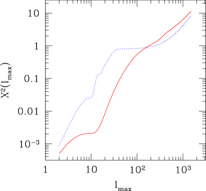
Figure 3: $\chi^{2}$ of $C_{\ell}$ (solid line) and of $P_{\ell}$ (dotted line) versus $\ell_{\rm max}$ (see eq. 2).

Finally, we extend our analysis to the runs B, C, and D of CFGJ, comparing them with prompt runs with equal values of $\tau_{s}$. These results are summarized in Table 1. As in run A, the values of $z_{i,p}$ found for these models correspond to times at which $x_{e,s}\approx 0.5$, when the IGM was in the midst of changing from a neutral state to an ionized one.

Is is clear from this table that it is not possible to put a constraint on the reionization redshift directly from CMBFAST. In fact, as can be easily seen in Table 1, the differences between $z_{i,s}$ and $z_{i,p}$ cannot be easily parameterized because they depend on several effects that influence the duration $\Delta z_{s}$ of the reionization process. These effects include radiative and stellar feedbacks, the star formation efficiency, the photon escape fraction, the spatial and mass distribution of the ionizing sources, and even the clumpiness of IGM, which is beyond the scope of the CFGJ simulations.

We have conducted a number of checks and convergence tests to assess the robustness of our approach. Our first check was to examine the overall, numerical value of the optical depth, which differs slightly from the input value due to the finite integration time step. Here we found that the output $\tau$s differ by less than $5\times 10^{-5}$ from the specified values. This corresponds to $\Delta C_{\ell}/C_{\ell}\lower 2.15277pt\hbox{$\;\buildrel<\over{\sim}\;$}10^{-4}$, i.e. $30$ times smaller than the actual difference between the simulated and prompt runs.

Next, we carried out a series of convergence tests, to ascertain the effects of $k$-mode sampling on our results. Here we restrict our tests to run A for which we increased the $k$ resolution by $50\%.$ A comparison between the original and resampled simulated runs showed that at most angular scales $\Delta C_{\ell}/C_{\ell}$ and $\Delta P_{\ell}/P_{\ell}$ are within $0.1\%$; larger differences (up to $\sim 0.7\%$) are found at higher multipole numbers ($\ell\lower 2.15277pt\hbox{$\;\buildrel>\over{\sim}\;$}700$). Comparing the resampled run A with a resampled prompt run with equal input optical depth, we found $\Delta C_{\ell}/C_{\ell}$ and $\Delta P_{\ell}/P_{\ell}$ values that were virtually indistinguishable from those obtained with low $k$ resolution runs.

Finally, we examined the effect of time sampling at both $k$ resolutions, comparing two prompt runs with equal optical depth and $k$ resolution, but forcing one of them to the same time step as in simulated run A. Again, we found $\Delta C_{\ell}/C_{\ell}$ and $\Delta P_{\ell}/P_{\ell}$ $\lower 2.15277pt\hbox{$\;\buildrel<\over{\sim}\;$}10^{-4}$, far smaller than the discrepancies between the prompt and simulated runs.

4 Conclusions

One of the first stages of nonlinear structure formation, reionization marked an important transition from a dark and relatively simple universe to one filled with a dazzling array of stars, galaxies, quasars, and other nonlinear objects. And although one of our best probes of this transition is through the measurement of CMB fluctuations, the process of reionization itself is much more dependent on the complicated astrophysical issues important at low redshifts than the linear issues important at $z\approx 1100.$

In this work, we have explored this transition, quantifying the impact of realistic scenarios of reionization on the angular power spectrum of the Comic Microwave Background. While standard estimates assume prompt reionization, we have considered instead a range of simulated models, each with a prolonged reionization epoch. We find that equating the redshift of full IGM ionization between these simulations and models that assume instantaneous reionization leads to widely discrepant temperature and polarization spectra. On the other hand, equating prompt and extended models with the same overall optical depth leads to differences in anisotropies that are nearly undetectable. In this case the redshift of complete ionization is lost in the complicated details of the phase transition, and comparisons yield $z_{i}$ values corresponding to roughly the point of 50% ionization in the simulations, although even this value is model dependent. It is clear then that while $z_{i}$ is useful as schematic tool, it is the total optical depth that is most accurate in providing a definition of the reionization epoch.

MB thanks M. Zaldarriaga for discussions and hospitality at IAS, Princeton where part of this work has been carried out. ES has been supported in part by an NSF MPS-DRF fellowship.

Table 1: Reionization parameters

Run	$\Delta z_{s}$(a)	$z_{i,s}$(b)	$\tau_{s}$(c)	$z_{i,p}$(d)	$x_{e,s}(z_{i,p})$(e)	$\frac{\Delta C_{\ell}}{C_{\ell}}$	$\frac{\Delta P_{\ell}}{P_{\ell}}$
$A$	15	$10.9$	0.080	17.1	0.46	$\lower 2.15277pt\hbox{$\;\buildrel<\over{\sim}\;$}0.01$	$\lower 2.15277pt\hbox{$\;\buildrel<\over{\sim}\;$}0.06$
$B$	17	$8.3$	0.059	13.9	0.51	$\lower 2.15277pt\hbox{$\;\buildrel<\over{\sim}\;$}0.007$	$\lower 2.15277pt\hbox{$\;\buildrel<\over{\sim}\;$}0.1$
$C$	15	$15$	0.098	19.8	0.48	$\lower 2.15277pt\hbox{$\;\buildrel<\over{\sim}\;$}0.01$	$\lower 2.15277pt\hbox{$\;\buildrel<\over{\sim}\;$}0.1$
$D$	17	$8.3$	0.064	14.7	0.47	$\lower 2.15277pt\hbox{$\;\buildrel<\over{\sim}\;$}0.008$	$\lower 2.15277pt\hbox{$\;\buildrel<\over{\sim}\;$}0.1$

Table 1: ^(a)Duration of reionization; ^(b)Redshift of complete reionization (simulated); ^(c)Thomson Optical Depth (simulated); ^(d)Redshift of complete reionization (prompt); ^(e)Hydrogen ionization fraction at $z_{i,p}$ (simulated).

References

- [1] Ciardi, B., Ferrara, A. & Abel, T. 2000, ApJ, 533, 594
- [2] Ciardi, B., Ferrara, A., Governato, F. & Jenkins, A. 2000, MNRAS, 314, 611 (CFGJ)
- [3] Barkana, R. & Loeb, A. 1999, ApJ, 523, 54
- [4] Becker, R. H. et al. 2001, astro-ph/0108097
- [5] De Bernardis, P. et al. 2000, Nature, 404, 955
- [6] De Bernardis, P., Balbi, A., De Gasperis, G., Melchiorri, A. & Vittorio, N. 1997, ApJ, 480, 1
- [7] Fabbri, R., 1999, New Astronomy Reviews, 43, 215
- [8] Gnedin, N.Y., 2001, astro-ph/0110290
- [9] Griffiths, L. M. & Liddle, A. R. 2001, MNRAS, 324, 769
- [10] Griffiths, L.M., Barbosa, D. & Liddle, A.R. 1999, MNRAS, 308, 854
- [11] Hanany, S. et al. 2000, ApJ, 545, L5
- [12] Hu, W. 2000, ApJ, 529, 12
- [13] Hu, W., Scott, D., Sugiyama, N. & White, M. 1995, Phys. Rev. D, 52, 5498
- [14] Naselsky, P. et al. 2001, astro-ph/0102378
- [15] Padin, S. et al. 2001, ApJ, 549, L1
- [16] Peebles, P.J.E. 1993, Principles of Physical Cosmology, Princeton, Princeton University Press
- [17] Tegmark, M., Zaldarriaga, M. & Hamilton, A.J.S. 2001, Phys. Rev. D, 43007
- [18] Tegmark, M. & Zaldarriaga, M. 2000, ApJ, 544, 30
- [19] Theuns, T., Zaroubi, S. & Kim, T.S. 2001, astro-ph/0110552
- [20] Schmalzing, J., Sommer-Larsen, J. & Goetz, M. 2000, astro-ph/0010063
- [21] Seljak, U. & Zaldarriaga, M. 1996, ApJ, 469, 437
- [22] Steidel, C.C. et al. 1999, ApJ, 519, 1
-
[23]
Zaldarriaga, M., 1997, Phys. Rev. D, 55, 1822