A SAURON study of M32: measuring the intrinsic flattening and the central black hole mass

Abstract

We present dynamical models of the nearby compact elliptical galaxy M32, using high quality kinematical measurements, obtained with the integral-field spectrograph SAURON mounted on the William Herschel Telescope on La Palma. We also include STIS data obtained by Joseph et al. We find a best-fit black hole mass of $M_{\bullet}=(2.5\pm 0.5)\times 10^{6}M_{\odot}$ and a stellar $I$-band mass-to-light ratio of $(1.85\pm 0.15)\,M_{\odot}/L_{\odot}$. For the first time, we are also able to constrain the inclination along which M32 is observed to $70^{\circ}\pm 5^{\circ}$. Assuming that M32 is indeed axisymmetric, the averaged observed flattening of 0.73 then corresponds to an intrinsic flattening of $0.68\pm 0.03$.

These tight constraints are mainly caused by the use of integral-field data. We show this quantitatively by comparing with models that are constrained by multiple slits only. We show the phase-space distribution and intrinsic velocity structure of the best-fit model and investigate the effect of regularisation on the orbit distribution.

1 Introduction

M32 is a high-surface brightness, compact E3 companion of the Andromeda galaxy. Ground-based kinematic measurements of this galaxy (Tonry 1984, 1987) already showed a steep gradient in the central velocity profile and a central dispersion peak, suggesting the presence of a central compact object, presumably a supermassive black hole. Since then, (spectroscopic) observations with increasing spatial resolution, both ground-based (Dressler & Richstone 1988; van der Marel et al. 1994a; Bender, Kormendy & Dehnen 1996) and with HST (Lauer et al. 1992; van der Marel, de Zeeuw & Rix 1997; Joseph et al. 2001), strengthened the case for this black hole.

Simultaneously, dynamical models of ever improving quality were built to match these data sets (Richstone, Bower & Dressler 1990; van der Marel et al. 1994b; Qian et al. 1995; Dehnen 1995). For most galaxies, the value of the best-fit black hole mass that is found depends on the assumptions that are made about the distribution function (DF) of the galaxy. Two-integral models, which assume that the DF depends only on the two classical integrals of motion (the energy $E$ and the vertical component of the angular momentum $L_{z}$), generally tend to overpredict the central black hole mass, since they cannot provide sufficient radial motion (Magorrian et al. 1998; Gebhardt et al. 2000; Bower et al. 2001).

The current state-of-the art models allow for the maximal degree of anisotropy by assuming that the distribution function depends on three integrals of motion (van der Marel et al. 1998, hereafter vdM98; Cretton et al. 1999, hereafter C99; Gebhardt et al. 2000, 2001). The internal kinematical structure of the best-fitting three-integral model of M32 closely resembles that of an $f(E,L_{z})$ model. This explains why the central black hole mass that was found in M32 by the early models does not differ much from the current value of $(3.4\pm 0.7)\times 10^{6}M_{\odot}$ (vdM98).

This means that the mass of the central black hole and intrinsic kinematical structure of M32 are constrained rather well. The main uncertainty that remains is the inclination along which M32 is observed, or, equivalently, the intrinsic flattening: edge-on models to a data-set consisting of FOS kinematics and ground-based observations along four position angles fit equally well as models that are projected over $55^{\circ}$ (vdM98). When we combine this with the observed flattening of M32 (which is almost constant and equal to $0.73$ inside the central ten arcseconds, vdM98), we see that the intrinsic flattening of M32 is not very tightly constrained and can have any value between $0.55$ and $0.73$.

Recent developments in instrument design offer a way out: integral-field spectrographs capture the full two-dimensional behaviour of objects and are therefore expected to better constrain parameters such as the inclination. This tighter constraint on the intrinsic parameters can be explained from the behaviour of two-integral models, even though these generally provide less accurate fits to observational data. The part of a two-integral distribution function that is even in the velocities is only determined once the meridional plane density distribution is known (Qian et al. 1995). The full intrinsic velocity map is needed to constrain the odd part of the DF, which means we need to measure the line-of-sight velocity $v_{\rm los}$. Whereas these two lowest order velocity moments are sufficient to determine the stellar DF of a galaxy, the dark matter distribution is only constrained once the velocity anisotropy is known (Dejonghe 1987; Gerhard 1991, 1993). This quantity can be measured through the higher order velocity moments. It is therefore necessary to determine the full two-dimensional kinematic behaviour of a galaxy. Capturing this information with only a few slit positions, as is generally attempted, is sometimes possible, but not always, which implies that the distribution function remains unconstrained.

These effects are even more important for three-integral distribution functions, which, in most cases, provide better fits to the observations and have more freedom. Therefore, when galaxy models are constrained by kinematic observations along a modest number of slits, the intrinsic structure may remain largely unconstrained. In this paper, we revisit M32 using two-dimensional kinematical maps obtained with the panoramic integral-field spectrograph SAURON (Bacon et al. 2001, hereafter Paper I; de Zeeuw et al. 2002, hereafter Paper II) and high-resolution spectra obtained with STIS on board HST (Joseph et al. 2001). We show that the use of integral-field data places very tight constraints on the central black hole mass and mass-to-light ratio of M32, but also, for the first time, on the inclination, or equivalently, the intrinsic flattening.

The paper is organized as follows: in Section 2, we give a brief summary of the data that are used to constrain the dynamical models, which are described in Section 3. The results are presented in Section 4 and we show in Section 5 that the use of integral-field data is crucial for most of the results that we obtained. The properties of the best-fitting model are described in Section 6, and we conclude with a discussion in Section 7.

Throughout the paper we assume a distance of $D=0.7$ Mpc (Welch et al. 1986). This choice does not influence our conclusions, but sets the scale of the models in physical units. Specifically, lengths and masses scale as $D$, while mass-to-light ratios scale as $D^{-1}$.

2 Observations

We use two fully complementary data sets obtained with current state-of-the-art instruments: the integral-field spectrograph SAURON mounted on WHT, and STIS on board HST. Integral-field spectrographs provide the full kinematic picture in one consistent data-set, while the high-resolution instrument STIS is ideal to probe the central kinematics of nearby objects. With this combined data-set, we expect to be able to determine the intrinsic properties of M32 with great accuracy.

2.1 SAURON observations

SAURON is mounted on the WHT on La Palma and is specifically designed to measure the kinematics and line-strengths of nearby ellipticals, lenticulars and spiral bulges. Details on the instrument and the data reduction process can be found in Paper I. The instrument has two observing modes: in the low-resolution mode, the field of view is $30\times 41$ arcsec at a pixel size of $0\aas@@fstack{\prime\prime}94$, while the high-resolution mode, used to zoom in on objects in good seeing conditions, has a pixel size of $0\aas@@fstack{\prime\prime}28$, corresponding to a field-of-view of $9\times 11$ arcsec.

The SAURON observations were made on October 15, 1999 (Paper II). Relatively good seeing (FWHM$\approx 0\aas@@fstack{\prime\prime}95$) allowed us to obtain the measurements in the high-resolution mode. The kinematical maps of M32, derived from a single 2700s exposure, are shown in the four upper panels of Fig. 1. The velocity field reaches a peak value of $\approx$ 65 km s^-1; the misalignment between the rotation axis and the projected minor axis is less than two degrees, demonstrating that the measurements are consistent with axisymmetry. The dispersion of M32 drops well below the instrumental resolution ($\sigma\approx$ 90 km s^-1) outside the inner few arcseconds. This results in a fourth-order Gauss-Hermite moment $h_{4}$ (measuring the symmetric deviations from a Gaussian, van der Marel & Franx 1993) that is difficult to measure. As is apparent from the fourth panel of Fig. 1, it is almost constant over the field.

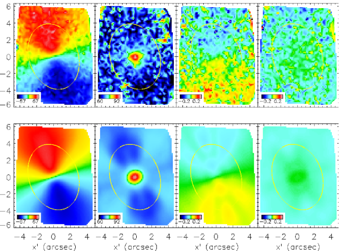
Figure 1: Top. The kinematic maps of M32 (from left to right: the mean velocity, velocity dispersion and Gauss-Hermite moments $h_{3}$ and $h_{4}$), as observed with the integral-field spectrograph SAURON. The field of view is $9\times 11$ arcsec. Bottom. The best fit kinematic maps, obtained by adding the weighted contributions of the best fitting set of orbits in the SAURON apertures.

A comparison of the SAURON measurements with ground-based long-slit data, obtained with the ISIS spectrograph on WHT, shows that the velocities differ only by $2.3\pm 2.2$ km s^-1, the dispersions by $6.0\pm 2.6$ km s^-1 and $h_{3}$ by $-0.009\pm 0.016$ (Paper II; the accuracy of $h_{4}$ is difficult to determine). This indicates that there is no systematic offset in $V$ and $h_{3}$, while the disagreement between the dispersion measurements is only significant at the 2$\sigma$-level. We do not correct for this and use all SAURON measurements to constrain the models.

2.2 STIS observations

The STIS measurements (Fig. 2) were obtained by Joseph et al. (2001), using the FCQ-method (Bender 1990). They clearly show the main signatures of a central black hole: a steep velocity gradient and a peak in the dispersion profile near the center. By assuming that M32 has a two-integral distribution function and by solving the Jeans equations, Joseph et al. estimate that a central black hole with a mass of $(2-4)\times 10^{6}M_{\odot}$ best reproduces these signatures, in full harmony with the earlier results by vdM98. STIS provides a continuous spatial sampling at $\approx 0\aas@@fstack{\prime\prime}051$ pixels, avoiding positioning problems that may occur when using aperture spectrographs such as FOS (van der Marel, de Zeeuw & Rix 1997). Comparisons between these two types of data are therefore only possible if such uncertainties are taken into account (Joseph et al. 2001). The STIS measurements are superior to the FOS data, since the spectral resolution and signal-to-noise ratio are much higher, an advantage when measuring the relatively low velocity and dispersion of M32. Because of this, we can use up to the fourth order Gauss-Hermite moment, while FOS was only able to measure the first two.

Figure 2: The panels show the major axis velocity, dispersion, third and fourth order Gauss-Hermite moments of M32 obtained with the high-resolution spectrograph STIS on board HST (diamonds, Joseph et al. 2001), together with the predictions at the STIS apertures of our best-fit model (solid line).

3 Method

3.1 Mass models

We construct dynamical models, based on Schwarzschild’s orbit superposition method (Schwarzschild 1979; 1982). We assume that the galaxy is axisymmetric and allow for the full degree of anisotropy by assuming that the distribution function depends on three integrals of motion. The implementation that is used here was originally developed by Rix et al. (1997), vdM98 and C99, and was designed for use on one-dimensional surface-brightness profiles (but see Cretton & van den Bosch 1999). However, for M32, as for most nearby ellipticals, high-quality two-dimensional imaging is available, so that more sophisticated density parametrisations are possible. An example of such a formalism is Multi-Gaussian Expansion (MGE, Monnet, Bacon & Emsellem 1992; Emsellem, Monnet & Bacon 1994), in which the set of Gaussians that best fits an image of the galaxy is found. The advantages of this formalism are that both axisymmetric and triaxial galaxies can be reproduced in a straightforward manner, the deprojection is simple and can be done analytically (under certain assumptions) once the viewing angles are known, and convolution with (MGE) point spread functions is fast and simple. We have therefore adapted the axisymmetric Schwarzschild software to use MGE; the new algorithm was tested while modeling the dynamics of the counter-rotating core galaxy IC1459 (Cappellari et al. 2002). These tests have shown that the modeling results do not depend on the choice of mass model: the best-fitting parameters and intrinsic (phase space) structure of models that start from an MGE parameterisation with constant axial ratio are identical to those of models that use a power-law density profile.

An MGE parameterisation of M32 was obtained using the software of Cappellari (2002), by fitting to a combination of a high-resolution HST/WFPC2/F814W image and a ground-based $I$-band image obtained by Peletier (1993; $0\aas@@fstack{\prime\prime}549$ pixels^-1 with a seeing of $1\aas@@fstack{\prime\prime}27$) with the Isaac Newton Telescope on La Palma. Since we are constructing axisymmetric models, we do not allow for shifts in the position angles of the Gaussians and fix the centers of all individual Gaussians to the center of the galaxy. Each Gaussian therefore has three free parameters: the amplitude $P^{\prime}$ (in units of $L_{\odot}\,{\rm pc}^{-2}$), the width $\sigma^{\prime}$ in pixels (or arcseconds) and the projected flattening $q^{\prime}$. Eleven Gaussians were used in the fit, since, upon adding more Gaussians, the RMS error of the fit does not change by more than 1%. The parameters of these eleven Gaussians are listed in Table 1; this superposition reproduces the M32 surface brightness with an RMS error of $\approx$2.2 per cent (Cappellari 2002, Figure 6). This is within the measurement errors.

Table 1: The parameters of the eleven Gaussians in the MGE-fit to the combined ground-based and HST/WFPC2/F814W image of M32. The second column shows the amplitude $P^{\prime}$, the third column shows the width $\sigma$ and the fourth the projected flattening of each Gaussian.

number	$P^{\prime}(L_{\odot}\,{\rm pc}^{-2})$	$\sigma^{\prime}$ (arcsec)	$q^{\prime}$
1	615412.	0.0364	0.740
2	517371.	0.131	0.809
3	324569.	0.348	0.775
4	175920.	0.753	0.732
5	54346	1.51	0.742
6	22279	3.18	0.708
7	11428	6.05	0.746
8	4037.5	11.7	0.683
9	2506.2	19.2	0.819
10	1142.4	33.5	0.820
11	226.4	95.8	0.827

3.2 Axisymmetric three-integral Schwarzschild models

We use the MGE-parameterisation to calculate axisymmetric three-integral models with the modified Schwarzschild method. Our models are different from those of previous authors: we use independent kinematic data sets and we parameterise the mass density differently. These differences provide a useful test: if we find best-fitting parameters that match the ones found by e.g. vdM98, it means that both approaches are reliable and the results are robust.

The set of best-fitting Gaussians is deprojected by assuming that the galaxy is axisymmetric and choosing a value of the inclination. The resulting intrinsic luminosity density is multiplied by a constant mass-to-light ratio $M/L$ to obtain the intrinsic mass density. The stellar potential can then be calculated by applying Poisson’s equation. A central supermassive black hole is mimicked by adding the potential of a central point mass $M_{\bullet}$. In the combined stellar and black hole potential, a representative orbit library is found by sampling the two classical integrals of motion, the energy $E$ and the vertical component of the angular momentum $L_{z}$, together with the third integral $I_{3}$.

Here, we only give a brief outline of the scheme that is used to sample these integrals; a more thorough description can be found in C99. The orbital energy is sampled through a logarithmic grid in the radius $R_{c}$ of the circular orbit at energy $E$. This grid is chosen to include more than $99.99$ per cent of the mass. While some of the orbits that make up the missing mass might contribute to the density in our radial range, this contribution will be smaller than $0.01$ per cent and can therefore be safely ignored.

At each energy, $L_{z}$ is sampled by a linear grid in the fractional angular momentum $L_{z}/L_{\rm max}\in\langle-1,1\rangle$, with $L_{\rm max}$ the maximum orbital angular momentum at energy $E$. This grid does not include $L_{z}/L_{\rm max}=\{0,1\}$ to avoid problems with the numerical integration. This is not a severe limitation, as the orbits that are missed in this manner carry only a small fraction of the mass in an axisymmetric model. The third integral is parameterised by the orbital starting point on the zero velocity curve.

Every combination of the integrals $(E,L_{z},I_{3})$ defines a separate stellar orbit. Since the third integral is generally not known analytically, the orbital properties can only be obtained by solving the equations of motion numerically. At every time step of this orbit integration, which is carried out for a fixed number of characteristic orbital periods (usually chosen to be the period of the circular orbit at the given energy), the orbital energy is randomized by drawing a number of arbitrary values from the energy bin around $E$, which are then assigned to the orbit. This ’dithering’ of integral space results in smoother orbital superpositions, which generally provide better fits to the data (Zhao 1996; C99).

The orbital superposition can be made even smoother by including the so-called two-integral components (TICs, C99; Verolme & de Zeeuw 2002) in the orbit library. These TICs are building blocks that obey only the two classical integrals of motion $E$ and $L_{z}$ and implicitly include stochastic orbits at the given values of energy and angular momentum. Since they are smoother than most orbits, the orbital superposition also suffers less from discretisation when they are included in the library. Here, we calculated model fits to different data-sets (both long-slit and integral-field data) with and without TICs in the orbit library, and found that the fit improves only marginally upon inclusion of the TICs (RMS error of the fit changes by less than 0.1%). On the other hand, calculating observables for the TICs at every aperture can be very time-consuming when many data points are included in the fit, as is the case when using integral-field data. To save computation time, we therefore decided not to include the TICs in the derivation of the best-fit parameters.

The observables of all orbits (and TICs) in the library are stored on grids that are adapted to the resolution of the observations. Using these, the orbital superposition that best fits the data is found by applying the non-negative least-squares (NNLS) routine of Lawson & Hanson (1974). The (unavoidable) discrepancy between model predictions and data, caused by noise in the data, discretisation effects and wrong choices of the model parameters, is expressed in a value for the $\chi^{2}$, defined as

$$\chi^{2}=\sum_{i=1}^{N_{d}}\left(\frac{D^{*}_{i}-D_{i}}{\Delta D_{i}}\right)^{2},$$ (1)

where $N_{d}$ is the number of constraint points, $D_{i}$ is the observational constraint at the $i$-th data point, $D^{*}_{i}$ is the model prediction at that point and $\Delta D_{i}$ is the uncertainty that is associated with this value (usually the observational error). By varying the inclination, central black hole mass and stellar mass-to-light ratio, we investigate which combination $(M_{\bullet},M/L,i)$ results in the overall smallest $\chi^{2}$ (the overall best fit to the data). The value of $\chi^{2}$ for a single model is of limited value, since the true number of degrees of freedom is generally not known, but the difference in $\chi^{2}$ between a model and the overall minimum value, $\Delta\chi^{2}=\chi^{2}-\chi^{2}_{\rm min}$, is statistically meaningful (see Press et al. 1992). By using the central limit theorem, it can be shown that this interpretation is even valid when the errors $\Delta D_{i}$ are not Gaussian distributed (van der Marel et al. 2000), which is important when applying the statistic to models of observational data. This means that we can assign the usual confidence levels to the $\Delta\chi^{2}$ distribution and determine the probability that a given set of model parameters will occur.

Introducing integral-field data in numerical models also means a considerable increase in the number of measurements that has to be reproduced: even when only one SAURON pointing is used, a fit to both the intrinsic and projected mass density and to all four Gauss-Hermite moments results in approximately 8000 constraints. Standard mathematical practice in minimization problems is to use more free parameters than constraints, which means we would need $\sim 10^{4}$ orbits to fit a SAURON field. On the other hand, the behaviour of models that are only constrained by observational data is very similar to that of models with additional regularisation constraints (R97; C99; vdM98; Fig. 5 of this paper), even though regularised models always have more constraints than orbits (§4.2).

We conclude from this that it is not necessary to use more orbits than constraints to obtain accurate and unbiased fits to the data. In our case, we decided to use an orbit library with $N_{o}=20\times 7\times 7$ orbits. Since the orbital $L_{z}$ can be both positive or negative, depending on the chosen direction of rotation around the symmetry axis, this results in a library of 1960 orbits, implying that we have almost four constraints per orbit.

When using integral-field data, the integration time of individual orbits may become extremely lengthy, as their properties have to be stored in many apertures. This is another reason not to use very large orbit libraries. Integrating all orbits in our library requires about eight hours of computation time on a 1GHz machine with 512Mb memory, while one NNLS fit takes approximately one hour on the same machine.

4 Results

4.1 Best-fit intrinsic parameters

We sample the model parameters $(M_{\bullet},M/L,i)$ on a grid of 990 models, defined by fifteen values of the central black hole mass, spaced linearly between $M_{\bullet}=0$ and $M_{\bullet}=4.5\times 10^{6}M_{\odot}$, eleven values of $M/L$ between 1.5 and 2.5, and inclinations $i=90^{\circ},75^{\circ},70^{\circ},65^{\circ},60^{\circ}$ and $50^{\circ}$. We do not consider smaller values of the inclination, as this would make M32 intrinsically flatter than E7, i.e., flatter than any observed elliptical galaxy. Models with equal ratios between the mass-to-light ratio and the central black hole mass differ only by a scaling factor in the velocity. This means that, for every inclination, only fifteen orbit libraries have to be calculated, each with a different ratio $M_{\bullet}/(M/L)$. Any point along a line of constant $M_{\bullet}/(M/L)$ can then be obtained by scaling the velocity prior to the NNLS fit. As a result, one full $\chi^{2}(M_{\bullet},M/L)$ grid (at fixed inclination) takes about twelve days of computation time.

For each of the 990 models that were obtained in this manner, we calculated the fit to the combined SAURON and STIS data. Contour plots of the values of $\chi^{2}(M_{\bullet},M/L,i)$, offset such that the overall minimum value is zero, are shown in Fig. 3.

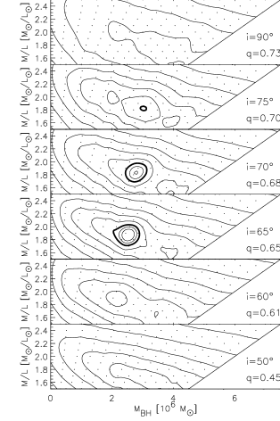
Figure 3: $\Delta\chi^{2}$ as a function of central black hole mass $M_{\bullet}$, stellar mass-to-light ratio $M/L$ and inclination $i$. The inclination varies from $90^{\circ}$ (top panel) to $50^{\circ}$ (bottom panel), and $\chi^{2}$ is offset such that the overall minimum is zero. Contours are drawn at the formal confidence levels for a $\Delta\chi^{2}$-distribution with three degrees of freedom, with the inner three contours corresponding to the 1$\sigma$, 2$\sigma$ and 3$\sigma$ confidence levels (the thick contour indicates the 3$\sigma$ level); subsequent contours correspond to a factor of two increase in $\Delta\chi^{2}$.

The contour levels correspond to the confidence levels of a $\Delta\chi^{2}$ distribution with three degrees of freedom (with the thick contour in the figure indicating the 3$\sigma$ confidence level), so that the volume in which the intrinsic parameters of M32 are most likely located can be readily assessed. The shape of the contours is very regular, even though no smoothing has been applied.

The best-fitting edge-on model has a black hole mass of $(4.0\pm 0.5)\times 10^{6}M_{\odot}$ (3$\sigma$-error), which agrees very well with the vdM98’s value of $(3.4\pm 0.7)\times 10^{6}M_{\odot}$, even though the observational data sets are independent. However, we see from Fig. 3 that models with an inclination in the range $i=70^{\circ}\pm 5^{\circ}$ provide significantly better fits to the data than models with other inclinations, which are ruled out at high confidence. This narrow constraint on the inclination corresponds to an intrinsic flattening of approximately $0.68\pm 0.03$ (given the observed flattening of 0.73).

The overall best-fit model, located at $i=70^{\circ}$, has a black hole mass of $(2.5\pm 0.5)\times 10^{6}M_{\odot}$ and an $I$-band mass-to-light ratio of $(1.85\pm 0.15)\,M_{\odot}/L_{\odot}$. The fit of this model to the SAURON data is shown in the bottom panels of Fig. 1; the fit to the STIS data is given in Fig. 2.

4.2 Applying regularisation

The matrix problem that is solved by the NNLS routine is often ill-conditioned, resulting in orbital weights $\gamma(E,L_{z},I_{3})$ that vary rapidly as a function of the integrals of motion. This can be avoided by imposing regularisation constraints on the orbital weights (see e.g. Press et al. 1992; Merritt 1993; Zhao 1996; Rix et al. 1997); another method, with similar effect, is to add maximum entropy constraints (Richstone & Tremaine 1988). Applying regularisation forces the orbital weights towards a smooth function of $E,L_{z}$ and $I_{3}$ by minimizing the $n$-th order derivatives $\partial^{n}\gamma(E,L_{z},I_{3})/\partial E^{n},\partial^{n}\gamma(E,L_{z},I_{3})/\partial L^{n}_{z}$ and $\partial^{n}\gamma(E,L_{z},I_{3})/\partial I^{n}_{3}$. The degree of smoothing is determined by the order $n$ and by the maximum fractional error $\Delta$ that the derivatives are allowed to have. For all regularised models that are described here, we have minimized the second-order derivative ($n=2$).

The optimal value of the regularisation error $\Delta$ was determined by calculating model fits for a fixed combination of ($M_{\bullet},M/L,i$) and varying $\Delta$ between $0.1$ (high regularisation) and $\infty$ (no regularisation). Fig. 4 shows that $\chi^{2}$ is large for small values of $\Delta$, but quickly decreases to an almost constant level for $\Delta>4$.

Figure 4: $\chi^{2}$ as a function of the regularisation parameter, at fixed $M_{\bullet}$, $M/L$ and inclination. The model with no regularisation is located at $\Delta=\infty$, but is placed at $\Delta=500$ to include the value in the plot.

Since the ideal model both fits the constraints and has a smooth distribution of orbital weights, we use $\Delta=4$ whenever regularisation is needed. A similar degree of smoothing was used earlier in applications that use the same regularisation technique (vdM98; Cretton & van den Bosch 1999) and in models that use the maximum entropy method (Gebhardt et al. 2000).

Including smoothing constraints in the NNLS fit will, in general, change the value of $\chi^{2}$ and therefore may affect the shape of the contours in plots such as Fig. 3. The top panel of Fig. 5 shows a cross-section of Fig. 3 at $M/L=1.8$; the $\chi^{2}$ of fits with the same parameters, but including regularisation, is shown in the middle panel. Since the shape of the contours does not change significantly, applying regularisation does not change the overall best-fit parameters, while it allows us to better study the phase-space structure and internal motions (see Fig. 7 below).

The two upper panels were calculated using four constraints per orbit ($N_{d}/N_{o}=4$, the value that is used throughout the paper). Although we already argued in § 3.2 that our results are not sensitive to this parameter, we investigated this more quantitatively by calculating (unregularised) models for which $N_{d}/N_{o}=0.6$, which means there are almost two orbits per constraint point. The result of this is shown in the bottom panel, which indeed illustrates that our results do not depend on the number of orbits that is used.

Figure 5: $\Delta\chi^{2}$ as a function of central black hole mass and inclination, for a fixed $M/L$ of 1.8, for models without regularisation (top panel) and with regularisation (middle panel). The shape of the contours does not change upon adding regularisation. The bottom panel was calculated with $N_{d}/N_{o}=0.6$ and no regularisation, showing that our results do not depend on the number of orbits in the fit.

5 The effect of integral-field data

At this point, although we have shown that the model parameters are constrained much more tightly than in any previous model, it is not entirely clear to what extent this is caused by the use of integral-field data. We also have to take into account that we have used a very dense sampling of $M_{\bullet}$ and $M/L$, that we were able to calculate models at more inclinations than vdM98, and that the STIS data is of higher quality than the FOS observations. A more quantitative estimate of the influence of the integral-field data on the $\chi^{2}$ contours and on the best fitting parameters can be obtained by repeating the procedure of Section 3 for a data set that closely resembles the one used by vdM98. Since they fitted to a combination of FOS pointings with ground-based long-slit observations along the major, minor, $45^{\circ}$ and $135^{\circ}$ axes (which agree with SAURON), a similar data set can be obtained by extracting virtual ‘slits’ from the SAURON field along the same position angles and combining these with the STIS data.

Figure 6: Similar to Fig. 3, for model fits to a data set consisting of the STIS data and virtual ‘slits’ simulated from the SAURON data. The range of best-fitting values in all three model parameters is much larger than in Fig. 3, which indicates that using integral-field data tightens the constraint on all model parameters.

This data set was used to constrain models with the same parameter ranges as described in Section 3. Fig. 6 shows the $\chi^{2}$ of these fits. The best-fitting black hole mass is $M_{\bullet}=(2.8\pm 1.2)\times 10^{6}M_{\odot}$, the $I$-band mass-to-light ratio is $(1.75\pm 0.25)\,M_{\odot}/L_{\odot}$ and the inclination can have any value below $75^{\circ}$. A comparison with the best-fit parameters of Section 4 indicates that the volume of intrinsic parameters providing a reasonable fit to the data is significantly larger for the slit data set than when the entire SAURON field is used. We also notice that, although the use of integral-field data tightens the constraint on all model parameters (with a fractional change in the allowed range of $M_{\bullet}$ of 2.4 when changing from integral-field to slit data, and 1.7 for $M/L$), the most dramatic effect occurs for the inclination, which has an eight times larger allowed range when the galaxy is observed along a few slits only.

This can be explained from the behaviour of two-integral models, even though these generally provide less accurate fits to observational data. As was mentioned in the Introduction, in order to constrain the even part of a two-integral distribution function, one needs to specify the meridional plane density distribution (Qian et al. 1995). The odd part is determined once the full intrinsic velocity field is known, which can only be measured through the projected velocity field $v_{z^{\prime}}(x^{\prime},y^{\prime})$ (in which $x^{\prime}$ and $y^{\prime}$ are the coordinates in the plane of the sky). Furthermore, even if the total stellar DF is determined accurately, the dark matter distribution is still unconstrained. This can be solved by measuring the higher order velocity moments, which are related to the anisotropy of the velocity distribution.

When the projected velocity moments are simple functions of $x^{\prime}$ and $y^{\prime}$, measurements at a small number of positions are sufficient to determine the behaviour at all intermediate position angles. Indeed, some very specific two-integral models, such as the power-law galaxies (Evans & de Zeeuw 1994), have velocity fields that are quadratic in $x^{\prime}$ and $y^{\prime}$, implying that observations along two perpendicular slits are sufficient to determine their full two-dimensional kinematical behaviour.

However, most galaxies require a distribution function that depends on three integrals of motion. The velocity fields of these three-integral models (and, in fact, of most generally applicable two-integral models) are usually much more complicated functions of the projected coordinates (Dehnen & Gerhard 1993; de Bruijne, van der Marel & de Zeeuw 1996). This means that these velocity fields cannot be characterized by a (small) number of slit orientations. It is therefore not surprising that realistic models constrained by observations along only a few slit orientations cannot provide much information about the intrinsic shape of the galaxy. It also implies that integral-field data places constraints on the intrinsic shapes of galaxies, as well as on their mass distribution.

We see in both Fig. 3 and Fig. 6 that the best-fitting black hole mass of each separate panel increases with inclination. This behaviour can be understood at least partially from the following: the contribution of the intrinsic rotational velocity $v_{\phi}$ to the line-of-sight velocity decreases proportionally to $\sin i$. However, at smaller inclinations, the model must also be intrinsically flatter, which means $v_{\phi}$ is larger when lowering $i$. For a two-integral model, the increase in $v_{\phi}$ is dominant, so that there is more net velocity at smaller values of the inclination. This also implies that less mass is needed to obtain the same velocity field. Unfortunately, since there is a trade-off between the mass-to-light ratio and the central black hole mass and because we are dealing with three-integral models, it is not clear to what extent these considerations can explain the effect we observe.

6 Properties of the best-fit model

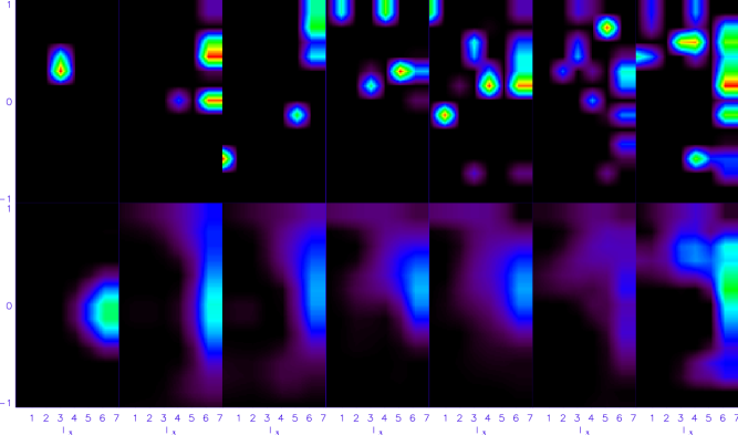
Figure 7: Best-fit model orbital weights as a function of the three integrals of motion $E,L_{z}$ and $I_{3}$. Each panel shows the orbital weights as a function of $I_{3}$ and $L_{z}$ (in units of the angular momentum of the circular orbit; since orbits can move in both the prograde and retrograde direction, $L_{z}/L_{\rm max}$ can be either positive or negative) at constant $E$. The energy decreases from left to right, corresponding to an increasing mean orbital radius (from $0\aas@@fstack{\prime\prime}01$ in the left panel to $\approx 10$ arcsec in the right panel. Larger radii are not shown, since these are not meaningfully constrained by the data). Top panels: the rapidly varying orbital weights for the unregularised model. Bottom panels: including a modest degree of regularisation ($\Delta=4$) smoothens the orbital weights, while still fitting the constraints. The color scheme is the same as in the upper panels.

The upper panels of Fig. 7 show the phase-space distribution of the orbits of the non-regularised best-fit model as a function of $I_{3}$ and $L_{z}$, for constant $E$. The energy decreases from left to right, corresponding to an increasing distance from the galaxy center. The bottom panels are similar, for the model with a regularisation error of $\Delta=4$.

We can study the intrinsic dynamical structure of the best-fitting model ($M_{\bullet}=2.5\times 10^{6}M_{\odot}$, $M/L$=1.85 $M_{\odot}/L_{\odot,I}$, $i=70^{\circ}$) by adding the appropriate moments of the orbits with non-zero weight. This implies that we can study the degree of anisotropy of the model, and from this determine to what extent the galaxy resembles a two-integral model. Fig. 8 shows the intrinsic velocity moments $\langle v^{2}_{r}\rangle^{\frac{1}{2}}$ (solid line), $\langle v^{2}_{\theta}\rangle^{\frac{1}{2}}$ (dotted line) and $\langle v^{2}_{\phi}\rangle^{\frac{1}{2}}$ (dashed line) of the best-fitting model, as a function of the meridional plane radius and the angle from the symmetry axis. The velocity moments are normalized by the total RMS motion $\langle v^{2}\rangle=\langle v^{2}_{r}\rangle+\langle v^{2}_{\theta}\rangle+\langle v^{2}_{\phi}\rangle$. We see that the model resembles an $f(E,L_{z})$ model near the equatorial plane ($\langle v^{2}_{r}\rangle^{\frac{1}{2}}=\langle v^{2}_{\theta}\rangle^{\frac{1}{2}}$) and becomes increasingly more anisotropic towards the symmetry axis. This indicates that a two-integral model is not suitable to fit all constraints simultaneously, in agreement with the findings of vdM98 (their Fig. 10). Furthermore, as in their models, azimuthal motion dominates.

Figure 8: Three intrinsic velocity moments $\langle v^{2}_{r}\rangle^{\frac{1}{2}}$ (solid line), $\langle v^{2}_{\theta}\rangle^{\frac{1}{2}}$ (dotted line) and $\langle v^{2}_{\phi}\rangle^{\frac{1}{2}}$ (dashed line) as a function of the meridional plane radius and the angle from the symmetry axis, for the best-fitting model without regularisation. The velocity moments are normalized by the total RMS motion, $\langle v^{2}\rangle$.

For completeness, we have checked the internal kinematical structure of the pseudo-slit model for the same parameters as were used for Fig. 8. Since this combination of intrinsic parameters is inside the 3$\sigma$ contour of Fig. 6, and therefore also provides a good fit to the data, the results resemble those of Fig. 8 closely. The main difference between using slits and integral-field data is that more combinations of intrinsic parameters can be ruled out by integral-field data. A point ($M_{\bullet},M/L,i$) that is not inside the 3$\sigma$ contour of Fig. 3, but cannot be ruled out by observations along a few slits, will therefore in general show a different intrinsic kinematical structure.

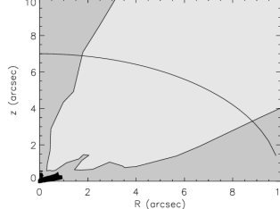
Figure 9: A greyscale plot of the anisotropy parameter $\beta_{B}$ as a function of the meridional plane coordinates $R$ and $z$, together with a typical isodensity contour (using $i=70^{\circ}$). The values were obtained by summing up the intrinsic moments of the set of orbits with non-zero weight in the best-fitting model. The darkest regions correspond to radial anisotropy ($\beta_{B}>0$); the lightest region shows the points where the model is tangentially anisotropic ($\beta_{B}<-1$). In all other points, the model is only mildly anisotropic ($-1<\beta_{B}<0$).

The anisotropy of a model can also be expressed in terms of an anisotropy parameter. A possible definition of this parameter is

$$\beta_{B}=1-\frac{\langle v^{2}_{\theta}\rangle^{\frac{1}{2}}+\langle v^{2}_{\phi}\rangle^{\frac{1}{2}}}{2\,\langle v^{2}_{r}\rangle^{\frac{1}{2}}}.$$ (2)

When the model is fully isotropic, $\beta_{B}=0$, while $\beta_{B}=1$ for a model that consists entirely of radial orbits, and $\beta_{B}=-\infty$ describes a model with only circular orbits. Fig. 9 shows this parameter as a function of the meridional plane coordinates $R$ and $z$, over the range that is constrained by the SAURON data. A typical isodensity contour is overplotted (using $i=70^{\circ}$). We see that $\beta_{B}$ is positive close to the galaxy center, so that the velocity distribution is radially anisotropic there. In all other parts of the meridional plane, the model is azimuthally anisotropic. This result does not change upon adding regularisation.

Dynamical models of elliptical galaxies have revealed that a few other objects are also tangentially anisotropic (NGC4697, Dejonghe et al. 1996; NGC1700, Statler et al. 1999), while the majority seems to be radially anisotropic (M87, Merritt & Oh 1997; NGC2324, R97; NGC6703, Gerhard et al. 1998; M32, vdM98; NGC1600, Matthias & Gerhard 1999; NGC3379, NGC3377, NGC4473, NGC5845, Gebhardt et al. 2000; NGC1399, Saglia et al. 2000). However, this radial anisotropy is usually rather small and sometimes even accompanied by a transition to isotropy at small radii. Furthermore, not all models included the full velocity profile in the fit, which implies that the mass-anisotropy degeneracy may not have been broken. Finally, our models are the first to use fully two-dimensional kinematical observations, which makes comparison with earlier models even harder. Therefore, although our results seem to contradict these findings, we must also conclude that our knowledge of anisotropy is still limited.

7 Conclusions

We have presented dynamical models of the nearby compact elliptical M32, using data from the integral-field spectrograph SAURON and from STIS on board HST. We have shown that our modeling software is able to deal with two-dimensional kinematical information and that the integral-field data tightens the constraint on all intrinsic model parameters considerably.

The axisymmetric three-integral model that best fits the data has a black hole mass of $(2.5\pm 0.5)\times 10^{6}M_{\odot}$ and a stellar $I$-band mass-to-light ratio of $(1.85\pm 0.15)\,M_{\odot}/L_{\odot}$. These values confirm the best-fit parameters that were obtained by previous authors, although our modeling procedure is different: we use a fully independent kinematical data-set and a different parameterisation for the mass density. Despite these differences in the methods, the best-fitting parameters that we find match the ones that were found by e.g. vdM98. This means that both approaches are reliable and that the results are robust.

For the first time, we are able to determine the inclination along which M32 is observed with great accuracy: the best-fit value is $70^{\circ}\pm 5^{\circ}$. If M32 is indeed axisymmetric, the averaged observed flattening of 0.73 then corresponds to an intrinsic flattening of $0.68\pm 0.03$. We have shown in Section 5 that this tight constraint is mainly caused by the use of integral-field data. This implies that integral-field data will provide us with more insight into the internal structure and kinematics of such objects.

Although M32 is consistent with axisymmetry, it may be intrinsically triaxial, but seen along one of its principal planes. Allowing for an intrinsically triaxial object also would enable us to study the effects of uncertainties in the deprojection on the best-fitting parameters more closely. An extension of our method to triaxiality is in progress (Verolme et al. 2002, in prep.), which will allow us to verify the assumptions made here. Furthermore, the tests that were carried out in this paper and the agreement with the results of other authors indicate that, given the assumptions, the results are robust.

We have obtained observations with SAURON of a representative sample of nearby ellipticals, lenticulars and spiral bulges, for most of which high-resolution STIS data is, or will become, available. We are in the process of applying the axisymmetric version of Schwarzschild’s method on SAURON observations of a few of the sample galaxies that appear consistent with axisymmetry (e.g. NGC821, NGC3377, NGC2974). The results of these dynamical models will provide us with the intrinsic parameters of a considerable number of objects, giving us unique insight into the formation and evolution of early-type galaxies.

Acknowledgements
We thank Karl Gebhardt, Richard McDermid and Glenn van de Ven for useful discussions, and Eric Emsellem, Harald Kuntschner and Reynier Peletier for a critical reading of the manuscript. YC acknowledges support through a European Community Marie Curie Fellowship. MB acknowledges support from NASA through Hubble Fellowship grant HST-HF-01136.01 awarded by the Space Telescope Science Institute, which is operated by the Association of Universities for Research in Astronomy, Inc., for NASA, under contract NAS 5-26555.

References

- [1] Bacon et al., 2001, MNRAS, 326, 23 (Paper I)
- [2] Bender R., 1990, A&A, 229, 441
- [3] Bender R., Kormendy J., Dehnen W., 1996, ApJ, 464, L123
- [4] Binney J.J., 1980, MNRAS, 190, 873
- [5] van den Bosch F.C., 1997, MNRAS, 287, 543
- [6] Bower G.A. et al., 2001, ApJ, 550, 75
- [7] de Bruijne J.H.J., van der Marel R.P., de Zeeuw P.T., 1996, MNRAS, 282, 909
- [8] Cappellari M., 2002, MNRAS, in press, astro-ph/0201430
- [9] Cappellari M., Verolme E.K., van der Marel R.P., Verdoes Kleijn G.A., Illingworth G.D., Franx M., Carollo C.M., de Zeeuw P.T., 2002, ApJ, submitted, astro-ph/0202155
- [10] Cretton N., de Zeeuw P.T., van der Marel R.P., Rix H.-W., 1999, ApJS, 124, 383 (C99)
- [11] Cretton N., van den Bosch F.C., 1999, ApJ, 514, 704
- [12] Davies R.L. et al., 2001, ApJ, 548, L33
- [13] Dehnen W., Gerhard O.E., 1993, MNRAS, 261, 311
- [14] Dehnen W., 1995, MNRAS, 274, 919
- [15] Dejonghe H.B., 1987, MNRAS, 224, 13
- [16] Dejonghe H., de Bruyne V., Vauterin P., Zeilinger W. W., 1996, A&A, 306, 363
- [17] Dressler A., Richstone D.O., 1988, ApJ, 324, 701
- [18] Emsellem E., Monnet G., Bacon R., 1994, A&A, 285, 723
- [19] Evans N.W., de Zeeuw P.T., 1994, MNRAS, 271, 202
- [20] Gebhardt K. et al., 2000, AJ, 119, 1157
- [21] Gebhardt K. et al., 2001, AJ, 122, 2469
- [22] Gerhard O.E., MNRAS, 1991, 250, 812
- [23] Gerhard O.E., MNRAS, 1993, 265, 213
- [24] Gerhard O. E., Jeske G., Saglia R. P., Bender R., 1998, MNRAS, 295, 197
- [25] Joseph C. et al., 2001, ApJ, 550, 668
- [26] Lauer T.R. et al., 1992, AJ, 104, 552
- [27] Lawson C.L., Hanson R.J., 1974, Solving Least Squares Problems (Englewood Cliffs: Prentice Hall)
- [28] Magorrian J. et al., 1998, AJ, 115, 2285
- [29] van der Marel R.P., Franx M., 1993, ApJ, 407, 525
- [30] van der Marel R.P., Rix H.-W., Carter D., Franx M., White S.D.M., de Zeeuw P.T., 1994a, MNRAS, 268, 521
- [31] van der Marel R.P., Evans N.W., Rix H.-W., White S.D.M., de Zeeuw P.T., 1994b, MNRAS, 271, 99
- [32] van der Marel R.P., de Zeeuw P.T., Rix H.-W., 1997, ApJ, 488, 119
- [33] van der Marel R.P., Cretton N., de Zeeuw P.T., Rix H.-W., 1998, ApJ, 493, 613 (vdM98)
- [34] van der Marel R.P. et al., 2000, AJ, 119, 2038
- [35] Matthias M., Gerhard O.E., 1999, MNRAS, 310, 879
- [36] Merritt D., 1993, ApJ, 413, 79
- [37] Merritt D., Oh S. P., 1997, AJ, 113, 1279
- [38] Monnet G., Bacon R., Emsellem E., 1992, A&A, 253, 366
- [39] Peletier R.F., 1993, A&A, 271, 51
- [40] Press W.H., Teukolsky S.A., Vettering W.T., Flannery B.P., 1992, Numerical Recipes (Cambridge: Cambridge Univ.Press)
- [41] Qian E.E., de Zeeuw P.T., van der Marel R.P., Hunter C., 1995, MNRAS, 274, 602
- [42] Richstone D., Tremaine S., 1988, ApJ, 327, 82
- [43] Richstone D., Bower G., Dressler A., 1990, ApJ, 353, 118
- [44] Rix H.-W., de Zeeuw P.T., Cretton N., van der Marel R.P., Carollo C.M., 1997, ApJ, 488, 702 (R97)
- [45] Saglia R. P., Kronawitter A., Gerhard O. E., Bender R., 2000, AJ, 119, 153
- [46] Schwarzschild M., 1979, ApJ, 232, 236
- [47] Schwarzschild M., 1982, ApJ, 263, 599
- [48] Statler T. S., Dejonghe H., Smecker-Hane T., 1999, AJ, 117, 126
- [49] Tonry J.L., 1984, ApJ, 283, L27
- [50] Tonry J.L., 1987, ApJ, 322, 632
- [51] Verolme E.K., de Zeeuw P.T., 2002, MNRAS, 331, 4
- [52] Welch D.L., Madore B.F., McAlary C.W., McLaren R.A., 1986, ApJ, 305, 583
- [53] de Zeeuw et al., 2002, MNRAS, 329, 513 (Paper II)
- [54] Zhao H.S., 1996, MNRAS, 283, 149