The time variation in infrared water-vapour bands in Mira variables

The time variation in the water-vapour bands in oxygen-rich Mira variables has been investigated using multi-epoch ISO/SWS spectra of four Mira variables in the 2.5–4.0 $\mu$m region. All four stars show H₂O bands in absorption around minimum in the visual light curve. At maximum, H₂O emission features appear in the $\sim$3.5–4.0 $\mu$m region, while the features at shorter wavelengths remain in absorption. These H₂O bands in the 2.5–4.0 $\mu$m region originate from the extended atmosphere.

The analysis has been carried out with a disk shape, slab geometry model. The observed H₂O bands are reproduced by two layers; a ‘hot’ layer with an excitation temperature of 2000 K and a ‘cool’ layer with an excitation temperature of 1000–1400 K. The column densities of the ‘hot’ layer are $6\times 10^{20}$–$3\times 10^{22}$ cm^-2, and exceed $3\times 10^{21}$ cm^-2 when the features are observed in emission. The radii of the ‘hot’ layer ($R_{\mathrm{hot}}$) are $\sim$1 $R_{*}$ at visual minimum and 2 $R_{*}$ at maximum, where $R_{*}$ is a radius of background source of the model, in practical, the radius of a 3000 K black body. The ‘cool’ layer has the column density ($N_{\mathrm{cool}}$) of $7\times 10^{20}$–$5\times 10^{22}$ cm^-2, and is located at 2.5–4.0 $R_{*}$. $N_{\mathrm{cool}}$ depends on the object rather than the variability phase.

The time variation of $\mbox{$R_{\mathrm{hot}}$}/R_{*}$ from 1 to 2 is attributed to the actual variation in the radius of the H₂O layer, since the variation in $R_{\mathrm{hot}}$ far exceeds the variation in the ‘continuum’ stellar radius. A high H₂O density shell occurs near the surface of the star around minimum, and moves out with the stellar pulsation. This shell gradually fades away after maximum, and a new high H₂O density shell is formed in the inner region again at the next minimum. Due to large optical depth of H₂O, the near-infrared variability is dominated by the H₂O layer, and the L’-band flux correlates with the area of the H₂O shell. The infrared molecular bands trace the structure of the extended atmosphere and impose appreciable effects on near-infrared light curve of Mira variables.

1 Introduction

Asymptotic Giant Branch (AGB) stars are in the late stage of the stellar evolution for low and intermediate main-sequence mass stars. Generally, AGB stars are pulsating variables as represented by Mira variables. According to hydrodynamic model atmospheres, the pulsations lift up matter from the stellar surface and extend the atmosphere (e.g. Bowen Bowen88 (1988)). Pulsations create shocks, causing a step-like structure in the density distribution as a function of radius (e.g. Fleischer et al. Fleischer92 (1992); Höfner et al. Hoefner98 (1998)). The cooling behind the shock is efficient (Woitke et al. Woitke96 (1996)) and the temperature decreases immediately in the post-shock regions (Fleischer et al. Fleischer92 (1992); Höfner et al. Hoefner98 (1998)).

The extended atmosphere is filled with various kinds of molecules. The structure of the extended atmosphere can be studied using infrared molecular bands. Hinkle (Hinkle78 (1978)) and Hinkle & Barnes (Hinkle79 (1979)) analyzed high resolution spectra of the oxygen-rich Mira, R~Leo, and found two velocity components in the near-infrared molecular lines of CO, OH, and H₂O. They concluded that one component is located near the boundary region of the photosphere and the second component is superposed on the first layer above the photosphere.

However, the molecular bands suffer interference from molecules in the terrestrial atmosphere. Recent space-borne observations enable more comprehensive studies of the molecules in the extended atmosphere. Using the Short-Wavelength Spectrometer (SWS; de Graauw et al. deGraauw96 (1996)) on board the Infrared Space Observatory (ISO; Kessler et al. Kessler96 (1996)), Tsuji et al. (Tsuji97 (1997)) found CO, H₂O, CO₂ and SiO molecules located above the photosphere. Markwick & Millar (Markwick00 (2000)) indicated that the 2.8 $\mu$m spectra of a Mira variable consists of two H₂O components with 950 K and 250 K. Yamamura et al. (1999a ) identified SO₂ features in the 7 $\mu$m region in three oxygen-rich Mira variables with an excitation temperature estimated to be 600 K. The band was found to be variable, changing from emission to absorption. The time scale of the SO₂ variation was longer than the period of the visual variable phase. Justtanont et al. (Justtanont98 (1998)) and Ryde et al. (Ryde99a (1999)) detected CO₂ bands in the 12–17 $\mu$m region. Cami et al. (Cami00 (2000)) found these CO₂ molecules fill the region between 4–400 stellar radii. Not only molecules but also fine-structure atomic lines were found in the upper atmosphere (Aoki et al. Aoki98a (1998)).

H₂O is one of the most abundant molecules in the oxygen-rich atmosphere and is a large opacity source in the near-infrared region. Tsuji (1978b ), using low resolution spectra obtained by the Kuiper Airborne Observatory, suggested that the 5–8 $\mu$m region is filled with the H₂O emission arising from the atmosphere above the photosphere (or the hydrostatic atmosphere). However, the spectral resolution of those data was too low for further study. Yamamura et al. (1999b ) found emission features from water-vapour bands around 3.5–4.0 $\mu$m in $o$ Cet, which was observed at maximum in the visual light curve. In contrast, Z~Cas, which was observed near minimum, showed absorption features at the same wavelengths. They analyzed water-vapour spectra from 2.5 to 4.0 $\mu$m with a simple ‘slab’ model. The model consists of two molecular layers (‘hot’ layer and ‘cool’ layer) with independent excitation temperatures, column densities, and radii. The ‘hot’ layer with an excitation temperature of 2000 K extended to $\sim$2 $R_{*}$ in $o$ Cet and stayed at $\sim$1 $R_{*}$ in Z Cas, where $R_{*}$ is the radius of the background light source representing the star. They surmised that water layers are generally more extended at maximum.

In this paper we examine the time variation in the water vapour bands in the 2.5–4.0 $\mu$m region. Yamamura et al. (1999b ) analyzed two different stars at different phases. To investigate whether the difference in the radii of the water layers is related to the phase difference or not, we analyzed the spectra of four Mira variables observed several times with the ISO/SWS. We found periodical variation in H₂O bands in ISO/SWS spectra. Some features turn from absorption to emission during minimum and maximum. This variation is explained by the variation in the radius of the H₂O layer. These H₂O molecules are located in the extended atmosphere. We discuss the variation in the structure of the extended atmosphere caused by the pulsations.

2 Observational data

We extracted SWS observations from the ISO Data Archive. In Table 1 we summarize the sampled stars and their properties, and in Table 2 we show the observation journal. These data are collected from three SWS programs: AGBSTARS (P.I. T. de Jong), TIMVAR (P.I. T. Onaka), VARLPV (P.I. J. Hron). The data and results of $o$~Cet and Z Cas reported in Yamamura et al. (1999b ) are also listed. Four stars (R~Aql, R~Cas, T~Cep, and Z~Cyg) were observed from 5 to 7 times and the observed time span covered more than one variability period of each star (Onaka et al. Onaka99 (1999); Loidl et al. 1999a ). These data are ideal to examine the time variation in the spectra. The spectra were obtained using the full-grating scan mode (AOT 01, scan speed is 1, 2, and 3). The wavelength coverage was 2.35–45.2 $\mu$m. The spectral resolution was $\lambda/\Delta\lambda=300$–1000, depending on the wavelength and the scan speed. The data were reduced using the SWS Interactive Analysis package (e.g. Wieprecht et al. Wieprecht01 (2001)). The calibration parameters at October 1999 are used for the wavelength, detector responsivity, and absolute flux calibrations. The photometric accuracy of the observed spectra is 5–7 % for bright sources in band-1, i.e. below 4 $\mu$m (Decin et al. Decin00 (2000)). Small differences in the flux level between different AOT bands were corrected by scaling the flux at each band with respect to the flux in band-1b (2.6–3.0 $\mu$m). The correction factor is within a few percent in band-1. The spectra are re-gridded with a constant wavelength resolution of $\lambda/\Delta\lambda=300$, assuming the Gaussian wavelength profile at each wavelength grid. The re-gridded spectra are oversampled by a factor of five.

Table 1: The list of target Mira variables. The properties are taken from the General Catalogue of Variable Stars (GCVS; Kholopov et al. Kholopov88 (1988)), and are estimated from the light curve within two years obtained by AAVSO (Fig. 1; Mattei Mattei99 (1999)).

Name	GCVS				AAVSO
	$\mathrm{V}_{\mathrm{max}}$	$\mathrm{V}_{\mathrm{min}}$	Period		$\mathrm{V}_{\mathrm{max}}$	$\mathrm{V}_{\mathrm{min}}$	Period
	[mag]	[mag]	[days]		[mag]	[mag]	[days]
R Aql	5.5	12.0	284.	2	6.5	10.8	274
R Cas	4.7	13.5	430.	46	6.5	12.0	444
T Cep	5.2	11.3	388.	14	6.1	10.6	402
Z Cyg	7.1	14.7	263.	69	8.9	13.4	265
Z Cas	8.5	15.4	495.	71
$o$ Cet	2.0	10.1	331.	96

Table 2: Journal of the ISO/SWS observations. The phases are estimated from the optical light curves provided by the AAVSO (Mattei Mattei99 (1999)). $F_{\nu}$ at L’-band is calculated from filter transmission of ESO L’-band (effective wavelength is 3.771 $\mu$m; van der Bliek et al. vanderBliek96 (1996)). The last column is for the ISO program name.

Name	Observed	Scan	Phase	$F_{\nu}$ at		Pro.
	date	speed		L’ [Jy]
R Aql-1	Mar. 18, 1996	1	$-0.08$	778.	3	1
R Aql-2	Oct. 01, 1996	2	0.64	820.	4	1
R Aql-3	Mar. 03, 1997	2	1.21	1051.	1	1
R Aql-4	May 03, 1997	2	1.42	811.	9	1
R Aql-5	Sep. 21, 1997	2	1.99	741.	1	1
R Cas-1	July 21, 1996	2	0.46	2156.	4	1
R Cas	Dec. 03, 1996	2	0.78	2372.	9	2
R Cas-2	Dec. 03, 1996	2	0.78	2322.	1	1
R Cas-3	Dec. 15, 1996	2	0.80	2324.	3	1
R Cas-4	Jan. 10, 1997	2	0.86	2367.	5	1
R Cas-5	Feb. 02, 1997	2	0.92	2532.	4	1
R Cas-6	Aug. 04, 1997	2	1.35	2849.	4	1
T Cep-1	Aug. 03, 1997	1	0.38	2258.	7	3
T Cep-2	Oct. 27, 1996	2	0.58	1909.	8	3
T Cep-3	Jan. 15, 1997	2	0.79	1832.	4	3
T Cep-4	Apr. 13, 1997	2	1.02	2127.	7	3
T Cep-5	June 13, 1997	2	1.17	2528.	6	3
T Cep-6	Sep. 07, 1997	2	1.39	2148.	1	3
T Cep-7	Dec. 01, 1997	2	1.61	1964.	0	3
Z Cyg-1	Aug. 05, 1996	1	0.55	44.	8	3
Z Cyg-2	Oct. 08, 1996	2	0.79	34.	5	3
Z Cyg-3	Nov. 24, 1996	2	0.97	55.	4	3
Z Cyg-4	Jan. 24, 1997	2	1.20	65.	8	3
Z Cyg-5	Mar. 21, 1997	2	1.42	55.	6	3
Z Cyg-6	May  15, 1997	2	1.63	48.	2	3
$o$ Cet	Feb. 09, 1997	3	0.99	5773.	5	2
Z Cas	Feb. 26, 1996	2	0.50	148.	9	2

Program name 1: VARLPV (P.I. J. Hron); 2: AGBSTARS (P.I. T. de Jong); 3: TIMVAR (P.I. T. Onaka).

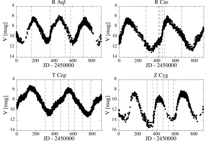
Figure 1: The light curves obtained by AAVSO (Mattei Mattei99 (1999)). The epochs of the ISO observations are denoted as dotted lines.

2.1 An overview of the observed spectra

The observed spectra are shown in Fig. 3. The positions of the major molecular bands are indicated. Due to their large optical depth (Fig. 2), H₂O features dominate both the global shape and the small features between 2.5 and 4.0 $\mu$m. CO₂ bands are visible at 2.67 $\mu$m. OH absorption features are seen around 3.5 $\mu$m in R Aql and T Cep, especially near maximum, while these features are not clear in R Cas and Z Cyg.

All of the four stars indicate periodical variations. The 2.7 $\mu$m absorption relative to the maximum flux around 3.5 $\mu$m is generally shallower around maximum than minimum. The flux levels return to a comparable level after one period, for example, in T Cep ($\phi$=0.58, 1.39, and 1.61) and in Z Cyg ($\phi$=0.55, and 1.63).

Representative ISO/SWS spectra in the 3.8 $\mu$m region are shown in Fig. 4. There are three conspicuous features which show time variation. The appearance of these features is inverse from minimum to maximum. As we will discuss in Sect. 3.2.2, the features denoted with ‘x’ are in absorption and the ones with ‘y’ are in emission. The definition of the absorption or emission at 3.88 $\mu$m is opposite to the aspect.

Figure 2: ¹H${}_{2}^{16}$O optical depth ($\tau$) calculated from the line list of Partridge & Schwenke (Partridge97 (1997)). Parameters are a line width of 5 km s^-1, a column density of $3\times 10^{21}$ cm^-2 multiplied by isotopic abundance ratio (0.997), and an excitation temperature of 2000 K. H₂O lines continuously occupy the spectrum in the 2.5–5.0 $\mu$m region. These lines are mainly the vibrational transitions of $\Delta v_{1}=1$, $\Delta v_{2}=2$, and $\Delta v_{3}=1$ (Table 3). (Author note: This figure is modified from the original A&A version, due to the restriction of file size of astro-ph. The optical depth is smoothed with a resolution of R=2000.)

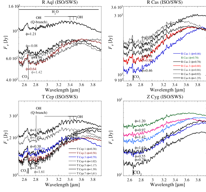
Figure 3: ISO/SWS spectra. The optical variability phase ($\phi$), which is estimated from AAVSO light curve (Mattei Mattei99 (1999)) at each observation, is indicated by the labels. The 2.7 $\mu$m absorption with respect to the flux maximum around 3.5 $\mu$m is generally shallower around maximum than minimum. The flux levels return to a comparable level after one period. There are two spectra for $\phi$=0.78 (on the same day) for R Cas, and only R Cas in the program of VARLPV is plotted.

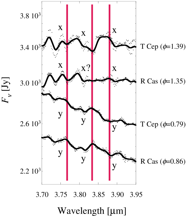
Figure 4: Representative ISO/SWS spectra in the 3.8 $\mu$m region. Three conspicuous features, which show time variation, are marked as ‘x’ and ‘y’. These features are inverted between the spectra of T Cep ($\phi$=1.39) and R Cas ($\phi$=1.35) and the ones of T Cep ($\phi$=0.79) and R Cas ($\phi$=0.86). As we discuss in Sect. 3.2.2, ‘x’ is an absorption phase and ‘y’ is an emission phase of the feature. The feature at 3.88 $\mu$m is opposite to its aspect. The flux of T Cep is scaled by a factor of 1.5. The dots are ISO/SWS data sampling points before re-gridding to constant wavelength grid. Although there is a scatter in the data presented, we could demonstrate that the phases of the features are correct and height of the features generally have uncertainty of up to 10 %.

3 Model analysis

3.1 Two-layer ‘slab’ model

Water spectra in Mira variables are well represented by a model consisting of two water layers (Yamamura et al. 1999b ). In $o$ Cet, one layer contributes to the emission features longer than $\sim$3.5 $\mu$m, and the other layer contributes to the absorption features shorter than $\sim$3.5 $\mu$m. These two layers are called ‘hot’ layer and ‘cool’ layer, respectively.

We use the same model as Yamamura et al. (1999b ). Plane-parallel, disk shape (or circular slabs), uniform molecular layers are superposed, and the radiative transfer through the layers is calculated. A schematic view of this model configuration is indicated in Fig. 5. Each layer is described by three parameters, the excitation temperature ($T_{\mathrm{hot}}$ or $T_{\mathrm{cool}}$), the column density ($N_{\mathrm{hot}}$ or $N_{\mathrm{cool}}$), and the radius of the layer ($R_{\mathrm{hot}}$ or $R_{\mathrm{cool}}$). The radii of the layers are given relative to $R_{*}$, the radius of the background continuum source.

The ‘hot’ layer has an excitation temperature of about 2000 K. The water spectrum longer than $\sim$3.5 $\mu$m is dominated by this ‘hot’ layer (seen in Fig. 7, for example). The H₂O lines in this wavelength region are mainly caused by higher excitation levels of $\Delta v_{2}=2$, $\Delta v_{1}=1$, and $\Delta v_{3}=1$. The upper ‘cool’ layer has an excitation temperature of 1000–1400 K and is seen below $\sim$3.5 $\mu$m, where relatively low excitation levels of $\Delta v_{1}=1$ and $\Delta v_{3}=1$ dominate. This ‘cool’ layer becomes optically thick below $\sim$3.5 $\mu$m for a column density of $1\times 10^{20}$–$1\times 10^{21}$ cm^-2 (Table 4). The column densities in Mira variables usually exceed these values (Yamamura et al. 1999b ; summarized in Table 5). Thus, the features from the ‘hot’ layer are masked by the ‘cool’ layer below $\sim$3.5 $\mu$m.

The ‘disk shape’ plane-parallel model (Fig. 5) is a simplification of the spherical geometry. This simplification enables us to treat more than one million H₂O lines. The validity of this disk simplification will be discussed later by comparison with spherical models (Sect. 3.4).

We note that ‘two layer slab model’, or even spherically geometric two layer model, does not describe the physics in the atmosphere of the star. These models are used to fit the observed spectra, and to interpret the observational results. Two layers are assumed to be independent and discontinuous without any interaction, which are unlikely in the real atmosphere.

For the energy level populations of the molecules, local thermodynamic equilibrium (LTE) is assumed. A turbulent velocity of 5 km s^-1 is assumed for all the molecules (see Yamamura et al. 1999b ). The line list of H₂O is taken from Partridge & Schwenke (Partridge97 (1997)) and the isotope ratio from HITRAN 1996 (Rothman et al. Rothman99 (2001)) is applied. The line lists of OH and CO₂, which are used for data-analysis, are also taken from HITRAN.

Table 3: H₂O bands of main isotope in near-infrared region (Herzberg Herzberg45 (1945)). H₂O has three vibrational levels; symmetric stretch ($v_{1}$), bending of the OH bond ($v_{2}$), and asymmetric stretch ($v_{3}$). The lower state of vibrational levels is 0,0,0 for all bands.

Band centre		Upper state
[cm-1]	[$\mu$m]	$v_{1}$	$v_{2}$	$v_{3}$
1594.8	6.270	0	1	0
3151.4	3.173	0	2	0
3657.1	2.734	1	0	0
3755.8	2.663	0	0	1

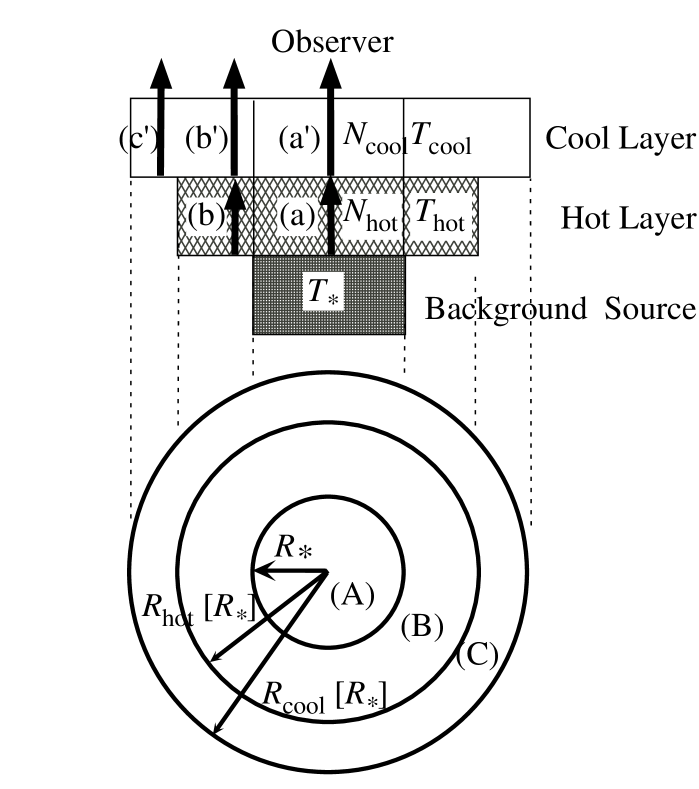
Figure 5: Model configuration. Two disk-shape molecular layers are superposed on a background source, and the radiative transfer is solved though the layers. The top panel indicates the side view and the bottom panel indicates the geometry seen by the observer.

Table 4: The approximate H₂O column densities where optical depth $\tau$ becomes unity at each wavelength. The turbulent velocity is 5 km s^-1.

$T_{\mathrm{ex}}$	$N_{\mathrm{\tau}_{3.8\,\mu m}=1}$	$N_{\mathrm{\tau}_{3.5\,\mu m}=1}$	$N_{\mathrm{\tau}_{3.2\,\mu m}=1}$	$N_{\mathrm{\tau}_{2.5\,\mu m}=1}$
	[cm-2]	[cm-2]	[cm-2]	[cm-2]
2000	$5.5\times 10^{21}$	$1.4\times 10^{21}$	$3.5\times 10^{20}$	$1.3\times 10^{20}$
1400	$2.4\times 10^{22}$	$3.4\times 10^{21}$	$7.6\times 10^{20}$	$1.2\times 10^{20}$
1200	$4.9\times 10^{22}$	$5.4\times 10^{21}$	$1.0\times 10^{21}$	$1.3\times 10^{20}$
1000	$1.1\times 10^{23}$	$1.0\times 10^{22}$	$1.3\times 10^{21}$	$1.5\times 10^{20}$
800	$3.3\times 10^{23}$	$2.6\times 10^{22}$	$1.7\times 10^{21}$	$2.1\times 10^{20}$
600	$1.6\times 10^{24}$	$1.1\times 10^{23}$	$2.1\times 10^{21}$	$3.7\times 10^{20}$
400	$1.6\times 10^{25}$	$1.2\times 10^{24}$	$2.3\times 10^{21}$	$1.3\times 10^{21}$

Table 5: Results derived by Yamamura et al. (1999b ).

Name	$T_{\mathrm{hot}}$	$T_{\mathrm{cool}}$	log $N_{\mathrm{hot}}$	log $N_{\mathrm{cool}}$	$R_{\mathrm{hot}}$	$R_{\mathrm{cool}}$
	[K]	[K]	[cm-2]	[cm-2]	[$R_{*}$]	[$R_{*}$]
$o$ Cet	2000†	1400	21.0	20.5	2.0	2.3
Z Cas	2000†	1200	22.0	21.0	1.1	1.7

^† assumed.

3.2 The model parameters

We calculated more than 50 000 spectra covering a wide range of parameters in order to fit the observed spectra, using the $\chi^{2}$ analysis. The ranges and step sizes of the calculated parameters are summarized in Table 6. There are seven parameters. $T$, $N$, $R$ of the ‘hot’ and ‘cool’ layers are given independently. The background continuum is assumed to be a blackbody of temperature $T_{*}$ of 3000 K. In the following section the effects of each parameter on the spectra are described in detail. We emphasize that the radius of the hot layer ($R_{\mathrm{hot}}$) is an essential parameter for the variation between absorption and emission at wavelengths longer than $\sim$3.8 $\mu$m. The other parameters are less important to the features in this wavelength range. In the following figures (Figs. 6–10) the model spectra are presented for a star at a distance of 100 pc and with a radius $R_{*}$ of $3\times 10^{13}$ cm.

Table 6: The ranges of the parameters for $\chi^{2}$ analysis.

Parameter	Values	Grid	Comments
$T_{*}$ [K]	3000		Fixed
$T_{\mathrm{hot}}$ [K]	2000		Fixed
$T_{\mathrm{cool}}$ [K]	1000–1400	100
log $N_{\mathrm{hot}}$[cm-2]	20.00–23.00	0.25
log $N_{\mathrm{cool}}$[cm-2]	20.00–23.00	0.25
$R_{\mathrm{hot}}$[$R_{*}$]	1.0–3.0	0.2	$R_{\mathrm{hot}}$$<$$R_{\mathrm{cool}}$
$R_{\mathrm{cool}}$[$R_{*}$]	1.0–3.0	0.2
	3.0–4.5	0.5

3.2.1 The spectrum of the central star as background source

Generally, the column densities of H₂O layers in Mira variables (e.g. Yamamura et al. 1999b ) give optically thick layers at most wavelengths under consideration. In Fig. 6, we show calculated H₂O spectra with various temperatures ($T_{*}$) of the blackbody as a background spectrum of H₂O, and we examine the resultant dependence of H₂O bands on the background source. This figure demonstrates that the effects of the background source only appear at wavelengths longer than $\sim$3.5 $\mu$m where the optical depth of H₂O becomes small. In the present analysis, we assume that the background spectrum is a blackbody with temperature $T_{*}$=3000 K, since it is difficult to determine this parameter.

Figure 6: The effects of $T_{*}$ on the spectra are shown. The thick lines indicate the synthetic spectra with a two-layer ‘slab’ model, and the dotted lines indicate the background continuum level for each $T_{*}$. From top to bottom, $T_{*}$=3000, 2800, 2600, 2400, 2200 K. Other parameters are fixed as $T_{\mathrm{hot}}$=2000 K, $T_{\mathrm{cool}}$=1200 K, $R_{\mathrm{hot}}$=1.0 $R_{*}$, $R_{\mathrm{cool}}$=1.4 $R_{*}$, $N_{\mathrm{hot}}$=$1\times 10^{22}$ cm^-2, and $N_{\mathrm{cool}}$=$1\times 10^{21}$ cm^-2. Due to the large optical depth of H₂O molecules, the difference in background appears only above $\sim$3.5 $\mu$m.

3.2.2 The radius of the hot layer

In Fig. 7, the influence of $R_{\mathrm{hot}}$ is shown. The features in the region longer than $\sim$3.5 $\mu$m vary with $R_{\mathrm{hot}}$. The spectrum shorter than $\sim$3.5 $\mu$m is dominated by the absorption by the overlaid ‘cool’ layer and is insensitive to the parameters of the hot layer. When $R_{\mathrm{hot}}$ is $\approx$1.6 $R_{*}$ with $T_{\mathrm{hot}}$=2000 K, the emission from the outer part of the layer ($r>R_{*}$) fills up the absorption originating in the inner part of the layer ($r<R_{*}$) and the spectrum becomes almost flat at wavelengths longer than 3.5 $\mu$m. Emission features appear when $R_{\mathrm{hot}}$ becomes larger than $\approx$1.6 $R_{*}$. The effects are most prominently seen in the 3.83 $\mu$m feature in the top panel of Fig. 7. Also the slope in the 3.8 $\mu$m region depends on $R_{\mathrm{hot}}$. The 3.8 $\mu$m region is enlarged in the bottom panel of Fig. 7. In this plot, not only the 3.83 $\mu$m feature but also other two features at 3.77 $\mu$m and 3.88 $\mu$m are marked. These three marked features are in emission, when the features arising from the outer disk of $R_{\mathrm{hot}}$$>r>R_{*}$ (region B in Fig. 5) exceed the absorption arising from the inner disk of $r<R_{*}$ (region A in Fig. 5); this is marked as ‘y’ in the figures. As the features arising from $r<R_{*}$ are dominant, the features are inverted and we indicate the features as ‘x’. These three features are not formed by a single H₂O line but by a combination of a large number of overlapping H₂O lines. The definition of the emission and absorption features is opposite for the 3.88 $\mu$m feature, as this feature is formed by slightly smaller optical depth compared to the neighboring regions.

Figure 7: Upper: The radius of the ‘hot’ layer ($R_{\mathrm{hot}}$) with an excitation temperature ($T_{\mathrm{hot}}$) of 2000 K influences the features longer than $\sim$3.5 $\mu$m. The solid lines are by two-layer model and the dotted lines are only by the hot layer. The effects are most prominently seen in the 3.83 $\mu$m feature, which is either seen in emission or in absorption depending on $R_{\mathrm{hot}}$. In this case, features longer than $\sim$3.5 $\mu$m change, and become emission when $R_{\mathrm{hot}}$ is larger than $\approx$1.6 $R_{*}$. Other parameters are $T_{*}$=3000 K, $T_{\mathrm{hot}}$=2000 K, $T_{\mathrm{cool}}$=1200 K, $N_{\mathrm{hot}}$=$1\times 10^{22}$ cm^-2, $N_{\mathrm{cool}}$=$1\times 10^{21}$ cm^-2. $R_{\mathrm{cool}}$ is given as $\mbox{$R_{\mathrm{cool}}$}^{2}=\mbox{$R_{\mathrm{hot}}$}^{2}+1^{2}$ [$R_{*}^{2}$]. Lower: The spectra of 3.8 $\mu$m region are enlarged. Conspicuous three features are marked. Note that a feature at 3.88 $\mu$m shows ‘emission like’ feature when spectra are in absorption (see text).

3.2.3 The excitation temperature

The observed spectrum of $o$ Cet suggests that $T_{\mathrm{hot}}$ must be above $\sim$1600 K; below $\sim$1600 K, the flux level of the synthesized spectra shortward of 2.5 $\mu$m is lower than the flux levels of the observed spectra. Because the spectrum of the optically thick hot H₂O layer behaves like a blackbody with temperature of $T_{\mathrm{hot}}$, the flux level around 2.5 $\mu$m decreases considerably below 1600 K. Thermal equilibrium chemistry shows that H₂O molecules are abundant below $\sim$2200 K in the atmosphere of red giants and that the H₂O abundance decreases significantly above this temperature (Tsuji Tsuji64 (1964)). The hot layer is expected to have an excitation temperature in the range of $1600<\mbox{$T_{\mathrm{hot}}$}<2200$ K. With the resolution of 300 it is difficult to determine $T_{\mathrm{hot}}$. Thus, we fix $T_{\mathrm{hot}}$ as 2000 K.

When the hot layer produces emission features, the emergent H₂O features always appear similar (Fig. 8). We calculated model spectra with $T_{\mathrm{hot}}$ of 1800 K and 2000 K and confirmed that the other parameters were only little affected. $R_{\mathrm{hot}}$ becomes systematically larger by 0.2 $R_{*}$ at most (1 parameter step of $R_{\mathrm{hot}}$) at $T_{\mathrm{hot}}$=1800 K compared to $T_{\mathrm{hot}}$=2000 K.

Figure 8: The effects of $T_{\mathrm{hot}}$ for the case where the hot H₂O is seen in emission. From top to bottom $T_{hot}$=2000, 1800, 1600 K. Full lines show the spectra with two-layers, and dotted lines show the spectra only with the hot layer as a background of the ‘cool’ layer. Other parameters are $T_{*}$=3000 K, $T_{\mathrm{cool}}$=1200 K, $R_{\mathrm{hot}}$=2.2 $R_{*}$, $R_{\mathrm{cool}}$=2.4 $R_{*}$, $N_{\mathrm{hot}}$=$1\times 10^{22}$ cm^-2, $N_{\mathrm{cool}}$=$1\times 10^{21}$ cm^-2.

3.2.4 The column density

Fig. 9 shows that $N_{\mathrm{hot}}$ changes the spectra moderately. The noticeable features around 3.8 $\mu$m (Sect. 3.2.2) are seen when $N_{\mathrm{hot}}$ is in the range of $1\times 10^{21}$–$3\times 10^{22}$ cm^-2. Below or above this range these feature are not detectable at the current wavelength resolution.

The wavelengths shorter than 2.7 $\mu$m are dominated by the lines in the R-branches, while the lines in P-branches start at longer wavelengths. The gap between the two branches is seen as an ‘emission-like feature’ at 2.7 $\mu$m. The column density of the cool layer ($N_{\mathrm{cool}}$) determines the feature around 2.7 $\mu$m (Fig. 10). T Cep and R Aql, with column densities in the order of $10^{20}$–$10^{21}$ cm^-2 show the feature. R Cas and Z Cyg, whose features around 2.7 $\mu$m cannot be clearly seen, have higher column densities than this range.

Figure 9: The effects of $N_{\mathrm{hot}}$ on the spectra when hot H₂O is seen in emission. The solid lines are for two-layer model and the dotted lines are only for the hot layer. From top to bottom $N_{H}$=$3\times 10^{22},1\times 10^{22},3\times 10^{21},1\times 10^{21},3\times 10^{20},1\times 10^{20}$ cm^-2. Other parameters are $T_{*}$=3000 K, $T_{\mathrm{hot}}$=2000 K, $T_{\mathrm{cool}}$=1200 K, $R_{\mathrm{hot}}$=1.8 $R_{*}$, $R_{\mathrm{cool}}$=2.0 $R_{*}$, $N_{\mathrm{cool}}$=$1\times 10^{21}$ cm^-2.

Figure 10: The influence of $N_{\mathrm{cool}}$ on the spectrum. The solid lines are for two-layer model and the dotted line is for the hot layer as the background of the cool layer. From top to bottom, $N_{\mathrm{cool}}$=$1\times 10^{20},3\times 10^{20},1\times 10^{21},3\times 10^{21},1\times 10^{22},3\times 10^{22}$ cm^-2. Other parameters are $T_{*}$=3000 K, $T_{\mathrm{hot}}$=2000 K, $T_{\mathrm{cool}}$=1200 K, $R_{\mathrm{hot}}$=1.8 $R_{*}$, $R_{\mathrm{cool}}$=2.0 $R_{*}$, $N_{\mathrm{hot}}$=$1\times 10^{22}$ cm^-2.

3.3 Other molecules in this wavelength range

3.3.1 OH

There are sharp OH bands visible in some spectra of R Aql and T Cep, especially around visual maximum. The Q-branch lines at 2.8 $\mu$m do not appear strongly in the observed spectra (Fig. 3). This is because H₂O with its large optical depth masks the OH Q-branch lines in the 2.8 $\mu$m region.

In the current analysis, we include OH molecules only in the cool layer, and we assume that the excitation temperature and radius for OH molecules are the same as that of cool H₂O layer so as to reduce the number of the parameters. We confirm that the H₂O parameters are not changed by more than the typical uncertainties by including OH molecules.

OH molecules can persist up to 4000 K, which is higher temperature than for H₂O (Tsuji Tsuji64 (1964)). The assumption of the OH excitation temperature in our model is not ideal. The OH lines with higher excitation temperature than the hot H₂O layer are not seen in the model spectra due to large opacity of H₂O. We ignore OH with higher excitation temperature.

3.3.2 CO₂

¹²C¹⁶O₂ absorption of the $10^{0}1$–$00^{0}0$ and $02^{0}1$–$00^{0}0$ vibration bands (Herzberg Herzberg45 (1945)) is seen at 2.7 $\mu$m. The CO₂ spectrum of Z Cyg ($\phi=0.79$) is indicated in Fig. 11. CO₂ molecules are superposed over the two H₂O layers. The feature at 2.67 $\mu$m is reproduced well by CO₂. The parameters of the synthetic CO₂ spectrum in Fig. 11 are an excitation temperature of 800 K, a column density of $1\times 10^{19}$ cm^-2, and a radius of 4.0 $R_{*}$. These parameters are estimates only. We mask the wavelength region of 2.65–2.75 $\mu$m for the $\chi^{2}$ analysis of the H₂O fitting and do not discuss the CO₂ molecules in this paper.

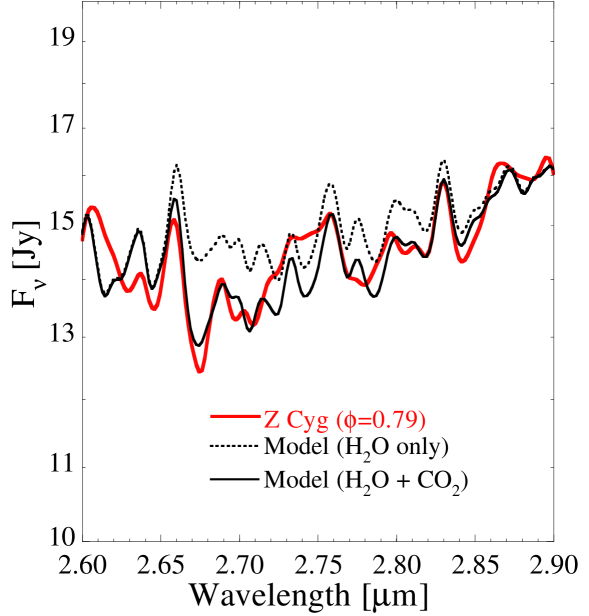
Figure 11: CO₂ features around 2.7 $\mu$m. An example is the spectrum in Z Cyg-2 ($\phi$=0.79). We put one extra CO₂ layer over the cool H₂O layer in the ‘slab’ model. The parameters of synthetic CO₂ spectrum are estimated to be excitation temperature of 800 K, a column density of $1\times 10^{19}$ cm^-2, and a radius of 4.0 $R_{*}$. The parameters of H₂O are listed in Table 8.

3.3.3 SiO

SiO $\Delta v$=2 bands at 4.1 $\mu$m region are present in the SWS spectra. The $\Delta v$=3 vibration levels around 3 $\mu$m region are not clear. We mask the wavelengths longer than 3.95 $\mu$m in the $\chi^{2}$ analysis in order to avoid the influence of the SiO molecules.

3.4 Spherical effects

We adopted disk-shape plane-parallel models to calculate a number of spectra with various parameter sets for the $\chi^{2}$ analysis. We examine the parameters derived from the ‘slab’ model. In order to validate this simplification, spectra of spherical models are compared with ‘slab’ model spectra using the same $\chi^{2}$ analysis. In the spherical geometry, two H₂O layers with uniform temperatures are adopted. The density gradient in each layer is assumed to vary as $r^{-2}$. An example is indicated in Table 7. The parameters are consistent between these two models. The results derived from the simple disk model can provide fairly good estimates of the structure of the outer layers. This is because the optical depth of the H₂O layer is so high (optical depth at 3.5 $\mu$m becomes about unity with a column density of $1\times 10^{21}$ cm^-2 and an excitation temperature of 2000 K; Table 4), that only the surface of each sphere is important for the synthetic spectra. The radius where the optical depth becomes thick in a spherical model is represented as the radius of the ‘slab’ model. If we compare the spectra with these two geometric models in an optically thin case (say column density of $10^{18}$–$10^{19}$ cm^-2), we find larger discrepancies.

Table 7: Validation of a ‘slab’ model as a simplification of spherical model. A spectrum of spherical model is compared with ‘slab’ model using the $\chi^{2}$ analysis. $R_{\mathrm{in}}$ and $R_{\mathrm{out}}$ are the inner boundary and the outer boundary of the spherical model, respectively. $T_{\mathrm{hot}}$ is 2000 K for both models.

	$T_{\mathrm{cool}}$	$R_{\mathrm{hot}}$		$R_{\mathrm{cool}}$		$N_{\mathrm{hot}}$	$N_{\mathrm{cool}}$
	[K]	[$R_{*}$]		[$R_{*}$]		[cm-2]	[cm-2]
		$R_{\mathrm{in}}$	$R_{\mathrm{out}}$	$R_{\mathrm{in}}$	$R_{\mathrm{out}}$
Spherical	1400	1.0	2.2	2.2	3.0	$3\times 10^{21}$	$3\times 10^{20}$
‘Slab’	1400	2.0		2.8		$3\times 10^{21}$	$3\times 10^{20}$

3.5 Fitting process

The best fit for each observed spectrum is derived by the $\chi^{2}$ analysis. The spectral resolution is 300–500 in these wavelengths. All the spectra are convolved by a Gaussian with the wavelength resolution of $\lambda/\Delta\lambda=300$. $\chi_{m}^{2}$ is the reduced $\chi^{2}$, and divided by the degrees of freedom $m$. The best parameter sets are found by minimizing $\chi_{m}^{2}$. The wavelength range 2.5–3.95 $\mu$m is used except for the 2.65–2.75 $\mu$m region which is strongly affected by CO₂ bands.

The SWS scans the same wavelength region twice. The difference between two scans is a good indication of the observational uncertainty. Two scans are normally consistent within 0.6 % of the flux over 2.5–4.0 $\mu$m. In some observations AOT bands 1D and 1E (3.5–4.0 $\mu$m) show a significant difference between two scans. The difference is as large as 10 % of the flux in the worst case (R Aql-1; we discard this observation from the later discussions). We added this difference in flux and 1 % of the flux, which represents the scatter of the data around the re-gridded data, to an observational error, $\sigma$. The latter part is necessary to avoid $\chi^{2}$ diverging to the infinity. The error of each parameter is obtained by calculating grid points within 3 $\sigma$ level from the parameter of the best $\chi^{2}$, when other parameters are fixed. The error of our fit is not a continuous function but rather a grid scale.

4 Results

4.1 The best-fit spectra and their parameters

The best fit synthetic spectra corresponding to the observed spectra (Fig. 3) are shown in Fig. 12. Our simple ‘slab’ model reproduces the global shape of the observed spectra. Residuals between the observed spectra and the fitted spectra are shown in Fig. 12. The fit is as good as a few % in the most of the investigated spectral range and about 10 % at the worst part. The 3.8 $\mu$m region of the observed spectra and the model spectra is enlarged in Fig. 13. The variation with phase in the three conspicuous features is seen in the observed spectra, and these features are reproduced by the model except at $\phi$=0.78 and 0.80 of R Cas (R Cas, R Cas-2, R Cas-3). The small features of the observed spectra are generally reproduced in respect to the trend of emission or absorption. However, the detailed shapes of the small features (e.g. height or width) are sometimes not fitted well. This implies that two layer slab model is too simple approximation and the atmospheric structure is more complicated in Mira variables.

The parameters of the best fit spectra are listed in Table 8. All four stars show the common tendency that the radius of the hot layer ($R_{\mathrm{hot}}$) is about 1.0 $R_{*}$ around minimum and about 2.0 $R_{*}$ around maximum (Fig. 14), confirming the suggestion in Yamamura et al. (1999b ). The cool layer is located at about 2.5–4 $R_{*}$. The column density of the cool layer ($N_{\mathrm{cool}}$) varies from object to object rather than showing a trend with the phase and $\log\mbox{$N_{\mathrm{cool}}$}$ ranges from 20.75 cm^-2 to 22.25 cm^-2.

The column density of the hot layer ($N_{\mathrm{hot}}$) has a large uncertainty as discussed in Sect. 3.2.2. From the equivalent width, we could give a lower limit when the features are clearly seen as emission. At the phases with the strongest emission features at 3.83 $\mu$m in each star (R Aql-5 at $\phi$=1.99; R Cas-5 at $\phi$=0.92; T Cep-3 at $\phi$=0.79; Z Cyg-3 at $\phi$=0.97), the column density of the hot layer should be higher than $\approx$$10^{21}$ cm^-2, otherwise the features would not have been detected.

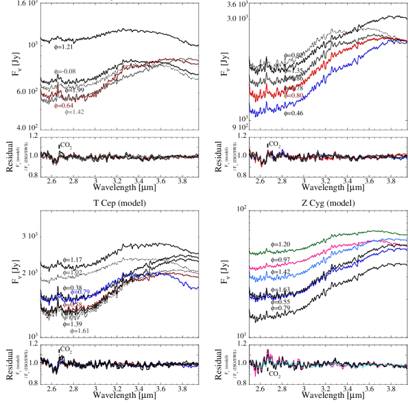
Figure 12: The fitted results and the residuals. Two spectra at $\phi$=0.78 (on the same day) and one spectra at $\phi$=0.80 of R Cas are fitted with the same parameters, and the synthetic spectra are identical.

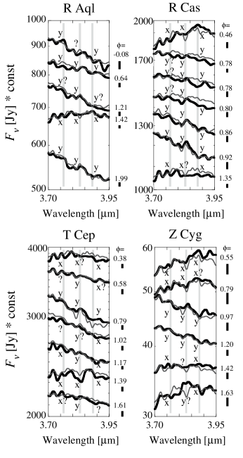
Figure 13: The spectra in the 3.8 $\mu$m region are enlarged; the ISO/SWS spectra (bold lines), and the model spectra (thin line). The three conspicuous features (see Sect. 3.2.2; Fig. 7), which shows time variation, are marked. The mark, ‘x’ shows the absorption phase and ‘y’ shows the emission phase of ISO/SWS spectra. The definition of the emission and absorption feature at 3.88 $\mu$m is opposite to their aspects. Around minimum the features are observed in absorption, while around maximum they are seen in emission. The error bars below the phase indicate $\sigma$ (Sect. 3.5) at 3.83 $\mu$m. Slight wavelength shift of the feature peak is seen, especially in Z Cyg. These shifts seem to be observational errors.

There is an uncertainty remaining in the fits of individual spectra. The spectra of R Cas, R Cas-2, R Cas-3, which were taken within 2 weeks, are fitted by the same parameter sets. These three synthetic spectra based on $\chi^{2}$ analysis show absorption features in the 3.8 $\mu$m region. However, all of them show emission features in the observed spectra (Fig. 13). Thus, the fitted parameters for these three spectra are not reliable. Also the features in the 3.8 $\mu$m region in Z Cyg-6 are not reproduced with the best parameters. However, the data of Z Cyg-6 are not affected by the instrumental error; the features in the 3.8 $\mu$m region in Z Cyg-6 seem to be real. Thus, the parameters of Z Cyg-6 are doubtful.

In some phases, the features in the 3.8 $\mu$m region do not clearly appear in the observed spectra, for example, in T Cep-2 ($\phi$=0.58). There are at least three solutions: (1) The column density of the hot layer is extremely high, and the H₂O lines are completely saturated. (2) The radius of the hot layer just falls at $\approx$1.6 $R_{*}$ where the contributions of emission fills up the absorption features. (3) The hot layer disappears, i.e. the column density of the hot layer is so low that the features are undetectable. We cannot distinguish the three cases from the observed spectra. Although the $\chi^{2}$ analysis suggests that case (1) is the most likely for most of such spectra, cases (2) and (3) cannot not be ruled out.

4.2 The 3.8 $\mu$m region

The most interesting parameter in this study is the radius of the hot layer, $R_{\mathrm{hot}}$. The observed spectra in Fig. 13 indicate that the 3.8 $\mu$m features show emission around maximum and absorption around minimum. This suggests that $R_{\mathrm{hot}}$ is larger than $\approx$1.6 $R_{*}$ around maximum and smaller than that around minimum. The features in emission phase are not always exactly the inverse shape of the absorption features, possibly because of the complicated structure of the atmosphere in Mira variables.

The variation in $R_{\mathrm{hot}}$ derived from the model fitting is plotted in Fig. 14 against the optical phase. In all four cases, $R_{\mathrm{hot}}$ reaches about 2 $R_{*}$ around maximum and becomes $\sim$1 $R_{*}$ around minimum.

There are slight differences among the stars. Z Cyg still shows absorption features at phase 0.79, while the other three stars already show weak emission. This trend appears to be related to the characteristics of the light curve (Fig. 1). The light curve of Z Cyg shows a steep increase and a gradual decrease in the V-band. The visual magnitude of Z Cyg at $\phi$=0.79 is near the minimum, while in other stars the visual magnitudes already start increasing at this phase. Fig. 15 shows $R_{\mathrm{hot}}$ as a function of visual magnitude at each epoch, after subtraction of the maximum magnitude. A separation is found at $\mathrm{V}-\mbox{$\mathrm{V}_{\mathrm{max}}$}$ of 3.0 mag; below that $R_{\mathrm{hot}}$ is $\sim$2 $R_{*}$ and above that $R_{\mathrm{hot}}$ is $1.0\,R_{*}$, indicating the variation in $R_{\mathrm{hot}}$ is connected with variability. One of the classification criteria of Mira variables is that visual amplitude is larger than 2.5 mag. Fig. 15 implies that the emission features might be related with the large-amplitude pulsating variables.

Table 8: The best fit parameters, and the estimated uncertainties. OH is included in some fits with a fixed column density of $1\times 10^{21}$ cm^-2. The numbers of errors are not given when the errors are smaller than 1 step of the model parameters.

Name	Phase	$T_{\mathrm{cool}}$	$R_{\mathrm{hot}}$	$R_{\mathrm{cool}}$	log $N_{\mathrm{hot}}$	log $N_{\mathrm{cool}}$	log $N_{\mathrm{OH}}$	$\chi_{m}^{2}$
		[K]	[$R_{*}$]	[$R_{*}$]	[cm-2]	[cm-2]	[cm-2]
R Aql-1	$-0.08$	1400	$1.8_{-0.2}^{+0.2}$	$2.4_{-0.2}^{+0.2}$	21.75${}_{-0.50}^{+0.50}$	$21.25_{-0.50}^{+1.00}$		1.1
R Aql-2	0.64	1400	2.2	$2.6^{+0.2}$	22.50${}_{-0.25}^{+0.50}$	$21.25_{-0.25}^{+0.25}$		2.5
R Aql-3	1.21	1400	$2.0^{+0.2}$	$3.0_{-0.2}$	22.25${}_{-0.25}^{+0.75}$	$20.75_{-0.50}^{+0.50}$	21	2.2
R Aql-4	1.42	1200	$1.2_{-0.2}^{+0.2}$	2.4	21.50${}_{-0.75}^{+0.25}$	$21.50_{-0.50}^{+1.25}$		2.4
R Aql-5	1.99	1400	$2.0_{-0.2}^{+0.2}$	$2.6^{+0.2}$	21.75${}_{-0.25}^{+0.25}$	$21.50_{-0.25}^{+0.75}$	21	1.5
R Cas-1	0.46	1100	1.2	2.4	21.75${}_{-0.50}^{+0.25}$	$22.00_{-0.25}^{+0.75}$		2.7
R Cas	0.78	1000	$1.0^{+0.4}$	3.5	20.75${}_{-0.75}^{+0.25}$	$22.00_{-0.25}^{+0.25}$		2.9
R Cas-2	0.78	1000	$1.0^{+0.4}$	3.5	20.75${}_{-0.75}^{+0.50}$	$22.00_{-0.25}^{+0.25}$		3.1
R Cas-3	0.80	1000	$1.0^{+0.6}$	3.5	20.75${}_{-0.75}^{+0.25}$	$22.00_{-0.25}^{+0.25}$		3.2
R Cas-4	0.86	1200	2.2	3.5	22.25${}_{-0.25}^{+0.50}$	$21.75_{-0.25}^{+0.50}$		2.5
R Cas-5	0.92	1100	$2.2^{+0.2}$	4.5	22.25${}_{-0.25}^{+0.75}$	$21.50_{-0.25}^{+0.25}$		2.3
R Cas-6	1.35	1100	$1.2^{+0.2}$	2.6	21.50${}_{-0.75}^{+0.25}$	$21.50_{-0.25}^{+0.25}$		3.1
T Cep-1	0.38	1200	$1.0^{+0.4}$	2.4	21.00${}_{-0.50}^{+0.25}$	$21.50_{-0.50}^{+0.50}$		4.1
T Cep-2	0.58	1300	1.8	2.6	22.50${}_{-0.50}^{+0.50}$	$21.50_{-0.25}^{+0.50}$		2.2
T Cep-3	0.79	1300	$1.8_{-0.2}^{+0.2}$	2.6	21.50${}_{-0.50}^{+0.25}$	$21.50_{-0.25}^{+0.25}$	21	2.3
T Cep-4	1.02	1300	1.8	3.0	22.00${}_{-0.25}^{+0.50}$	$21.50_{-0.50}^{+0.75}$	21	2.5
T Cep-5	1.17	1400	1.8	2.4	22.00${}_{-0.25}^{+0.50}$	$21.25_{-0.25}^{+0.50}$	21	3.4
T Cep-6	1.39	1200	$1.2_{-0.2}^{+0.2}$	2.2	21.25${}_{-1.00}^{+0.25}$	$21.50_{-0.25}^{+0.50}$		3.7
T Cep-7	1.61	1000	$1.0^{+0.2}$	3.5	20.75${}_{-0.25}^{+0.25}$	$21.50_{-0.25}^{+0.25}$		2.7
Z Cyg-1	0.55	1100	1.2	2.2	21.75${}_{-0.50}^{+0.25}$	$22.00_{-0.25}^{+0.75}$		2.7
Z Cyg-2	0.79	1000	$1.2_{-0.2}^{+0.2}$	$2.8_{-0.2}$	21.50${}_{-1.00}^{+0.25}$	$22.25_{-0.25}^{+0.50}$		3.0
Z Cyg-3	0.97	1200	$2.4^{+0.2}$	4.0	22.25${}_{-0.25}^{+0.75}$	$22.00_{-0.25}^{+0.50}$		1.5
Z Cyg-4	1.20	1300	1.8	2.6	22.00${}_{-0.50}^{+1.00}$	$21.75_{-0.25}^{+0.50}$		1.2
Z Cyg-5	1.42	1100	$1.2_{-0.2}^{+0.2}$	2.6	21.00${}_{-1.00}^{+0.50}$	$22.00_{-0.25}^{+0.50}$		2.3
Z Cyg-6	1.63	1100	$1.2_{-0.2}^{+0.2}$	2.2	21.50${}_{-0.75}^{+0.50}$	$22.00_{-0.25}^{+0.50}$		3.0

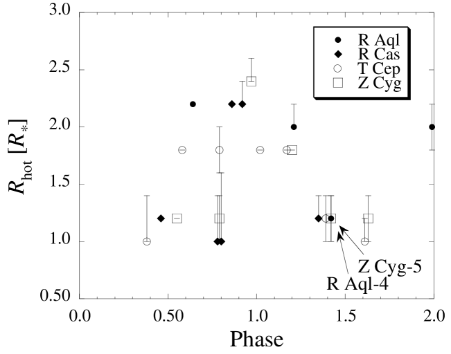
Figure 14: The time variation in the radius of the hot layer ($R_{\mathrm{hot}}$). When $R_{\mathrm{hot}}$ is larger than 1.6 $R_{*}$, the spectrum around 3.8 $\mu$m is in emission, while $R_{\mathrm{hot}}$ smaller than 1.6 $R_{*}$ indicate absorption features. All four stars indicate about 2.0 $R_{*}$ around maximum and about 1.0 $R_{*}$ around minimum.

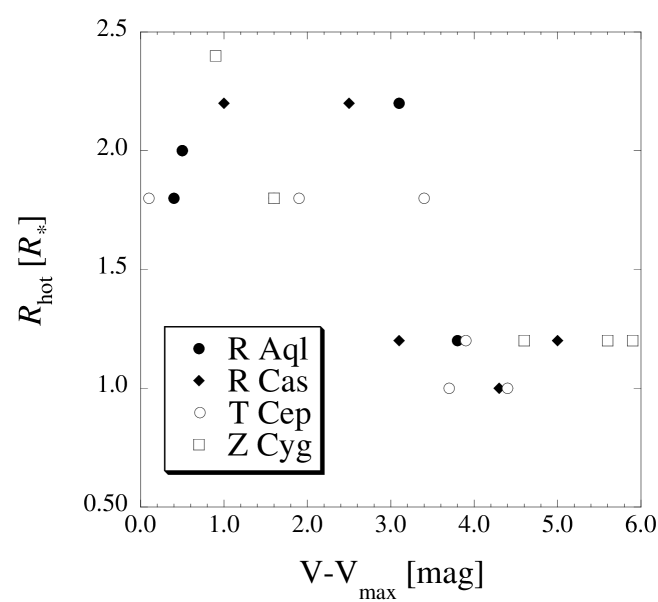
Figure 15: $R_{\mathrm{hot}}$ as a function of visual magnitude at each epoch subtracted from maximum magnitude. There is a separation; when $\mathrm{V}-\mbox{$\mathrm{V}_{\mathrm{max}}$}$ is larger than 3.0 mag $R_{\mathrm{hot}}$ is $\sim$1.0 $R_{*}$, and smaller than 3.0 mag it is $\sim$2.0 $R_{*}$.

5 Discussion

5.1 The dynamical motion in the extended atmosphere

The spectra of H₂O bands in the 3.8 $\mu$m region are reproduced well assuming $T_{\mathrm{hot}}$=2000 K. That temperature indicates that the hot layer traces a relatively inner part of the extended atmosphere. The variation in $R_{\mathrm{hot}}$ indicates the variability of the structure in this region.

The variation in $R_{\mathrm{hot}}$ can be interpreted by the variation in the density structure in the extended atmosphere due to pulsations. Pulsations create local high-density shells or shocks in the extended atmosphere. If the gas temperature in the shock is high enough to dissociate H₂O molecules, they are re-formed behind the shock front: in this case $R_{\mathrm{hot}}$ traces the region with the highest H₂O density located behind the shock front. Duari et al. (Duari99 (1999)) indicated that H₂O can be reformed in a post-shock region. If the shock is moderate and H₂O molecules do not dissociate, the H₂O density increases at the shock front and $R_{\mathrm{hot}}$ traces the motion of the shock front. In either case, the variation in $R_{\mathrm{hot}}$ traces the motion of shocks.

Around minimum, a high H₂O density shell is created by the pulsation shock near the stellar surface; the area of the extended region is smaller, and the contribution of the emission component originating from the extended region is weaker than the absorption component (Fig. 16). Toward maximum, the high H₂O density shell moves away from the stellar surface. The hot layer is extended and emission is observed. This high density shell continues to expand after the maximum, but its temperature and density decrease. The contribution of this shell to the features in the 3.8 $\mu$m region gradually decreases. At the next minimum, a new shock is formed on the surface and produces the absorption features.

The radius of the hot layer is measured in units of $R_{*}$; the radius of the background continuum source (in practice, a 3000 K blackbody). It is uncertain how the stellar radius varies with phase. Interferometric observations show that the stellar radius of Mira variables is rather stable, and varies only by less than 7 % at 902 nm, a wavelength little contaminated with absorption (Tuthill et al. Tuthill95 (1997)). The Rosseland radius derived from theoretical models (Bessell et al. Bessell96 (1996)) varies by about 20 %; the radius is smallest at maximum. These variations in the stellar radius are smaller than our derived variations in $R_{\mathrm{hot}}$/$R_{*}$, which varies by a factor of two. Thus, the location of the hot H₂O layer actually varies by as much as a factor of 1.5–2.0.

Figure 16: A schematic view of the motion of the high H₂O density shell. From top to bottom, it is in the time-sequence. Around minimum, a high-density shell is located on the surface of the star and H₂O is observed in absorption. The high density shell is moving outwards, and located at $\approx$2 $R_{*}$ around maximum. The emission features arise from the high density region expanded further from the ‘photosphere’. After the maximum, the high density shell continues to go outwards. As the shell is expanded, the temperature and density decreases and its contribution to the spectrum in 3.8 $\mu$m region is getting lower.

Hydrodynamic model calculations indicated that H₂O molecules are in non-LTE (Woitke et al. Woitke99 (1999)). We cannot discard non-LTE excitation for the cause of emission features. Recently, Schweitzer et al. (Schweitzer00 (2000)) developed a method to solve non-LTE for H₂O molecules. Such an effect should be considered for future work.

5.1.1 Comparison with the structural variation in the extended atmosphere traced by other molecules

Hinkle et al. (Hinkle82 (1982), Hinkle84 (1984)) and Lebzelter et al. (Lebzelter99 (1999)) found periodical variations in the near-infrared CO lines in the H-band and K-band of several Mira variables. Hinkle et al. (Hinkle82 (1982), Hinkle84 (1984)) found that the CO $\Delta v=3$ lines, with excitation temperatures of 2200–4000 K, show a P Cyg profile; the blue-shifted emission feature is visible from $\phi$=0.6 to 0.8. The CO column density is lowest around $\phi$=0.85. These variations are clearly different from those of hot H₂O. The dissociation energies of CO and H₂O molecules are 11.09 and 5.11 eV, respectively (Däppen Daeppen99 (1999)). It is reasonable to assume that the CO molecules in Hinkle et al. (Hinkle82 (1982), Hinkle84 (1984)) trace even a hotter region interior to the hot H₂O layers. The authors explained the behavior of the CO lines with the shocks caused by the pulsation. A shock affects the CO layer around $\phi$=0.7. The high density region caused by the shock influences the H₂O layer around maximum. It is qualitatively reasonable that this phase lag of the expected shock penetration appears between the CO and H₂O layers because of the difference in transition energy and binding energy of these molecules.

Yamamura et al. (1999a ) found SO₂ in oxygen-rich Mira variables and examined the time variation. Unlike H₂O, the time variation in the SO₂ band does not correlate with the visual variability but changes from emission to absorption over more than a single period. The location of the SO₂ layer is estimated to be about 4–5 $R_{*}$ in T Cep. It is implied that the inner region in the extended atmosphere (hot H₂O layer) follows the optical variability, but the outer region (SO₂ layer) does not. It cannot be ruled out that the outer region has a longer variability period than the inner region because the pulsation shocks do not directly influence the outer region.

5.1.2 Comparison with the hydrodynamic models

Bessell et al. (Bessell96 (1996)) calculated atmospheres of oxygen-rich Mira variables including hydrodynamics. They show CO line profiles for several transitions. The CO first-overtone (excitation level of 0.2 eV) is seen in emission at $\phi$=0.8–1.0. They explained that the CO emission was produced in the pre- and post-shock region in the inner part of the extended atmosphere. Winters et al. (Winters00 (2000)) calculated the CO line profile for both $\Delta v=1$ and $\Delta v=2$ transitions. CO lines, especially those of $\Delta v=1$, show a P-Cyg profile with a strong emission component. Although their model is calculated for carbon stars, the general trend may be applied to oxygen-rich stars. These theoretical models indicate that CO lines are seen in emission due to the high density regions of CO molecules lifted by the pulsation shocks. The appearance of H₂O lines can be interpreted in a similar manner.

Bessell et al. (Bessell96 (1996)) showed the temperature and density structures in the extended atmosphere. A shock occurs at the photosphere and moves outwards. Only models for the fundamental mode of pulsation can produce shocks in the extended atmosphere. Their models indicated that the temperature does not increase drastically at the shock front (nearly isothermal shock). According to their Z-model (fundamental pulsation mode and luminosity of 6310 $L_{\sun}$), the location of the shock increased by a factor of 1.8 from minimum to maximum. The radius of the H₂O layer measured in our work is a factor of 1.5–2.0 larger around maximum than around minimum. Assuming that the hot H₂O layer traces either the location of shock itself or post-shock region, the approximate scales of the shock propagation are comparable with that model.

Bessell et al. (Bessell96 (1996)) also calculated the temperature and the density around the shock region. The temperature and the density at the shocked region have uncertainties according to Bessell et al. (Bessell96 (1996)). Here, we discuss the post-shock region. They show one example, D-model (fundamental pulsation mode and luminosity of 3470 $L_{\sun}$). According to one of their D-models, the gas temperature is 2000 K and the mass density is $1\times 10^{-11}$ g cm^-3 at the post-shock region at maximum phase. The gas temperature is comparable to the excitation temperature of our hot layer. The H₂O number density becomes $5\times 10^{8}$ cm^-3 if we assume the gas is dominated by H₂ and the abundance ratio of H₂ and H₂O is $10^{-4}$. Our analysis indicates that the column density of the hot layer is required to be higher than $\approx 1\times 10^{21}$ cm^-2 to detect the emission features in the 3.8 $\mu$m region. The density calculated by Bessell et al. (Bessell96 (1996)) exceeds the column density $1\times 10^{21}$ cm^-2 out to 0.1 stellar radii. Here we assume $3\times 10^{13}$ cm for one stellar radius. Thus, the density in Bessell et al. (Bessell96 (1996)) is consistent with our estimate.

Another hydrodynamic model is presented by Woitke et al. (Woitke99 (1999)). Unfortunately, the phase is not given in their work, but a shock with a gas temperature of 2000 K reaches 2 stellar radii. In their model, the H₂O number density at the shock front is only $3\times 10^{5}$ cm^-3. A shell thickness larger than $10^{15}$ cm (more than $\sim$30 stellar radii) is required to reach the H₂O column density of $1\times 10^{21}$ cm^-2. The number density in Woitke et al. (Woitke99 (1999)) is by more than an order of magnitude lower than our results. Their results may be applicable to the observations of irregular variables and semi-regular variables by Tsuji et al. (Tsuji97 (1997)), and not to stronger pulsating stars such as Mira variables.

5.2 The optically thick H₂O layers in oxygen-rich Mira variables and their infrared variability

The near-infrared variability has been measured for Mira variables. For example, the L’-band magnitude of R Aqr varies about 0.6 mag (Le Bertre Lebertre93 (1993)). In our sample, the variations are about a factor of 1.4–2.2 (0.5–0.7 in magnitudes) at L’-band (Table 2). As the opacity is dominated by H₂O in this wavelength range, it is likely that H₂O molecules play an essential role in the flux variation.

From Figs. 6–10, the parameters which drastically vary the absolute flux at 3.8 $\mu$m (the effective wavelength of the L’-band; van der Bliek et al. vanderBliek96 (1996)), are the radius of the hot layer ($R_{\mathrm{hot}}$; see Fig. 7) and the excitation temperature of the hot layer ($T_{\mathrm{hot}}$; see Fig. 8). The variation in $R_{\mathrm{hot}}$ from 1.0 to 2.0 $R_{*}$ induces a variation in the emission by a factor of 4.0. The difference in the flux between $T_{\mathrm{hot}}$=1600 and 2000 K is a factor of two. The flux variation is explained by the larger radius and lower excitation temperature of the high H₂O density shell at maximum compared to minimum.

Tuthill et al. (Tuthill00 (2000)) measured the radius of a Mira variable with interferometry: they mentioned that the radius at 3.1 $\mu$m is larger than those in other near-infrared bands, due to molecular opacity. The hot H₂O layer in our work fits this opacity source.

These optically thick H₂O layers are important for radiative transfer in the extended atmosphere. Model calculations of the extended atmosphere with precise treatment of molecular opacity (e.g. Höfner Hoefner99 (1999); Helling Helling00 (2000)) must be compared with the observations to obtain better understanding of the physical conditions of the extended atmosphere in pulsating stars.

6 Conclusions

We reported the time variation in H₂O bands in four oxygen-rich Mira variables. The near infrared water-vapour bands at 2.5–3.95 $\mu$m follow the periodical variation. Emission features are seen at $\sim$3.5–3.95 $\mu$m around maximum while absorption features are detected around minimum. The spectra are well fitted with ‘slab’ models, which consist of two H₂O layers (hot layer and cool layer). The radius of the hot layer varies from $\sim$1 $R_{*}$ to $\sim$2 $R_{*}$ during visual minimum and maximum.

The periodical variation in the features arising from the extended atmosphere suggests that the structure of the outer atmosphere is varying with the pulsation. The pulsation produces a shock in the atmosphere, and the hot H₂O layer traces the high H₂O density caused by the shock. The high H₂O density shell expands from inside of the extended atmosphere to outwards from minimum to maximum. In our analysis, $R_{*}$ is measured as the relative number of the stellar radius. Considering the variation in the radius of the star, the high density shell is by a factor of 1.5–2.0 more extended at maximum than at minimum.

Due to large optical depth of H₂O bands, the spectra in the 2.5–4.0 $\mu$m region are dominated by the H₂O in the extended atmosphere. The flux variation in the L’-band is primarily determined by the radial motion of optically thick H₂O layer.

- (1) Aoki W., Tsuji T., Ohnaka K., 1998, A&A 333, L19
- (2) Bessell M.S., Scholz M., Wood P.R., 1996, A&A 307, 481
- (3) Bowen G.H., 1988, ApJ 329, 299
- (4) Cami J., Yamamura I., de Jong T., et al., 2000, A&A 360, 562
- (5) Däppen W., in ‘Allen’s Astrophysical Quantities’, ed. A.N. Cox, 1999, Springer, p46
- (6) Decin L., Waelkens C., Eriksson K., et al., 2000, A&A 364, 137
- (7) Duari D., Cherchneff I., Willacy K., 1999, A&A, 341, L47
- (8) Fleischer A.J., Gauger A., Sedlmayr E., 1992, A&A 266, 321
- (9) de Graauw Th., Haser L.N., Beintema D.A., et al. 1996, A&A 315, L49
- (10) Helling Ch., Winters J.M., Sedlmayr E., 2000, A&A 358, 651
- (11) Herzberg G., 1945, ‘Molecular Spectra and Molecular Structure’, Krieger Publishing Company
- (12) Hinkle K.H., 1978, ApJ 220, 210
- (13) Hinkle K.H., Barnes T.G., 1979, ApJ 227, 923
- (14) Hinkle K.H., Hall D.N.B., Ridgway S.T., 1982, ApJ 252, 697
- (15) Hinkle K.H., Scharlach W.W.G., Hall D.N.B., 1984, ApJS 56, 1
- (16) Höfner S., Dorfi E.A., 1997, A&A 319, 648
- (17) Höfner S., Jørgensen U.G., Loidl R., Aringer B., 1998, A&A 340, 497
- (18) Höfner S., 1999, A&A, 346, L9
- (19) Justtanont K., Feuchtgruber H., de Jong T., et al., 1998, A&A 330, L17
- (20) Kessler M., Steinz J.A., Anderegg M.E., et al., 1996, A&A 315, L27
- (21) Kholopov P.N., Samus N.N., Frolov M.S., et al., 1988, General Catalogue of Variable Stars. 4th Ed., Nauka Publishing House (GCVS)
- (22) Langhoff S.R., Bauschlicher Jr. C.W., 1993, Chem. Phys. Lett. 211, 305
- (23) Le Bertre T., 1993, A&AS 97, 729
- (24) Lebzelter R., Hinkle K.H., Hron J., 1999, A&A 341, 224
- (25) Loidl R., Aringer B., Hron J., et al., 1999, ESA SP 427, 365
- (26) Markwick A.J., Millar T.J., 2000, A&A 359, 1162
- (27) Mattei J.A., 1999, Observations from the AAVSO International Database, private communication.
- (28) Onaka T., Yamamura I., de Jong T., et al., 1998, Ap&SS 255, 331
- (29) Onaka T., de Jong T., Yamamura I., Cami J., Tanabé T., 1999, ESA SP 427, 281
- (30) Partridge H., Schwenke D.W., 1997, J. Chem. Phys. 106, 4618
- (31) Rothman L.S., Wattson R.B., Gamache R.R., et al., J. Quant. Spec. Radiat. Transf., 2001, in preparation
- (32) Ryde N., Eriksson K., Gustafsson B., 1999, A&A 341, 579
- (33) Schweitzer A., Hauschildt P.H., Baron E., 2000 ApJ 541, 1004
- (34) Tsuji T., 1964, Ann. Tokyo Astr. Obs. 9, 1
- (35) Tsuji T., 1978a, A&A 62, 29
- (36) Tsuji T., 1978b, A&A 68, L23
- (37) Tsuji T., Ohnaka K., Aoki W., Yamamura I., 1997, A&A 320, L1
- (38) Tsuji T., 2000, ApJ, 540, L99
- (39) Tuthill P.G., Haniff C.A., Baldwin J.E., 1995, MNRAS 277, 1541
- (40) Tuthill P.G., Danchi W.C., Hale D.S, Monnier J.D., 2000, ApJ 534, 907
- (41) van der Bliek N.S., Manfroid, J., Bouchet P., 1996, A&AS 119, 547
- (42) Wieprecht E., Bauer O.H., Beintema D.A., et al., 2001, In: L. Metcalfe and M.F.K. Kessler (eds.), ‘The calibration legacy of the ISO Mission’, ESA SP-481, in press
- (43) Winters J.M., Keady J.J., Gauger A., Sada P.V., 2000, A&A 359, 651
- (44) Woitke P., Krueger D., Sedlmayr E., 1996, A&A 311, 927
- (45) Woitke P., Helling Ch., Winters J.M., Jeong K.S., 1999, A&A 348, L17
- (46) Yamamura I., de Jong T., Onaka T., Cami J., Waters L.B.F.M., 1999a, A&A 341, L9
- (47) Yamamura I., de Jong T., Cami J., 1999b, A&A 348, L55