ISN report 01-89

abstract: A prototype of Proximity Focussing Ring Imaging Cherenkov counter has been built and tested with several radiator materials using separately cosmic-ray particles and ¹²C beam fragmentation products at several energies. Counter prototype and experimental setup are described, and the results of measurements reported and compared with simulation results. The performances are discussed in the perspective of the final counter design.

1 INTRODUCTION

Proximity Focussing Ring Imaging counters (PFRICH) are based on a very simple geometrical configuration. The counter principle consists of a simple thin solid or liquid radiator, separated from the photodetector plane by a gap allowing photon rings associated to Cherenkov cones to expand and reach a suitable radius before they are detected (see [1, 2] for a general overview of RICH counters).

The price to pay for this architectural simplicity is a modest velocity resolution of the counter with respect to the best achievable performances [3]. This type of configuration is suitable for counter designs requiriring a large geometrical acceptance {detection area}$\otimes${angular range}, for which the use of focussing devices is severely limited [1] or even impracticable, provided the required velocity resolution is not too high. The limiting resolution of these counters is set by the chromatic dispersion of the radiator material. In practice, the thickness of the radiator used as well as the spatial resolution of the photodetector array are also limiting factors to the counter resolution. The issue has been extensively discussed in a previous report on a simulation study of the counter [4] which complements the present work. Some of the results of this study will be repeated here for the reader’s convenience.

The AMS project consists of a particle spectrometer scheduled to be installed aboard the International Space Station (ISS) by the year 2004 for a 3 to 5 years campaign of measurements, with a broad physics program [5, 6]. The spectrometer will include a RICH counter among its instruments. The purpose of this counter is to achieve particle identification with the resolution performances shown to be realistic in the simulation study for mass and charge measurements. These are:
a) A one $amu$ (atomic mass unit) mass separation for light nuclei over a broad momentum range extending from about 1 GeV/c per nucleon, up to around 13 GeV/c per nucleon at best, for mass numbers A$\approx$20. This could be obtained by combining two radiators as shown in [4].
b) A one charge unit separation for nuclei up to $Z\approx$ 25 at best, for charge measurements, over the full momentum range of the spectrometer, i.e., from threshold up to above 1 TeV per nucleon. This latter performance depends critically on the electronics and PMT gain stability and calibration.

The full geometrical acceptance (${\cal S}\cdot\Omega$, ${\cal S}$ area, $\Omega$ angular acceptance) of the spectrometer will be of the order of $\approx$0.5 $m^{2}\cdot sr$ for the RICH $\otimes$ TOF $\otimes$ TRACKER combination of detectors. The overall spectrometer dimensions are restricted by rigid constraints on the payload envelope which must fit inside the space shuttle bay. These requirements were pointing to a PFRICH type solution because of its simplicity, although alternative more ambitious options could have been taken.

The counter described here was a study prototype of first generation, built to perform an end-to-end test of the technique, from implementation of each component involved, up to velocity measurement, including the (first generation) prototype of front-end electronics, and event reconstruction algorithm. The purpose was to get through all the steps of the experimental procedure and to uncover all unexpected difficulties in order to finally reach the stage of the final counter design with a proven technique. The main points were: 1) investigating velocity and charge resolution capabilities of the counter over the full range of acceptance, in particular for large particle trajectory angles, 2) testing of the event reconstruction procedure, investigating potential background problems and their impact on the counter performances, and 3) testing the readout electronics. The prototype has been operated with cosmic-ray particles ($CR$) for several months, and tested with ¹²C ion beams at various energies at the GSI/Darmstadt facility.

This article reports on the results obtained. The counter and its instrumental environment are described in section 2. The readout electronics are presented in section 3, with the data acquisition system used ($DAQ$), the latter for completeness. The analysis procedure is developed in section 4, and the results are given and compared with simulation in section 7. The work is summarized and concluded in section 10.

Some partial results of this work have been reported previously in a few contributions to conferences [7].

2 Description of the apparatus

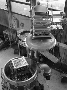
Figure 1: Photographic view of the experimental setup during cosmic ray tests, showing the PMT matrix placed inside the vacuum chamber and the tracker (mwpcs) and trigger (scintillator paddles) system installed on the chamber lid, the latter being moved with a crane.

The prototype consisted of a matrix of 132 3/4” diameter Philips XP2802 photomultiplier tubes (PMT) available from a previous experiment [3]. The size was compatible with the requirements defined from the preliminary simulation results. The PMTs were equipped with a lime glass window allowing photon detection over the wave length range {280-640} nm. The tubes were mounted mechanically with individual magnetic shieldings on a support frame of aluminium drilled with appropriately spaced housing holes. Each PMT was mounted on a socket connected by a short cable to the front end electronics board adjacent to the matrix. The counter was installed in a vacuum chamber equipped with a pumping system for tests in vacuum. Two experimental configurations were used for cosmic ray and beam particle detection respectively.

In the two experimental setups, the prototype was complemented with a set of detectors implemented to define the event, provide a trigger to the DAQ system, and allow the incident particle trajectory reconstruction.

In the cosmic ray configuration, the counter surface was placed horizontally, facing the sky. A simple tracker made of 3 $xy$ multiwire proportionnal chambers (MWPC) 40x40 cm² with 2 mm wire spacing, and equipped with delay line readouts, was placed above the vacuum chamber (see fig.  1). It was used for incident trajectory reconstruction using the three space points provided by the MWPCs. The spatial resolution obtained for the extrapolated trajectory impact on the detection plane was about 1 mm in both directions, a value which did not affect sensitively the accuracy of the Cherenkov event reconstruction. Three plastic scintillator paddles of different sizes read by PMTs, defining the angle of acceptance on the radiator, were interleaved with the MWPCs and used to define the trigger. They also provided dE/dX and time of flight (TOF) informations. Figure 1 shows a photographic view of the setup in cosmic ray configuration.

The beam test configuration is described in section 9. Details on the setup and on the calibration procedures are given in ref [8].

Radiators: Two types of radiator materials considered as suitable for the final counter have been evaluated, as discussed in ref [4].
1) Sodium Fluoride ($N\!aF\,$), a crystal with low refractive index [10]. It was chosen because of its suitability for low momentum particle identification (range $\approx$0.5-4 GeV kinetic energy per nucleon).
2) Silica aerogel (AGL). Several values of the refraction index were investigated because of their suitability for the intermediate and high momentum range of particle identification. One of them was used in the threshold Cherenkov counter ($ATC$) which flew with AMS on the STS 91 shuttle flight [27]. The size and basic properties of the radiators for Cherenkov light emission (mean refraction index $<\!n\!>$ , threshold velocity $\beta_{th}$ and momentum per nucleon (nuclei) $P_{th}$, limiting Cherenkov angle $\theta_{c}^{\infty}$, photon yield, and chromatic dispersion) are given in table 1. The numbers are calculated taking into account the Cherenkov spectral distribution and PMT overall quantum efficiency. $<\!n\!>$ is the mean refractive index of the material used as radiator, $\beta_{c}$($P_{th}$) is the Cherenkov velocity (momentum) threshold. The momentum range $P_{range}$ is defined between the Cherenkov emission threshold and the upper momentum limit defined by 4$\sigma$ separation of one $amu$ mass difference for a 1 cm thick radiator at the chromatic limit (see [4]). $\theta_{c}^{\infty}$ is the limiting Cherenkov angle and $<\!N_{pe}\!>$ is the expected number of photoelectrons to be detected for $Z=1$ particle assuming that the full detection area is sensitive. The experimental results for these radiators are available in Table 2

Both NaF and aerogels are transparent in the useful wave length range considered, extending from the upper UV region (300 nm) up to the (low yield) red region. See discussion below for the aerogels. The two materials combine very conveniently for maximizing the momentum range of particle identification [4].

Table 1: Physical parameters of the radiator materials used in the study as described in the text.

Material	$<\!n\!>$	Size	Thickness	$\beta_{c}$	$P_{range}$	$\theta_{c}^{\infty}$	$<\!N_{pe}\!>$	$\frac{\delta n}{n}$
		(mm)	(cm)		GeV/c/uma	(mrad)	(cm${}^{-1})$	$\times 10^{3}$
NaF	1.33	8.5$\times$8.5	1	0.75	1-6.5	719	28	$\sim 3$
NaF	1.33	8.5$\times$8.5	0.5	0.75		719	28	$\sim 3$
aerogel	1.14	4.1$\times$4.1	0.65	0.877	1.8-8	501	20	$\sim 2$
aerogel	1.05	5$\times$5	2.5	0.952	2.9-10	310	-	-
aerogel	1.035	11$\times$11	1.1	0.966	3.4-11.5	261	6	$\sim 0.5$
aerogel	1.025	11$\times$11	1.1	0.976	4.2-12	221	4	$\sim 0.3$

3 Readout electronics and data acquisition

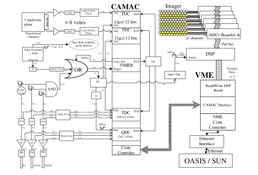
Figure 2: Architecture of the signal processing electronics and data acquisition system used with the prototype. The abreviations stand for: CFD : Constant Fraction Discriminator, AF : Analog Fan-out, LF : Logic Fan-out, D : Amplitude Discriminateur, TDC : Time to digital Converter, QDC : Charge to digital Converter,

The design of the dedicated low power consumption readout electronics developed for this project is described in ref [11]. The readout and packaging system is built in a modular form composed of eight 32 channels processing boards connected to a bus together with a DSP board and a VME interface (dual access memory) for data storage and communication with the data acquisition system. The set up can process 256 channels. In the present case, only 144 channels (6 boards of 24 channels) were used. See ref [12] for the prototype II version currently in test phase (not used here).

A general layout of the electronics setup used in the measurements is shown on fig 2. The trigger to DAQ was obtained by requiring a coincidence between the plastic scintillator paddles.

The data were recorded by means of a general purpose data acquisition system ($DAQ$) allowing the online monitoring of the experiment [13]. Part of the software has been developed by the authors for the purpose of the present study. The data were put on disk and transferred to a data storage facility.

4 Method of analysis

The analysis procedure was built along the following steps. First the geometrical alignments and calibrations required for the various detector were performed as described below. Next, each particle trajectory was first recontructed and then extrapolated onto the photodetector plane, providing the reference point for the Cherenkov pattern reconstruction. The validation cuts were then applied to the data, and for each photon of each event the Cherenkov angle $\theta_{c}$ and the azimuthal angle $\phi_{c}$ were reconstructed individually using the algorithm described in [4]. Next, background photons were removed from the $\theta_{c}$ distribution, and finally the velocity of the particle was calculated using a weighted circular regression fit to the selected pattern, also described below.

The charge Z of the particle was calculated in a separate step, from the total number of Cherenkov photoelectrons measured for the event, by summing the response of the (calibrated) fired PMTs, using a dedicated background rejection procedure, and correcting for: a) The loss of internally reflected photons (NaF radiator only) according to the trajectory angle (see [4]), and b) The loss of refracted photons escaping laterally from the drift space of the counter.

4.1 Detector geometrical alignment

For each run, the reference frame of the tracking system and of the PMT matrix had to be carefully aligned with respect to the photodetector reference frame. Indeed, a misalignment of the two detectors along transverse coordinates, generated a periodic dependence of the reconstructed Cherenkov angle $\theta_{c}$ on the azimuthal photon angle $\phi_{c}$ measured with respect to the projection of the mid-radiator point of the trajectory on the detector plane, and a subsequent double peaking of the reconstructed $\theta_{c}$ distribution. A $\phi_{c}$-independent $\theta_{c}$ distribution can be easily obtained from a small sample of raw events by adjusting the $\Delta X$ and $\Delta Y$ transverse offset of the two coordinate systems. A good enough value of the $\Delta X$ and $\Delta Y$ offsets can be calculated using events with particle interacting with a PMT entrance window on the trajectory (see section 5 for signal characterization). Assuming the PMT $X_{PM}$ and $Y_{PM}$ known geometrical coordinates on the detector plane, one can evaluate straightforwardly:

$$\left\{\begin{array}[]{l}\Delta X=\overline{X_{PM}-X_{track}}\\ \\ \Delta Y=\overline{Y_{PM}-Y_{track}}\end{array}\right.$$

from the overall sample of data. The calculation of the mean is restricted to $|\Delta X|$ and $|\Delta Y|$ smaller than the PMT pitch ($\approx$25 mm). The calculation may require several iterations if the misalignment happens to be of the order of the detector pitch.

4.2 PMT gain and threshold alignments

The PMT sockets were grouped by 4 on a 40 channels High Voltage power supply. The mean gain of the PMTs on the detector was $G=3.4\times 10^{6}$. On each processing board, the collected charge measurement was performed by a dedicated self-triggering analog ASIC micro-circuit ensuring charge to voltage conversion. The output voltage was digitized by a 12 bits analog-to-digital converter (ADC). A dynamic range of 100 has been chosen, based on estimate of the charge measurement range to be covered. This allowed the single photoelectron amplitude (SPE) to be encoded on about 40 channels. The electronic pedestal measurement of each channel was performed during dedicated runs. The PMTs calibration was performed using a blue LED diode. The diode light intensity was first set to a value and then reduced to reach the SPE signal on each channel of the detector. The calibration was then made assuming an exponential shape for the thermal (dynode) noise and a gaussian SPE response. In some cases, when the PMT response was poor, the second and third photoelectron peaks were taken into account [9]. The gain measurement accuracy is estimated to be $\pm$5%. The mean SPE resolution of the tubes was (RMS over mean value): $\frac{\sigma}{q}\approx\,50\pm 14\,\%$, a reasonable result considering that the PMTs used were ageing.

The triggering level of each channel was set to approximately 0.3 SPE signal, so as not to lose SPE hits and to limit (thermal) background hits. It could be recorded directly in the ASIC memory during dedicated runs, the value being $\sim 15-20\,mV$ under $50\,\Omega$, depending on the channel.

4.3 Photon background

The photon background on the imager had to be treated with particular care since for $Z=1$ particles, the yield is small with $\sim$1-10 hit pixels per event, depending on the radiator material, and non-discriminated noise hits could damage considerably the accuracy on the velocity measurement. The mean overall background on the detector has been estimated from the data analysis to be of the order of 1-2 hits per event. Background hits triggering the ASICs can occur from the following sources:

• PMT dark current: This contribution has been investigated by means of a random trigger generator during dedicated runs. The mean dark current (frequency of triggering) per PMT was relatively high with $f\approx 2500$ Hz because the PMTs were enclosed in a metallic black box in which the equilibrium temperature was elevated due to the PMT socket heat dissipation. As the acquisition time of the ASIC is $\tau_{asic}\approx 500$ ns, the probability to have one noise hit on the imager per event due to PMT dark current, could be estimated:

  $$T_{dc}=126\times f\times\tau_{asic}\approx\,15\%$$

• Particle interactions in the PMTs can influence contiguous tubes. Cross-talk effects have been observed by studying samples of events that do not cross the radiator. The probability to have at least one fired PMT on the trajectory was $\approx 75\%$.

• Reflected Cherenkov Stray photons or Rayleigh scattered photons (for AGLs), reflected towards the detection plane. These photons were lost for the velocity measurement, but could be counted for $Z$ measurement. This contribution has not been investigated in details.

5 Data selection

Good events were selected by application of a set of software cuts to the data sample. A good event was defined by requiring valid particle trajectory, particle geometry, and Cherenkov pattern.

• Valid particle trajectory: Three space points from the three MWPCs and a chisquare $\chi^{2}<3$ in the linear regression on the 3 sets of $xy$ hit coordinates of the particle trajectory.

• Valid particle geometry: The extrapolated particle trajectory on the detector plane must cross the radiator.

• Valid Cherenkov pattern:
  At least three valid Cherenkov photon hits, i.e., below the upper limit in amplitude, which depends on the particule charge. The cut on the Cherenkov pattern was processed in two steps. First, large amplitude hits lying around the extrapolated particle trajectory originating either from the Cherenkov yield of particles crossing the PMT entrance windows, or from electrons produced in the crossing of dynodes, were excluded (referred to as the TC cut in the following). It consists of excluding the PMT crossed by the reconstructed trajectory and all the adjacent PMTs ( 7 pixel cut). The second algorithm was applied next to the remaining hit pixels for background hit rejection.

Two methods for Cherenkov cluster identification in the $\theta_{c}$ angle distribution of hits have been tested. Both were applied after a preliminary sorting of the individual reconstructed Cherenkov angles $\theta_{ci}$ by increasing value order. In the first algorithm, a cluster is identified as a set of Cherenkov angles in which the angular distance between any two hit angles is smaller than a fixed value $\delta\theta_{1}$. A clustering weight $w_{i}$ proportional to the number of contiguous hits is associated to each $\theta_{ci}$ angle. The value of the weight of pixel $i$ then informs on its number of adjacent neighbours. For instance, only two adjacent pixels would give a 1-1 sequence in term of cluster weight, while a group of 3 pixels would give 1-2-1. The raw hit multiplicity $\mu$ of an event is separated into two parts so that $\mu=s+n$, where $s$ is the number of hits assigned by the cluster algorithm while $n$ is the sum of the rejected hits. In our study, a Cherenkov cluster is kept if $s\geq 3$ with $s>n$. Hence, a valid cluster contains at least one weight equals to two, which is an easy criterion to check, and the minimal weight pattern is 1-2-1. In a normal run, events with several clusters were rejected. This algorithm has been successfully used to identify two independent Cherenkov patterns in the double radiator configuration described in the section 7.4. The $\delta\theta_{1}$ value has been investigated experimentally. It has been underlined that the $\delta\theta_{1}$ optimum is a compromise between $\chi^{2}$ likelihood (see section 6) and ring reconstruction efficiency $\epsilon$, defined as the ratio of the number of reconstructed rings on the number of events passing the cuts. These two numbers are calculated on the basis of the set of events with a validated reconstructed trajectory. When $\delta\theta_{1}$ is too small, a fraction of good hits is rejected and $\epsilon$ decreases, while for $\delta\theta_{c}$ too large, $\epsilon$ is maximized but the likelihood is poor since noise hits have not been efficiently rejected. For the prototype, the optimum value for NaF was $\delta\theta_{1}\approx 35$ mrad while for 1.035 AGL radiator $\delta\theta_{1}\approx 80$ mrad. This method has given satisfactory results in rejecting noise hits far enough from the Cherenkov cluster as it will be shown further below.

The second method is simpler to compute and consists of assuming the median value $\theta_{cm}$ (of the sorted individual values of $\theta_{c}$) to be always located in the cluster. The valid Cherenkov angles are then those for which $|\theta_{c}-\theta_{cm}|\leq\delta\theta_{2}$. Here the optimum value of $\delta\theta_{2}$ was around $50$ mrad for both Naf and AGL. The two methods give similar results.

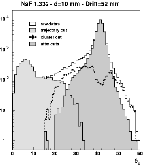
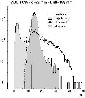
Figure 3: Distributions of individual Cherenkov angles $\theta_{c}$ obtained for: 10 mm NaF radiator with $52$ mm drift space (left), and 22 mm AGL radiator ($n=1.035$) with $189$ mm drift (right). Solid line : raw data; Diamonds: individual $\theta_{c}$ cut by the cluster algorithm; light gray: individual $\theta_{c}$ cut by the TC cut algorithm; Dark Gray: remaining distribution of $\theta_{c}$ after both cuts have been applied.

(a)	(b)
Figure 4: (a) Example of event obtained with a 10 mm thick NaF radiator and a 72 mm drift gap. Full circles are Cherenkov hits (black) and background hits (gray). The particle was an atmospheric muon ($\beta\sim 1$) with too large a velocity to be resolved with the prototype. (b) Distribution of reconstructed $\theta_{c}$ values for this event hits, using the particle track parameters. Three bakground hits are seen neatly separated from the Cherenkov cluster. (c) Circular regression fit for the same event of the Cherenkov ring in the trajectory frame (rejected hits labelled *).
	(c)

Figure 3 illustrates the results for two radiator materials. It shows the raw $\theta_{c}$ distribution (solid line histograms) for NaF radiator (left), and AGL 1.035 radiator (right) for cosmic ray (CR) particles. On both figures, two peaks are seen at low and high $\theta_{c}$ values, the latter close to $\theta_{c}^{\infty}$ value, containing most of good events. The small angle peak is due to particles interacting with PMTs. The specific cut of these low angle hits (TC cut) corresponds to the pale gray histogram. It consists of a peak at small angle riding on a broader distribution extending to higher $\theta_{c}$ values. The peak reflects the angle distribution between the center of the hit pixel and the impact point of the particle on the imager (the $\theta_{c}$ reconstruction algorithm takes the center of the PMT photocathode as photon hit coordinates [4]). On figure 3(a), the peak is observed around 5 ^∘ while the broader structure extends up to 30^∘. This structure is a consequence of the cross-talk effect between the hit PMT and its adjacent neighbours. Cutting these cross talk effects is necessary but has the unwanted drawback of cutting the Cherenkov signal for particles having velocities close to the Cherenkov threshold, since for small $\theta_{c}$ the reconstructed rings is contained within the first circle of PMTs around the particle impact. Thus, on the prototype, the effective $\beta$ threshold is somewhat higher than the $\frac{1}{n}$ value. This effect is expected to be limited however with smaller pixels as it will be in the final design. It will also depend on cross talk between pixels for the PMTs used.

On fig 3, the part of the distribution cut by the cluster algorithm is represented by diamond histograms. The peaking around $\theta_{c}^{\infty}$ is seen to shrink significantly for both radiators, showing the efficiency of the cut. This is particularly clear for the AGL radiator where the high $\theta_{c}$ tail due to Rayleigh scattered photons is reduced by about one order of magnitude. Note that the cusp generated in the distribution for NaF is a small $\approx$1% effect.

The distribution of $\theta_{c}$ remaining after cuts is displayed in dark gray. The large angle tail for AGL can be partly cut out by requiring individual $\theta_{ci}$ to be less than $\theta_{c}^{\infty}+3\delta\theta_{1}$ for instance. For Naf, the shoulder around $30^{\circ}$ is probably physical since the hit multiplicity observed for these events is consistently decreasing with $\theta_{c}$ as expected for Cherenkov photons.

An example of CR event measured with NaF radiator is displayed on figure 4(a), with the matrix of PMT array represented. The arrow shows the projection on the detector plane of the particle trajectory between the entry point in the upper MWPC and the intercept on the detector plane (arrow head). The reconstructed individual $\theta_{c}$’s for this event are shown on figure 4(b). The Cherenkov cluster is easily identified to the peak on the right, close to $\theta_{c}^{\infty}$. The noise hit at $\approx 6^{\circ}$ is removed by the TC cut. The other two background hits are rejected by the cluster algorithm.

6 Particle velocity reconstruction

On the detection plane, the Cherenkov pattern generated by refraction of the photons at the radiator exit interface is a complexe curve. A simple circular regression fit procedure can be used however by transforming the hit coordinates to the trajectory frame where the Cherenkov light is uniformly distributed on a cone, and the hits along a circle. The individual azimuthal angles $\phi_{c}$ defined below in the detector frame, can be expressed to give new azimutal $\psi_{c}$ angles in the trajectory frame. The parametric equations of the circle are given by (per unit of length) :

$$\left\{\begin{array}[]{l}x=\tan\theta_{c}\cos\psi_{c}\\ \\ y=\tan\theta_{c}\sin\psi_{c}\\ \end{array}\right.$$

The free parameter of the fit appears to be the reconstructed radii: $r_{i}=\tan\theta_{c}{{}_{i}}$, and the $\chi^{2}$ function becomes:

$$\chi^{2}=\sum_{i=1}^{N}\frac{\left(r_{i}^{2}-r^{2}\right)^{2}}{\sigma_{r^{2}_{i}}^{2}}$$

The uncertainty $\sigma_{r^{2}_{i}}$ on $r_{i}^{2}$ is calculated numerically pixel by pixel, for any incident particle angle. $\sigma_{r^{2}_{i}}$ includes contributions from the hit pixel multiplicity, its size and position according to the particle trajectory, radiator thickness, trajectory uncertainty, radiator chromatism, and multiple scattering of particle in the radiator. A dedicated analytical approach of these quantities has been developed in reference [8]. See also [3] for the circular regression technique. The ring radius $r_{c}$ minimizing the $\chi^{2}$ function is then :

$$r_{c}^{2}=\frac{\sum_{i=1}^{N}\frac{r_{i}^{2}}{\sigma_{r^{2}_{i}}^{2}}}{\sum_{i=1}^{N}\frac{1}{\sigma_{r^{2}_{i}}^{2}}}$$

from which the experimental velocity $\beta$ can be derived:

$$\beta=\frac{1}{n}\sqrt{1+r_{c}^{2}}$$

An example of reconstructed velocity with $\chi^{2}$ minimization is available on figure 4(c). It is the last step of the event reconstruction process illustrated on figure 4(a).

7 Measurements with cosmic ray particles

The average count rate was of the order of 0.2 s^-1. A typical run duration was one to three days, providing on the average 17000 events per day.

radiator	$<\!n\!>$	$d$	$D$	$\epsilon$	$\epsilon^{*}$	$\frac{\delta\beta}{\beta}$	$N_{pe}$	$N_{pix}$
		[mm]	[mm]	[%]	[%]	$\times 10^{3}$
NaF	1.332	10	52	$91\pm 4.1$	$>91$	8.8	19.5	7.7
AGL	1.14	13	110	$60.8\pm 2.3$	$>60.8$	9.0	7.2	4.2
AGL	1.05	25	220	$>80\pm 2.5$	$>85.1$	4.7	8.2	5.8
AGL	1.035	22	189	$58.1\pm 2.5$	62.4	4.3	4.8	3.4
AGL	1.035	33	245	$67.0\pm 2.1$	71.3	3.5	7.1	4.7
AGL	1.025	23	321.8	$51.8\pm 1.7$	58.3	2.7	4.9	3.0
AGL	1.025	34.5	310.3	$65.1\pm 1.9$	73.2	2.8	6.6	4.0
AGL	1.025	46	298.8	$66.1\pm 2.2$	74.4	2.7	7.3	4.3

Table 2: List of radiators studied in CR tests. Here, $<\!n\!>$ is the mean refraction index of the radiator over the spectral range of the PMTs for Cherenkov light, $d$ is the radiator thickness, $D$ the drift gap, $\epsilon$ the ratio of the reconstructed event number over trigger number, $\epsilon^{*}$ the reconstruction efficiency corrected from the cosmic ray spectrum below Cherenkov threshold, i.e., triggering scintillators but producing no Cherenkov light for particles down to $\beta=0.88$ [16]. $\frac{\delta\beta}{\beta}$ is the velocity resolution obtained from a gaussian fit around $\beta=1$. $N_{pe}$ and $N_{pix}$ are the mean number of photons and the mean number of firing pixels per event after cuts, respectively.

7.1 NaF radiator

The mean refraction index calculated taking into account the Cherenkov light energy distribution and the quantum efficiency of the PMT photocathode is $<\!n\!>=1.332$. This material has been successfully used previously in the CAPRICE balloon experiment [15]. The maximum Cherenkov angle is $\theta_{c}^{\infty}\approx 41^{\circ}$. The refraction outside the radiator increases this angle to $\approx 61^{\circ}$ for particles normal to the detector plane. In practice, this value limited the drift distance usable on the prototype to a small range around $4-5$ cm for the full ring to be contained in the detector surface.

A good reconstruction efficiency of about $90\%$ was obtained for CRs with this radiator because of its high light yield and good transparency (see table 2). The mean multiplicity was $7.7$ after cuts for 1 cm thick radiator. The best velocity resolution achieved with the NaF was $\frac{\delta\beta}{\beta}=8.8\times 10^{-3}$. This rather poor value is mainly due to the small drift distance mentionned above which, combined with the large pixel size (1.8 cm) lead to a large uncertainty on the ring radius measurement. The large chromatic dispersion for this radiator lead to a contribution of the same magnitude as the former contributions to the overall uncertainty on the velocity measurement [4]. For large incidence angles, a significant fraction of the ring is internally reflected inside the radiator and is lost for detection. This effect however, is not expected to deteriorate the velocity resolution [2, 4].

7.2 Aerogel radiators

Several Silica Aerogel (AGL) samples have been tested in the prototype with the refraction index values $n=1.14,1.05,1.035$ and $1.025$. This type of radiator allows to fill part of the gap in the range of usable refraction index between gas and solid radiators. They became widely studied and used recently [18, 19, 20, 21, 22, 23, 24] because of their low refraction index and chromatism compared to cristals (roughly a factor ten smaller), these quantities being correlated, see appendix and [4, 25] for details. One drawback of AGLs is the Rayleigh scattering phenomenon due to the microscopic structure of the material. Photons are scattered inside the radiator material, and loose their angular coherence. The scattering cross section is larger for short wave lengths [18], and scattered photons generate a wide background halo around the unperturbed Cherenkov ring. AGLs however are currently the only available material to cover certain range of refraction index and then of particle velocity (see [4] for details). The results on the velocity resolution and the experimental photoelectron yield for AGLs are summarized in table 2, where it is seen that the velocity resolution globally improves with the decreasing refraction index (and correlated chromatic dispersion), as it can be expected from general considerations [4, 8]. The velocity resolution can be expressed in terms of chromatism and of the uncertainty on the $\theta_{c}$ measurement per photon, from the Cherenkov relation $\cos\theta_{c}=\frac{1}{\beta n}$ :

$$\frac{\delta\beta}{\beta}=\frac{\delta n}{n}+\tan\theta_{c}\,\delta\theta_{c}$$

$\delta\theta_{c}$ being the experimental uncertainty on the $\theta_{c}$ measurement. It is clear from this well known relation that the velocity resolution improves with the decreasing chromatic dispersion provided the uncertainty on $\theta_{c}$ is kept smaller than the latter.

A velocity resolution $\frac{\delta\beta}{\beta}=9\times 10^{-3}$ could be obtained with the AGL 1.14 sample. Although the sample was apparently of rather poor optical quality, the results are close to the chromatic limit (see discussion in section 4.1). The AGL 1.05 sample [26] provided a significantly better value, $\frac{\delta\beta}{\beta}=4.7\times 10^{-3}$, and the best reconstruction efficiency of the AGL sample tested, probably in account of the good transparency of this sample. The AGL 1.035 sample used [26] was part of the spare tiles from the Aerogel Threshold Counter built for the AMS01 experiment [27]. The measurements provided a value of the resolution $\frac{\delta\beta}{\beta}=3.5\times 10^{-3}$, with a reconstruction efficiency however, decreasing down to around $70$% for a 3 cm radiator thickness, with respect to the AGL 1.05 sample, due to the lesser clarity of this material than for the 1.05 index. The AGL 1.025 sample [26] provided the best velocity resolution obtained in the tests, $\frac{\delta\beta}{\beta}=2.7\times 10^{-3}$. Several runs made with increasing radiator thickness showed that above $\approx 3$ cm, both the reconstruction efficiency (for Z=1 particles) and the velocity resolution remained approximately constant around $70$ % and $2.7\times 10^{-3}$ respectively. This was expected since, when the radiator thickness increases, the net gain of non-scattered Cherenkov photons drops rapidly (+1.7 SPE between 2 and 3 cm, and only +0.9 between 3 and 4).

It can be observed in table 2 that for aerogels the achieved resolution scales with (n-1)/n as expected for the chromatic limit [4]. However the contributions to the resolution in all cases of the table are dominated by the pixel size contribution. The latter nevertheless follows closely the value of the chromatic contribution, generating the observed effect.

7.3 Stability of the long term Cherenkov light yield of silica aerogel

Figure 5: Ratio of the hit multiplicity distribution to the number of triggers, measured for the three runs of january and november 1999, and january 2001, as discussed in the text. One run is not shown for the legibility of the figure.

The rapid decrease in time of the Cherenkov yield of the AGL in the ATC counter observed in the AMS01 experiment [27] has been a major concern for the AMS collaboration, the stability in time of the Cherenkov response of AGL becoming an issue. It was pointed out in a previous note [28] that the ATC AGL tiles have been processed and conditionned with chemically active products like solvants and wave length shifter, and that a chemical contamination was more likely than an (unoticed so far) ageing phenomenon of Silica. Although the observed effect is still awaiting for a proven explanation, the issue has been addressed experimentally with the study prototype and the Cherenkov yield of the AGL monitored over about two years (January 1999 to january 2001). During this time, 4 runs have been recorded in identical conditions, using an AGL 1.035 sample from the AMS01 spares, by 6 months intervals of time, providing hit multiplicity distributions shown on figure 5. Unfortunately, the prototype has been accidentally exposed for several hours to attenuated day light before the third run (june 2000) was taken, resulting in a significant decrease of the overall PMT detection efficiency by about 30%. However, runs on NaF were measured after each AGL runs, and the AGL/NaF ratio of the Cherenkov yield was the same within a small statistical uncertainty before and after the accident, thereby providing a mean to normalize the late runs with respect to the early ones (table 3). As seen on figure 5, the results are unambiguous: No significant decrease of the mean multiplicity could be observed, and no evidence could be obtained for a natural ageing process of the material. The results are summarized in table 3. See [28] for other details and a discussion of the origin of the decaying light yield observed for the ATC counter in AMS01.

Table 3: Fraction of reconstructed events for the 4 runs measured in the same conditions with the RICH study prototype and n=1.035 aerogel (two tiles 1 cm thick superimposed) over a two year period of time. The second and third columns give the ratio of reconstructed events (above threshold) over valid triggers (trajectories) and the associated statistical uncertainties in percent, respectively. Note that this is not the reconstruction efficiency since valid triggers include particles below the Cherenkov threshold ($\approx$4 GeV/c). The fourth column shows the $NaF/AGL$ counting ratio for the four runs, while the last column gives the mean value of the $AGL$ hit multiplicity distributions shown on figure 5. The yields for the last two runs have been normalized to the $NaF$ values. The uncorrected values are given in parenthesis (see text).

Date of data	Reconst. evts	Error	Ratio	Mean hit
	% of triggers	$\sigma$	$NaF/AGL$	multiplicity
Jan 1999	56.6	1.7	0.571	6.31
Nov 1999	55.5	2.3	0.556	6.55
Jul 2000	40.6	1.4	0.532	6.27 (5.72)
Jan 2001	43.4	1.6	0.543	6.41 (5.84)

7.4 Dual radiator configuration

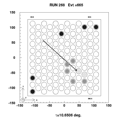
Figure 6: Example of double ring event obtained with the dual radiator setup. $\tau$ is the incident particle angle on the radiator.

The interest of using a dual radiator system lies in the extension of the momentum range covered by the counter for a single radiator. In the present case, the idea was to combine NaF and AGL materials, in order to reach a broad identification range over the full counter fiducial area, allowing identification of ions from the NaF threshold at 480 Mev kinetic energy per nucleon, up to the upper limit for AGL 1.025, between 13 and 20 GeV/n for ions with mass about A=25 and A=4 atomic units respectively [4]. This broad range of sensitivity was dictated by considerations on the Physics case for the AMS RICH [6]. Since the Cherenkov angles are very different for the two media, the risk of confusion is minimized, and the only difficulty to overcome was to find the appropriate way of processing the double hit-pattern.

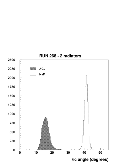
Figure 7: Distribution of the reconstructed Cherenkov angles for the double radiator run, with AGL 1.035 (hatched histogram) and NaF (solid line). See text for details.

Figure 8: Double $\beta$ measurement obtained in the dual radiator run. From top to bottom : $\beta$ measurement with NaF, AGL, and mean of the two measurements.

A dedicated CR run was performed with the prototype, combining a 5 mm thick NaF and a 22 mm thick AGL (1.035) put together in a stack, to investigate the feasability of reconstructing simultaneously the two Cherenkov patterns. The AGL tile was placed above and the total drift distance between the NaF tile and the matrix was 110 mm. This configuration is a compromise, rather far from the individual optimum geometry for the two radiators: for this drift distance, the ring size of the NaF photon pattern is of the order of the matrix size, while for the AGL photons it is of the order of the pixel size. Hence, a number of NaF photons is expected to be lost out of the detector, while the small AGL pattern is very closed to the lower limit of reconstruction imposed by the TC cuts (see section 5). This problem however should vanish with the smaller pixel size and large detector area of the final counter.

The double pattern reconstruction used in the analysis was based on the same cluster algorithm as developped in section 5, with some modifications. First, the events were processed assuming all the photons to be produced in the upper (NaF) radiator. Next, The TC cut was applied, as for a normal single radiator event processing to reject particle-impact related low $\theta$ angles. The following step remained unchanged : the remaining angles were sorted and processed by the cluster algorithm. While in a normal single radiator run, events with more than one cluster were rejected, in the double radiator, double cluster structures were selected as valid events. Since the number of lighted pixels was small, the first type of double structure accepted was $1-1-1-1$ (since one single cluster including all hits would be $1-2-2-1$, see section 5), which means only two pixels fired for NaF and two for AGL. The small $\theta_{c}$ cluster was assumed to be AGL. On this basis, the AGL $\theta_{c}$ angles were calculated taking into account the refraction in the NaF tile. An example of double ring identification is displayed in figure 6. The level of gray represents the result of the cuts. The dark pixels are accepted NaF photons. The medium gray pixels are accepted AGL photons, while the light gray pixels have been rejected as background. The events were then validated after the following condition on the consistency of the velocity measurements was fulfilled :

$$\frac{\beta_{NAF}-\beta_{AGL}}{\frac{1}{2}(\beta_{NAF}+\beta_{AGL})}\leq 5\,\sigma_{\beta_{NAF}}\approx 0.05$$

The distributions obtained from the analysis of this double $\theta_{c}$ measurement are displayed in figure 7. The dark hatched histogram located around $\theta_{c}=15^{\circ}$ is the AGL photon distribution, while NaF photon angles are standing as expected around $\theta_{c}=41^{\circ}$. The AGL $\theta_{c}$ distribution is distorted due to the small ring size (of the order of the pixel pitch) that generates a double peaking distribution, depending on the position of passage of the particle on the detector (see section 9.1). This effect was also observed for beam tests with NaF for low $\beta$ ions (small ring size). The upper tail of the AGL distribution, also visible in figure 3(a), is a consequence of Rayleigh scattering in this radiator.

Figure 8 shows the result of the double $\beta$ measurement in the momentum range above the AGL threshold. It is seen that the velocity measurement on the bottom histogram with $\sigma_{\beta}\approx\sigma_{\beta\,NAF}\oplus\sigma_{\beta\,AGL}$ is slightly improved with respect to the individual measurements. The mean $\beta$ value slightly larger than one comes from the inaccuracy on the mechanical setting of the drift distance which ultimately translates into the observed overestimate.

7.5 Albedo particle rejection

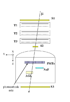
Figure 9: Schematic view of the experimental setup used for the Albedo tests.

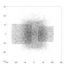
Figure 10: Distribution of reconsructed CR track intercepts on the radiator plane for particles producing one hit or more on the detector (see text).

Particles can enter the AMS spectrometer detector either from the top or from the bottom (Albedo particles). Since a particle entering from the bottom fakes an antiparticle entering from the top, it is clear that, disregarding the rejection power provided by the other AMS detectors, the capability of the RICH to discriminate these two types of events, must be evaluated. Albedo particles are not expected to generate a response from the counter. However, some Cherenkov light is produced, and then can be detected, and good events can be faked by unfortunate combinations of random hits. This issue has been adressed experimentally with the prototype. The results of the study have been reported in [14]. They are summarized here for convenience.

In the Albedo CR configuration, the prototype was set upside down, the photocathodes facing the ground. CRs entering from the top are thus equivalent to albedo particles for the RICH in orbit. Two radiators were tested in a single run: $10\mbox{mm}$ NaF, d=70 mm, and $3\times 11\mbox{mm}$ AGL, d=157 mm. they were arranged as shown on figure 9.

Albedo data were taken with CRs for 14 days. The analysis showed that some Cherenkov photons could reach the imager from both radiators. Figure 10 shows the distribution of the CR track intersections with the radiator planes, with the minimal condition of at least 1 hit on the detector required. The profiles of the NaF and AGL radiator tiles are clearly seen on the right and left of the figure, respectively. The rectangular shape visible at the center is an image of the global counter acceptance to CRs. It was generated by the fired PMT located on the track. This photon yield can generate events with multiplicity$>$1 that could fake Cherenkov patterns. Among 22209 Albedo NaF events, 11 went through all cuts, whereas none of the 27104 AGL events could make it (see table 4). This difference is an acceptance effect : $\beta=1$ rings from AGL are smaller than those from NaF. Therefore fake rings have a larger probability to occur with NaF than with AGL.

The results could be well accounted for assuming that background hits are randomly distributed on the imager [14]. This successful interpretation enables us to estimate the rejection power for Albedo particles in the AMS RICH. For the NaF radiator, it is estimated to be $R\sim 10^{4}$ when requiring 3 hit minimum in the Cherenkov cluster. Requiring a larger multiplicity improves the rejection efficiency, each extra unit enhancing the rejection power by a factor $\approx 50$. For the same requirements, the rejection power obtained with the AGL 1.025 radiator is very good $R\approx 10^{6}$. However, Albedo particles have momenta typically $P\lesssim 5$ GeV/c per nucleon, and the threshold of this radiator $P\approx 4.1$ GeV/c/nuleon , is of marginal interest for the rejection purpose.
Therefore, the RICH could contribute efficiently to the Albedo particle rejection.

Radiator	NaF	AGL
Drift distance [mm]	70.2	157.4
$R_{c}$ [mm]	130	51
Statistics	22209	27104
Through cuts	11	0
Rejection power	2019	$>27104$
Probability	$4.95\times 10^{-4}$	$<3.68.10^{-5}$

Table 4: Experimental results for the Albedo particle detection for the two radiators. $R_{c}$ is the ring radius expected for $\beta=1$ particles. Statistics is the whole number of events with a valid reconstructed trajectory falling in the acceptance of the detector array. Through cuts is the number of events that faked a Cherenkov ring (see text). The Rejection Power is the ratio of the full counting statistics over the number of validated events passing the cuts. Probability is the inverse of the Rejection power that gives the probability to mistake an albedo particle as a normal particle in the RICH.

8 Monte Carlo simulation

(a)	(b)

Figure 11: Comparison of the simulation results (dashed lines) with the experimental data for cosmic rays (muons, solid line) for AGL radiator $n=1.025$ (a) and NaF radiator (b).

The experimental CR data have been compared to simulation results performed with an adapted version of the code used in the first simulation study of the RICH [4], using the same event reconstruction procedure. No background contribution was included in this simulation.

The muon flux at ground level was described as in [16]. The small proton flux ($\approx$10% of muon flux) was included and the electron flux was neglected ([17]). The relevant PMT characteristics were taken into account : collection efficiency of first dynode assumed to be $0.9$, quantum efficiency of photocathode according to the technical datasheet of the manufacturer, SPE resolution taken the same for all PMTs as the mean value from calibration measurements (see section 4.2). The uncertainty on the reconstruced coordinate of the particle hit in the mid plane of the radiator was modelised by a gaussian of $2$ $\sigma$ in both X and Y direction, the value of $\sigma$ including both spatial resolution of the MWPCs and multiple scattering in the radiator.

The result for the NaF radiator is in good agreement with the experimental CR data (see table 5 and figure 11(b)). The velocity resolution is reproduced to within a few %, as well as the hit pixel multiplicity. This point is important since it validates the predictions of the simulation program. The origin of this good agreement is mainly due to the fact that the optical properties of the radiator are very well known (chromatism, transparency…).

The AGL radiator light yield were less straightforward to modelize because their optical properties were not as well known as for NaF, and because of the secondary effects in the light transmission (absorption and Rayleigh scattering). The AGL clarity coefficients $C\approx 10^{-2}$ $\mu$ m ⁴ cm ^-1 [26] were available from the manufacturer for the n$<$1.05 samples. The AGL chromatic dispersion used was based on the scaling law $\frac{\delta(n-1)}{n-1}=cte$ using the measured values of silica (see appendix and [4]). This approximation has been recently shown to be in excellent agreement with the data [25]. The results obtained however, are not good as seen in table 5 and figure 11(a), since the simulated resolution is significantly better than measured, although the simulated hit pixel multiplicity is in reasonable agreement with the data. No satisfactory explanation has been found for this discrepancy.

radiator	$\langle n\rangle$	$d$	$D$	$\frac{\delta\beta}{\beta}\times 10^{3}$		$N_{pix}$
		[mm]	[mm]	sim.	exp.	sim.	exp.
NaF	1.332	10	52	8.9	8.8	7.5	7.7
AGL	1.14	13	119	3.6	7.9	5.4	4.2
AGL	1.05	25	220	2.7	4.7	5.3	5.8
AGL	1.035	33	245	2.1	3.5	6.5	4.7
AGL	1.025	34.5	310.3	1.9	2.8	4.4	4.0

Table 5: Comparison of the experimental CR results with simulation. $\langle n\rangle$ is the mean refraction index of the radiator, $d$ the radiator thickness, $D$ the drift distance, and ${(\frac{\delta\beta}{\beta})}$ the velocity resolution from the simulation (sim) and measured at $\beta\sim 1$ (exp), $N_{pix}$ being the number of fired pixels after cuts.

9 Measurements with beam particles

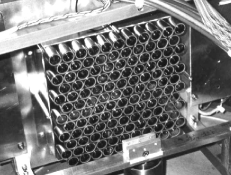
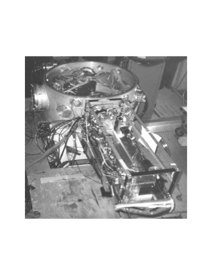
Figure 12: Closeup view of the PMT matrix (top) and general view of the setup used at GSI, showing the prototype in the vacuum chamber and the tracking and triggering detectors upstream.

The prototype has been tested at the GSI/Darmstadt ion accelerator facility with ${}^{12}C$ beams with incident energies of 0.6, 0.8, 1, 1.2, and 1.4 Gev/nucleon.

In the test beam configuration, the detection plane was set vertical in the vacuum chamber, facing beam particles. The detector was placed on a movable arm around the fixed radiator holder. The radiator was placed at the center of the chamber and kept parallel to the detector surface, i.e., the two were rotating together, so that mesurements for different incident particle angles on the radiator could be achieved easily. The radiator could also be placed further upstream if necessary. The incident beam particle angles on the radiator could be varied between 0 and 45 deg. Two small MWPCs placed upstream of the chamber were used to define the incident trajectory, and a set of three small area (typically $10\times 10$ cm²) scintillators framing the MWPCs along the beam line, provided the event trigger. The beam MWPCs were mainly used for providing the transverse coordinate of the particle hit on the detector matrix, for event reconstruction. Pictures of the matrix and setup on the beam line are shown on figure 12.

Only the NaF radiator could be tested in this experiment since the maximum beam velocity of the accelerator was below the Cherenkov threshold for the aerogel materials considered (see table 1). The same NaF tiles were used as for the cosmic ray measurements.

Beam particles with different masses were obtained by placing a fragmentation target (a beam monitoring quartz was used to this purpose) upstream of the magnetic dipole analyzer. Fragments with atomic mass from 1 to 12 could then be obtained, with momenta defined by the field setting of the analyser. For a given beam energy, the various fragment mass and momenta could be obtain with a few bins of rigidity. With this method a set of data on nuclei over a range of mass and charge could be obtained to test the response of the prototype for each incident energy. Very low beam intensities were used, typically well below 10³ particles.s^-1, with very low angular divergence $<\theta>\approx 1$ mrd, and a size about 1x1 cm² at the target. Higher intensities could be used when fragments with A/Z different from the incident beam value were selected, the primary beam particles being off the detector area. The measurements were performed during a three days run on April 1998. Figure 14 shows an example of Cherenkov ring for a helium particle.

9.1 Effects of the photodetector dead area

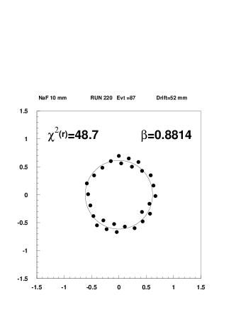
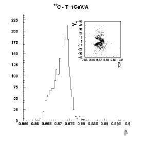
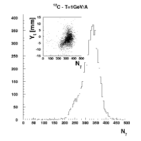
Figure 13: Fit on the Cherenkov ring produced by a Helium ion, reconstructed in the reference frame of the trajectory.

Figure 14: Distribution of reconstructed $\beta$ values (left) and number of photoelectrons $N_{\gamma}$ (right) for ${}^{12}C$ beam particles at $T=1$ GeV/A. The inserts show the evolution of $\beta$ and $N_{\gamma}$ respectively, as a fonction of the Y coordinate of the center of the reconstructed ring on the imager.

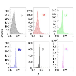
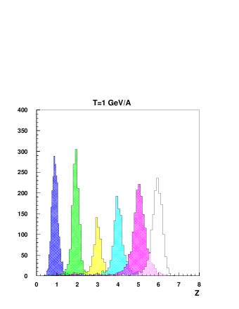
Figure 15: Experimental velocity $\beta$ obtained with $T=1~{}GeV/A$ ${12}$C beam fragments obtained as described in the text. The elements were identified separately by means of the redundant of dE/dX measurement provided by the trigger scintillator counters [8]. The Z=6 incident beam particle spectrum was been taken from a separate run.

Figure 16: Experimental Z reconstruction obtained with $T=1~{}GeV/A$ ${12}$C beam fragments in the same conditions as in figure 16.

The active area (packing fraction) of the photodetector was about 56% of the total surface. This dead area had a very regular pattern which particular geometry generated some distortion effects in the event reconsruction. The main reason holds to the (radial) ring width and pattern cell dimension of the dead area being of the same order of magnitude. In this case, the overlap between the Cherenkov ring and the active detector area depends on the ring position on the imager. This effect induces a systematic error which has been observed experimentally during beam tests. It generates a tail at low values in the distribution of the number of detected photoelectrons (figure 14(a)), and in the $\beta$ distribution (figure 14(b)).

This systematic error has been investigated and can be very well reproduced with a simple model [8]. It is also reproduced with the simulation program. It can be corrected for by means of a simple algorithm which provides good results for the charge reconstruction. The correction on $\beta$ is more difficult to implement since the ring width depends on $\beta$ and is lower than the pixel size. Pixel size and packing fraction of the final imager however will largely exclude this effect.

9.2 Particle velocity and charge reconstruction

The data sample analyzed for $\beta$ and Z reconstruction included only normal incident particles, with Cherenkov rings fully contained inside the detector area, then with no acceptance correction necessary.

The final particle velocity reconstruction is illustrated on figure 16. The $\beta$ resolution was observed to improve with the increasing $Z$ of the particle, as expected from the Cherenkov radiation law. The agreement with the expected $Z$ dependence according to the relation:

$$[\frac{\delta\beta}{\beta}]_{Z}=\frac{1}{Z}[\frac{\delta\beta}{\beta}]_{Z=1}\;,$$

was fair to within the experimental uncertainties [4] as seen in table 6. Indeed, it can be seen that the quantity $Z[\frac{\delta\beta}{\beta}]_{{}_{Z}}$ is approximately constant, the larger excursion from the expected value for $Z$=1 and 2 being mainly due to the distorsion effect quoted in the previous section.

The particle charge reconstruction was based on the $Z$ dependence of the Cherenkov photon yield:

$$N_{\gamma}\propto\,Z^{2}\sin^{2}\theta_{c}$$

The Z separation depends practically (although it should not theoretically [4]) on the photon yield. It was typically 15 $PE$ for $\beta=0.85$ protons. The hit rejection cuts used for this reconstruction were softer than for the $\beta$ reconstruction, in order to avoid rejecting good hits. Only those hits located on the reconstructed trajectory were discarded. The effect on the $Z$ resolution would be significant with an AGL radiator because of Rayleigh scattering of Cherenkov photons. It is small however for a NaF radiator. Table 6 summarizes the results and the Z distribution histogram obtained is shown on figure 16. The light ions with $Z\leq 3$ are well separated with $\frac{\Delta Z}{\sigma_{Z}}\approx 5$. For heavier ions however, the separation degrades down to $3-4$ for $Z=3,4,5$. This effect seems to be due to the onset of a saturation of both the PMTs above $\approx 20$ PE per pixel and (some of) the ADC electronics, in account of the high PMT gain used. This effect should disappear with smaller pixel size PMTs, as it is foreseen for the AMS RICH.

element	$\beta$	$\frac{\delta\beta}{\beta}\times 10^{3}$	$N_{pix.}$	$N_{\gamma}$	$\sigma_{\gamma}$	$Z$	$\sigma_{Z}$	$\frac{\Delta Z}{\sigma_{Z}}$
p	0.85	10.8	7.75	14.8	7.5	0.9	0.15
He	0.864	8.7	15.8	65.2	17.2	1.9	0.17	5.9
Li	.875	4.1	21.5	177.8	28.5	3.0	0.19	5.2
Be	.882	3.3	27.0	342.9	40.6	4.0	0.24	4.2
B	.885	2.8	31.6	551.3	70.6	5.0	0.28	3.6
C	.873	2.4	28	701	56.8	5.95	0.24	4.2

Table 6: Reconstructed $\beta$ and $Z$ values for a $T=1$ GeV/A particle beam with normal incidence on the radiator. $N_{pix}$ is the mean hit pixel multiplicity, $N_{\gamma}$ the mean number of $PE$, $\sigma_{\gamma}$ the RMS of this latter distribution, $Z$ the reconstructed charge and $\sigma_{Z}$ the RMS of the Z distribution. $\frac{\Delta Z}{\sigma_{Z}}$ is the separation between two consecutive charges in RMS units (i.e., $\frac{1}{\sigma_{Z}}$).

10 Summary and conclusion

The study of a first generation prototype of proximity focussing RICH counter for the AMS experiment reported in this paper has allowed an end-to-end investigation of the technique: Instrumental test of the detector components and electronics, test of the reconstruction and background rejection algorithm, background measurement, and finally measurement of the counter resolution with different radiator samples using both incident cosmic rays and beam ions with Z$<$6, casting the grounds of the future AMS RICH counter.

The above work is being followed by a second generation prototype which incorporates the main features and elements of the final RICH design (flight model). It will be operated using the same instrumental peripheral environment as in the present work. This phase is being undertaken in collaboration between all the institutions involved in the effort on the RICH project .

Acknowledgements.
The authors are very indebted to R .Simon for his invaluable help during the data taking at GSI. They are extremely grateful to M. Yokoyama (Matsushita), J. Favier (LAPP Annecy) and P. Fisher (MIT), for providing aerogel samples, and to B. Ille (IPN Lyon) for making the set of MWPCs available to the authors. They are also indebted to R. Blanc, T. Cabanel, G. Gimon and M. Marton for their contribution to the detector assembly, to A. Garrigue, F. Vezzu, and E. Perbet, for their contribution to the mechanical study, to J. Bouvier and O. Rossetto for their help in the setting up of the electronics, and to Z. Ren for his help on the detector simulation.
One of the authors (A.M-R.) wishes to acknowledge the ISN hospitality and partial support of CONACYT and DGAPA-UNAM.
This work was made possible by a dedicated grant from the IN2P3/CNRS.

Appendix: Refractive index and Cherenkov radiator thickness

This appendix briefly addresses the issue of the physical variables governing the refractive index and chromatic dispersion of materials. The implication on the thickness of the Cherenkov radiators is discussed.

The relationship between the refractive index and the phsical of a medium is governed by the Lorentz-Lorenz (L-L) law, which can be expressed as [29]:

$$\frac{n^{2}-1}{n^{2}+2}={\cal N}\alpha(\lambda)$$ (1)

In this relation, $n$ is the refractive index of the material, $\cal N$ the number density of particles in the medium, and $\alpha(\lambda)$ the dipole polarizability of the molecules of the medium, i.e., their response function to electromagnetic driving forces.

For small values of $(n-1)$ it is straightforward to see that the above can be written as:

$${n-1}\approx\frac{3}{2}{\cal N}\alpha(\lambda)$$ (2)

Since ${\cal N}$ can be expressed in terms of the mass density $\rho$ of the medium ($\rho={\cal\frac{N}{V}A})$, with ${\cal A}$ the molar mass of the material, and $\cal V$ the Avogadro number), one has the relation of proportionality:

$${n-1}\approx\rho\alpha(\lambda)$$ (3)

This simplified form of the L-L equation puts in evidence a few important properties of the refractive index of (transparent) materials:
1) - The quantity $(n-1)$ scales with the density $\rho$ of the material. Therefore, $(n-1)$ will change by approximately 3 orders of magnitude between the gas phase (under atmospheric pressure) and the solid phase for a given element.
2) - The dependence of $(n-1)$ on the wave length $\lambda$ of the incident light is governed by the response function of the molecules of the medium to the corresponding electromagnetic perturbation. The relative variation of $(n-1)$ over a given range of $\lambda$ is thus given by the relative variation of the molecular response function $\alpha$:

$$\frac{\Delta(n-1)}{n-1}\approx\frac{\Delta\alpha}{\alpha}$$ (4)

Therefore, the scaling law $\frac{\Delta(n-1)}{n-1}\approx constant$ holds rather strictly to within the validity of the approximation for a given material.

The derivative of equation 1 can be evaluated rigorously however, leading to:

$$\frac{2n}{(n^{2}+2)(n+1)}\frac{\Delta(n-1)}{n-1}=\frac{\Delta\alpha}{\alpha}$$ (5)

The evaluation of the term multiplying the quantity $\frac{\Delta(n-1)}{n-1}$ in this relation can be verified to be about constant, close to 0.3 for values of n between 1 and 1.5. The approximation

$$\frac{\Delta(n-1)}{n-1}\approx constant$$ (6)

is then basically correct, although it is more accurate to use relation 5.

3) - It is important to note that the chromatic dispersion of ($n-1$) also scales with the matter density, i.e.:

$$\Delta(n-1)\approx\rho\Delta\alpha(\lambda)$$ (7)

$\Delta\alpha(\lambda)$ being taken over some relevant range of $\lambda$. This explains in general why the chromatism of low density materials, like gas or aerogels, is much smaller than that of high density materials like crystals. This explains in particular why it is so for aerogels compared to quartz or fused silica, and it provides a way of estimating the chromatism of the former from the known dispersion law of the latter.

Thickness of Radiator material
The above discussion has straightforward implications for the thickness of the radiator material to be used for a RICH counter. This thickness can be expressed in terms of the Cherenkov variables. The number of photons radiated is N_ph=N₀Lsin${}^{2}\theta$, where N₀ is the quality factor of the counter [4], L the radiator thickness, and $\theta$ the Cherenkov angle. One has therefore $L=\frac{N_{ph}}{N_{0}sin^{2}\theta}$, or $L\approx\frac{N_{ph}}{2N_{0}<n-1>}$ for small values of $(n-1)$. Using relation 3 above: $L\approx\frac{N_{ph}}{2N_{0}\rho<\alpha>}$, or

$$\rho L=\frac{N_{ph}}{2N_{0}<\alpha>}$$ (8)

The quantity $\rho L$ is the thickness of the radiator in g/cm². It is seen that this quantity is constant for a given number of photons and for a given material. Although the quality factor can be somewhat different however for different values of $n$, this effect is small for refractive index not too much different, like between 1.02 and 1.1 in silica aerogels. With this restriction, relation 8 shows that the thickness of material to be used for a given number of photoelectrons does not depend on the mean refractive index of the material with the same molecular structure. For different materials the relation does not hold since the asymptotic value of $\alpha(\lambda)$ depends on the value of the first pole of the dispersion law [29], which can differ by an order of magnitude from one material to another.

References

- [1] J. Litt and R. Meunier, Ann. Rev. Nucl. Sci. 23(1973)1;
- [2] J. Séguinot and T. Ypsilantis, Nucl. Inst. and Meth. in Phys. A343(1994)30
- [3] J. Ballon et al., Nucl. Inst. and Meth. in Phys. A338(1994)310
- [4] M. Buénerd and Z. Ren, Nucl. Inst. and Meth. in Phys. A454(2000)476
- [5] S. Ahlen et al., Nucl. Inst. and Meth. in Phys., A350(1994)351; S.C.C Ting, Phys. Rep. 279(1997)203
- [6] A. Bouchet et al., Nucl. Phys. A688(2000)417c;
- [7] Z. Ren et al., Nucl. Instrum. Meth. in Phys. A433(1999)172; T. Thuillier et al. Nucl. Instrum. Meth. in Phys. A 461(2001)278
- [8] T. Thuillier, Thesis, Institut des Sciences Nucléaires, Université J. Fourier, Grenoble, May 15, 2000, report ISN 00-47.
- [9] E.H. Bellamy et al., Nucl. Inst. and Meth. in Phys., A339(1994)468
- [10] P. Carlson et al., Nucl. Inst. and Meth. in Phys., A349(1994)577
- [11] L. Gallin-Martel, J. Pouxe, O. Rossetto, and P. Stassi, Nucl. Inst. and Meth. in Phys. A 433(1999)444; L. Gallin-Martel, J. Pouxe, and O. Rossetto, Proc of the IEEE conf, Toronto, November 1998, report ISN/97-26, Grenoble, April 1997.
- [12] L. Gallin-Martel, J. Pouxe, and O. Rossetto, A new front end electronics for the AMS RICH, ISN Grenoble report ISN/99-30, April 1999, eprint physics/9812018
- [13] R. Duet, N. Borrome, H. Harrock, T. Tran-Kahn, P. Didelon and J. Navarre, OASIS Data Acquisition system, Internal report, IPN Orsay, 1994; D. Barancourt, G. Barbier and B. Meillon, ISN Grenoble, private communication.
- [14] T. Thuillier et al., Nucl. Inst. and Meth. in Phys. A461(2000)278
- [15] P. Carlson et al.,Nucl. Inst. and Meth. in Phys. A349(1994)577
- [16] O.C. Allkofer, P.K.F. Grieder, Cosmic Rays on Earth, Physics Data, ISSN 0344-8401.
- [17] Review of Particle Physics, Eur. Phys. J., C15(2000)150
- [18] D.E. Fields et al., Nucl. Inst. and Meth. in Phys., A349(1994)431
- [19] R. De Leo et al., Nucl. Inst. and Meth. in Phys., A401(1997)187
- [20] Y. Asaoka et al., Nucl. Inst. and Meth. in Phys., A416(1998)236
- [21] A. Gougas et al., Nucl. Inst. and Meth. in Phys., A421(1999)249
- [22] E. Aschenauer et al., Nucl. Inst. and Meth. in Phys., A440(2000)338
- [23] R. De Leo et al., Nucl. Inst. and Meth. in Phys., A457(2001)52
- [24] E. Nappi, Aerogel and its applications to RICH detectors, Conf. on advanced technology in particle physics, Como 96, Nucl. Phys. B., 61B(1998)270
- [25] M.F. Villoro et al., Nucl. Instrum. Meth. in Phys. A, in press
- [26] Matsushita Electric Works Ltd, Osaka, Japan
- [27] D. Barancourt et al., Nucl. Instrum. Meth. in Phys. A 465(2001)306
- [28] M. Buénerd ans T. Thuillier, AMS Note 99-11-04 and ISN Grenoble report 99-122. See also, J. Favier, R. Kossakovski and J.P. Vialle, AMS note 2001-03-05
- [29] M. Born and A. Wolf, Principle of Optics, Pergamon, 1975.