Stationary state in N-body System with power law interaction

Abstract

Many self-gravitating systems often show scaling properties in their mass density, system size, velocities and so on. In order to clarify the origin of these scaling properties, we consider the stationary state of N-body system with inverse power law interaction. As a simple case, we consider the self-similar stationary solution in the collisionless Boltzmann equation with power law potential and investigate its stability in terms of a linear symplectic perturbation. The stable scaling solutions obtained are characterized by the power index of the potential and the virial ratio of the initial state. It is suggested in general that the nonextensive system has much various stable scaling solutions than those in the extensive system.

I introduction

There are many self-gravitating systems which are characterized by some scaling properties. For example, the inter stellar medium shows that its velocity dispersion $\sigma$ is power law related with the system size $L$ or mass $M$larson81 ($\sigma\sim L^{0.38}\sim M^{0.2}$) and isothermal contour is characterized by the fractal dimension $D\sim 1.36$falgarone91 . The observations by the Hubble Space Telescope show elliptical galaxies have a power law density distribution $\rho\sim r^{-n}$ (at outer region, $n\sim 4$ and at inner region, $n\sim 0.5-1.0$ for the bright elliptical galaxies and $n\sim 2$ for the faint onesmerritt96 .). The distribution of the galaxies and the cluster of galaxies can be characterized by the fractal dimension $D\sim 2$pietronero . In cosmological simulations based on the standard cold dark matter scenario, the density profile shows a power law distribution (at outer region, $n\sim 3$ and at inner region, $n\sim 1.0-1.5$NFW97 ; makino01 .).

Recently, in order to study the statistical properties of a self-gravitating system, we proposed the self-gravitating ring modelsota , where all particles are moving, on a circular ring located in three-dimensional space, with mutual interaction of gravity in three-dimensional space. The numerical simulation shows that the system at the intermediate energy scale, where the specific heat becomes negative, has some peculiar properties such as non-Gaussian and power law velocity distribution($f(v)\sim v^{-2}$), scaling mass distribution, and self-similar recurrent motion. In this model, the halo particles which belong to the intermediate energy scale are considered to play an important role in realizing such specific characters.

We are interested in the origin of these scaling properties from statistical mechanical point of view. In order to study the statistical properties of long range interaction such as gravity, Ising model, and spin glass, the model with power law potential has been used and revealed anomalous propertiesIspolatov2001 ; Campa2001 ; Campa2002 . For example, a gravitational-like phase transitionIspolatov2001 , reduction of mixingCampa2001 , and long relaxationCampa2002 are observed. Using a model with an attractive $1/r^{\alpha}$ potential in general D-dimensional space, we can control the extensivity of the system and the specific heat by changing the spatial dimension $D$ and the exponent of inverse power of the potential $\alpha$.

In this paper, we study the quasi-equilibrium state of N-body system with a power law potential. As a first step, we consider the collisionless Boltzmann equation (CBE) in place of N-body system and derive the self-similar stationary solution of CBE which has a scaling property appearing in the quasi-equilibrium state and discuss the linear stability by the use of energy functional analysiskandrup90 ; kandrup91 ; perez96 ; Rey96 .

In section II, we show some general properties of N-body systems with power law potential. In section III, we derive the self-similar stationary solution of CBE with an attractive $1/r^{\alpha}$ potential assuming spherical symmetry and isotropic orbit case in D-dimensional space. Stability for the linear perturbation around the self-similar stationary solution is investigated in section IV. Section V is devoted to discussion.

II N-body system with power law potential

In this section, we show some general characteristic properties of N-body system with power law potential.

We write the Hamiltonian for the N-body system with power law potential in the form:

$$H=\sum_{i=1}^{N}\frac{P_{i}^{2}}{2m}-\sum_{i<j}^{N}\frac{Gm^{2}}{r_{ij}^{\alpha}},$$ (1)

where $r_{ij}:=|r_{i}-r_{j}|$ and $\alpha$ controls the range of interaction.

In this system, the virial equilibrium condition becomes

$$2<K>+\alpha<\Phi>=0,$$ (2)

where $<K>$ is the time averaged kinetic energy and $<\Phi>$ is the time averaged potential energy. From the expression $H=K+\Phi$, we have

$$H=-\frac{2-\alpha}{\alpha}<K>=\frac{2-\alpha}{2}<\Phi>.$$ (3)

From Eq.(3), the signature of the specific heat is determined by the signature of the term $-(2-\alpha)/\alpha$.

In order to clarify the extensivity / nonextensivity of the system, we focus on the $N$ dependence of the potential energy $\Phi$ under fixing the number density $N/L^{D}$Tsallis95 :

$$\frac{\Phi}{N}\sim\int^{N^{(1/D)}}drr^{D-1}r^{-\alpha}\sim N^{1-\alpha/D}.$$ (4)

If the $N$ dependence of the potential energy per particle disappears for $N\rightarrow\infty$. we define the system extensive. Otherwise, we define the system nonextensive. In the case of the gravity in $D$-dimensional space, since $\alpha=D-2$, the system is always nonextensive. We summarize the signature of the specific heat of the system and the extensivity in Table.1.

Table 1: In the system with an attractive $1/r^{\alpha}$ potential in $D$-dimensional space, the property of the specific heat and the extensivity is shown.

	$0<\alpha<2$	$\alpha>2$
specific heat	negative	positive
	$\alpha<D$	$\alpha>D$
extensivity	nonextensive	extensive

III Self-Similar stationary solution in Collisionless Boltzmann Equation (CBE)

In this section, we derive a self-similar stationary solution in the collisionless Boltzmann equation (CBE);

$$\frac{df}{dt}=\frac{\partial f}{\partial t}+[f,H]=0.$$ (5)

where $f=f(\bm{x},\bm{v},t)$ is a mass distribution function and $[A,B]$ denotes the Poisson bracket.

The stationary solution $f_{0}$ satisfies the following equation,

$$[f_{0},H]=\sum_{i=1}^{2D}\frac{\partial w^{i}}{\partial t}\frac{\partial f_{0}}{\partial w^{i}}=0,$$ (6)

where $w^{i}=\{\bm{x},\bm{v}\}$.

For the coupled CBE and Poisson equation, R.N. Henriksen and L.M. WidrowSSS studied the self-similar stationary solution in CBE with spherical symmetry in three-dimensional space by applying the systematic method which is based on the work of B. Carter and R.N. HenriksenSS .

Following R.N. Henriksen and L.M. WidrowSSS , we study the self-similar stationary solution with spherical symmetry and isotropic orbit case in general D-dimensional space. The case that $D=3$ and $\alpha=1$ reduces to the work by R.N. Henriksen and L.M. WidrowSSS . By the generalization of the spatial dimension $D$ and the exponent of power of potential $\alpha$, we intend to investigate the relation between the extensivity of the system and the self-similarity.

From Eq.(6), mass distribution function $f(r,v)$ obeys

$$v\partial_{r}f-\partial_{r}\Phi\partial_{v}f=0,$$ (7)

where $v:=\sqrt{v_{r}^{2}+v_{\theta}^{2}+v_{\phi}^{2}}$ and $\Phi$ is a potential. The potential $\Phi$ satisfies the following equation,

$$\frac{1}{r^{D-1}}\partial_{r}\left(r^{\alpha+1}\partial_{r}\Phi\right)=S_{D}^{2}G\int v^{D-1}fdv,$$ (8)

where $S_{D}:=2\pi^{D/2}/\Gamma(D/2)$. In the case of $\alpha=D-2$, the above equation corresponds to Poisson equation.

A self-similar stationary solution satisfies the following equation,

$${\cal L}_{\bm{k}}f=0,$$ (9)

where

$${\cal L}_{\bm{k}}:=k^{i}\partial_{i}=\delta r\partial_{r}+\nu v\partial_{v}+\mu m\partial_{m}$$ (10)

is a Lie derivative with respect to the vector $\bm{k}$ in phase space, and $\delta$, $\nu$, and $\mu$ are arbitrary constants.

In a dimensional space of length, velocity, and mass, we introduce vectors ${\bm{a}}=(\delta,\nu,\mu)$ and ${\bm{d}}_{f}$. The vector ${\bm{a}}=(\delta,\nu,\mu)$ describes changes in the logarithms of dimensional quantities. Each dimensional quantity $f$ in the problem has its dimension represented by the vector ${\bm{d}}_{f}$. Using these vectors ${\bm{a}}$ and ${\bm{d}}_{f}$, the action of ${\bm{k}}$ reads

$${\cal L}_{\bm{k}}f=({\bm{d}}_{f}\cdot{\bm{a}})f.$$ (11)

The dimensional quantities in current problem $f$, $\Phi$, and $G$ have the following dimensional covectors,

$${\bm{d}}_{f} = (-D,-D,1),$$

$${\bm{d}}_{\Phi} = (0,2,0),$$ (12)

$${\bm{d}}_{G} = (\alpha,2,-1).$$

The requirement of the invariance of $G$ under the rescaling group action (10) implies ${\bm{d}}_{G}\cdot{\bm{a}}=0$,

$$\mu=\alpha\delta+2\nu.$$ (13)

The dimensional space is reduced to the subspace of (length, velocity), wherein the rescaling group element ${\bm{a}}=(\delta,\nu)$ and

$${\bm{d}}_{f} = (\alpha-D,2-D),$$

$${\bm{d}}_{\Phi} = (0,2).$$ (14)

Here we define the new coordinate $R(r)$ and $X$ in replacement of the original coordinate $r$ and $v$ such that

$${\cal L}_{\bm{k}}R=1,$$ (15)

$${\cal L}_{\bm{k}}X=0.$$ (16)

From Eqs.(15) and (16), we choose

$$r|\delta| = e^{\delta R},$$ (17)

$$v = Xe^{\nu R}.$$ (18)

The transformation from the original coordinate $(r,v)$ to the self-similar coordinate $(R,X)$ is shown in AppendixA.

Under the new coordinate, these physical quantities $f$ and $\Phi$ can be written in the form:

$$f(X,R) = \overline{f}(X)e^{-[(D-\alpha)\delta+(D-2)\nu]R},$$ (19)

$$\Phi(X,R) = \overline{\Phi}(X)e^{2\nu R}.$$ (20)

Substituting Eqs.(19) and (20) into Eqs.(7) and (8), these equations for a bounded solution yield

$$\!\!\!\!\!\!\!\!\!\!\!\!\frac{d\ln\overline{f}}{d\ln X}=-\frac{\left[D-2+(D-\alpha)\frac{\delta}{\nu}\right]X^{2}}{X^{2}+2\overline{\Phi}},$$ (21)

$$\!\!\!\!\!\!\!\!\!\!\!\!2\nu^{2}|\delta|^{D-\alpha-2}\left[2+\frac{\alpha\delta}{\nu}\right]\overline{\Phi}=S_{D}^{2}G\int_{0}^{\sqrt{-2\overline{\Phi}}}\!\!\!\!\!\!\!\!X^{D-1}\overline{f}dX.$$ (22)

Without loss of generality, we can set $\nu=1$.

Solving Eqs.(21) and (22), we have the following solution,

$$\overline{f}=C|X^{2}+2\overline{\Phi}|^{-[(D-\alpha)\delta+(D-2)]/2},$$ (23)

where

$$C=\frac{\left|2+\alpha\delta\right||\delta|^{D-\alpha-2}\Gamma(D/2)\Gamma(2+(\alpha-D)\delta/2)}{2\pi^{D}G|-2\overline{\Phi}|^{(\alpha-D)\delta/2}\Gamma([4-D+(\alpha-D)\delta-D]/2)},$$

(24)

and the following condition must be satisfied,

$$(D-\alpha)\delta<4-D.$$ (25)

Since $\overline{\Phi}<0$, from Eq.(22) we obtain the additional condition,

$$\alpha\delta<-2.$$ (26)

If these condition Eqs.(25) and (26) are actually satisfied, we have the bounded self-similar stationary solution (23) and (24). The mass distribution function $f$, the mass density $\rho$, and the velocity distribution $f(v)$ become respectively

$$f(r,v) = C|2E|^{-[(D-\alpha)\delta+(D-2)]/2},$$ (27)

$$\rho := S_{D}\int dvv^{D-1}f(r,v)\sim r^{\alpha-D+2/\delta},$$ (28)

$$f(v) := S_{D}\int drr^{D-1}f(r,v)\sim v^{\alpha\delta+2-D},$$ (29)

where $E$ denotes the mean field energy:

$$E:=\frac{1}{2}v^{2}+\Phi_{0}.$$ (30)

The ratio of the average of the kinetic energy to the potential energy is as follows:

$$\frac{<\Phi_{0}>}{<K>} = \frac{(D-\alpha)\delta-4}{2D}.$$ (31)

Since the solution (27) we obtained is a bounded solution, which satisfies the following condition,

$$\frac{(D-\alpha)\delta-4}{2D} < -1,$$ (32)

the specific heat of the self-similar stationary solution is always negative. The $\delta_{*}$ corresponds to a virial equilibrium state:

$$\delta_{*} = \left\{\begin{array}[]{@{\,}ll}-\frac{4}{\alpha}&(\alpha\neq D)\\ \mbox{arbitrary}&(\alpha=D).\end{array}\right.$$ (35)

If $(D-\alpha)(\delta-\delta_{*})<0$, the potential energy in this state is more dominant than in the virialized state.

The relation between pressure $P$ and mass density $\rho$ can be written in the form:

$$P\sim\rho^{1+\frac{1}{1+(\alpha-D)\delta/2}}.$$ (36)

The above equation of state corresponds to Polytropes gas when identifying the Polytropes index $n$ as $1+(\alpha-D)\delta/2$. Note that for $\alpha=D$, there is no self-similar stationary solution corresponding to the isothermal state.

As for gravity case ($\alpha=D-2$), the above solution (24) and (27) in $D=3$ corresponds to the solution derived by R.N. Henriksen and L.M. WidrowSSS . For $D=1$ and $D=2$ where $\alpha=D-2\leq 0$, we show the self-similar stationary solution in Appendix B.

IV Linear perturbation analysis

In this section, we investigate the stability of the self-similar stationary solution derived in the previous section for a symplectic linear perturbation, by energy functional analysiskandrup90 ; kandrup91 ; perez96 ; Rey96 .

As for the linear stability of the stationary solution in CBE of the gravity in three-dimensional space, there has been much research BT87 ; antonov61 ; antonov62 ; lyndenbell69 ; ipser74 ; sygnet84 ; bartholomew71 ; kandrup90 ; kandrup91 ; perez96 ; Rey96 . For the stationary state, assuming spherical symmetry, characterized by the mass distribution function $f_{0}$ specified as a function of the mean field energy $E$ and the squared angular momentum $J^{2}$, if $\partial f_{0}/\partial E<0$ and $\partial f_{0}/\partial J^{2}<0$, then the system is stable to the linear perturbation.

Following the work by J. Perez and J.J. Alyperez96 where the stability of stationary solution in the coupled CBE and Poisson equation with spherical symmetry in three-dimensional space was studied, we study the stability of the solution obtained in the previous section.

First, we explain a symplectic linear perturbation by energy functional analysiskandrup90 ; kandrup91 ; perez96 ; Rey96 . In term of the mass distribution function $f(\bm{x},\bm{v},t)$, the Hamiltonian $H$ is written as follows,

$$H=\int d\Gamma\frac{\bm{v}^{2}}{2}f(\bm{x},\bm{v},t)$$

$$+\frac{G}{2}\int\!d\Gamma\!\int\!d\Gamma^{\prime}\!{\cal G}(|\bm{x}-\bm{x}^{\prime}|)f(\bm{x},\bm{v},t)f(\bm{x}^{\prime},\bm{v}^{\prime},t),$$ (37)

where $d\Gamma:=d^{D}\bm{x}d^{D}\bm{v}$ is the $2D$-dimensional phase volume element and the kernel ${\cal G}$ satisfies

$$\Phi(\bm{x})=G\int d\Gamma^{\prime}{\cal G}(|\bm{x}-\bm{x}^{\prime}|)f(\bm{x}^{\prime},\bm{v}^{\prime},t).$$ (38)

We consider a small perturbation around the stationary solution $f_{0}$. The distribution function and Hamiltonian can be expanded around the stationary solution as follows,

$$f(\bm{x},\bm{v},t) = f_{0}+\delta^{(1)}f+\delta^{(2)}f+\cdots,$$ (39)

$$H = H_{0}+\delta^{(1)}H+\delta^{(2)}H+\cdots.$$ (40)

Here we consider any symplectic perturbation, which can be generated from the stationary solution $f_{0}$ by use of a canonical transformation. By using some generating function $K$, any symplectic deformation can be expressed in the form:

$$f=e^{[K,\cdot]}f_{0}.$$ (41)

From the above definition (41), $f$ can also be expressed as follows,

$$f= f_{0}+[K,f_{0}]+\frac{1}{2!}[K,[K,f_{0}]]$$ (42)

$$+\frac{1}{3!}[K,[K,[K,f_{0}]]+\cdots.$$

Introducing a small parameter $\epsilon$ which represents the amplitude of the perturbation, we expand the generating function $K$ as

$$K=\epsilon K^{(1)}+\epsilon^{2}K^{(2)}+\epsilon^{3}K^{(3)}+\cdots.$$ (43)

Further identifying $g^{(n)}=\epsilon^{n}K^{(n)}$, we obtain the perturbed quantities in the Eq.(39) in the form:

$$\delta^{(1)}f = [g^{(1)},f_{0}],$$ (44)

$$\delta^{(2)}f = [g^{(2)},f_{0}]+\frac{1}{2}[g^{(1)},[g^{(1)},f_{0}]].$$ (45)

The first order term in Eq.(40) becomes

$$\delta^{(1)}H=\int d\Gamma E[g^{(1)},f_{0}],$$ (46)

where $E$ is the energy of a particle,

$$E:=\frac{\bm{v}^{2}}{2}+\Phi_{0},$$ (47)

where $\Phi_{0}$ is the potential energy generated by $f_{0}$. Since $E$ and $f_{0}$ are conserved quantities, $\delta^{(1)}H=0.$

The next order term in Eq.(40) yields

$$\delta^{(2)}H=\int d\Gamma E[g^{(2)},f_{0}]+\frac{1}{2}\int d\Gamma E[g^{(1)},[g^{(1)},f_{0}]]$$

$$+\frac{G}{2}\int d\Gamma\int d\Gamma^{\prime}{\cal G}(|\bm{x}-\bm{x^{\prime}}|)[g^{(1)},f_{0}][{g^{(1)}}^{\prime},f_{0}^{\prime}].$$ (48)

The first term in Eq.(48) also vanishes and by the integration by parts, Eq.(48) is rewritten in the form:

$$\delta^{(2)}H=-\frac{1}{2}\int d\Gamma[g^{(1)},f_{0}][g^{(1)},E]$$

$$+\frac{G}{2}\int d\Gamma\int d\Gamma^{\prime}{\cal G}(|\bm{x}-\bm{x^{\prime}}|)[g^{(1)},f_{0}][{g^{(1)}}^{\prime},f_{0}^{\prime}].$$ (49)

Hereafter we consider the case that the stationary solution $f_{0}$ is a function of only the energy $E$. In this case, we obtain

$$[g^{(1)},f_{0}] = F_{E}[g^{(1)},E],$$ (50)

$$\int d^{D}\bm{v}[g^{(1)},f_{0}] = \int d^{D}\bm{v}\partial_{\bm{x}}(F_{E}\bm{v}g^{(1)}),$$ (51)

where $F_{E}:=\partial_{E}f_{0}$.

Integrating by parts and using Eqs.(50) and (51), we have

$$\delta^{(2)}H=$$

$$\frac{1}{2}\int d\Gamma(-F_{E})|[g^{(1)},E]|^{2}+\frac{G}{2}\int d\Gamma\partial_{\bm{x}}(-F_{E}\bm{v}g^{(1)})$$

$$\times\int d\Gamma^{\prime}\partial_{\bm{x^{\prime}}}(-F^{\prime}_{E}\bm{v}^{\prime}{g^{(1)}}^{\prime}){\cal G}(|\bm{x}-\bm{x}^{\prime}|).$$ (52)

The linear perturbation $g^{(1)}$ has two kinds of gauge mode. $(a)$ $g^{(1)}=g^{(1)}(E)$. In this case, the linear perturbation of the mass distribution $\delta^{(1)}f$ is trivially zero. $(b)$ $g^{(1)}=\bm{a}\bm{v}$ ($\bm{a}$ is a constant.). This perturbation means the translation of the center of mass. In order to consider the physical perturbation, we investigate the linear perturbation excluding the above gauge modes.

The stability for the linear perturbationbartholomew71 ; holm reads:

If $$\delta^{(2)}H>0$$, then the system is stable. (53)

IV.1 spherical mode

Since the first order perturbed potential $\delta^{(1)}\Phi(r)$ satisfies

$$\frac{1}{r^{D-1}}\partial_{r}\left(r^{\alpha+1}\partial_{r}\delta^{(1)}\Phi(r)\right)=S_{D}G\int d^{D}\bm{v}^{\prime}[{g^{(1)}}^{\prime},f_{0}^{\prime}]$$

$$=S_{D}G\frac{1}{r^{D-1}}\partial_{r}\left(r^{D-1}\int d^{D}\bm{v}^{\prime}F_{E}^{\prime}v^{r^{\prime}}{g^{(1)}}^{\prime}\right),$$ (54)

the spatial derivative of $\delta^{(1)}\Phi(r)$ becomes

$$\partial_{r}\delta^{(1)}\Phi(r)=\frac{S_{D}G}{r^{\alpha-D+2}}\int d^{D}\bm{v}^{\prime}F_{E}^{\prime}v^{r^{\prime}}{g^{(1)}}^{\prime}.$$ (55)

From Eqs.(52) and (55), we have

$$2\delta^{(2)}H$$

$$=\int d\Gamma(-F_{E})|[g^{(1)},E]|^{2}$$

$$-\int d\Gamma\partial_{r}(-F_{E}v^{r}g^{(1)})\delta^{(1)}\Phi(r)$$

$$=\int d\Gamma(-F_{E})|[g^{(1)},E]|^{2}-S_{D}G\int\frac{d^{D}\bm{x}}{r^{\alpha-D+2}}$$

$$\times\int d^{D}\bm{v}(-F_{E}vg^{(1)})\int d^{D}\bm{v}^{\prime}(-F_{E}^{\prime}v^{r^{\prime}}{g^{(1)}}^{\prime}).$$ (56)

Introducing new variables,

$$g^{(1)}=:rv^{r}\mu(r,\bm{v},t),$$ (57)

and using Schwartz’s inequality, we have

$$2\delta^{(2)}H = \int d\Gamma(-F_{E})|[\mu rv^{r},E]|^{2}-GS_{D}\int\frac{d^{D}\bm{x}}{r^{\alpha-D+2}}$$

$$\times\int d^{D}\bm{v}[-F_{E}r(v^{r})^{2}\mu]\int d^{D}\bm{v^{\prime}}[-F^{\prime}_{E}r(v^{{}^{\prime}r})^{2}\mu^{\prime}]$$

$$\geq \int d\Gamma(-F_{E})|[\mu rv^{r},E]|^{2}-GS_{D}\int\frac{d^{D}\bm{x}}{r^{\alpha-D+2}}$$

$$\times\int d^{D}\bm{v}[-F_{E}r(v^{r})^{2}\mu^{2}]\int d^{D}\bm{v^{\prime}}[-F^{\prime}_{E}r(v^{{}^{\prime}r})^{2}]$$

$$= \int d\Gamma(-F_{E})\left\{|[\mu rv^{r},E]|^{2}-\frac{GS_{D}(rv^{r})^{2}\mu^{2}\rho_{0}}{r^{\alpha-D+2}}\right\},$$

where $\rho_{0}$ is non-perturbed mass density:

$$\rho_{0}:=\int d^{D}\bm{v}f_{0}=\int d^{D}\bm{v}(-F_{E})(v^{r})^{2}.$$ (59)

Using the property of the Poisson bracket, and the fact that the integral of the Poisson bracket over the phase space vanishes, the equation (LABEL:SD-h2) can be rewritten in the form:

$$2\delta^{(2)}H \geq \int d\Gamma(-F_{E})\left\{|[\mu rv^{r},E]|^{2}-\frac{GS_{D}(rv^{r})^{2}\mu^{2}\rho_{0}}{r^{\alpha-D+2}}\right\}$$ (60)

$$= \int d\Gamma(-F_{E})\left\{(rv^{r})^{2}|[\mu,E]|^{2}+|\mu|^{2}|[rv^{r},E]|^{2}\right.$$

$$\left.+rv^{r}[\mu^{2},E][rv^{r},E]-\frac{GS_{D}(rv^{r})^{2}\mu^{2}\rho_{0}}{r^{\alpha-D+2}}\right\}$$

$$= \int d\Gamma(-F_{E})\left\{(rv^{r})^{2}|[\mu,E]|^{2}+|\mu|^{2}|[rv^{r},E]|^{2}\right.$$

$$+[\mu^{2}rv^{r}[rv^{r},E],E]-|\mu|^{2}rv^{r}[[rv^{r},E],E]$$

$$\left.-|\mu|^{2}|[rv^{r},E]|^{2}-\frac{GS_{D}(rv^{r})^{2}\mu^{2}\rho_{0}}{r^{\alpha-D+2}}\right\}$$

$$= \int d\Gamma(-F_{E})\left\{(rv^{r})^{2}|[\mu,E]|^{2}\right.$$

$$\left.-|\mu|^{2}rv^{r}[[rv^{r},E],E]-\frac{GS_{D}(rv^{r})^{2}\mu^{2}\rho_{0}}{r^{\alpha-D+2}}\right\}.$$

Using the following relation,

$$[[rv^{r},E],E] = -rv^{r}\left(\frac{d^{2}\Phi_{0}}{dr^{2}}+\frac{3}{r}\frac{d\Phi_{0}}{dr}\right)$$ (61)

$$= -rv^{r}\left(\frac{GS_{D}\rho_{0}}{r^{\alpha-D+2}}+\frac{2-\alpha}{r}\frac{d\Phi_{0}}{dr}\right),$$

we obtain the final expression in the form:

$$\delta^{(2)}H\geq$$

$$\frac{1}{2}\int d\Gamma(-F_{E})(rv^{r})^{2}\left(|[\mu,E]|^{2}+|\mu|^{2}\frac{2-\alpha}{r}\frac{d\Phi_{0}}{dr}\right).$$

(62)

From Eqs.(44), (49), and (62), if $\delta^{(2)}H=0$ when $F_{E}<0$ and $\alpha\leq 2$, $\delta^{(1)}f=0$. Since this is a gauge mode, we conclude that

If $$F_{E}<0 \alpha\leq 2 \delta^{(2)}H>0$$ and , then . (63)

From the self-similar stationary solution Eq.(23), we have

$$F_{E}=\mbox{sgn}(E)[(\alpha-D)\delta+2-D]C|2E|^{[(\alpha-D)\delta-D]/2}.$$ (64)

As an explicit example, we consider $D=1$ case. From Eqs.(25), (26), (32), and (63), if the following condition is satisfied, the self-similar stationary solution Eq.(27) is stable.

$$-\frac{1}{\alpha-1}<\delta<-\frac{2}{\alpha} 1<\alpha\leq 2$$ ()

$$\delta<-\frac{2}{\alpha} 0<\alpha\leq 1$$ () (65)

In Fig.1, we show the region where exits the stable self-similar stationary solution in the parameter space $(\alpha,\delta)$.

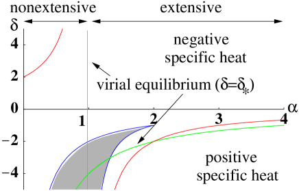
Figure 1: Stability chart for the one-dimensional case ($D=1$). The dark region corresponds to the stable region (65) in the parameter space ($\delta$, $\alpha$). The property of the specific heat and the extensivity also are shown.

Note that in the above calculation, we use the integration by parts and neglect the surface term at the origin. Since the self-similar stationary solution obtained in this paper is singular at the boundary, the surface term can not be neglected in general. In the realistic situation, however, the self-similarity appears in the intermediate scale since the system has a cut off scale in the short distance. We suppose that the self-similar stationary solution can be connected with some regular solution near the boundary by regularization such as $r\rightarrow(r^{2}+a^{2})^{1/2}$ where $a$ is a cut off scale, and the boundary term can be neglected.

IV.2 aspherical mode

Next, we consider the aspherical mode. Since it is difficult to analyze a general case, we study the gravity case in D-dimensional space ($\alpha=D-2$).

By the integral of Poisson equation over the configuration space and integration by parts, we have

$$-\frac{1}{S_{D}}\int d^{D}\bm{x}|\nabla\delta^{(1)}\Phi|^{2}=\int d\Gamma\delta^{(1)}f\delta^{(1)}\Phi,$$ (66)

where

$$\delta^{(1)}\Phi:=\int d^{D}\bm{v}{\cal G}\delta^{(1)}f.$$ (67)

From Eqs.(49), (66), and (67), we have

$$\delta^{(2)}H=\frac{1}{2}\int d\Gamma\frac{(\delta^{(1)}f)^{2}}{-F_{E}}-\frac{G}{2S_{D}}\int d^{D}\bm{x}|\nabla\delta^{(1)}\Phi|^{2}.$$ (68)

Here we introduce $\delta^{(1)}\tilde{f}$ as follows,

$$\delta^{(1)}f=:F_{E}\delta^{(1)}\Phi+\delta^{(1)}\tilde{f}.$$ (69)

Substituting Eq.(69) into Eq.(68), we obtain

$$\delta^{(2)}H$$

$$=\frac{1}{2}\int d\Gamma\left[\frac{(\delta^{(1)}\tilde{f})^{2}}{-F_{E}}+F_{E}(\delta^{(1)}\Phi)^{2}-2\delta^{(1)}f\delta^{(1)}\Phi\right]$$

$$-\frac{G}{2S_{D}}\int d^{D}\bm{x}|\nabla\delta^{(1)}\Phi|^{2},$$

$$=\frac{1}{2}\int d\Gamma\frac{(\delta^{(1)}\tilde{f})^{2}}{-F_{E}}+\frac{1}{2S_{D}}\int d^{D}\bm{x}\biggl{\{}|\nabla\delta^{(1)}\Phi|^{2}$$

$$-S_{D}\left[\int d^{D}\bm{v}(-F_{E})|\delta^{(1)}\Phi|^{2}\right]\biggr{\}}.$$ (70)

Moreover, using the new variable $w$ which is defined by

$$\delta^{(1)}\Phi=:w(\bm{x},t)\partial_{r}\Phi_{0},$$ (71)

we can rewrite the equation (70) in the form:

$$\delta^{(2)}H$$

$$=\frac{1}{2}\int d\Gamma\frac{(\delta^{(1)}\tilde{f})^{2}}{-F_{E}}$$

$$+\frac{1}{2S_{D}}\int d^{D}\bm{x}\Biggl{\{}(\partial_{r}\Phi_{0})^{2}\left[|\nabla w|^{2}-S_{D}\int d^{D}\bm{v}(-F_{E})|w|^{2}\right]$$

$$-|w|^{2}\partial_{r}\Phi_{0}\nabla^{2}\partial_{r}\Phi_{0}\Biggr{\}}.$$ (72)

By straightforward calculation, we obtain

$$\nabla^{2}\partial_{r}\Phi_{0}=S_{D}\int d^{D}\bm{v}F_{E}\partial_{r}\Phi_{0}+(D-1)\frac{\partial_{r}\Phi_{0}}{r^{2}}.$$ (73)

By using Wirtinger’s inequality, we have

$$\int\left[|\nabla_{s}w|^{2}-\frac{D-1}{r^{2}}|w|^{2}\right]d\Omega\geq 0,$$ (74)

where $\nabla_{s}:=\nabla-\frac{\bm{r}}{|\bm{r}|}\frac{\partial}{\partial r}$.

From Eqs.(72), (73), and (74), we get the final expression in the form:

$$\delta^{(2)}H$$

$$=\frac{1}{2}\int d\Gamma\frac{(\delta^{(1)}\tilde{f})^{2}}{-F_{E}}$$

$$+\frac{1}{2S_{D}}\int d^{D}\bm{x}(\partial_{r}\Phi_{0})^{2}\left[|\partial_{r}w|^{2}+|\nabla_{s}w|^{2}-\frac{D-1}{r^{2}}|w|^{2}\right]$$

$$\geq\frac{1}{2}\int d\Gamma\frac{(\delta^{(1)}\tilde{f})^{2}}{-F_{E}}+\frac{1}{2S_{D}}\int d^{D}\bm{x}(\partial_{r}\Phi_{0})^{2}|\partial_{r}w|^{2}.$$ (75)

From Eq.(75), if $\delta^{(2)}H=0$ when $F_{E}<0$, then $\delta^{(1)}f=0$ or $g^{(1)}=\bm{a}\bm{v}$. Since this is a gauge mode, we conclude that

If $$F_{E}<0 \delta^{(2)}H>0$$, then . (76)

This condition is weaker than the condition (63). In the gravity case ($\alpha=D-2$), from Eqs.(25), (26), (32), and (63), if the following condition is satisfied, the self-similar stationary solution Eq.(27) is stable.

$$\delta_{*} = \left\{\begin{array}[]{@{\,}ll}\delta<-\frac{2}{D-2}&(2<D\leq 2+\sqrt{2})\\ \delta<2-D&(2+\sqrt{2}<D\leq 4).\end{array}\right.$$ (79)

In Fig.2, we show the region where exists the stable self-similar stationary solution in the parameter space $(D,\delta)$. This stability condition (63) is consistent with the work by J. Perez and J.J. Alyperez96 ($\alpha=1,D=3$).

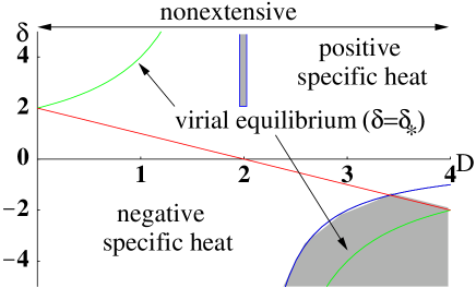
Figure 2: Stability chart for the gravity case ($\alpha=D-2$). The dark region corresponds to the stable region (79) in the parameter space ($\delta$, $D$). The property of the specific heat and the extensivity also are shown.

V Discussion

We studied the self-similar stationary solution in collisionless Boltzmann equation with the attractive $1/r^{\alpha}$ potential. Assuming the spherical symmetric and isotropic orbit in D-dimensional space, we investigate the linear stability of the solution. In the above model, we can control the extensivity of the system and the signature of the specific heat by changing the spatial dimension $D$ and the exponent of inverse power of the potential $\alpha$.

The self-similar stationary solution can be expressed in the form of the power law of the energy. The exponent of the power is determined by the power of the potential $\alpha$, spatial dimension $D$, and the scaling parameter $\delta$. Here we interpret $\delta$ as a parameter which denotes the virial ratio of the initial state.

By use of the energy functional approach, we investigated the stability of the self-similar stationary solution in terms of a symplectic linear perturbation. As for the spherical symmetric and isotropic orbit of the gravity in D-dimensional space ($\alpha=D-2$), we found that the system is stable if the mass distribution function decreases monotonically and the spatial dimension is less than 4. As for the power-law potential in one-dimensional space ($D=1$), we found that the system is stable if the mass distribution function decreases monotonically and the inverse power index of the potential is less than 2. The self-gravitating ring modelsota is similar to the case of $\alpha=1$ in one-dimensional space. From the form of the velocity distribution obtained by a numerical simulation, $\delta\sim-3$. This case belongs to the stable self-similar stationary solution.

The stable self-similar stationary solution we obtained includes the virial equilibrium state in the case of $\delta=\delta_{*}$ As for the extensivity of the system, the nonextensive system has far more stable scaling solutions than the extensive system in the parameter space ($\delta$, $\alpha$, $D$).

In the time evolution of the collisionless system, assuming the spherical symmetry and isothermal case, Larson-Penston solution which shows self-similar collapse is the attractorhanawa97 . By such a self-similar time evolution of system, we expect that the class of the stable self-similar stationary solution obtained in this paper plays an important role as a quasi-equilibrium state with a long range interaction such as gravity. In the realistic situation, since the anisotropic velocity space is important, we would like to extend this analysis to the anisotropic case in our future work.

Appendix A Transformation to self-similar coordinate

Using the original coordinate $(r,v)$, the self-similar coordinate $(R,X)$ is defined by

$$R := \delta^{-1}\ln(r|\delta|),$$ (80)

$$X := ve^{-\nu R}.$$ (81)

The derivative with respect to the original coordinate can be expressed by the self-similar coordinate in the form:

$$\partial_{r} = \left(\frac{\partial R}{\partial r}\right)\Big{|}_{X}\partial_{R}+\left(\frac{\partial X}{\partial r}\right)\Big{|}_{R}\partial_{X},$$ (82)

$$= \mbox{sgn}(\delta)e^{-\delta R}\left(\partial_{R}-\nu X\partial_{X}\right)$$

$$\partial_{v} = \left(\frac{\partial X}{\partial v}\right)\Big{|}_{R}\partial_{X}=e^{-\nu R}\partial_{X}.$$ (83)

Appendix B Stability condition for gravity case in $D=1$ and $2$ ($\alpha=D-2$)

For the case that the potential $\overline{\Phi}$ is positive, Eq.(22) is modified as

$$2\nu^{2}\left[2+(D-2)\frac{\delta}{\nu}\right]\overline{\Phi} = S_{D}^{2}G\int_{0}^{\infty}\!\!\!\!\!\!\!\!X^{D-1}\overline{f}dX.$$ (84)

B.1 $D=1$ case

Since the potential $\overline{\Phi}$ is positive, from Eq.(84),

$$\delta < 2.$$ (85)

By integrating Eq.(84), we have a self-similar solution (23) and

$$C=\frac{\left|2-\delta\right|\Gamma(\delta-1/2)|2\overline{\Phi}|^{\delta}}{\sqrt{\pi}G\Gamma(\delta-1)},$$ (86)

if the following condition is satisfied:

$$\delta > 1.$$ (87)

From Eqs. (85), (87), (63) and (76), the stability condition for linear perturbation yields

$$1<\delta<2.$$ (88)

The ratio of the average of the kinetic energy to the potential energy is the same as Eq.(31) in $D=1$. However, if $\delta\leq 2$, the integral of the kinetic energy over the velocity space diverges. For this reason, there do not exist a stable self-similar stationary solution in $D=1$.

B.2 $D=2$ case

If the potential $\overline{\Phi}$ is negative, the condition that the bounded self-similar solution exists is the same as Eqs.(25) and (26). Since this case does not satisfy the condition (26), the only case is that $\overline{\Phi}>0$.

In this case, from Eq.(84), the condition that a bounded self-similar solution exists yields

$$\delta > \frac{1}{2},$$ (89)

and the integral constant of (23) is

$$C=\frac{2\Gamma(\delta)|2\overline{\Phi}|^{\delta}}{\pi^{5/2}G\Gamma(\delta-1/2)}.$$ (90)

From Eqs. (63), (76), and (89), the stability condition against linear perturbation yields

$$\delta > \frac{1}{2}.$$ (91)

The ratio of the average of the kinetic energy to the potential energy is the same as Eq.(31) in $D=2$. However, similar to the $D=1$ case, if $\delta\leq 2$, the integral of the kinetic energy over the velocity space diverges. Finally, if $\delta>2$, the self-similar stationary solution in $D=2$ is stable. In this case, the specific heat is always positive.

References

• (1) R.B. Larson, Mon. R. astron. Soc.194 (1981), 809.
• (2) E. Falgarone, T.G. Phillips, and C.K. Walker, ApJ.378 (1991), 186.
• (3) D. Merritt and T. Fridman, ApJ.460 (1996), 136.
• (4) F.S. Labini, M. Montuori, and L. Pietronero, Phys. Rep.61 (1998), 293.
• (5) J.F. Navarro, C.S. Frenk, and S.D.M. White, ApJ.490 (1997), 493.
• (6) T. Fukushige and J. Makino, ApJ.557 (2001), 533.
• (7) Y. Sota, O. Iguchi, M. Morikawa, T. Tatekawa, and K. Maeda, Phys. Rev. E 64 (2001), 056133.
• (8) I. Ispolatov and E.D.G. Cohen, Phys. Rev. Lett. 87 (2001), 210601.
• (9) A. Campa, A. Giansanti, D. Moroni, and C. Tsallis, Phys. Lett. A 286 (2001), 251.
• (10) A. Campa, A. Giansanti, and D. Moroni, Physica  A 305 (2002), 137.
• (11) H.E. Kandrup, ApJ.351 (1990), 104.
• (12) H.E. Kandrup, ApJ.370 (1991), 312.
• (13) J. Perez and J.J. Aly, Mon. Not. R. Astron. Soc.280 (1996), 689.
• (14) J. Perez and M. Lachieze-Rey, ApJ.465 (1996), 54.
• (15) P. Jund, S.G. Kim, and C. Tsallis, Phys. Rev. B 52 (1995), 50.
• (16) R.H. Henriksen and L.M.Widrow, Mon. Not. R. Astron. Soc.276 (1995), 679.
• (17) B. Carter and R.H. Henriksen, J. Math. Phys.32 (1991), 2580.
• (18) J. Binney and S. Tremaine, Galactic Dynamics.
( Princeton Univ. Press, Princeton ) (1993).
• (19) V.A. Antonov, Sov. Astron.4 (1961), 859.
• (20) V.A. Antonov, Vestnik Leningrad Univ.7 (1962), 135.
• (21) D. Lynden-bell and N. Sannit, Mon. Not. R. Astron. Soc.143 (1969), 167.
• (22) J.R. Ipser, ApJ.232 (1974), 863.
• (23) J.F. Sygnet, G. Des Forets, M. Lachieze-Rey, and R. Pellat, ApJ.276 (1984), 737.
• (24) P. Bartholomew, Mon. Not. R. Astron. Soc.151 (1971), 333.
• (25) D.D. Holm, J.E. Marden, T. Ratiu, and A. Weinstein, Phys. Rep.123(1985), 1.
• (26) T. Hanawa and K. Nakamura, ApJ.484 (1997), 238.