Distant Cluster Hunting II: A Comparison of X-ray and Optical Cluster Detection Techniques and Catalogs from the ROX Survey

Abstract

We present and analyze the optical and X-ray catalogs of moderate-redshift cluster candidates from the ROSAT Optical X-ray Survey, or ROXS. The survey covers the sky area contained in the fields of view of 23 deep archival ROSAT PSPC pointings, 4.8 square degrees. The cross-correlated cluster catalogs were constructed by comparing two independent catalogs extracted from the optical and X-ray bandpasses, using a matched-filter technique for the optical data and a wavelet technique for the X-ray data. We cross-identified cluster candidates in each catalog. As reported in Paper I, the matched-filter technique found optical counterparts for at least 60% (26 out of 43) of the X-ray cluster candidates; the estimated redshifts from the matched filter algorithm agree with at least 7 of 11 spectroscopic confirmations ($\Delta z\lesssim 0.10$). The matched filter technique, with an imaging sensitivity of $m_{I}\sim 23$, identified approximately 3 times the number of candidates (155 candidates, 142 with a detection confidence $>3\sigma$) found in the X-ray survey of nearly the same area. There are 57 X-ray candidates, 43 of which are unobscured by scattered light or bright stars in the optical images. Twenty-six of these have fairly secure optical counterparts. We find that the matched filter algorithm, when applied to images with galaxy flux sensitivies of $m_{I}\sim 23$, is fairly well-matched to discovering $z\leq 1$ clusters detected by wavelets in ROSAT PSPC exposures of 8,000-60,000 seconds. The difference in the spurious fractions between the optical and X-ray (30% and 10% respectively) can not account for the difference in source number. In Paper I, we compared the optical and X-ray cluster luminosity functions and we found that the luminosity functions are consistent if the relationship between X-ray and optical luminosities is steep ($L_{x}\propto L_{opt}^{3-4}$). Here, in Paper II, we present the cluster catalogs and a numerical simulation of the ROXS. We also present color-magnitude plots for several of the cluster candidates, and examine the prominence of the red sequence in each. We find that the X-ray clusters in our survey do not all have a prominent red sequence. We conclude that while the red sequence may be a distinct feature in the color magnitude plots for virialized massive clusters, it may be less distinct in lower-mass clusters of galaxies at even moderate redshifts. Multiple, complementary methods of selecting and defining clusters may be essential, particularly at high redshift where all methods start to run into completeness limits, incomplete understanding of physical evolution, and projection effects.

1 Introduction: Why Conduct an Optical - X-ray Survey for Clusters of Galaxies?

Clusters of galaxies are the most massive gravitationally-bound systems in the universe. Because they sample the high mass end of the mass function of collapsed systems, they can be used to determine cosmological parameters such as $\Omega_{m}$ (e.g. Donahue & Voit 1999). The largest clusters ($\sim 10^{15}~{}M_{\odot}$), are the products of the collapse of matter from a very large volume of space ($r\sim 16h^{-1}(\Omega/0.2)^{-1/3}~{}\rm{Mpc}$). Therefore they are thought to be “fair samples” of the universe – that the mass to light ratio or the baryonic mass fraction defined within the domain of a cluster of galaxies is representative of that ratio in the universe as a whole. They are purported to be “closed boxes” to star formation and evolutionary processes that occur within their domain. In this paper we present and analyze the catalogs from our joint optical-X-ray search for clusters of galaxies. We conducted this survey in order to provide a sample of clusters to test such assumptions about clusters of galaxies and to investigate the impact of sample selection on studies of cluster evolution and the evolution of their member galaxies.

Understanding cosmological or galaxy evolution studies of clusters critically requires an understanding of the biases in any sample of clusters. For example, the evolution of the number density of systems with cluster-sized masses as a function of mass and redshift is a fundamental prediction of cosmological structure formation models. To know the number density of clusters, we must know the biases inherent in how we find them, preferably as a function of cluster mass. Furthermore, testing the “fair sample” hypothesis requires reliable and unbiased selection of the most massive clusters.

Ever since Abell (1958) and Zwicky (Herzog, Wild & Zwicky 1957; Zwicky 1961) began publishing catalogues of optically selected clusters of galaxies, the definition of a cluster and the definition of biases inherent in the cluster detection process have been lively topics of debate. In 1978, the launch of the first X-ray imaging telescope, the Einstein observatory, began a new era of cluster discovery, as clusters proved to be luminous ($>10^{42-45}{\rm erg\,s^{-1}}$), extended ($r\sim 1-5$ Mpc) X-ray sources, readily identified in the X-ray sky. The intracluster gas, in nearly hydrostatic equilibrium with the gravitational potential of the cluster, radiates optically thin thermal bremstrahlung and line radiation. X-ray selection of clusters is more robust against contamination along the line of sight than traditional optical methods since the richest clusters are relatively rare and since X-ray emissivity, which is proportional to the gas density squared, is far more sensitive to physical overdensities than is the projected number density of galaxies on the sky.

One cluster sample differs from another depending on how the clusters were detected. Optical selection of clusters using traditional methods looking for overdensities of galaxy counts (e.g. Abell 1958) was rife with contamination problems. However, modern methods such as the “matched filter” algorithm (Postman et al. 1996, P96 hereafter) provide automated, uniform detection of galaxy overdensities in deep optical images. The matched filter technique searches for local density enhancements in which galaxies follow a magnitude distribution characteristic of that expected for a cluster of galaxies. The results include statistically quantifiable estimates of cluster richness, redshift, and significance. The first X-ray selection methods using sliding boxes were optimal for point sources. Thus, the detection method used to construct the Extended Medium Sensitivity Survey (EMSS; Gioia et al. 1990b) was biased somewhat towards selecting clusters with high central surface brightnesses. Now there are several algorithms optimized for detecting extended sources, including wavelets (Rosati et al. 1995) and Voronoi-Tesselation Percolation methods (Scharf et al. 1997).

A decade ago, optical and X-ray surveys apparently disagreed about how much clusters have evolved since $z\sim 0.5-1.0$. Optical surveys indicated very little evolution since $z\sim 0.5-1$ (Gunn, Hoessel & Oke 1986), but the accurate measurements of survey volumes and cluster properties required for quantitative assessment of this evolution were difficult to quantify in these first high-redshift cluster surveys and the volumes were small so uncertainties were large. X-ray studies suggested modest evolution (Gioia et al. 1990a). The most recently compiled X-ray samples of clusters over a range of redshifts out to $z\sim 0.8-1.2$ agree that the X-ray luminosity function for moderate luminosity clusters has not evolved significantly since $z\sim 0.8$ (Borgani et al. 1999; Nichol et al. 1999; Rosati et al. 1998, 2000; Jones et al. 1998), while the most luminous systems, contained in the EMSS, might have evolved somewhat (Henry et al. 1992; Nichol et al. 1997, Vikhlinin et al 1998, 2000; Gioia et al. 2001) or very little (Lewis et al. 2002). More recent optical surveys for distant clusters continue to find very little evidence for cluster number density evolution at moderate redshifts (Couch et al. 1991; P96). The explanation of what may seem like a persisting discrepancy is that if any evolution exists in the X-ray cluster population, it is only occuring in the highest luminosity systems which are also the most rare systems. The optical surveys of Couch et al. (1991) and P96 were too small and shallow to detect the putative evolution of the rarest systems.

While the most recent optical and X-ray results are now at least in statistical agreement on the question of evolution since $z<0.8$, the question remains whether both techniques are selecting the same clusters. The fundamental quantity, from the viewpoint of comparison to cosmological simulations, is the cluster’s mass. We do not know a priori whether optical luminosity or X-ray luminosity should be better correlated with a cluster’s mass. The fundamental question, from the viewpoint of “fair sample” techniques of measuring universal ratios, is whether clusters are truly a “fair sample”. For example, M/L ratios depend on the bandpass of the light and the star formation history of the constituent galaxies. If the gas fractions or the M/L ratios vary significantly from cluster to cluster they are obviously not representative of the universe as a whole.

X-ray selection is generally thought to be superior to optical selection. Observationally, the hot gas is a larger fraction of the cluster mass than the stellar mass, and the X-ray luminosity of a cluster is far easier to measure than its optical luminosity. For X-ray selected clusters, studies of gas fractions and cluster M/L ratios show that these quantitites are statistically constant (Evrard 1997; Arnaud & Evrard 1999; Carlberg et al. 1996). However, if X-ray selection biases the selection of the clusters, high-mass clusters of galaxies with low hot gas fractions (if they exist) would be omitted from such studies. Massive clusters, under the “fair sample” hypothesis, should have nearly identical baryon fractions, however they are discovered.

With the ROSAT Optical X-ray Survey (ROXS) for clusters of galaxies, we have endeavored to address such issues by obtaining optical images of complete 30’ by 30’ fields centered on positions of deep ROSAT PSPC pointings. In contrast to previous ROSAT PSPC serendipitous surveys such as those conducted by Rosati et al. (1995, 1998), Jones et al. (1998), Romer et al. (2000), and Vikhlinin et al. (1998), the ROXS includes optical imaging for the entire field of view of each X-ray pointing. The X-ray selection and optical selection of cluster candidates was then done independently of each other. We observed 23 ROSAT pointings for a total of nearly 5 square degrees in I band. For five of these fields we also obtained V-band imaging. In this paper (Paper II) we present the catalogs, survey windowing functions, data reduction and observation details, an analysis of detection likelihoods, as well as an expanded discussion and further analysis, including numerical simulations of the survey. In §2, we describe the X-ray field selection criteria and the optical observations. In §3, we present the optical cluster candidates catalog, cross-identification of clusters in the V and I bands. In §4, we present the X-ray cluster candidate catalogs and the X-ray/optical cross-identification procedure. In §5 we describe properties of the cluster candidates, including the distribution of observed properties of objects in the sample, the estimated richness vs. $L_{x}$, the $V-I$ vs $I$ color magnitude diagrams for the clusters identified in both the $V$ and $I$ bands. We discuss and summarize our results in §6 and §7 respectively.

For all derived quantities, we have used $H_{0}=75h_{75}$ km s^-1 Mpc^-1, and $q_{0}=0.5$.

2 Observing Strategy, Observations and Data Reduction

2.1 Field Selection and Observations

The sample of 23 target fields were chosen from a sample of archival X-ray observations. All ROSAT PSPC pointings with exposure times of more than 8,000 seconds and Galactic latitude of $|b_{II}|>20$ degrees and declination $\delta>-20$ degrees were considered for optical imaging from Kitt Peak. We avoided fields with bright stars $(m_{V}<9)$. Even so, bright stars outside the field occasionally scattered light into the field of view and stars with $m_{I}<16$ had diffraction spikes. Pixels affected by bright stars and scattered light were masked in our subsequent analysis, and thus the total survey area is 4.8 square degrees, less than the nominal 5.75 square degrees that would have been covered if optical detection success were unaffected by stars. Table 1 summarizes the fields observed as well as the associated data.

We obtained the optical data during two observing runs at the Kitt Peak National Observatory 4-meter telescope during March 1996, and May 1997. We were awarded 4 observing runs for this project, but one (November 1995) was cancelled because the dome mechanism was broken and another had extremely poor weather (November 1996). Therefore, the entire survey was conducted in the northern spring sky. The KPNO 4-meter prime focus CCD camera T2KB has a 16’ field of view (0.47” pixel^-1). We mosaiced $2\times 2$ of these fields to created full 30’ by 30’ fields, each centered on a deep ROSAT pointing, overlapping each quadrant by $\sim 1^{\prime}$.

A total of 900 seconds of exposure were obtained through the I-band filter for each ROSAT field quadrant. Our 5$\sigma$ detection limit of $I=23$ (Vega magnitude) was sufficient to detect cluster galaxies 2 magnitudes fainter than the typical unevolved first-ranked elliptical at $z=1$ (Postman et al. 1998a). For five of the ROX fields, we also obtained V-band data, for a total exposure of 600 seconds for each quadrant. The data were obtained under near photometric conditions and low air masses ($<1.2$, typically). When the sky was photometric, we obtained short exposures of the center of each field for calibration purposes, and thus all of our data were flux-calibrated (see §3.1.1). The filters used were the V and I filters from the Harris set.

2.2 Data Reduction

The CCD images were first reduced with standard IRAF tools for bias level subtraction, frame trimming, and flat-field division. A cosmic ray rejection algorithm based on median filtering techniques was used to remove cosmic rays from the images. In the first observing run, each pointing was divided into two 450 second exposures because the I-band sky was so bright that the dynamic range of the A-to-D converter was swamped. We used the two images to reject cosmic rays. For our second run, the A-to-D converter had been updated to unsigned integers, and the cosmic-ray rejection made possible with two images was determined to be of little advantage compared to the overhead time and additional data-reduction complexity. Data obtained during subsequent telescope visits thus consisted of single 900-second observations. The two 450 second exposures for each quadrant obtained in earlier runs were coadded. We achieved a detection limit of $23$ mags in I and $24$ mags in V (Vega magnitudes).

To prepare for the galaxy catalog construction, the following processing steps as discussed in P96 were employed. A sky model for each (coadded) frame was created from the data to remove the remaining CCD signatures. We fit the median sky level as a function of row, and subtracted the appropriate sky components from each image row. These steps produced frames with extremely flat sky levels.

3 Catalogs

Here we describe the procedures and assumptions we used to create the galaxy catalog, the matched filter cluster catalog, the X-ray catalog, and the cross-identifications of probable detections of the same physical cluster system.

3.1 Optical Catalog

3.1.1 Galaxy Catalog Construction

We followed the procedures discussed in P96 to construct the galaxy catalog. A modified version of the Faint Object Classification and Analysis System (Jarvis & Tyson 1981, Valdes 1982) was used to detect, measure, and classify objects in the calibrated CCD images. The detection algorithm estimated a point spread function (PSF) for each frame, to compensate for seeing variations from exposure to exposure. To separate stars from galaxies, FOCAS classification parameters were chosen to cover PSF variations but to be robust to star-galaxy distinctions. Perfection in distinguishing galaxies from stars is not critical to our experiment since galaxies dominate the detected object counts in the magnitude range of interest (P96).

Astrometric calibration was performed by selecting unsaturated bright stars. The J2000 celestial positions of the stars were measured from the Digitized Sky Survey (the “Quick V” survey, epoch 1983) based on Palomar Observatory Schmidt plates (Lasker et al. 1990). An astrometric solution was computed based on a 6-term per coordinate polynomial for each field. Typical solution uncertainty is $<0.5"$. The absolute photometry for Johnson V and Cousins I fluxes was obtained using Harris V and I-band observations of Landolt Standards fields PG1047+003, 1159-035, SA107, and PG1657+078 (Landolt 1992). For our figures and tables we use Johnson V and Cousins I. Those magnitudes are related to AB magnitudes using the following relations. $V(Johnson)=V(AB)-0.02$ and $I(Cousins)=I(AB)-0.45$.

3.1.2 Cluster Catalog Construction

The procedures in P96 were followed in constructing the cluster catalog. The algorithm based on the matched filter method, tuned to redshifts in the range $0.2<z<1.2$, was used to generate cluster catalogs in $\Delta z=0.1$ intervals. $H_{0}=75h_{75}$ km s^-1 Mpc^-1 and $q_{0}=0.5$ were assumed for all quantities. Clusters were identified by searching for the local maxima within a moving box which was $1.667h_{75}^{-1}$ Mpc across. A candidate cluster was registered when the central pixel in the box was the local maximum and it lay above a prescribed threshold. We used the following cluster detection parameters and cluster assumptions to generate the cluster catalog. The slope of the radial filter profile was 1.40. A cluster core radius of $133.3h_{75}^{-1}$ kpc was assumed, and the smoothed map was sampled every 0.50 core radii. The cut-off radius for cluster detection was set to $1333h_{75}^{-1}$ kpc, with a detection box half-width of $1666.7h_{75}^{-1}$ kpc. The profile kernel halfwidth was 20 map pixels, defined by the 0.50 core radius for each map, the catalog scale was 1 arcsecond/unit, and the CCD scale was 0.45 arcsecond/pixel. For the luminosity function filter we assumed a Schechter function (Schechter 1976) with $M^{*}=-21.0+5\log h_{75}$ in the V band and $M^{*}=-21.90+5\log h_{75}$ in the I band with a slope of -1.10 for both bands. Each cluster candidate is assigned a central position, effective radius (corresponding to the area of detection equal to $\pi r_{eff}^{2}$), an estimated redshift based on the best-fit luminosity function, an average galaxy magnitude ($I_{mag}$ or $V_{mag}$ depending on the bandpass), and a detection confidence in units of sigma ($\sigma$). The algorithm also estimates an effective optical luminosity $\Lambda_{cl}$, which corresponds to the equivalent number of $L^{*}$ galaxies in the cluster such that the optical cluster luminosity $L_{cl}/L_{\odot}=\Lambda_{cl}L^{*}/L_{\odot}=\Lambda_{cl}10^{-0.4(M_{\odot}-M^{*})}$ where $M_{\odot}$ is the absolute magnitude of the Sun in the appropriate band (P96). The quantity $\Lambda_{cl}$ is relatively insensitive to $H_{0}$; variations $\sim 5\%$ were measured if $h_{75}=1.33$ rather than 1.0. For reference, a richness class 1 cluster at $z\leq 0.7$ had $\Lambda_{cl}=30-65$ in the I-band (P96).

These parameters generated cluster catalogs that are directly comparable to cluster candidates in the Postman et al. (1998b) 16 square degree I-band survey (called “Deeprange”). The similarity in optical methods and instrumentation for the ROXS and the Deeprange surveys allowed us to compare the spurious rates of cluster identification and the reliability of the estimated redshifts with respect to spectroscopic redshifts for the ROXS from the larger Deeprange survey, in addition to the P96 survey.

Table 2 lists the cluster candidates for 23 fields observed. We have extracted the optical selection function as a function of redshift in Figure 1. These probabilities were computed following P96, assuming a K-correction appropriate to a galaxy population dominated by ellipticals.

3.2 V and I band Cross-Identifications

Here we describe the comparison of the cluster candidate catalogs resulting from the matched filter algorithm for the I-band data and the V-band data that we obtained for five of the ROXS fields. We find that 60-65% of the clusters identified in the I band are also detected in the V-band with similar estimated redshifts if we exclude all candidates with high redshift estimates ($z>1$).

For five fields (Table 1), we obtained V-band images, with a source detection limit $V_{AB}\sim 24$ magnitudes within an exposure time of $600$ seconds. We used the matched filter algorithm, adjusted for the V-band to provide appropriate estimated redshift estimates and $\Lambda_{cl}$, to provide an independent sample of optical candidates. In the five fields, we found 46 V-band candidates with a detection confidence of $>3\sigma$ and 33 I-band candidates with a $>3\sigma$ confidence.

When we cross-identify the candidates from the I-band and the V-band, we find that of the 33 I-band candidates, there are positional matches for 15 candidates with one or more V-band candidates (Table 3). All but one of these 15 candidates also match in estimated redshift ($\Delta z\leq 0.1$). Regions in the V-band images containing 6 I-band candidates were seriously affected by scattered light or bright stars – a more serious observational effect at V than at I. Therefore, a maximum of 27 of the I-band clusters could have been detected in V band. Of those 27, 4 were high redshift candidates ($z\geq 1$), leading to a V-band detection rate of $z<1$ I-band candidates of 15/23 or 65% (Table 5). The failure to detect high-redshift I-band candidates in the V-band is not unexpected since the 4000-Angstrom break spectral feature would make the elliptical galaxies in such clusters, even if the clusters are real, very difficult to see in the V-band. Additionally, the matched filter algorithm reliability degrades rapidly for our I-band data at redshifts greater than $\sim 1$ because that is where the faint end of the luminosity function is severely truncated by the survey magnitude limit. In this regime, corrections for the missing optical light are only mildly reliable and the result is a significantly higher error in the derived $\Lambda_{cl}$ value.

Correspondingly, of the 46 V-band candidates, 18 had one or more counterparts in the I-band (20 with a detection significance $>2.9\sigma$), and only 2 candidates were undetectable because of stray light in the I-band image, for a detection fraction of 18/44 or 41%. This detection fraction has been diluted by many high redshift V-band candidates with no I-band counterparts (15 with $z>1$). We suspect that all of the 17 $z>1$ V-band candidates may be spurious. Of the two high redshift V-band candidates with plausible I-band counterparts, one has a loose association with a $z=1$ I-band candidate (120436.7+280520, OC4 in the 1202+281 field) and the other (154923+212325, OC3 in the 3C324 field) has an estimated redshift of 0.7 from the I-band data, compared to the V-band estimate of 1.2.

We expect that the reliability of the matched filter method may become poor for the highest estimated redshifts, especially in the V-band for the following reasons. At the highest redshifts, the luminosity function filtering algorithm in the matched filter cluster detection method is only sensitive to the brightest galaxies in a cluster, especially for the V-band where K-correction effects are strongest. Moreover, the contrast of the most distant clusters against the foreground/background galaxy population becomes very weak, especially at bluer wavelengths due to the combination of K-correction effects and the steeper number counts of faint field galaxies (themselves potentially clustered) at bluer wavelengths.

We can therefore provide plausible explanations for many if not all of the failures to cross-correlate between I-band identifications and V-band identifications (Table 4) by a cluster candidate (either in I or V) with a high estimated redshift which may be a warning flag for unreliable or weak detections, or by obscuration or confusion with scattered light or spikes from bright stars.

Our resulting efficiency in cross-identifying clusters in either V-band or I-band is $\sim 60-65\%$, for candidates with estimated redshifts of $z<1$ and if we correct for the candidates which are detected through one filter but undetectable in the other because of scattered light. We present a summary of our numbers in Table 5.

We cannot explain the failure to detect 8 I-band cluster candidates of moderate redshift in V. Four of these candidates have possible V-band counterparts with redshifts from the V-band data similar to those derived from the I-band data, but with low detection significance or with centroids separated by $>3-4^{\prime}$. These possible counterparts are listed in Table 3. We also cannot explain the lack of an I-band counterpart for 11 V-band cluster candidates of moderate redshift (as in I band, 3 of these candidates have low significance counterparts or widely separated I-band counterparts with similar redshift estimates). We note that while the detection significance of these unmatched cluster candidates is similar to the rest of the sample (not much dynamic range), the estimated richnesses tend to be rather low $\Lambda_{cl}~{}20-50$, mostly $\leq 30$. We could be seeing incompleteness effects rather than spurious effects at lower $\Lambda_{cl}$, but it is possible that some of these unconfirmed cluster candidates are false.

If we count only the most secure cross-identifications, the I- and V-band cross identification statistics imply a spurious fraction of $<35\%$ for matched filter candidates with estimated cluster redshifts of less than one – consistent with the estimates of the spurious fraction of 25-30% from the Deeprange survey (Postman et al 1998b), with simulations done in P96 and in Postman et al (in preparation), and with spectroscopic observations (for $z<0.6$) in Postman et al. (in preparation). The spurious fraction for candidates with estimated redshifts larger than one is completely unknown since no candidate with $z\geq 1$ in one bandpass has a secure counterpart in the other bandpass.

Comparison of matched filter results from the I and V band do not address important sources of spurious cluster candidates, such as unbound aggregates of galaxies seen in a “pole-on” filament. Both the I- and V-band data would be contaminated by such structures. For this reason, comparision of the matched filter method with X-ray observations and other cluster detection methods, such as Sunyaev-Zel’dovich or weak-lensing observations and spectroscopy of member galaxies is critical. With ROXS, we make the direct comparison with the X-ray observations; in this paper, we provide the catalogs of optical and X-ray candidates for follow-up with other cluster hunting techniques.

4 X-ray Catalog

Here we describe the creation of the catalog of X-ray cluster candidates and the cross identification of X-ray candidates with optical candidates detected by the matched filter algorithm in the I-band images.

4.1 X-ray Source Detection and Upper Limits for Optical Sources

A wavelet-based technique, described by Rosati et al. (1995), was used to create an catalog of X-ray clusters of galaxy candidates for each field observed at Kitt Peak. Several of these fields overlapped with the orginal ROSAT Deep Cluster Survey (RDCS; Rosati et al. 1995, 1998) sample, and thus the X-ray cluster candidates in some of the fields already have been confirmed and have spectroscopic redshifts. The flux limits for ROXS are approximately the same as those of the RDCS ($F_{x}>10^{-14}~{}{\rm erg\,s^{-1}\,cm^{-2}}$), but of course vary with exposure time in both surveys. Table 6 lists the 57 X-ray candidate clusters and their associated X-ray parameters for each ROSAT field, and the spectroscopic redshift, when available. The X-ray parameters (Table6) measured are a centroid position (RA and Dec J2000), the net number of X-ray photons in the source (Counts), the off-axis angle of the source in arcminutes (Theta), the FWHM of the source in arcseconds (FWHM), the confidence level of the extended nature of the source in $\sigma$ (Sig-ext), and the X-ray flux and error in the 0.5-2.0 keV bandpass ($F_{x}$ and $eF_{x}$). The comment field includes the spectroscopic redshift, if available. A notation of ”d” indicates the source may be a double source. Occasionally, a source has a large flux error, reflecting not the confidence in the detection, but the uncertainty in measuring the flux from an extended, complex object.

A by-product of our analysis was a catalog of all the X-ray point sources in the field down to the flux limit of each ROSAT observation. These sources matched very nearly one-to-one to sources available in the WGACAT (White, Giommi, Angelini 1995), so we do not list them here. We will provide this list on request. In Table 2, we identify the optical candidates without an associated extended X-ray source but with an X-ray point source within 30-60”.

For every optical cluster candidate, we estimated the X-ray detection threshold defined by an upper limit to the observed $0.5-2$ keV flux as the flux corresponding to a $4\sigma$ fluctuation above the limiting surface brightness, within a $r=1^{\prime}$ aperture, as a function of position in the ROSAT field of view. The variation of X-ray source detection efficiency, arising from the degradation of the Point Source Function (PSF), as a function of off-axis angle can be seen in Figure 2 where we plot the mean number of X-ray sources per unit area in radial bins. There is almost a factor of ten reduction in the source counts at the largest off-axis angles. This reduction corresponds to as much as a factor of $4-5$ change in the flux limit, which is taken into account in our upper-limit estimates in Table 2. Using the known, deep, cumulative source number counts in the $0.5-2$ keV band (e.g. Hasinger et al. 1998) we can map the trend seen in Figure 2 into flux-limit vs off-axis angle. A simple, approximate, linear fit to this yields a relationship of (in units of $10^{-14}$ erg s^-1 cm^-2 ($0.5-2$ keV)): $f_{lim}\simeq A+0.078\theta$, where A is the flux limit at $\theta=0^{\prime}$ and $\theta$ is the off-axis angle in units of arcminutes. Since our X-ray detection algorithm provides us with an estimate of the background surface brightness we can normalize the above relationship with the flux of a $4\sigma$, on-axis source in a given aperture, and for a given field. The detection thresholds $F_{lim}$ in units of $10^{-14}$ erg s^-1 cm^-2 ($0.5-2.0$ keV) are reported in Table 2.

We convert the detection thresholds for the ROSAT fields into X-ray detection probabilities, as plotted in Figure 3, as a function of X-ray luminosity ($L_{x}$) and redshift, by assuming a canonical $L_{x}$-core radius relationship for the cluster surface brightness profiles (e.g. Jones et al. 1998). The cluster surface brightness profiles are assumed to be standard $\beta$-profiles with $\beta=2/3$. The detection probability is computed as the net probability to detect a cluster with a given redshift and $L_{x}$ in the entire ROXS coverage, based on exposure time, background surface brightness, and radial detection efficiency due to PSF variations discussed in the previous paragraph (Scharf et al. 1997; Rosati et al. 1995).

4.2 X-ray-Optical Cross-Identification

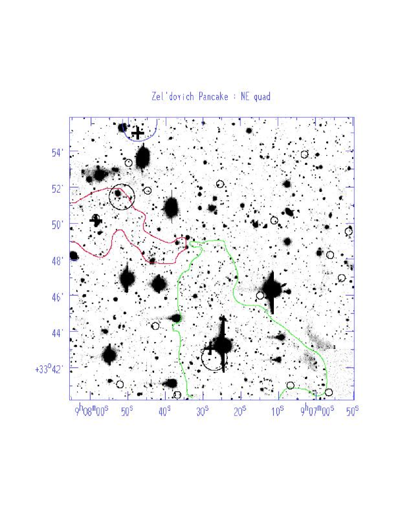
Figure 4: The rich northeast quadrant of the Zel’dovich Pancake field. X-ray point source detections are plotted as small circles. The large circles are extended X-ray sources. The optical cluster candidates are identified with crosses and single contours. In this quadrant there are 3 optical cluster candidates, two of which match an X-ray cluster candidate.

We cross-identified each X-ray candidate and I-band optical candidate by visually inspecting the overlap of the X-ray surface brightness contours and the optical contours of the detection thresholds for filtered optical maps at the nominal detected estimated redshift. Optical and X-ray contour shapes did not match in detail. Cluster candidates which overlapped significantly were identified as cross-identification candidates. We have noted the separation of the nominal optical and X-ray centroids in the tables. The centroid of the optical candidate could be shifted from the true position because of regions contaminated by bright stars, which must be masked from the data. The centroids of both X-ray and optical candidates are likely only to be good to $\pm 0.5^{\prime}$; cluster diameters at any redshift are usually $>2^{\prime}$. Typical centroid separations are $<2^{\prime}$. An example I-band image quadrant with the X-ray and optical sources labelled is shown in Figure 4.

As reported in Paper I, of the 57 X-ray candidates, 43 would have been visible on our optical frames (that is, not obscured by bright stars or scattered light). Of the 43, 29 were visually identified with potential cluster candidates with centroid separations of $\leq 3^{\prime}$ or with significant contour overlap, of which 26 are very secure (separations $\leq 2^{\prime}$ or visual confirmation of X-ray and optical correspondence of somewhat complex structure). The other three less secure identifications are more questionable affiliations of sprawling optical galaxy systems or filaments with a more compact X-ray cluster candidate. One such X-ray candidate, a confirmed cluster at $z=0.167$, MS1201+283 or Abell 1455, does not have a formal optical counterpart, but has up to 3 optical possible counterparts based on a visual inspection of the field. The optical field around this cluster was cut-up by bright stars, and the matched filter seems to have detected individual cluster candidates in the remnants.

The remaining 14 X-ray cluster candidates can be divided into 3 categories. Six candidates are bona fide, optically faint candidates, three of which have low-significance counterparts ($<3\sigma$) that are interesting because of their high estimated redshift, but they are not counted as true X-ray/optical coincidences. The other two categories contain sources that have a lower probability of a true cluster: double sources and sources with very uncertain X-ray fluxes ($F_{x}/\sigma_{F_{x}}<3$). There are two double sources without optical counterparts, and six sources with uncertain X-ray fluxes.

Only two of the optically-blank X-ray sources have yet been classified or confirmed at other wavelengths. One source (RXJ1256.9+4720) is tentatively associated with 3C280, the target of the original observation. Here we count this X-ray detection as an X-ray cluster candidate but not an optical cross-identification. It was the original target; this correspondence is the only example of the original target coinciding with a cluster candidate. The statistics are not skewed by the inclusion of this one very interesting cluster candidate. There was a $2\sigma$ detection at this position in the optical data. The estimated optical redshift ($z=1.0$) was so remarkably close to that of 3C280’s spectroscopic redshift ($z=0.997$) that we quote the matched-filter parameters of the optical candidate despite our extremely low confidence in its reality. We note that the 3C280 cluster only has one redshift in-hand, and a preliminary investigation of the Chandra image of this source shows X-ray structure associated with the radio source but no obvious cluster emission (M. Donahue, private communication.) The other candidate, RXJ1120.0+2115, was flagged as a double source; Rosati and his collaborators have found a cluster with $z=0.75$ (P. Rosati, private communication).

Since the spurious fraction typical of the X-ray surveys is $\sim 10\%$ (Rosati et al. 1998; Vikhlinin et al. 1998), approximately 6 of the 57 sources are expected to be false – X-ray sources which are not really extended or are constellations of point-like X-ray sources. Some of these candidates may be bona fide, albeit optically-faint clusters. Truly high redshift clusters are very faint in the I-band because of the 4000Å  break in elliptical galaxy spectra. Near IR imaging is probably the best tool to reveal the presence of any high redshift clusters.

Eleven X-ray candidates have confirmed spectroscopic redshifts from Rosati’s followup of clusters in the RDCS (Rosati et al., in preparation). We list the candidates in Table 7. All X-ray spectroscopic confirmations which were not obscured by bright stars had an optical counterpart with a detection confidence of $\geq 3\sigma$, except for the X-ray candidates associated with 3C280 at $z=1$ and with RXJ1120.0+2115, which now has a confirmed redshift of 0.75 (Rosati, private communication).

The redshift estimated by the matched filter algorithm has proven to be surprisingly good for the clusters of galaxies, at least for the X-ray selected clusters (Table 7). For 7 out of 11 extended X-ray sources with spectroscopic redshifts, the discrepancies between the photometric and the spectroscopic redshift are less than $\Delta z=0.1$, finer than our redshift grid. From Deeprange spectroscopic followup (Postman, private communication), the mean difference between spectroscopic and estimated redshifts for candidates with $0.3\leq z_{est}\leq 0.4$ is 0.04 with an rms scatter of 0.07, based on $\sim 25$ clusters. The scatter for all Deeprange candidates out to $z\sim 1$ is closer to 0.15 (Postman, private communication).

Of the five X-ray cluster candidates contained in the fields with both V-band and I-band data, all five were detected in both the V-band and I-band.

5 Cluster Candidate Properties

In this section we discuss the cluster properties such as X-ray luminosity, estimated for the cluster candidates in our samples. We find that while the cluster candidates in the ROXS sample have X-ray and optical properties consistent with the range of properties in other cluster samples, the clusters are somewhat less X-ray luminous, optically poorer, and have much less prominent sequences of red galaxies in color-magnitude diagrams than the typical rich and massive clusters of galaxies found in all-sky surveys. This sample thus may include cluster candidates that may be missed in pure X-ray, optical, or color searches for clusters. We make what may seem a pedantic distinction here: These clusters may be missed by a search not because the sample is incomplete, but because their properties fall outside the boundary of the sample selection function.

5.1 X-ray Luminosities

Here we show that the cluster luminosities are typical, with estimated bolometric $L_{x}\sim 10^{43}-10^{44}~{}{\rm erg\,s^{-1}}$, and that the upper limits are all $L_{x}\geq 10^{42}~{}{\rm erg\,s^{-1}}$. However, a couple of rich optical candidates are found with very low X-ray upper limits.

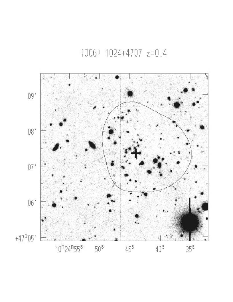
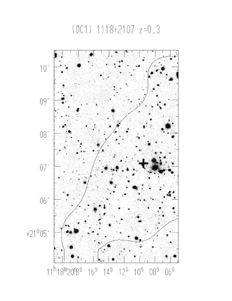
Figure 6: Two optical candidates with high detection significance from the matched filter algorithm ($>4\sigma$) but no associated X-ray flux, OC6 1024+4707 from the 1024+4707 field ($z=0.4$) and OC1 1118+2107 in the 1116+215 field ($z=0.3$).

The X-ray luminosity for each cluster candidate with an optical counterpart was computed assuming the matched-filter estimate for the cluster redshift, the X-ray flux from the wavelet detection algorithm, and a self-consistent bolometric correction commensurate with the X-ray temperature $T_{x}$ implied by the $L_{x}-T_{x}$ relation from Markevitch (1998). The $L_{x}-T_{x}$ relation is nearly constant with redshift (Donahue et al. 1999; Borgani et al. 2001). The optical cluster candidates which were not detected in the X-ray band all have X-ray upper limits from a $r=1^{\prime}$ aperture (see § 4.1), ranging from $2-10\times 10^{-14}{\rm erg\,s^{-1}\,cm^{-2}}$ (the bolometric corrections for the upper limits were computed assuming an X-ray temperature of $kT=4$ keV and the estimated redshifts). A mean $N_{H}=2.33\times 10^{20}$cm^-2 column density for high Galactic latitudes was assumed for all luminosities and upper limits. In Figure 5, we have plotted the distribution of estimated X-ray luminosities of cross-identified clusters and the upper limits of the optical candidates without X-ray counterparts. Note that none of the clusters are extremely luminous ($>6\times 10^{44}h_{75}^{-2}{\rm erg\,s^{-1}}$) and that none of the X-ray candidates has an X-ray luminosity upper limit significantly below a $2\times 10^{42}h_{75}^{-2}{\rm erg\,s^{-1}}$. Since this limit is approximately the luminosity of poor clusters, our X-ray data are not quite sensitive enough to rule out the presence of an X-ray group or low-luminosity X-ray cluster. However, a significant number of the optical candidates (54) have flux limits and estimated redshifts which imply X-ray cluster luminosities which are between $10^{42-43}h_{75}^{-2}{\rm erg\,s^{-1}}$, typical of luminosities of poor clusters of galaxies and even groups (Figure 5). Two such cluster candidates, with redshifts of 0.4 and 0.3 respectively, have $\Lambda_{cl}\geq 50$ (relatively rich) and upper limits on $L_{x}<10^{43}h_{75}^{-2}{\rm erg\,s^{-1}}$, clusters (OC1) 1118+2107 and (OC6) 1024+4707 (See Figure 6 for the I-band images of these candidates.) The optical detection significance for each of these two clusters was $\sim 5\sigma$. If these clusters turn out to be X-ray faint ($L_{x}$ significantly lower than that predicted by the $L_{x}-T_{x}$ or $L_{x}-\sigma_{v}$ relations for clusters), that would argue that X-ray surveys could miss some relatively massive systems. Such a hypothesis would be straightforward to test with XMM or Chandra X-ray imaging observations, alongside ground-based galaxy spectra to confirm the redshift and establish a velocity dispersion.

5.2 X-ray Luminosity - Optical Richness

Here we show that the X-ray luminosities and optical richness of the ROXS clusters are in the expected range and ratios typical of clusters of galaxies; however, as expected, the ROXS clusters are on average fainter in X-rays than those clusters selected from a very large area X-ray survey at much shallower X-ray flux depths.

In Paper I (Donahue et al. 2001) we evaluated the relationship between the X-ray luminosity $L_{x}$ and the estimate of optical luminosity $\Lambda_{cl}$ and while we found a marginally statistically significant correlation between these two properties, independent of estimated redshift, we also demonstrated that this relationship has significant scatter beyond that indicated by the estimated observational uncertainties.

To further investigate the relationship between the X-ray and optical properties of the ROXS we have compared the X-ray luminosities or upper limits and optical richnesses with those obtained from the Abell clusters composing the X-ray Brightest Abell-type Cluster Survey (XBACS) ROSAT survey of Ebeling et al (1996). The XBACS survey is composed of the Abell clusters detected in the northern portion of the Rosat All-Sky Survey, and therefore contains many high luminosity clusters of galaxies. Since such clusters are extremely rare, they are not expected in much smaller surveys such as ours. However, the X-ray luminosities spanned in ROXS are also spanned in the XBACS coverage, albeit for lower-redshift clusters.

We have combined the 283 XBACS X-ray luminosities with the Abell richness number counts $N_{R}$ from the Abell/ACO catalogue. For comparison to the ROXS, we have converted the matched filter richness parameter $\Lambda_{cl}$ (approximately equivalent to the number of $L^{*}$ galaxies in the system (P96)) to Abell richness counts $N_{R}$. However, as demonstrated in P96 the scatter between $\Lambda_{cl}$ and $N_{R}$, (where $N_{R}$ is defined as per Abell’s galaxy number counts within a $1.0$h^-1Mpc radius rather than Abell’s 1.5h^-1Mpc) is large, albeit with a positive correlation. For our purposes we use a relatively crude conversion from $\Lambda_{cl}$ to Abell counts; $N_{R}^{Abell}=(\Lambda_{cl}\pm 23)/0.72$, where the factor 0.72 converts galaxy counts from within a $1.0$h^-1Mpc radius to a 1.5h^-1Mpc radius (P96).

In Figure 7 panel (a) the X-ray luminosity (0.1-2.4 keV, converted to $H_{0}=75$ km s^-1 Mpc^-1, $q_{0}=0.5$) is plotted against $N_{R}^{Abell}$ for all XBACS clusters (open circles) and for all ROXS optical candidates with X-ray counterparts (filled circles). The uncertainties in the X-ray luminosities of ROXS clusters ranges from $\sim 7\%$ to $\sim 80\%$. In Figure 7 panel (b) the XBACS clusters are again plotted, but now with the upper limit on X-ray luminosities for all non-X-ray detected ROXS cluster candidates. The resulting relationship between Abell richness number counts and X-ray luminosity for ROXS plotted in Figure 7 has large scatter, a result consistent with our conclusions from Paper I (Donahue et al. 2001) and also with results from Borgani & Guzzo (2001), which we will discuss later.

It is also clear for both the X-ray detected and non-detected objects that the ROXS criteria tend to include more X-ray-poor systems than the Abell/ACO catalogue intersection with the XBACS. The XBACS half-sky survey has sufficient sky coverage and depth to find more luminous clusters, but it is not deep enough to detect proportionally as many X-ray faint clusters as are found in the ROXS survey. As we will also show in our red sequence analysis in § 5.5, the cluster candidates that we sample here are all likely to be somewhat lower in mass than their massive, X-ray luminous cousins found in surveys of larger sky area. The general form of the $L_{X}-N_{R}$ relationship of the ROXS cluster candidates is qualitatively similar to that found for the low-$L_{x}$ clusters in the XBACS,

5.3 Cluster-Point Source Correlation

One goal of our survey was to see whether a criterion of requiring cluster X-ray candidates to have significant extent in the ROSAT PSPC image filtered out clusters with X-ray emission too compact to be unambiguously resolved. Such a criterion could screen out high redshift sources or sources with prominent cooling flows. Since we were imaging complete fields we could investigate whether X-ray point sources, ignored by some cluster surveys, could actually be high-redshift or compact clusters.

Of the 142 optical candidate clusters with a detection confidence of $>3\sigma$, 27 have extended X-ray counterparts (one has two counterparts). Up to twenty-nine additional optical candidates have possibly interesting X-ray point sources either near the central core of galaxies (within 1’-2’) or near a possible cluster member. When an X-ray point source is near an optical candidate, we have indicated so in the Comments column of Table 2. For example, in the field of MKN 78, OC2 has a point source very close to it, RXJ0741.7+6525, an active galaxy with a redshift of 1.65 (RIXOS F234_001, with Mg II and CIII emission seen by Puchnarewicz et al. 1997). The estimated redshift of the cluster, however, is 0.4. In the field of 10214+4724, OC10 ($z=0.3$) is a compact optical candidate that is exactly coincident with the point source RXJ1025.4+4716; such exact alignments are worth investigating.

However, most of the point sources with positional coincidence with optical cluster candidates were not exact; coincidental alignments are likely, given the size of a typical cluster candidate. The number of coincidences between point sources and optical cluster candidates in our survey can be estimated by assuming that a typical optical cluster candidate has a radius of $\sim 100"$, and that the X-ray point source density at the 0.2-2.0 keV flux limit of $F_{x}\sim 10^{-14}{\rm erg\,s^{-1}\,cm^{-2}}$ is 100 sources deg^-2 (Rosati et al. 1998). With 142 optical candidates, the estimated number of chance coincidences is 34, comparable to the number that we identify. Therefore we do not detect a significant excess of X-ray point sources near optical cluster candidates.

In order to see whether the correspondence with point sources increased when we applied our judgement as to the reality of a cluster candidate, we visually inspected each optical candidate and assessed a subjective believability index to it, of “probable”, “blend”, or “unlikely”. This subjective assessment showed that many of the optical candidates are likely to be blends with other optical candidates at different redshifts. Lacking a purely objective means of sorting out blends, we have listed all blend candidates with notations in the Comments column (Table 2). Some 57 out of the 142 optical candidates without X-ray counterparts passed this subjectivity test; 17 of these may have associated point sources. The fraction of optical candidates without extended X-ray counterparts but with possible X-ray point source counterparts did not increase significantly with this subjective assessment. Therefore, we suspect that most of these associations are likely to be random projections of background AGN with the optical candidates.

We note the fraction of optical candidates which have X-ray counterparts or which are deemed believable in a subjective assessment is a strong function of detection confidence ($\sigma$) and estimated redshift. The percentage of X-ray clusters plus “probable” optical clusters is 70% of the total at $z=0.2$, dropping to 45% at $z=0.8$, and $0-20\%$ at $z=1.0-1.2$ (Figure 8a and  10). The same fraction as a function of $\Lambda_{cl}$ (Figure 8b) does not vary as strongly as it does with detection confidence ($\sigma$) and estimated redshift, presumably since $\Lambda_{cl}$ is a measure of cluster richness (and richer clusters are in general more powerful X-ray sources and may subjectively look more “probable”) but candidates with higher $\Lambda_{cl}$ also tend to have higher estimated redshifts (and thus are harder to detect by X-ray methods and are less likely to be assessed as “probable” in a subjective review of the optical data.) However, only a few optically selected clusters with $\Lambda_{cl}<30$ were considered “probable” (Figure 8b). Our statistical analysis in Paper I was only for cluster candidates with $\Lambda_{cl}>30$. Only one cluster was judged to be “probable” with $z\geq 1$ and detection confidence of $>3\sigma$. The presence or absence of this high redshift candidate does not affect our analysis in this paper.

5.4 Redshift, $\Lambda_{cl}$, and Detection Confidence Distributions

Here we provide an analysis of the detection limitations of our dual band surveys. We compare the properties of the X-ray detected cluster candidates with those which had no X-ray counterparts; we find that the optical and X-ray surveys were well-matched in terms of depth and sensitivity.

As described previously and in Paper I, each optical cluster candidate was assigned an estimated redshift and a $\Lambda_{cl}$ from the best-fit luminosity function by the matched filter algorithm. The detection efficiency of the matched filter, when confronted with the limitations placed by the depth of the I-band images and the spectrum of cluster galaxies, drops dramatically at $z>0.5-0.6$ for clusters with $\Lambda_{cl}\lesssim 50$. Optical clusters with $\Lambda_{cl}$ of 100 or more are detectable beyond $z\sim 1$ (Figure 1). This detection efficiency can be demonstrated in the distribution of estimated redshifts for our sample. The redshift distribution of all of the candidates is shown in Figure 8.

The estimated richness parameter from the matched filter algorithm, $\Lambda_{cl}$, may be corrected for aperture effects by multiplying the original $\Lambda_{cl}$ by $(1+z^{9})^{0.7}$ (P96). We do not use this correction since it does not significantly correct the $\Lambda_{cl}$ for cluster candidates at $z<1$. For comparison, the distribution of cluster candidates with $\Lambda_{cl}$ is plotted in Figure 8b. The distribution of redshift-corrected $\Lambda_{cl}$ is plotted in Figure 9.

The relative depth of the X-ray and matched filter selection techniques and respective flux sensitivities can be assessed by looking at the distribution of the optical detection significance from the matched filter algorithim in Figure 10. If the optical detection threshold were not 3 but 4$\sigma$, nearly half of the optical/X-ray detections would be excluded. Therefore, in terms of depth, the detection constraints of the two surveys are compatible. In Figure 11, we plot the relationship between the detection significance and the estimated $\Lambda_{cl}$. This Figure demonstrates that $\Lambda_{cl}$ and detection significance $\sigma$ are not correlated.

In order to see how much the depth of the X-ray exposure affected the fraction of clusters detected in the X-ray (or in the optical), we divided the ROSAT exposures into two subsamples with roughly equal number of fields in each, one with $t_{exp}\leq 25,000$ seconds and the other with $t_{exp}>25,000$ seconds. The fraction of optical sources which are detected in the X-ray was statistically equal in both samples, at $0.21\pm 0.05$ and $0.24\pm 0.07$ respectively. The fractions of X-ray cluster candidates within the optical coverage (not obscured by bright stars or scattered light) which were also detected in the optical in those two samples are $0.75\pm 0.23$ and $0.68\pm 0.25$ respectively. The uncertainties reflect only the Poisson statistics ( $\sqrt{N}$ uncertainties in each sample). We conclude that the exposure length of the X-ray observation did not make a statistically significant effect in the fractions of cross-identified sources, at least for the limited dynamic range of exposure times in our survey coverage.

Even for the deepest X-ray images, the optical survey methods failed to find fewer than 1-2 X-ray cluster candidates in a field, a number that could be further reduced by spurious or false X-ray clusters ($\sim 10\%$ of the X-ray cluster candidates in our sample are probably spurious, being overlapping point sources). We suggest that the matched filter algorithm applied to images with flux sensitivies of $m_{I}\sim 23$ is fairly well-matched to discovering the $z\leq 1$ X-ray clusters detected by wavelet analysis of Rosat PSPC exposures between 8,000 and 60,000 seconds.

5.5 Galaxy Color Distributions - Red Sequence 

The identification of a red sequence of old, evolved galaxies in a color- magnitude diagram has been proposed as another method to identify cluster candidates. The application of this method has resulted in the detection of high redshift clusters (e.g. Gladders & Yee 2000; Stanford et al. 1997). Here we examine the clusters detected in both I- and V-band to see how many of these candidates show a distinct red sequence and whether the clusters with X-ray counterparts showed strong red sequences. We reserve a direct application of the red sequence selection of clusters for a future paper. Utilizing the V and I band imaging, we determined the limiting magnitude for each field and then matched galaxies by their sky positions in the FOCAS catalogues. We then extracted magnitudes for each galaxy, measured in a fixed 4.7” radius aperture, and we calculated the V-I colors.

If there was a corresponding X-ray counterpart, we used the X-ray contours to define the boundary of the cluster, and we plotted colors for galaxies in this region. If no matching X-ray cluster existed, we compared the cluster centroid positions in V and I to determine the optical cluster location. We also compared the $3\sigma$ optical detection contours, since this threshold was the criteria for optical cluster detection. Often, however, this threshold encompassed too large an area ($\sim 15$ to 50 square arcminutes). When available, we also compared the areas defined by the 4 and $5\sigma$ contours to improve the location of the core of the optical cluster. Generally galaxy colors were measured in a sky area of $\sim 5$ square arcminutes or smaller, depending on the redshift of the optical cluster candidate.

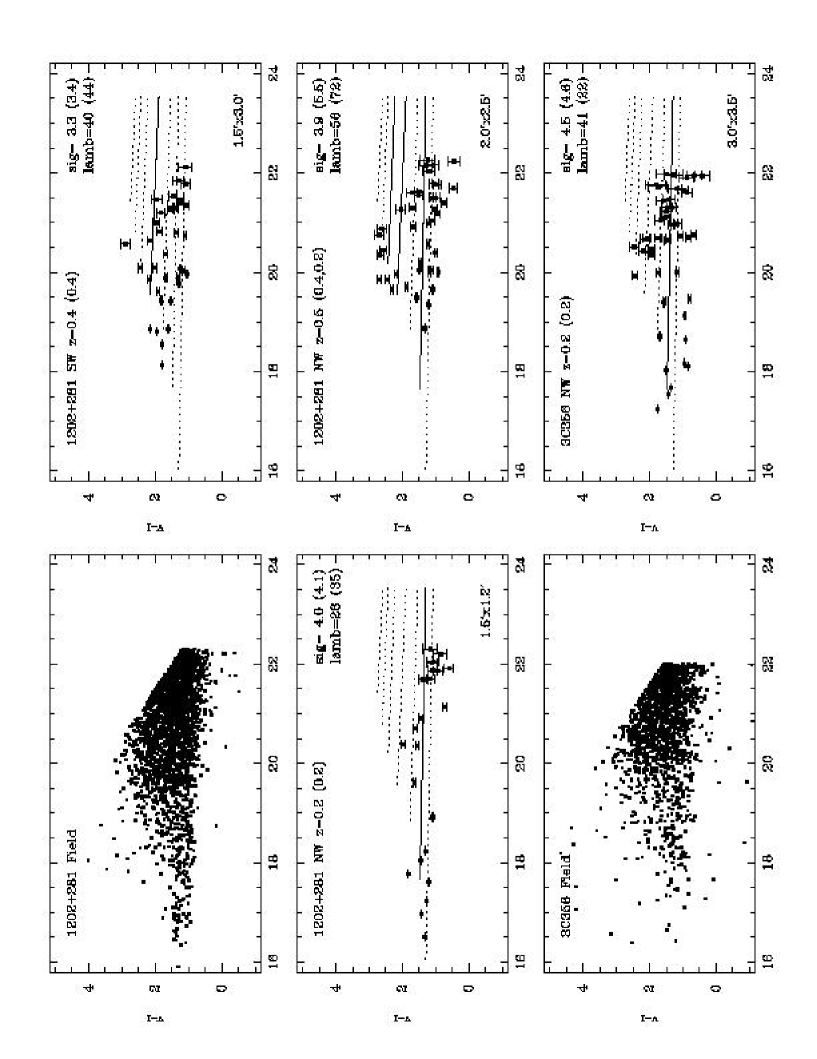
Figure 12: V-I vs. I distributions for mutual V and I cluster candidates in 1202+281 ROSAT field and for 1 of the 2 candidates in the 3C356 ROSAT field. The solid line(s) plot the sequence at the estimated redshift(s) of the cluster candidates. The dashed lines show the red sequences predicted for $z=0.1-0.7$ in increments of $\Delta z=0.1$. The upper left label indicates the field, the quadrant, the estimated redshift from the I(V). The upper right label lists the detection confidence (sig) in I(V), and $\Lambda_{cl}$ (lamb) from the I(V) data. Lower right label lists the cluster core size.

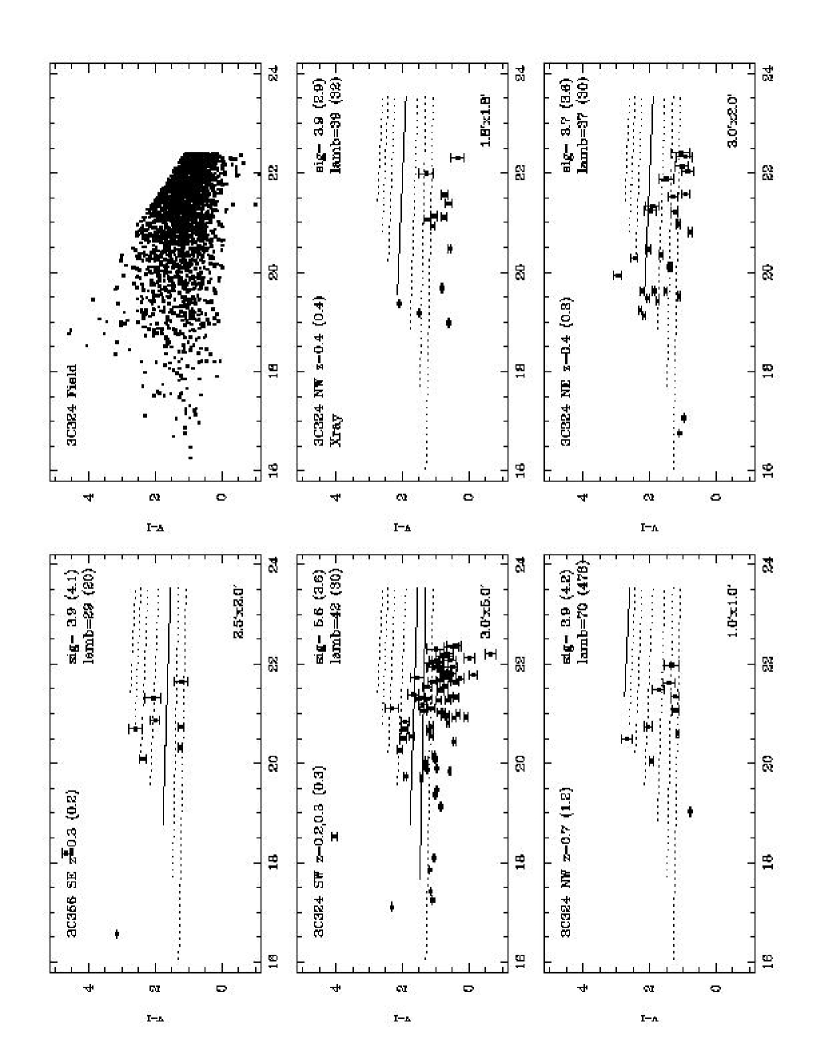
Figure 13: V-I vs. I distributions for mutual V and I cluster candidates in the 3C356 (1 of 2) and 3C324 ROSAT fields. Plots are annotated as in Figure 12.

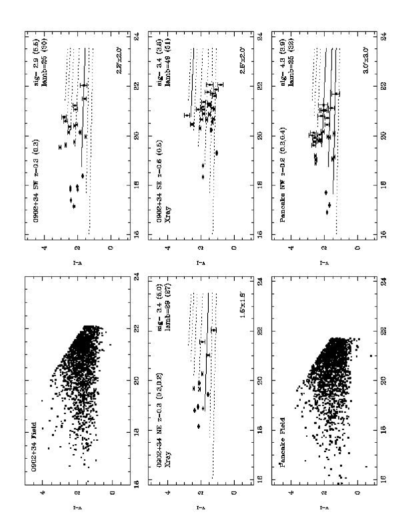
Figure 14: V-I vs. I distributions for mutual V and I cluster candidates in the Zel’dovich Pancake and the 0902+34 ROSAT fields. Plots are annotated as in Figure 12.

In Figures 12-15, we present the galaxy color-magnitude diagrams for the background galaxies and the candidate clusters, along with the size of the cluster aperture, the estimated redshifts from the I (V) band data, the optical detection significance in I (V), and the corresponding value of $\Lambda_{cl}$ in I (V). We overplot the color magnitude relations for 7 different redshifts between $z=0.1-0.7$, corrected to the Landolt (1992) system (Johnson V and Cousins I) from the AB V and I magnitudes used in Gladders & Yee (2000). The darkest line represents the estimated redshift from the matched filter output for the V and I data. The uncertainties in I and V-I are relatively small for $I<22$ - over a magnitude above our completeness limit, so we are confident that our photometry is sufficiently deep and accurate to show a red sequence at least for clusters with $z<0.7-0.8$. However, visual inspection shows that very few of the clusters has a particularly strong red sequence - even the confirmed X-ray clusters have fewer than 10 galaxies near the expected red sequence lines.

To quantify statistically our visual assessment of the color-magnitude plots, we constructed a two-dimensional two-sample Kolmogorov Smirnov test (Press et al. 1997) in order to estimate the probability that the photometric V-I and I values of the possible cluster galaxies and the field galaxies were simply drawn from the same parent distribution. We list the results in Table 3, for all cluster candidates where analysis was possible. For each field we list the number of galaxies in the field population, typically $\sim 2000$ galaxies in each. The column $N_{gals}$ lists the numbers of galaxies in the cluster candidate sample and the column $P(KS)$ contains the probability that the V-I and I values in the cluster candidate sample were randomly drawn from the same parent population as the field galaxies, as plotted in the first panel for each of the 5 ROSAT fields. Only 7 out of the 16 I-band cluster candidates showed a KS probability lower than 2%. The K-S test is not a test of the presence of a red sequence; but a lack of a significant K-S result for over 50% of these candidates, including 50% of the candidates with X-ray counterparts, reflects the qualitative difficulty of discerning a red sequence in these data. One of the 5 X-ray candidates had only limited galaxy photometry data; 2 of the remaining 4 X-ray candidates had high and thus insignificant K-S probabilities distinguishing the colors and magnitudes of galaxies in the core from those of background galaxies. The result of the K-S test confirms our sense that not many of the cluster candidates exhibit a strong red sequence on the color-magnitude plots.

This result suggests that for many of the ROXS candidates with both a V and an I detection, a red sequence is not particularly prominent, even for cluster candidates where both I and V-band counterparts exist nearby an X-ray cluster candidate. If these candidates are true clusters – and it seems unlikely that these triply-identified candidates are spurious – this result implies that searches for a prominent red sequence may miss clusters of galaxies at any given redshift, at least at the mass scales sampled by this survey. The red-sequence method and its creators do not claim to create a sample of clusters with galaxy populations representative of all clusters at a given redshift, since the method selects clusters by their old galaxy populations. (Furthermore, the red sequence method may not require a prominent red sequence.) Therefore the ROXS result may not be surprising since none of the ROXS candidates are particularly X-ray luminous. The observed 0.5-2.0 keV X-ray luminosities of the X-ray candidates with V and I counterparts lie between $3-70\times 10^{42}h_{75}^{-2}$ erg s^-1, which places them in the category of richness class 0 clusters and even groups; we note however that the estimated $\Lambda_{cl}$ for these cluster candidates are as high as 70-85, not particularly consistent with groups.

A prominent red sequence may preferentially exist in the most X-ray luminous clusters and groups, which are the most likely to be dominated by elliptical galaxies in their cores. X-ray luminous groups with central ellipticals and prominent elliptical galaxy populations are more X-ray luminous than their spiral-dominated counterparts (Mulchaey & Zabludoff 1998). Since the ROXS cluster candidates are not very X-ray luminous (whether they were detected in the X-ray or not), they might have a higher spiral component and are more like the Virgo cluster ($L_{x}\sim 10^{43}{\rm erg\,s^{-1}}$) than they are like Coma ($L_{x}\sim 10^{44}{\rm erg\,s^{-1}}$). Stanford, Eisenhardt & Dickinson (1998; SED98) looked at various properties of the color-magnitude relation for early-type galaxies in high-redshift clusters, including the scatter of those properties, and found that for most of the SED98 clusters there was little variation in either the properties or their scatter. However, all of the SED98 clusters are more luminous than the ROXS clusters in our color-magnitude study. Therefore if the explanation for the ROXS results is that there is an X-ray luminosity threshold below which the color-magnitude properties break down, the SED98 study would not have seen it. A red sequence may be the most distinct at the highest masses and at the lowest redshifts, but at present it is uncertain at what mass and at what redshift the sequence may begin to be indistinct and difficult to see in clusters.

5.6 Simulations of ROX

In Paper I, we produced a $\Lambda_{cl}$ function based on our data and, using the $L_{x}-\Lambda_{cl}$ relation, we compared that function to the X-ray luminosity function for clusters of galaxies. We found that a steep $L_{x}-\Lambda$ relation (steeper than the predicted $L_{x}\propto\Lambda_{cl}^{2}$) was needed to explain the observed X-ray and optical luminosity functions for the ROXS clusters. The proportionality, $L_{x}\propto\Lambda^{2}$ derives from the observed $L_{x}\propto T_{x}^{3}$ relation for clusters, an assumption of a constant $M/L$ ratio for clusters, and $T_{x}\propto M^{2/3}$ from hydrodynamics simulations. We also demonstrated in Paper I that unless our observation errors are underestimated, the scatter in the observed $L_{x}-\Lambda$ relation is large and intrinsic.

We have performed a numerical simulation of the ROXS, accounting for all major selection and measurement effects. We confirm the basic empirical results, namely that the instrinsic cluster population must have both a moderately steep richness to X-ray-luminosity relationship and significant physical scatter between richness and X-ray luminosity in order to reproduce the survey results. In this section we briefly describe the simulation methodology and analysis.

Using Monte-Carlo techniques we first generate a large X-ray cluster population ($5\times 10^{4}$ members) occupying a volume from $z=0$ to $z=2$. We draw members according to the local X-ray luminosity function (0.1-2.4 keV) of Ebeling et al (1997), which we assume to be unevolving with $z$. Current constraints show at most weak (less than 10%) evolution in the cluster population to redshifts of at least $z=0.5$ (cf. Gioia et al 2001; Lewis et al. 2002). Since ultimately very few clusters will be selected at $z>1$ by the ROXS criteria we consider a non-evolving X-ray luminosity function to be a valid assumption for our first-order goals.

Assuming a optical to X-ray luminosity relationship of the form $\Lambda=AL_{x}^{\alpha}$ and an instrinsic scatter expressed by a normally distributed random variable $\Delta A$ where the amplitude is either fixed or a fractional value of $A$, we assign a $\Lambda$ to each cluster. Via a Monte-Carlo approach we then sample this cluster population and apply both the X-ray selection criteria and optical selection criteria of the ROXS until a total of $N$ clusters have been “observed”. The X-ray detection criteria are slightly complicated by the known dependency on the combination of cluster angular extent and net flux. Using an empirical relationship between cluster luminosity and X-ray core radius (assuming a standard King profile for cluster density) of: $r_{c}=0.125(L_{x}$h${}^{-2}/1.25\times 10^{44}~{}{\rm erg\,s^{-1}})^{0.2}$ Mpc h^-1 (Jones et al 1998), we derive the angular size of the X-ray cluster. The X-ray selection functions for the simulation are essentially the same as the X-ray selection functions in Figure 3 in § 4, except for the simplifying notion that all clusters were observed on-axis by the ROSAT PSPC. Cluster luminosities are converted to the X-ray detection band (0.5-2 keV) assuming a constant 4 keV thermal spectrum, which is a reasonable approximation for our observed sample.

Clusters are entirely discarded which fall outside of the $0.2<z<1.2$ range of the ROXS. Clusters which are only detected in either the X-ray or optical, but not both, are flagged. Those detected only in the optical are then assigned an X-ray flux upper-limit (and X-ray luminosity upper limit) based on the mean X-ray flux limit of the ROXS ($\sim 10^{-14}$ erg s^-1 cm^-2 0.5-2 keV). Finally, the $\Lambda_{cl}$ for each cluster is assigned an observational error as a function of redshift, based on the known error distributions of the matched-filter algorithm, which correspond to $\sim 10$% errors for $z<0.7$ and $\sim 50$% errors for $z>1$ (P96).

We are therefore left with four datasets: joint X-ray and optical detected clusters, optically detected clusters with X-ray upper limits, X-ray detected but not optically detected clusters, and entirely undetected clusters.

In Figure 16 we plot the results for a simulated dataset where $L_{x}\propto\Lambda^{2}$ (the fiducial relationship expected under basic assumptions) and that the $\Lambda-L_{x}$ scatter is zero. Observational errors are still included in $\Lambda$, so some spread is still seen. The total number of systems is arbitrary, but chosen here for clarity of presentation. It is immediately apparent that this particular simulation does not qualitatively agree with the observations, both in the shallowness of the relation and in the scatter between $L_{x}$ and $\Lambda$. The relative numbers of joint, only optical, or only X-ray detections are also in strong disagreement with observations. We observe approximately 4 cluster candidates in the ROXS which are only detected optically for every 1 cluster which is jointly detected, and no more than 3% of all candidates are solely X-ray candidates. In the simulation of Figure 16 the mean numbers of detections (over 10 runs) yields a straight 1:1 ratio between jointly detected and optically detected clusters, at odds with the real ROXS, although the fraction of the purely X-ray detected numbers are consistent and are at about the 3% level. Adding a significant intrinsic scatter ($1\sigma=$28% of the normalization $A$) to the $L_{x}-\Lambda$ relationship does not alter these results.

In contrast, in Figure 17 we plot the results for $L_{x}\propto\Lambda^{3}$ and an intrinsic scatter of $1\sigma=$39%. It is apparent that there is much better qualitative agreement between this simulation and the ROXS results. Furthermore, the relative numbers of X-ray vs. optical cluster detections are now in much better agreement. The simulation yields a 4 to 1 ratio for optical detections vs joint detections, and a pure X-ray detection rate of 1-2%.

Interestingly, a steeper relationship ($L_{x}\propto\Lambda^{4}$) appears to be less successful at reproducing the ROXS observations, even when we adjust the allowed scatter. Typically, the number of optical-only detections are overproduced by at least a factor of 2 in such tests.

We note here that the simulations are seriously limited in their ability to provide a faithful reproduction of the actual ROXS data. This limitation is for a variety of reasons. Without much greater complexity we cannot mimic the details of the X-ray selection, namely the variation in detection sensitivity as a function of off-axis position in the ROSAT fields, and the detailed variations in field exposure times and backgrounds. We are also reliant on the $\Lambda$ selection functions, which are known to suffer increasing uncertainties with $z$. The basic findings are however clear. The $\L_{x}-\Lambda$ relationship must be steeper than $\Lambda^{2}$, and the intrinsic scatter between $L_{x}$ and $\Lambda$ must be large - these are not due to systematics in the observations.

A somewhat more quantitative evaluation of the simulation results is summarized in Figure 18. We have applied a 2D K-S test (Press et al 1997) to the ROXS joint detections (X-ray and optically detected clusters) and the equivalent simulation outputs for a range of parameters in the $\Lambda=AL_{x}^{\alpha}$ relation. Specifically, we have chosen a fixed instrinsic fractional dispersion in this relation such that the $1\sigma$ width is 100% when the normalization $A$ is 50 and approximately 30% when $A=175$. We have then varied $A$ and set $\alpha$ to $1/2$, $1/3$ and $1/4$. In Figure 18 (upper panel) we plot the resultant 2D K-S probabilities. These should be considered only in relation to each other rather than as absolute indicators of a ‘goodness-of-fit’. The higher the probability the more significant the agreement between distributions. It is apparent that when $\alpha=1/2$ the agreement between the ROXS and the simulations is never very good, but does seem to peak around $A=100$. In constrast, for $\alpha\leq 1/3$, the agreement appears best for low $A$, comparable to $\alpha=1/2$ for $a\simeq 100$ and significantly worse for $A>120$. Variations as large as 50% in the intrinsic scatter used in the simulations do not significantly alter these results.

However, as described above, visual inspection of the data in the $L_{x}-\Lambda$ panel reveals that the 2D K-S test may be somewhat misleading, and in fact neither the low-$\alpha$ results at low $A$ or the $\alpha=1/2$ results at $a\sim 100$ would be classed as very good fits ‘by-eye’. For example, when $\alpha=1/2$ the simulated and observed distributions overlap only at the lower $L_{x}$ end, which boosts the K-S probability relative to $\alpha=1/3$, although the latter distribution is better aligned, its overlap is smaller.

The situation is considerably clearer when we also take into account the number ratios of joint detections versus optical only detections (as discussed above). In Figure 18 (lower panel) we plot the ratio of the number of joint detections to the number of optical-only detections for the 3 cases described above. We also plot the actual ROXS ratio (dashed line). It is immediately apparent that only the $\alpha=1/3-1/4$ curves intersect the observations for reasonable $A$. Weighing the 2D K-S results by this additional constraint we conclude that the simulations are in best agreement with the data when $\alpha\simeq 1/3-1/4$ (since the KS probabilities are overall higher) and when $A\simeq 100-150$. $L_{x}\propto\Lambda^{2}$ is therefore excluded as a plausible intrinsic relationship.

6 Discussion

The optical matched-filter selection technique works well to find candidate clusters of galaxies, but the spurious fraction is high at $\sim 30\%$, and it is demonstrably not 100% complete - it misses clusters at a rate of 10-20% at least. The selection window for a matched filter cluster sample is more difficult to quantify because of its sensitivity to the spectral energy distribution of the galaxies for which it is searching.

On the other hand, the X-ray selection technique, while generating fewer spurious cluster candidates ($\sim 10\%$) and reliably finding the (apparently) more massive clusters, misses some high $\Lambda_{cl}$ cluster candidates. We do not know yet whether these are true massive clusters or whether they are fortuitous projections of less massive systems. Redshifts and X-ray observations are required to determine the nature of these candidates. Zabludoff & Mulchaey (1998) and Mulchaey & Zabludoff (1998) showed in their sample of 12 optically selected groups that groups without detected X-ray emission tend to be lower velocity dispersion systems with few or no elliptical galaxies. The undetected groups in the Zabludoff & Mulchaey sample may not even be bound. Some X-ray observations of optically-selected, high redshift clusters have revealed such clusters to be “underluminous” in the X-ray (Castander et al 1994.) The high-significance, optically rich ROXS candidates without X-ray counterparts are prime targets for observational tests whether X-ray selection indeed selects on the basis of cluster mass. The correlation of the presence of a dense, X-ray emitting intracluster media and the presence of a significant elliptical galaxy population is another testable hypothesis with further observations of the ROXS sample. With the limited color information we have in hand, we were not able to show that X-ray cluster candidates at the moderate X-ray luminosity levels available in our sample are more likely to have red elliptical sequences. But we were only able to make this test for a small number of cluster candidates, given the available photometry.

A related result from ROXS is that the cluster richness $N_{R}$ is not well-correlated with cluster X-ray luminosity, a result which is supplementary to our result in Paper I regarding cluster X-ray luminosity and the $\Lambda_{cl}$ richness parameter. The clusters in our sample are on average poorer and less massive than those found in a half-sky survey (e.g. XBACS), owing to the smaller sky area and greater depth of our survey. For $\Lambda>30$, Donahue et al. (2001) suggested that the joint redshift and $\Lambda_{cl}$ distribution arises from the population of X-ray clusters with a steep dependence between $L_{x}$ and $\Lambda_{cl}$. Equivalently, we show here that we can also reproduce this joint distribution with a large scatter between $L_{x}$ and $\Lambda_{cl}$ in Monte-Carlo simulations of the ROXS.

A correlation between cluster X-ray luminosity and cluster richness has been suspected at least since Jones & Forman (1978) plotted cluster richness class against X-ray luminosity for nearby ($z<0.07$) clusters. But even in their sample, a $3\times 10^{44}~{}{\rm erg\,s^{-1}}$ cluster is equally as likely to have a cluster richness of 0 as it is 2 or 3. Only the most luminous clusters ($L_{x}>10^{45}~{}{\rm erg\,s^{-1}}$) had cluster richnesses reliably of 2 or 3. The XBACS clusters (Figure 7) show this correlation and very large scatter with cluster richness. However, richness has long been a suspect observational parameter for X-ray astronomers (e.g. Mushotzky et al 1978), since the measurements rely on number counts that only become more difficult to ascertain at higher redshift with the associated higher contamination levels. The matched filter method provides a possibly more robust and objective means of estimating a cluster candidate’s luminosity in the form of $\Lambda_{cl}$, yet, this measure too is not strongly correlated with cluster X-ray luminosity.

The lack of strong correlation between X-ray and optical luminosity, and the large scatter of those two quantities, are confirmed by the ROX Survey. A review by Borgani & Guzzo (2001) showed that the velocity dispersions and cluster optical luminosities of an optically-selected sample of clusters are not as well-correlated as the velocity dispersions and the optical luminosities of a subsample of clusters selected for their X-ray fluxes from the original sample. The velocity dispersions of these X-ray selected clusters are even better correlated with their X-ray luminosities, suggesting that X-ray luminosity is better correlated with cluster mass than is optical luminosity. The ROX Survey has no such independent test of correlation with mass; however, followup observations of this sample in the X-ray and the optical will further test the Borgani & Guzzo suggestion at higher redshifts.

The ROXS, since it is a uniformly selected sample at both X-ray and optical wavelengths, has examples of both X-ray candidates without optical counterparts and optical candidates without X-ray counterparts. Both subsamples probe the extremes of the $L_{x}/L_{opt}$ distribution. Explaining the extremes will go a long way towards explaining why and how the emissivity of the intracluster gas is related to the light emitted by the stars in the cluster. It is particularly important to see if there is a “third parameter” such as galaxy formation efficiency, evolutionary stage of the cluster, or galaxy morphology populations, that creates the large spread in the $L_{x}$ versus richness relationship for clusters, or if the large spread is due to projection effects significantly impacting the optical selection technique. One possible clue is the existence of a difference in the conclusions based on cluster contents from an optically-selected, rather heterogenous sample of clusters (the MORPHS sample, in Smail et al 1997) and those found in an X-ray selected sample of clusters by Ellingson et al (2001). The X-ray selected clusters show cores that exhibit very little evolution between $z=0.5$ and the present, whereas the MORPHS clusters show evidence that the S0 population may be turning into ellipticals during that same time. It is possible that the presence of a well-developed intracluster medium is ubiquitous in a massive cluster, but in less massive clusters, the galaxy populations are still evolving in the cluster cores. Uniform morphological studies of a cluster sample diverse in X-ray and optical properties are needed to test such a statement, and such a test could be accomplished with a sample such as the ROXS.

Rosati et al. (1995, 1998) selected clusters for the RDCS not only for their X-ray emission, but used an extent criteria as well. There was some worry that this selection criteria may have missed the most compact X-ray clusters which remain unresolved by the ROSAT PSPC, particularly those at high redshift. However, our survey does not reveal an obvious population of high redshift cluster candidates with X-ray point sources. The correspondence between an optical cluster and an X-ray point source is not more than we would expect by chance - therefore we do not believe we have found a population of cluster sources which would go undetected by the ROSAT cluster surveys which select for extent, a result consistent with the findings of the Wide Angle ROSAT Pointed Survey (WARPS; Jones et al 1998), a ROSAT serendipitous search which did not filter for extent. We have some examples of optical clusters with X-ray point source counterparts which could be AGN in those clusters. Approximately 25 of our candidates have X-ray point sources within 1’-2’ of the cluster centroid; optical identification of these sources is required to ascertain whether the candidate and the point source are physically related.

Probably the most surprising result is that the ROXS cluster candidates do not, as a rule, show distinct or strong red sequences in the color-magnitude diagrams of their galaxy populations. Only about 50% of the optical cluster candidates detected in both I- and V-band show galaxy colors distinct from those of the field population. And only $\sim 50\%$ of the X-ray clusters so identified show such sequences. It is possible that the red sequence is ubiquitous in the most massive, virialized clusters. But perhaps at some unknown threshold in mass or level of virialization or luminosity, the red sequence ceases to be distinct and prominent. We plan to use the red sequence detection method (Gladders & Yee 2000), which does not rely on an obvious red sequence to select cluster candidates, to see what cluster candidates it finds in the ROXS galaxy photometry data.

The ROXS sample identifies several problems that warrant further investigation:

• A red sequence is not prominent in all X-ray selected clusters. At what X-ray luminosity (or equivalently at what mass) does the red sequence cease to be prominent? Is the presence of a red sequence dependent on mass?

• The estimated optical luminosity and richness of a cluster are not at all well-correlated with the X-ray luminosity. There are at least three unsolved issues regarding the correlation of the optical luminosity, X-ray luminosity, and cluster virial mass:

  1. Is the lack of correlation representative of the difficulties of estimating the optical luminosity or is it representative of an intrinsic variation or scatter in the M/L ratios in clusters?

  2. If the estimated optical or X-ray luminosity, and therefore the detectability of a cluster, has enormous scatter with respect to the mass of the cluster, selection by mass using optical or X-ray light may be very difficult. Knowing the scatter with respect to cluster mass with both optical and X-ray luminosity is important. Individual studies show good correspondence of both quantities with velocity dispersion (e.g. Girardi et al. 2000 and Mahdavi & Geller 2001 for $L_{B}$ and $L_{x}$ respectively), but a comparative analysis of the masses and luminosities of a well-chosen, homogeneous sample has not been done yet.

  3. If there is such a large intrinsic variation in the optical M/L for clusters, what evolutionary process controls this variation? Can galaxy formation efficiency or evolutionary history be so radically different from one cluster environment to another to produce this effect? Does M/L correlate with any other property of a cluster of galaxies?

• While galaxies and hot gas may trace the gravitational potentials of the most massive clusters, mergers and other physics may disrupt that correspondence. True optical condensations of galaxies with low levels of X-ray emission may be galaxies which have been temporarily separated from the hot intracluster gas while undergoing a merger event; galaxies experience the merger as a non-collisional fluid while the gas experiences hydrodynamic effects of shocks and cooling. An observational example of such a merger is Abell 754 (Zabludoff & Zaritsky 1995). Studies of the ROXS “X-ray poor” cluster candidates may reveal their true nature, whether they are mergers, minor systems embedded in filaments, or mere projection effects.

Because the ROXS has greater depth and smaller sky area than surveys like the EMSS or XBACS, the ROXS clusters must be relatively low-mass clusters compared to typical clusters in those surveys. The low-mass end of the cluster mass function may be where the physics of the intracluster medium collides with the physics of star formation and galactic winds. The energy injected by stellar processes is closer to the specific energy per particle in the gravitationally bound gas of a low mass cluster of galaxies. Mergers may be more common or at least more significant in the low-mass clusters – when the relative velocities of the galaxies are not much greater than the internal velocities of the galaxies, collisions and interactions are more likely to induce star formation. The least massive clusters may be the most recent members to the cluster hierarchy, whose galaxies are most recently accreted from the field. The optical and X-ray properties of such clusters may thus still be correlated, but only very weakly and with high scatter. Such recent formation may explain the weakness or lack of a red sequence, which may only dominate in clusters where the oldest ellipticals formed preferentially in high density regions at an early time. The other inference possible from ROXS is that at some point below a given mass on the mass scale of clusters, some treasured assumptions about clusters, their M/L constancy, the invariance of the baryon fraction in clusters, and their ubiquitous red galaxy content may break down.

7 Summary

No single cluster selection method is perfect. Multiple, complementary methods of selecting clusters may be essential for cluster studies, particularly at high redshift where all methods start to run into completeness limits, incomplete understanding of physical evolution, and projection effects. Understanding the biases inherent in any cluster selection method is essential to extracting conclusions about cluster evolution or the evolution of galaxies in clusters from any cluster sample. The ROSAT Optical X-ray Survey (ROXS) for clusters of galaxies provides a well-matched, head-to-head comparison of two of the most popular methods for finding clusters of galaxies: a matched filter in the optical and extended source detection algorithms such as the wavelet transform in the X-ray. Both algorithms do seem to agree on the location of at least some of the cluster candidates in our sky coverage; however, the overlap was far from perfect.

We find that the correlation is weak between the X-ray and optical luminosity or richness of a cluster, and it has considerable intrinsic scatter. Some of this scatter may arise from underestimating our observational uncertainties, but the scatter is too large for it to be accounted for by pure observational uncertainties in $L_{x}$ or $\Lambda_{cl}$ (Paper I). We confirm these results in a numerical model of the ROXS. While we did not find any bias that would affect the conclusions on the evolution of clusters of galaxies, we did find evidence for possible bias that could affect conclusions regarding galaxy evolution in clusters. X-ray and optical cluster detection techniques sample different cluster populations, a statement which should worry those who use cluster samples to make claims about galaxy evolution.

We find that the red-sequence does not appear to be very strong in our cluster candidates, regardless of whether they have X-ray counterparts. We plan to do a proper red sequence detection with the ROXS galaxy photometry and position data in an upcoming paper.

All cluster methods have their merits; the cluster community should consider, however, the effect of cluster selection and the measurement of cluster properties on their conclusions. The ROXS has provided a number of follow-up avenues to assess in detail the real differences between cluster candidates which were detected in the X-ray and those which were not. Observations to obtain the weak lensing signatures, velocity dispersions, and/or ICM temperatures would provide the most fundamental property of a cluster from a cosmologist’s perspective - its virial mass. Confirmation of at least a subsample of the optical clusters with the faintest X-ray limits would more strongly test our working hypothesis that we have no need to invoke the presence a bi-modal population of X-ray faint and X-ray luminous clusters of galaxies at the mass scales of $10^{14}-10^{15}~{}\rm{M}_{\odot}$. Clusters whose X-ray/optical luminosities lie outside the normal distribution could reveal clusters in early evolutionary states or clusters embedded in unusual projection with respect to filaments and other large scale structure, or they may represent a fundamental challenge to our assumptions about cluster physics and formation.

Figure 1: The optical matched filter detection probabilities in the I-band as a function of redshift for systems of richness $\Lambda=$30, 50, 100, 200, 300 (in order of increasing line weight). The probabilities were determined using the methods of P96.

Figure 2: Mean number of extended and pointlike X-ray sources per unit area as a function of distance from the center of the ROSAT field.

Figure 3: The X-ray detection probability in the 0.5-2 keV band as a function of redshift for intrinsic X-ray luminosities (0.5-2 keV) of 0.01, 0.1, 1.0, 5.0 and 10 $\times 10^{44}$erg s^-1 ($H_{0}=75$, $q_{0}=0.5$) (in order of increasing line weight, from left to right). The detection probability is plotted as the net probability over all 23 ROXS fields, based on exposure time, background surface brightness, and radial detection efficiency due to PSF variations for a cluster with a given X-ray luminosity and redshift and a standard radial surface profile (Jones et al. 1998) and $\beta=2/3$ (Scharf et al. 1997; Rosati et al. 1995).

Figure 5: The black line shows the distribution of the upper limits to the bolometric X-ray luminosities of the cluster candidates which were not detected in the X-ray. The dashed lines show the distribution of the optical cluster candidates which were cross-identified with X-ray sources. The lower luminosity candidates and optical candidates with low luminosity upper limits lie at low estimated redshifts $z\sim 0.2-0.3$.

Figure 7: X-ray luminosities vs. optical richness for XBACS clusters (open circles, both panels) and ROXS optical cluster candidates with X-ray counterparts (filled circles, left panel) and the upper limits on the X-ray luminosity for ROXS optical candidates without X-ray counterparts (filled triangles, right panel). The size of the error bars for the ROXS optical richness reflects the uncertainty in the conversion from $\Lambda_{cl}$, the matched filter optical luminosity parameter, to $N_{R}$, optical richness.

Figure 8: The redshift (left) and $\Lambda_{cl}$ (right) histograms of all 155 optically selected cluster candidates, of which 3 have $<2.9\sigma$. The dotted line indicates those clusters with X-ray counterparts. The dashed line indicates the histogram of candidates with X-ray counterparts and optical candidates deemed “probable” in a subjective assessment.

Figure 9: The distribution of aperture-corrected $\Lambda_{cl}(1+z^{9})^{0.7}$ (correction from P96), with the same line codes as Figure 8. The majority of the optically selected cluster candidates with corrected $\Lambda_{cl}>100$ have estimated $z>1$, and are not probable clusters, according to our subjective assessment.

Figure 10: The distribution of the optical detection confidence in units of $\sigma$ for all of the optical candidates is plotted in a solid line. The same distribution for the X-ray/optical cross-identifications is plotted with a dotted line. Those clusters which were additionally identified as “likely” clusters are shown in a dashed line. Note that the majority of the X-ray/optical clusters lie in the bin with detection significance 3-4$\sigma$.

Figure 11: The optical detection confidence is plotted here against $\Lambda_{cl}$, an estimate of the cluster’s optical luminosity. The two quantities are not strongly correlated.

Figure 15: V-I vs. I distributions for 3 mutual V and I cluster candidates in Zel’dovich Pancake ROSAT field. Plots are annotated as in Figure 12.

Figure 16: $L_{x}$ vs. $\Lambda$ is plotted for the three cluster detection datasets in a ROXS simulation with $L_{x}\propto\Lambda^{2}$, normalized to approximate the observed relationship. Leftmost panel plots clusters jointly detected in the X-ray and optical, point size is proportional to cluster redshift ($0.2<z<1.2$). Solid curve is the $L_{x}\propto\Lambda^{2}$ relationship used to generate the clusters, dashed curve is an $L_{x}\propto\Lambda^{4}$ relationship. Center plot is of X-ray upper limits for clusters only detected optically. Note that since these are $4\sigma$ upper limits to $L_{x}$ and the clusters are typically at higher $z$ for a given $\Lambda$ than the detected systems, these points occupy a region above the instrinsic curve. Rightmost panel plots those clusters which are X-ray detected but not optically detected (1 object in this simulation). $L_{x}$ is in units $10^{44}{\rm erg\,s^{-1}}$.

Figure 17: As for Figure 16, but simulation now uses $L_{x}\propto\Lambda^{3}$ and an instrinsic scatter with $1\sigma=$39% of the amplitude.

Figure 18: Summary of 2D K-S test and simulation results. In the upper panel the 2D K-S probabilities (of a significant match between the ROXS joint X-ray/optical detection $\Lambda$, $L_{x}$ data and the simulation joint detections) are plotted as a function of the normalization $A$ in the simulation $\Lambda=AL_{x}^{\alpha}$ relationship. Simulation data is taken from single Monte Carlo runs which generate at least 50 joint detection data points, scatter between runs is small compared to the true variations in these curves. Lightest curve is for $\alpha=1/2$, medium is $\alpha=1/3$, and the heaviest is $\alpha=1/4$. Lower panel shows the number ratio of jointly detected clusters to those only detected optically, curves are as for the upper panel. The dashed horizontal line denotes the observed ratio for the ROXS.

Table 1: ROSAT fields

ROSAT Field	ROSAT Target	ROSAT Exptime	RA	Dec	Area	KPNO Date
		(sec)	J2000	J2000	deg2	I-Band	V-Band
RP700112	MKN 78	19844	07:42:40	65:10:52	0.17518	03/18/96
RP700326N00	0902+34	14355	09:05:31	34:07:48	0.24414	03/17/96	05/06/97
RP900327	Zeldovich Pancake	55611	09:06:52	33:40:16	0.24161	03/16/96	03/18/96
WP700540	10214+4724	19359	10:24:33	47:09:04	0.24401	03/17/96
WP201243N00	PG1034+001	18111	10:37:05	-00:08:21	0.19623	05/09/97
WP700228	1116+215	24585	11:19:09	21:19:16	0.24343	03/17/96
WP201367M01	PG1159-035	32219	12:04:25	-03:40:16	0.23667	03/18/96
WP700232	1202+281	27859	12:04:43	27:54:04	0.23531	03/18/96	05/06/97
RP700864A01	3C 270.1	19290	12:20:33	33:43:16	0.19836	05/06/97
RP600242A01	Giovanelli-Haynes Cl	24830	12:27:43	01:36:04	0.18036	05/08/97
RP700073	3C 280	48051	12:56:57	47:20:28	0.16501	03/17/96
RP700216A00	B2 1308+32	8316	13:10:29	32:20:59	0.19679	05/09/97
RP700117	3CR294	22692	14:06:43	34:11:27	0.19156	05/07/97
WP700248	1411+442	25319	14:13:48	44:00:04	0.23088	03/16/96
RP700122	Q1413+1143	28066	14:15:45	11:29:46	0.24770	03/18/96
RP800401A01	4C23.37	11811	14:15:58	23:07:12	0.23037	03/16/96
RP700257N00	MKN 841	16842	15:04:02	10:26:24	0.18221	05/09/97
RP701373N00	3C 324	15434	15:49:50	21:25:52	0.22442	03/17/96	05/06/97
RP800239N00	CL1603	28763	16:04:29	43:13:12	0.18933	05/08/97
RP300021N00	MS1603.6+2600	24506	16:05:46	25:51:36	0.19376	05/08/97
WP170154	WFC/PSPC Calibr	37490	16:29:32	78:04:52	0.18426	05/09/97
701457n00	HS1700+6416	27408	17:01:00	64:11:59	0.18889	05/08/97
RP800395N00	3C 356	18563	17:24:19	50:57:36	0.22243	03/18/96	05/06/97

Table 2: Optical Cluster Candidates

Optical ID	RA	Dec	Sigma	Lambda	z	I-mag	Radius	Theta	Flim 1’	Xray Match	Comment
							(”)	(’)	(10-14)
RP700112 - MKN 78
OC1 0740+6504	07 40 57.25	65 04 00.9	3.42	31.17	0.30	19.46	138	12.85	1.9
OC2 0741+6524	07 41 44.06	65 24 42.9	3.25	38.69	0.40	20.29	162	15.11	2.1		PtSource within 30”
OC2a 0742+6519	07 42 14.19	65 19 43.7	3.31	30.13	0.30	19.60	170	9.35	1.7
OC3 0743+6458	07 43 45.82	64 58 14.9	5.45	64.88	0.40	20.13	162	14.31	2.1	RXJ0743.7+6457	Cluster within 1’
RP700326N00 - 0902+34
OC1 0904+3411	09 04 23.88	34 11 04.9	4.25	43.38	0.40	20.13	70	14.27	2.5		Edge,Compact
OC2 0905+3359	09 05 10.18	33 59 37.6	2.94	25.04	0.30	19.24	59	9.24	2.1		Compact,Low Sig
OC3 0905+3421	09 05 11.11	34 21 53.0	5.14	34.79	0.20	18.39	116	14.67	2.5		Edge,Pt Source within 1’
OC4 0905+3403	09 05 52.95	34 03 17.5	3.58	88.98	1.00	22.51	101	6.40	1.8		Blend OC5?
OC5 0905+3407	09 05 57.01	34 07 00.6	3.35	48.56	0.60	21.28	177	5.44	1.8		Blend OC7 and OC4?
OC6 0906+3417	09 06 17.59	34 17 16.0	3.39	28.87	0.30	19.24	79	13.50	1.8	RXJ0906.3+3417	Cluster within 15”
OC7 0906+3405	09 06 28.25	34 05 11.9	5.40	36.56	0.20	18.39	275	12.13	2.4		PtSource within 2.0’
OC8 0906+3359	09 06 31.74	33 59 51.1	4.05	70.13	0.70	21.65	165	14.89	2.3		PtSource within 1.5’, blend OC7?
OC9 0906+3413	09 06 32.70	34 13 17.4	3.35	89.67	1.10	22.71	50	13.88	2.5
RP900327 - Zel’dovich Pancake
OC1 0906+3354	09 06 12.55	33 54 21.9	4.32	25.13	0.20	18.10	227	16.45	1.7
OC2 0907+3330	09 07 18.64	33 30 44.5	5.23	85.19	0.50	20.71	174	10.88	1.3	RXJ0907.3+3330	Cluster within 30”
OC3 0907+3343	09 07 27.69	33 43 02.5	4.59	74.79	0.50	20.85	268	7.80	1.0	RXJ0907.4+3342	Cluster within 30”
OC4 0907+3355	09 07 47.16	33 55 00.4	3.50	28.21	0.30	19.47	68	18.62	1.9		Edge,Compact,Near cut area
OC5 0907+3350	09 07 58.29	33 50 09.6	3.09	67.27	0.70	21.57	135	16.86	1.8	RXJ0907.8+3351	Cluster within 2’,PtSource within 15”
WP700540 - 10214+4724
OC1 1023+4722	10 23 18.89	47 22 59.8	3.20	37.61	0.40	20.18	74	18.86	2.5		Edge
OC2 1024+4657	10 24 06.16	46 57 05.7	3.09	22.08	0.20	18.26	55	12.80	2.0		Compact
OC3 1024+4721	10 24 08.26	47 21 02.4	3.53	52.37	0.50	20.72	115	12.78	2.0
OC4 1024+4714	10 24 19.52	47 14 25.6	3.45	56.14	0.60	21.13	103	5.93	1.5
OC5 1024+4721	10 24 42.64	47 21 41.7	3.02	77.59	1.20	22.85	56	12.79	2.0
OC6 1024+4707	10 24 43.91	47 07 21.1	4.76	55.85	0.40	20.14	108	2.41	1.2
OC7 1024+4656	10 24 52.51	46 56 56.2	4.01	59.42	0.50	20.69	176	12.49	2.0		Blend with OC 11
OC8 1025+4701	10 25 01.77	47 01 53.7	2.96	76.12	1.20	22.91	58	8.57	1.7		Low Sig
OC9 1025+4722	10 25 07.14	47 22 58.8	3.44	40.46	0.40	20.12	71	15.09	2.2		Near Edge; Blend with 9A?
OC9a 1025+4723	10 25 26.37	47 23 16.4	3.25	52.92	0.60	21.33	93	16.84	2.3		Near Edge; Blend with 9?; PtSrc
OC10 1025+4716	10 25 22.73	47 16 13.9	3.63	30.16	0.30	19.04	39	11.03	1.9		Compact,PtSource within 30”
OC11 1025+4701	10 25 35.85	47 01 23.7	7.35	52.92	0.20	18.25	356	13.05	2.0	RXJ1025.4+4703	Cluster within 3’; Blend OC7
WP201243N00 - PG1034+001
OC1 1036+0005	10 36 36.01	00 05 24.9	4.30	64.68	0.80	21.78	137	7.79	1.2		Near Edge,PtSource within 1’
											Blend 1a, 1b
OC1a 1036+0002	10 36 50.70	00 02 36.2	3.86	43.35	0.50	20.69	131	6.78	1.2		Near Edge, blend 1, 1b
OC1b 1037+0005	10 37 03.35	00 05 37.1	3.27	52.58	0.90	22.17	89	2.81	0.9		Near Edge; blend 1a, 1
OC2 1036-0018	10 36 43.81	-00 18 52.9	4.18	29.47	0.30	19.26	98	11.72	1.6		Near Edge
OC3 1037-0007	10 37 22.54	-00 07 59.0	3.34	37.53	0.50	20.55	119	4.45	1.0		Blend with OC3a
OC3a 1037-0010	10 37 37.70	-00 10 25.0	3.93	16.60	0.20	18.27	200	8.47	1.3		PtSource within 1’; Blend with OC3
OC4 1038-0008	10 38 03.24	-00 08 22.4	3.11	34.88	0.50	20.66	67	14.61	1.8
WP700228 - 1116+215
OC1 1118+2107	11 18 09.36	21 07 04.7	5.26	52.96	0.30	19.42	122	18.56	2.8		Near Edge
OC2 1118+2126	11 18 29.45	21 26 48.0	2.93	56.79	1.00	22.54	39	12.04	2.3		Low Sig
OC3 1119+2116	11 19 18.80	21 16 54.9	3.80	46.36	0.50	20.79	184	3.13	1.6	RXJ1119.2+2117	Cluster within 30”, Blend OC3a
OC3a 1119+2118	11 19 31.88	21 18 54.8	4.09	41.21	0.30	19.46	219	5.20	1.8		Blend OC3, OC5; PtSrc
OC4 1119+2107	11 19 26.77	21 07 08.9	6.07	46.53	0.20	18.18	189	12.70	2.4	RXJ1119.4+2106	Cluster within 30”
OC5 1119+2124	11 19 35.04	21 24 19.2	3.38	44.92	0.70	21.63	76	7.83	2.0		PtSource within 1’; Blend OC6, 3a
OC6 1119+2127	11 19 35.95	21 27 18.2	3.89	43.00	0.40	20.14	192	10.16	2.2	RXJ1119.7+2126	Cluster within 1.5’,PtSource within 1’
											Blend OC5
OC7 1119+2131	11 19 55.78	21 31 36.6	3.36	33.80	0.30	19.48	158	16.41	2.7
OC8 1119+2124	11 19 59.29	21 24 34.1	3.13	74.57	1.10	22.72	76	12.75	2.4
WP201367 - PG1159-035
OC1 1203-0344	12 03 27.66	-03 44 25.5	3.44	43.18	0.40	20.24	88	15.07	1.7		Near Edge,PtSource within 30”
OC2 1203-0350	12 03 28.17	-03 50 34.3	3.04	60.49	0.70	21.57	79	17.66	1.9		Near Edge,PtSource within 1’
OC3 1203-0333	12 03 29.23	-03 33 10.3	3.00	69.96	0.80	21.89	36	15.82	1.8		Compact
OC4 1204-0342	12 04 00.70	-03 42 45.8	3.84	64.10	0.60	21.15	137	6.72	1.1		Blend with OC4a, OC4b
OC4a 1204-0342	12 04 09.87	-03 42 12.5	3.26	86.45	0.90	22.20	119	4.40	0.9		PtSource within 30”; Blend OC4, OC4b
OC4b 1204-0348	12 04 14.18	-03 48 16.5	3.85	131.82	1.10	22.70	174	8.47	1.2		Blend with OC4, OC4a
OC5 1204-0351	12 04 21.80	-03 51 15.3	4.90	28.06	0.20	18.38	229	11.00	1.4	RXJ1204.3-0350	Cluster within 30”
OC6 1204-0330	12 04 41.21	-03 30 22.3	3.38	32.56	0.30	19.33	100	10.70	1.4
OC7 1204-0338	12 04 45.34	-03 38 17.0	3.16	30.45	0.30	19.54	99	5.28	1.0
OC8 1204-0330	12 04 55.19	-03 30 52.9	2.10	55.10	0.90	22.21	11	–	–	?RXJ1205.0-0332	Cluster within 2’ (note low sigma)
WP700232 - 1202+281
OC1 1203+2758	12 03 47.81	27 58 36.5	3.92	56.48	0.50	20.72	91	13.07	1.7	?RXJ1204.1+2807	A1455?
OC2 1203+2743	12 03 53.23	27 43 54.8	3.25	39.62	0.40	20.13	130	14.97	1.9
OC3 1204+2744	12 04 26.02	27 44 12.8	3.16	89.91	1.00	22.52	53	10.50	1.5
OC4 1204+2805	12 04 36.71	28 05 19.9	3.35	95.30	1.00	22.51	117	11.42	1.6	?RXJ1204.1+2807	A1455?
OC5 1204+2801	12 04 38.01	28 01 52.0	3.96	28.01	0.20	18.25	145	7.95	1.3	?RXJ1204.1+2807	A1455?
OC6 1204+2757	12 04 53.71	27 57 59.1	3.21	39.02	0.40	20.32	92	4.61	1.0
OC7 1204+2753	12 04 56.99	27 53 04.8	3.18	90.66	1.00	22.48	49	3.18	0.9
OC8 1205+2805	12 05 18.49	28 05 17.1	3.19	31.43	0.30	19.51	73	13.71	1.8		Sprawling
OC9 1205+2740	12 05 43.83	27 40 30.2	4.15	50.47	0.40	20.05	130	19.04	2.2		Near Edge; PtSource 1’
RP700864A01 - 3C270.1
OC1 1219+3331	12 19 35.76	33 31 44.0	3.44	30.79	0.30	19.21	65	16.41	1.9		Edge; PtSource
OC2 1219+3345	12 19 41.34	33 45 20.6	4.95	26.82	0.20	18.33	257	11.07	1.5		Blend OC2a
OC2a 1219+3343	12 19 57.94	33 43 54.2	3.67	44.68	0.40	20.20	189	7.45	1.2		Blend OC2
OC3 1220+3334	12 20 08.42	33 34 02.7	2.64	91.13	1.20	22.86	34	–	–	?RXJ1220.0+3334	Cluster within 1.5’ (note low sigma)
OC4 1221+3344	12 21 11.30	33 44 31.3	3.20	28.66	0.30	19.47	85	7.95	1.3	RXJ1220.8+3343	Both Xray clusters within 4’,PtSource within 15”
										RXJ1220.9+3343
OC5 1221+3352	12 21 35.57	33 52 28.4	3.61	124.68	1.20	22.87	84	15.86	1.9		Edge
RP600242A01 - Giovanelli-Haynes Cloud
OC1 1227+0143	12 27 48.26	01 43 38.8	2.96	34.13	0.30	19.47	114	7.76	1.7	RXJ1227.8+0143	Cluster within 45”;Blend OC1a
OC1a 1228+0142	12 28 07.53	01 42 36.5	3.79	65.44	0.50	20.76	246	9.01	1.8		Blend OC1, OC4; PtSources
OC2 1227+0136	12 27 46.77	01 36 01.0	2.91	61.06	0.80	21.86	42	0.94	1.2		Compact,Low Sig
OC3 1228+0136	12 28 08.53	01 48 17.5	3.37	63.64	0.70	21.56	110	13.85	2.2		Edge
OC4 1228+0136	12 28 11.07	01 36 08.7	3.13	19.81	0.20	18.66	193	7.01	1.6		Blend OC1, OC4
RP700073 - 3C280
OC1 1257+4719	12 57 03.89	47 19 09.2	2.02	76.15	1.00	22.52	9	–	–	?RXJ1256.9+4720	Cluster within 1.5’(note low sigma)
OC2 1257+4709	12 57 13.31	47 09 01.3	3.17	82.64	0.80	21.90	85	11.69	1.5		PtSource within 1.5’
OC3 1257+4708	12 57 53.29	47 08 39.3	6.04	42.15	0.20	18.48	325	15.09	1.7
RP700216A00 - B2 1308+32
OC1 1309+3218	13 09 54.66	32 18 25.4	3.86	90.60	0.90	22.10	140	7.51	1.3		Blend with OC2
OC2 1310+3221	13 10 04.30	32 21 17.8	4.48	44.68	0.30	19.47	124	5.03	1.1	RXJ1309.9+3222	Cluster within 2’ (MS1308.8+3244,z=0.245); Blend OC1
OC3 1310+3214	13 10 44.83	32 14 04.3	4.11	22.97	0.20	18.39	117	7.77	1.3
OC4 1311+3228	13 11 12.72	32 28 47.3	5.28	29.49	0.20	18.62	274	12.23	1.6	RXJ1313.2+3229	Cluster within 30”; Blend OC4a
OC4a 1311+3228	13 11 28.36	32 28 52.9	5.14	66.19	0.40	20.14	180	14.97	1.8		PtSource within 1’; Blend with OC4
RP700117 - 3C294
OC1 1406+3401	14 06 05.35	34 01 57.5	3.22	43.47	0.60	21.05	63	12.23	1.9		PtSrc
OC2 1406+3411	14 06 07.62	34 11 01.2	3.56	8.10	0.20	18.86	110	7.33	1.5		PtSource within 1.5’
OC3 1406+3403	14 06 30.63	34 03 05.3	3.34	19.97	0.30	19.47	114	8.68	1.6
OC4 1406+3407	14 06 36.45	34 07 33.3	3.04	34.56	0.50	20.56	64	4.06	1.2		Compact
OC5 1406+3402	14 06 59.14	34 02 04.2	3.09	72.07	0.90	22.13	67	9.89	1.7
OC6 1407+3420	14 07 41.45	34 20 45.9	3.90	8.97	0.20	18.77	76	15.28	2.1		Compact; PtSrc
OC7 1407+3415	14 07 41.81	34 15 24.4	5.86	66.54	0.50	20.70	144	12.8	1.9	RXJ1407.6+3415	Cluster within 30”,PtSource within 15’
OC8 1407+3400	14 07 44.94	34 00 17.3	3.18	19.03	0.30	19.47	35	16.96	2.2		Compact,Near Edge
WP700248 - 1411+442
OC1 1412+4347	14 12 50.50	43 47 57.6	3.89	106.22	1.00	22.48	176	15.90	2.2		Blend OC3
OC2 1412+4353	14 13 02.49	43 53 16.8	3.29	56.36	0.60	21.10	169	10.60	1.7		Blend with OC2a
OC2a 1413+4347	14 13 26.52	43 47 20.9	3.75	64.29	0.60	20.98	150	13.23	2.0		Blend with OC2
OC3 1413+4359	14 13 12.83	43 59 10.9	3.49	69.71	0.70	21.55	148	6.38	1.4		Blend OC1
OC4 1413+4351	14 13 30.58	43 51 28.6	4.83	37.77	0.30	19.19	318	9.08	1.6
OC5 1414+4347	14 14 12.61	43 47 23.8	3.45	68.96	0.70	21.44	84	13.36	2.0
OC6 1415+4348	14 15 05.58	43 48 16.0	3.21	25.13	0.30	19.27	104	18.26	2.3		Near Edge,PtSource within 1’
OC7 1415+4352	14 15 09.62	43 52 13.3	2.98	101.76	1.20	22.87	39	16.64	2.2		Edge,Low Sig
OC8 1415+4409	14 15 10.84	44 09 34.5	3.07	24.02	0.30	18.96	34	17.68	2.3		Compact,Off Edge
RP700122 - Q1413+1143
OC1 1414+1123	14 14 50.97	11 23 35.9	6.25	59.40	0.30	19.09	264	14.71	1.9	RXJ1415.2+1119	Cluster within 7’,PtSource within 15”
OC2 1414+1118	14 14 55.24	11 18 22.2	2.97	87.43	1.00	22.52	122	16.76	2.0		Low Sig
OC3 1414+1143	14 14 58.61	11 43 54.4	4.09	38.91	0.30	19.14	155	18.28	2.1		Near Edge
OC4 1415+1140	14 15 21.90	11 40 06.4	4.47	33.13	0.20	18.22	196	11.92	1.6		Blend with OC4a
OC4a 1415+1141	14 15 30.56	11 41 28.2	3.57	47.88	0.50	20.88	176	12.33	1.7		Blend with OC4
OC5 1416+1141	14 16 41.07	11 41 06.5	3.19	30.29	0.30	19.32	102	17.74	2.1
RP800401A01 - 4C23.37
OC1 1415+2259	14 15 14.04	22 59 36.9	5.02	44.39	0.30	19.17	240	12.46	2.1		PtSource within 30”
OC2 1415+2317	14 15 40.08	23 17 08.5	3.96	39.08	0.40	20.16	105	10.67	1.9	RXJ1415.8+2316	Cluster within 2.5’,PtSource within 1’
OC3 1415+2307	14 15 55.85	23 07 26.1	4.76	42.09	0.30	19.25	215	0.35	1.1	RXJ1415.9+2307	Cluster within 30”
OC3a 1415+2311	14 15 26.72	23 11 40.9	3.86	58.86	0.50	20.62	120	8.28	1.7		PtSource within 30”
OC4 1417+2255	14 17 01.06	22 55 41.8	3.26	25.66	0.20	18.23	68	18.70	2.6		Near Edge
RP700257N00 - MKN841
OC1 1503+1014	15 03 16.51	10 14 16.9	3.60	46.43	0.40	20.24	159	16.48	3.3		Edge
OC2 1503+1021	15 03 33.48	10 21 32.5	3.82	23.28	0.20	18.67	290	8.52	2.7		Blend with OC2a, OC2b
OC2a 1503+1018	15 03 33.92	10 18 39.7	3.60	66.46	0.60	21.13	149	10.36	2.8		PtSource within 30”; Blend with OC2, OC2b
OC2b 1503+1021	15 03 45.45	10 21 35.4	4.12	44.77	0.30	19.51	217	6.29	2.5		Blend with OC2, OC2a
OC3 1504+1022	15 04 00.49	10 22 13.3	2.98	67.95	0.80	21.93	73	4.19	2.3		Low Sig
RP701373N00 - 3C324
OC1 1548+2113	15 48 50.06	21 13 54.3	3.39	39.86	0.50	20.76	106	18.42	2.5		Blend with OC2/2a/2b?
OC2 1548+2127	15 48 55.88	21 27 21.6	3.89	38.51	0.40	20.14	171	12.78	2.1	RXJ1548.8+2126	Cluster within 1.5’,PtSource within 1’
										Blend w/ OC1?,OC2a, OC2b
OC2a 1549+2119	15 49 02.22	21 19 53.2	5.60	41.59	0.20	18.02	304	12.68	2.1		PtSource within 1’; Blend with OC1?,OC2,OC2b
OC2b 1549+2122	15 49 02.37	21 22 26.0	3.88	31.53	0.30	19.15	198	11.68	2.0		Blend with OC1?,OC2,OC2a
OC3 1549+2123	15 49 32.13	21 23 25.0	3.85	70.35	0.70	21.55	81	4.88	1.5
OC4 1549+2129	15 49 55.45	21 29 15.3	2.94	23.95	0.30	19.28	64	3.65	1.4		Low Sig,Compact
OC5 1550+2112	15 50 02.46	21 12 37.5	3.18	23.64	0.20	17.65	136	13.47	2.2		Near Edge; PtSrc
OC6 1550+2121	15 50 10.33	21 21 13.9	2.96	54.04	0.70	21.49	59	6.51	1.6		Low Sig
OC7 1550+2125	15 50 13.35	21 25 21.6	3.64	113.13	1.10	22.71	87	5.36	1.5
OC8 1550+2134	15 50 44.69	21 34 35.8	3.69	36.51	0.40	20.08	148	15.38	2.3
RP800239N00 - CL1603
OC1 1603+4323	16 03 29.85	43 23 52.2	3.92	71.12	0.60	21.14	140	15.02	1.8
OC2 1604+4313	16 04 11.46	43 13 53.8	3.25	45.90	0.50	20.85	121	3.11	0.9		PtSource within 1’
OC3 1604+4310	16 04 39.05	43 10 19.7	4.38	35.31	0.30	19.34	172	3.50	0.9
OC4 1604+4324	16 04 51.73	43 24 16.4	5.58	44.93	0.30	19.38	175	11.88	1.6
RP300021N00 - MS1603.6+2600
OC1 1604+2558	16 04 55.58	25 58 54.5	2.99	23.00	0.40	20.26	63	13.3	1.9		Compact,Low Sig
OC2 1604+2554	16 04 56.65	25 54 22.6	3.54	34.93	0.60	21.21	77	11.22	1.7	?RXJ1605.0+2552	Cluster within 2.5’,PtSource within 45”
OC3 1605+2541	16 05 18.39	25 41 33.8	3.86	67.98	0.90	22.35	117	11.70	1.8		PtSource within 15”; QSO w/z=1.07
OC4 1605+2553	16 05 38.20	25 53 00.8	4.84	26.15	0.20	18.69	292	2.08	1.0	RXJ1605.5+2553	Cluster within 1.5’
OC4a 1605+2554	16 05 58.12	25 54 12.4	3.88	30.15	0.40	20.02	131	3.94	1.2		PtSource within 15”
OC5 1606+2602	16 06 27.81	26 02 35.1	3.65	94.53	1.10	22.75	107	14.6	2.0
OC6 1606+2556	16 06 40.05	25 56 22.8	3.85	37.92	0.60	21.22	140	13.27	1.9
WP170154 - WFC/PSPC CAL
OC1 1626+7817	16 26 20.25	78 17 01.5	3.81	55.28	0.50	20.64	118	15.66	2.1	RXJ1626.3+7816	Cluster within 15”, Blend with OC1a
OC1a 1625+7814	16 25 54.51	78 14 39.2	4.81	44.17	0.30	19.14	126	14.86	2.0		Blend with OC1
OC2 1626+7759	16 26 52.23	77 59 05.3	3.18	29.19	0.30	19.27	83	10.13	1.7	?RXJ1627.1+7756	Cluster within 3’,PtSource within 45”
OC3 1627+7753	16 27 46.31	77 53 38.6	3.06	51.74	0.60	21.24	75	12.48	1.8		PtSource within 30”
OC4 1629+7811	16 29 39.77	78 11 12.1	3.12	28.70	0.30	19.43	127	6.41	1.4		PtSource within 15”; Blend OC4a, OC4b
OC4a 1629+7803	16 29 41.64	78 03 30.0	3.81	73.76	0.70	21.48	182	1.37	0.9		Blend with OC4, OC4b
OC4b 1629+7806	16 29 53.81	78 06 36.5	3.94	49.58	0.40	20.19	206	2.10	1.0		Blend with OC4, OC4a
OC5 1632+7806	16 32 23.64	78 06 17.1	3.37	48.96	0.50	20.68	130	8.92	1.6		PtSource within 1’
OC6 1633+7808	16 33 39.75	78 08 35.8	3.89	35.76	0.30	19.23	100	13.23	1.9		Near Edge,PtSource within 30”
RP800395N00 - 3C356
OC1 1723+5059	17 23 14.13	50 59 25.1	3.36	38.02	0.50	20.75	61	10.37	1.6		Compact
OC2 1723+5108	17 23 24.79	51 08 34.9	4.49	41.06	0.20	18.03	191	13.89	1.9		PtSource within 1’
OC3 1725+5059	17 25 05.24	50 59 00.1	2.94	55.58	0.70	21.59	70	7.41	1.4		PtSource within 1.5’,Low Sig
OC4 1725+5055	17 25 25.99	50 55 21.9	3.93	28.99	0.30	19.34	91	10.79	1.6
WP701457N00 - HS1700+6416
OC1 1700+6413	17 00 41.94	64 13 16.9	3.83	91.04	0.30	19.29	209	2.35	0.8	RXJ1700.6+6413	Cluster (z=0.22)
OC2 1701+6412	17 01 30.22	64 12 05.4	3.15	99.89	0.70	21.51	109	3.29	0.8	RXJ1701.3+6414	Cluster (z=0.45)
OC3 1701+6421	17 01 48.77	64 21 03.0	3.99	62.42	0.20	18.20	260	10.49	1.4	RXJ1701.6+6421	Cluster
OC4 1702+6420	17 02 13.58	64 20 07.3	3.34	79.25	0.30	19.26	177	11.39	1.5	RXJ1702.2+6420	Cluster (z=0.23)

Table 3: Cross-identifications in V and I

I-band ID	$\Lambda_{cl}(I)$	z(I)	RA (J2000)	Dec (J2000)	Sigma	$\Lambda_{cl}(V)$	z(V)	V-mag	Radius	$N_{gals}$	P(KS)
0902+34 (1849 galaxies)
OC2 090510.2+335938	25.04	0.30	09 05 11.36	33 59 30.6	5.45	29.87	0.30	20.66	141	22	3e-4
OC5 090557.0+340701	48.56	0.60	09 05 44.01	34 08 59.4	3.83	50.72	0.50	22.45	163	27	0.25
OC6 090617.6+341716	28.87	0.30	09 06 14.26	34 18 15.3	5.01	27.45	0.30	20.58	124	12	0.015
			09 06 13.16	34 16 25.5	3.62	18.44	0.20	19.44	138
OC7 090628.2+340512	36.56	0.20	09 06 14.70	33 55 57.1	4.95	27.11	0.30	20.34	114
			09 06 14.76	34 08 45.4	3.25	17.82	0.30	20.73	108
Pancake (1820 galaxies)
OC1 090612.5+335422	25.13	0.20	09 06 22.21	33 52 14.2	3.93	32.10	0.30	20.45	134	29	9e-5
OC2 090718.6+333044	85.19	0.50	09 07 35.41	33 32 59.4	3.26	26.62	0.30	20.88	183	16	0.20
OC3 090727.7+334302	74.79	0.50	09 07 23.35	33 38 36.8	3.60	72.12	0.50	22.45	175	14	0.02
OC5 090758.3+335010	67.27	0.70	09 07 44.66	33 48 25.6	4.39	87.85	0.50	22.57	161	10	0.39
1202+281 (2397 galaxies)
OC1 120347.8+275836	56.48	0.50	12 03 53.36	27 53 14.5	5.51	71.72	0.40	21.64	161	43	0.15
			12 03 44.70	27 59 32.9	4.86	41.40	0.20	19.10	217
OC2 120353.2+274355	39.62	0.40	12 04 00.27	27 43 47.3	3.36	43.74	0.40	21.93	113	37	0.068
OC4 120436.7+280520	95.30	1.00	12 04 19.52	28 07 07.2	4.41	155.55	1.10	24.15	95
OC5 120438.0+280152	28.01	0.20	12 04 36.76	28 01 38.8	4.11	34.99	0.20	19.28	179	23	0.017
OC7 120457.0+275305	90.66	1.00	12 04 55.47	27 53 35.6	*2.67	100.32	0.90	23.99	67
OC9 120543.8+274030	50.47	0.40	12 05 26.85	27 44 4.9	3.49	29.69	0.20	19.51	104
3C324 (2145 galaxies)
OC2 154855.9+212722	38.51	0.40	15 48 55.83	21 28 29.5	*2.85	31.81	0.40	21.53	83	13	0.17
OC2a 154902.2+211953	41.59	0.20	15 49 1.13	21 21 16.6	3.61	29.57	0.30	20.64	146	81	0.011
OC2b 154902.4+212226	31.53	0.30
OC3 154932.1+212325	70.35	0.70	15 49 31.97	21 23 28.4	4.23	477.83	1.20	24.11	136	29	0.179
OC8 155044.7+213436	36.51	0.40	15 50 34.25	21 31 53.1	3.61	29.53	0.30	20.56	192	28	0.012
3C356 (1591 galaxies)
OC2 172324.8+510835	41.06	0.20	17 23 19.59	51 09 13.5	4.56	22.23	0.20	19.43	91	48	0.32
OC4 172526.0+505522	28.99	0.30	17 25 35.94	50 57 34.6	4.08	19.66	0.20	19.46	100	9	0.14

Note. — This table lists the matched-filter parameters derived from the V-band for cluster candidates cross-identified with cluster candidates in the I-band. The units for the matched-filter quantities are the same as in Table 2, although $\Lambda_{cl}$ and V-mag refer to V-band quantities. Note though that $\Lambda_{cl}$ from the I and V bands should be similar, nevertheless. The boldfaced entries in column 1 are cluster candidates with X-ray counterparts (Table 6).

Table 4: Unmatched Cluster Candidates in V and I

Band name	RA	Dec	Sigma	Lambda	z	V-mag	Radius	Comment
0902+34
I	09 04 23.88	34 11 04.9	4.25	43.38	0.40	20.13	70	off V frame
I	09 05 11.11	34 21 53.0	5.14	34.79	0.20	18.39	116	off V frame
I	09 05 52.95	34 03 17.5	3.58	88.98	1.00	22.51	101	“high z”
I	09 06 31.74	33 59 51.1	4.05	70.13	0.70	21.65	165	cut from V frame
I	09 06 32.70	34 13 17.4	3.35	89.67	1.10	22.71	50	cut from V frame
V	09 04 33.06	34 15 30.1	4.07	22.32	0.30	20.25	79
V	09 04 54.98	34 02 33.6	3.64	248.79	1.20	24.15	87	“high z”
V	09 05 19.40	34 20 04.8	4.99	313.70	1.10	24.12	162	“high z”
V	09 05 22.27	34 11 47.3	3.43	215.38	1.10	24.12	86	“high z”
Pancake
I	09 07 47.16	33 55 00.4	3.50	28.21	0.30	19.47	68	off V frame
V	09 05 40.86	33 54 05.0	3.47	188.25	1.20	24.16	57	Very low sig (2.1,$z=1.1$) I candidate
V	09 05 48.45	33 32 11.6	3.86	17.20	0.20	19.03	97
V	09 06 11.17	33 43 41.5	3.19	173.15	1.20	24.14	60	high z
V	09 06 41.30	33 27 41.1	3.50	155.25	1.00	24.07	78	high z
V	09 06 52.22	33 34 29.3	3.43	185.96	1.20	24.14	76	high z
V	09 06 57.94	33 54 04.2	4.58	248.20	1.20	24.15	75	high z
V	09 06 59.65	33 47 48.3	3.46	187.81	1.20	24.14	88	high z
V	09 07 16.43	33 50 23.2	4.30	35.09	0.30	20.51	149
1202+281
I	12 04 26.02	27 44 12.8	3.16	89.91	1.00	22.52	53	“high z”
I	12 04 53.71	27 57 59.1	3.21	39.02	0.40	20.32	92
I	12 05 18.49	28 05 17.1	3.19	31.43	0.30	19.51	73
V	12 03 48.00	28 06 55.5	2.97	111.49	0.90	23.94	48	“high z”
V	12 04 33.52	27 51 24.4	4.03	142.08	1.10	24.15	69	“high z”
V	12 05 16.06	28 06 42.6	4.97	175.41	1.10	24.15	113	“high z”
V	12 05 18.25	27 46 51.8	4.67	164.63	1.10	24.16	79	“high z”
3C324
I	15 48 50.06	21 13 54.3	3.39	39.86	0.50	20.76	106
I	15 50 02.46	21 12 37.5	3.18	23.64	0.20	17.65	136	off V frame
I	15 50 13.35	21 25 21.6	3.64	113.13	1.10	22.71	87	“high z”
V	15 49 01.37	21 35 35.8	3.44	12.68	0.20	19.20	59
V	15 49 13.73	21 32 04.1	3.51	396.85	1.20	24.08	60	“high z”
V	15 49 33.91	21 33 20.6	3.23	117.30	0.80	23.79	64	Very low sig (2.3,$z=0.7$) I candidate
V	15 50 03.67	21 19 01.6	3.29	371.34	1.20	24.08	57	cut out, “high z”
V	15 50 46.75	21 15 57.0	4.99	47.04	0.20	19.49	84	Very low sig (2.6,$z=0.2$) I candidate
3C356
I	17 23 14.13	50 59 25.1	3.36	38.02	0.50	20.75	61
V	17 23 00.86	50 57 51.2	4.57	272.56	1.20	24.16	121	“high z”
V	17 23 45.28	51 02 55.6	3.75	45.64	0.40	21.53	98
V	17 24 36.12	50 59 19.8	3.73	45.37	0.40	21.58	74	cut I region
V	17 24 44.99	51 05 14.1	6.00	357.66	1.20	24.16	135	“high z”

Table 5: Summary of Cross-Identification Statistics for I- and V-band Matched Filter Candidates

	I-band	V-band
Total number of candidates detected in 5 fields ($>3\sigma$)	33	46
Candidates unavailable in other band (scattered light)	6	2
“High redshift” candidates undetected in other band	4	15
Net viable candidates in 5 fields	23	29
Candidates with one or more counterparts in other band	16	18
Cross ID efficiency	70%	62%

Table 6: X-ray Clusters of Galaxies

Xray ID	RA	Dec	Counts	Theta	FWHM	Sig-ext	Fx	eFx	Comment	Optical Match	Comment
	J2000	J2000		(’)	(”)	($\sigma$)
RP700112
RXJ0743.7+6457	07 43 45.01	+64 57 19.4	52.6	15.2	90.2	5.4	3.51	1.60		OC3 0743+6458	z=0.4,within 1’
RP700326N00
RXJ0906.3+3417	09 06 18.73	+34 17 24.8	17.4	13.8	67.2	2.0	1.50	0.95		OC6 0906+3417	z=0.3,within 15”
RP900327
RXJ0907.3+3330	09 07 18.26	+33 30 28.1	61.3	11.2	54.1	2.2	2.84	0.46		OC2 0907+3330	z=0.5,within 30”
RXJ0907.4+3342	09 07 27.10	+33 42 32.0	32.9	7.6	73.9	5.9	0.94	0.35	(0.470?)	OC3 0907+3343	z=0.5,within 30”
RXJ0907.8+3351	09 07 51.76	+33 51 26.6	74.6	16.6	74.2	2.5	4.27	0.50		OC5 0907+3350	z=0.7,within 2’
WP700540
RXJ1025.4+4703	10 25 25.07	+47 03 44.4	30.6	10.3	69.4	4.6	1.84	0.38		OC11 1025+4701	z=0.2,within 3’
RXJ1025.8+4709	10 25 50.87	+47 09 01.1	53.6	13.2	90.7	6.3	3.21	1.31	d		Half of area excluded
WP201243N00
$\cdots$	$\cdots$	$\cdots$	$\cdots$	$\cdots$	$\cdots$	$\cdots$	$\cdots$	$\cdots$	$\cdots$	$\cdots$	$\cdots$
WP700228
RXJ1118.9+2117	11 18 59.90	+21 17 56.3	93.7	2.6	53.8	4.0	4.55	4.98
RXJ1119.2+2117	11 19 16.73	+21 17 32.3	142.5	2.4	73.5	6.6	6.92	?21.00		OC3 1119+2116	z=0.5,within 30”
RXJ1119.4+2106	11 19 25.41	+21 06 44.3	162.7	13.1	60.0	2.3	8.38	0.89	(0.176)	OC4 1119+2107	z=0.2,within 30”
RXJ1119.7+2126	11 19 43.21	+21 26 36.9	93.3	10.8	55.0	2.5	4.68	0.69	(0.061)	OC6 1119+2127	z=0.4,within 1.5’,(z-spec=f.g.galaxy)
RXJ1120.0+2115	11 20 02.45	+21 15 10.2	32.5	13.0	63.3	2.8	1.68	0.64
WP201367M01
RXJ1204.3-0350	12 04 22.58	-03 50 53.9	207.1	10.7	74.2	5.1	9.83	1.16	(0.261)	OC5 1204-0351	z=0.2,within 30”
RXJ1205.0-0332	12 05 02.23	-03 32 25.1	54.0	12.1	60.3	2.8	2.69	0.55		?OC8 1204-0330	z=0.9,within 2’,(opt sigma=2.1)
WP700232
RXJ1204.1+2807	12 04 03.15	+28 07 03.1	740.2	15.7	79.9	3.8	32.83	0.75		OC1,4,5	Area excluded;MS1201+2823/A1455 ($z=0.167$)
RXJ1205.2+2752	12 05 16.06	+27 52 48.9	64.5	7.4	65.3	4.8	2.79	0.31
RP700864A01
RXJ1220.0+3334	12 20 01.31	+33 34 46.4	49.2	10.8	53.0	2.2	3.05	0.29	d	?OC3 1220+3334	z=1.2,within 1.5’,(opt sigma=2.6)
RXJ1220.8+3343	12 20 52.82	+33 43 50.6	8.2	4.1	88.4	8.5	0.50	0.45	d	OC4 1221+3344	z=0.3,within 4’
RXJ1220.9+3343	12 20 54.48	+33 43 52.2	33.9	4.4	84.2	7.8	2.06	1.18	d	OC4 1221+3344	same Xray cluster as above?
RP600242A01
RXJ1227.8+0143	12 27 51.93	+01 43 37.9	39.3	7.9	87.8	7.7	1.88	0.79		OC1 1227+0143	z=0.3,within 45”
RXJ1228.5+0134	12 28 30.02	+01 34 42.7	39.0	11.8	66.1	3.6	1.91	0.38			Most of area excluded
RP700073
RXJ1255.6+4712	12 55 36.25	+47 12 02.5	186.5	16.1	89.5	4.8	4.60	0.62			Off frame
RXJ1256.6+4715	12 56 38.56	+47 15 29.8	213.5	5.9	76.7	6.6	5.46	0.83	(0.410)		Optical area excluded
RXJ1256.8+4727	12 56 53.16	+47 27 23.5	40.8	7.0	64.2	4.8	1.01	0.67			Optical area excluded
RXJ1256.9+4720	12 56 57.02	+47 20 46.7	53.3	0.3	55.3	4.2	1.29	0.27	(0.997)	?OC1 1257+4719	z=1.0,within 1.5’,(opt sigma=2.0)
RXJ1257.0+4738	12 57 05.17	+47 38 17.1	223.8	17.9	113.8	7.1	7.02	0.86			Off frame
RXJ1257.3+4729	12 57 22.20	+47 29 56.1	77.8	10.4	69.0	4.5	1.97	0.73
RXJ1257.6+4737	12 57 36.97	+47 37 06.3	153.4	18.0	130.9	9.4	4.67	0.92			Off frame
RXJ1257.7+4723	12 57 43.50	+47 23 21.3	64.6	8.4	53.4	3.0	1.56	0.22			Half of area excluded
RP700216A00
RXJ1309.9+3222	13 09 55.79	+32 22 23.0	29.0	7.1	76.5	6.4	4.06	1.00		OC2 1310+3221	z=0.3,within 2’ (MS1308.8+3244,z=0.245)
RXJ1310.5+3217	13 10 35.95	+32 17 36.0	17.5	3.7	54.9	4.0	2.44	0.63			Star spike; area excluded
RXJ1313.2+3229	13 11 12.44	+32 29 07.6	178.4	12.3	66.7	3.5	24.95	1.75		OC4 1311+3228	z=0.2,within 30”
RP700117
RXJ1407.6+3415	14 07 39.76	+34 15 11.0	29.1	12.3	58.6	2.1	1.53	0.37		OC7 1407+3415	z=0.5,within 30”
WP700248
RXJ1412.6+4359	14 12 36.30	+43 59 02.9	39.4	12.9	76.9	4.6	1.86	0.89			Optical area excluded
RXJ1413.5+4411	14 13 30.94	+44 11 44.2	32.6	12.1	81.1	5.5	1.51	0.61			Optical area excluded
RP700122
RXJ1415.2+1119	14 15 15.77	+11 19 32.6	75.2	12.5	75.7	4.6	3.18	0.63		?OC1 1414+1123	z=0.3,within 7’
RP800401A01
RXJ1415.8+2316	14 15 50.54	+23 16 10.9	19.0	9.1	64.2	4.2	2.01	1.55		OC2 1415+2317	z=0.4,within 2.5’
RXJ1415.9+2307	14 15 57.16	+23 07 37.4	99.1	0.4	67.9	5.9	10.20	0.78		OC3 1415+2307	z=0.3,within 30”
RXJ1416.3+2309	14 16 22.51	+23 09 59.6	28.1	6.4	66.5	5.2	2.90	0.69
RXJ1416.4+2315	14 16 26.88	+23 15 37.2	499.0	10.8	109.6	9.8	51.34	1.53			Optical area excluded
RXJ1416.4+2302	14 16 28.28	+23 02 31.6	15.8	8.5	55.7	3.3	1.67	1.16
RP700257N00
$\cdots$	$\cdots$	$\cdots$	$\cdots$	$\cdots$	$\cdots$	$\cdots$	$\cdots$	$\cdots$	$\cdots$	$\cdots$	$\cdots$
RP701373N00
RXJ1548.8+2126	15 48 52.57	+21 26 06.1	61.9	13.4	110.8	8.9	5.08	2.42	d	OC2 1548+2127	z=0.4,within 1.5’
RP800239N00
RXJ1603.6+4316	16 03 39.01	+43 16 19.1	53.7	9.6	56.1	3.0	2.17	0.36
RP300021N00
RXJ1605.0+2552	16 05 04.66	+25 52 47.4	32.9	9.3	52.8	2.7	1.76	0.68	d	?OC2 1604+2554	z=0.6,within 2.5’,Cluster center excluded
RXJ1605.5+2553	16 05 30.99	+25 53 16.7	40.0	3.8	74.8	6.5	2.06	1.10	d	OC4 1605+2553	z=0.2,within 1.5’
RXJ1605.6+2548	16 05 41.71	+25 48 27.7	39.6	3.2	75.7	6.8	2.04	1.05
RXJ1606.1+2558	16 06 10.83	+25 58 42.8	22.0	9.1	55.8	3.1	1.17	0.69
WP170154
RXJ1626.3+7816	16 26 23.25	+78 16 59.6	303.9	15.5	87.0	4.8	10.63	0.62	(0.580)	OC1 1626+7817	z=0.5,within 15”
RXJ1627.1+7756	16 27 10.77	+77 56 06.8	102.7	11.4	74.1	4.8	3.47	0.49	d	?OC2 1626+7759	z=0.3,within 3’
RXJ1629.7+7757	16 29 45.43	+77 57 59.5	122.2	6.9	78.6	6.7	4.12	0.64	d
RXJ1629.9+7819	16 29 56.33	+78 19 18.6	92.2	14.5	98.6	6.8	3.11	0.75			Off frame
RXJ1630.2+7815	16 30 12.72	+78 15 35.3	44.1	10.9	59.9	3.1	1.54	0.57			Optical area excluded
RP800395N00
$\cdots$	$\cdots$	$\cdots$	$\cdots$	$\cdots$	$\cdots$	$\cdots$	$\cdots$	$\cdots$	$\cdots$	$\cdots$	$\cdots$
WP701457N00
RXJ1700.6+6413	17 00 40.58	+64 13 04.5	551.7	2.3	44.6	2.8	24.54	0.44	(0.22)	OC1 1700+6413	z=0.3
RXJ1701.3+6414	17 01 21.31	+64 14 16.5	428.3	3.2	53.0	3.8	19.05	0.44	(0.45)	OC2 1701+6412	z=0.7
RXJ1702.0+6407	17 02 00.94	+64 07 39.0	35.0	8.0	58.2	3.7	1.56	0.25
RXJ1701.6+6421	17 01 42.96	+64 21 20.2	42.7	10.4	83.5	6.4	1.89	0.75		OC3 1701+6421	z=0.2
RXJ1702.2+6420	17 02 10.14	+64 20 00.3	36.1	11.1	60.7	3.2	1.65	0.37	(0.23)	OC4 1702+6420	z=0.3

Table 7: Spectroscopic vs. Matched Filter Estimated Redshifts

Xray ID	Optical ID	Spec z	Est z	Comments
RXJ0907.4+3342	OC3 0907+3343	0.470	0.5
RXJ1119.4+2106	OC4 1119+2107	0.176	0.2
RXJ1119.7+2126	OC6 1119+2127	0.061	0.4	foreground galaxy
RXJ1204.1+2807	OC1 1203+2758	0.167	0.5	MS1201+2823/A1455
	OC4 1204+2805	0.167	1.0	MS1201+2823/A1455
	OC5 1204+2801	0.167	0.2	MS1201+2823/A1455
RXJ1204.3-0350	OC5 1204-0351	0.261	0.2
RXJ1256.9+4720	OC1 1257+4719	0.997	1.0	Optical $2.0\sigma$; 3C280
RXJ1309.9+3222	OC2 1310+3221	0.245	0.3	EMSS1308.8+3244
RXJ1626.3+7816	OC1 1626+7817	0.580	0.5
RXJ1700.7+6413	OC1 1700+6413	0.220	0.3
RXJ1701.4+6414	OC2 1701+6412	0.45	0.7
RXJ1702.2+6420	OC4 1702+6420	0.23	0.3

References

- (1)
- (2) Abell, G. O. 1958, ApJS, 3, 211.
- (3) Arnaud, M., et al. 1992, A&A, 254, 49.
- (4) Arnaud, M. & Evrard, A. E. 1999, MNRAS, 305, 631.
- (5) Borgani, S., Rosati, P., Tozzi, P., Norman, C. 1999, ApJ, 517, 40.
- (6) Borgani, S., et al. 2001, ApJ, in press, (astro-ph/0106428).
- (7) Borgani, S. & Guzzo, L. 2001, Nature, 409, 39.
- (8) Carlberg, R. G., Yee, H. K. C., Ellingson, E., Abraham, R., Gravel, P., Morris, S., Pritchet, C. J. 1996, 462, 32.
- (9) Castander, F. J., Ellis, R. S., Frenk, C. S., Dressler, A., Gunn, J. E. 1994, ApJ, L79.
- (10) Couch, W. J., Ellis, R. S., MacLaren, I., Malin, D. 1991, MNRAS, 249, 606.
- (11) Donahue, M. & Voit, G. M. 1999, ApJ, 523, L137.
- (12) Donahue, M., Voit, G. M., Scharf, C. A., Gioia, I. M., Mullis, C. R., Hughes, J. P., Stocke, J. T. 1999, ApJ, 527, 525.
- (13) Donahue, M., Mack, J., Scharf, C., Lee, P., Postman, M., Rosati, P., Dickinson, M., Voit, G. M., Stocke, J. T. 2001, ApJ, 552, L93 (Paper 1).
- (14) Ebeling, H. et al. 1996, MNRAS, 281, 799. Erratum 1996, MNRAS, 283, 1103.
- (15) Ebeling, H. et al., 1997, ApJ, 479, L101.
- (16) Ellingson, E., Lin, H., Yee, H. K. C., Carlberg, R. C., 2001, ApJ, 547, 609.
- (17) Evrard, A. E. 1997, MNRAS, 292, 289.
- (18) Gioia, I. M., et al., 1990a, ApJS, 72, 567.
- (19) Gioia, I. M., et al., 1990b, ApJ, 357, L36.
- (20) Gioia, I. M., et al., 2001, ApJ, 553, L103.
- (21) Girardi, M., Borgani, S., Giuricin, G., Mardirossian, F., Mezzetti, M. 2000, ApJ, 530, 62.
- (22) Gladders, M. D. & Yee, H. K. C. 2000, AJ, 120, 2148.
- (23) Gunn, J. E., Hoessel, J. G. & Oke, J. B. 1986, ApJ, 306, 30.
- (24) Hasinger, Burg, R., Giacconi, R., Schmidt, M., Trumper, J., 1998, A&A 329, 482
- (25) Henry, J. P. et al. 1992, ApJ, 386, 408.
- (26) Herzog, E., Wild, P., Zwicky, F. 1957, PASP, 69, 409.
- (27)
- (28) Jarvis, J.F., & Tyson, J.A. 1981, AJ, 86, 476.
- (29) Jones, L. R., Scharf, C., Ebeling, H., Perlman, E., Wegner, G., Malkan, M., Horner, D. 1998, ApJ, 495, 100.
- (30) Jones, C. & Forman, W. 1978, ApJ, 224, 1.
- (31) Landolt, A. U. 1992, AJ, 104, 340.
- (32) Lasker, B. M., Sturch, C. R., McLean, B. J., Russell, J. L., Jenkner, H. & Shara, M. M. 1990, AJ, 99, 2016.
- (33) Lewis, A. D., Stocke, J. T., Ellingson, E., Gaidos, E. J., 2002, ApJ, in press (astro-ph/0110156).
- (34) Mahdavi, A. & Geller, M. J. 2001, ApJ, 554, L129.
- (35) Markevitch, M. 1998, ApJ, 504, 27.
- (36) Mulchaey, J. S. & Zabludoff, A. I. 1998, ApJ, 496, 73.
- (37) Mushotzky, R. F., Serlemitsos, P. J., Boldt, E. A., Holt, S. S., Smith, B. W. 1978, ApJ, 225, 21.
- (38)
- (39) Nichol, R. C., et al. 1999, ApJ, 521, L21.
- (40) Nichol, R. C., et al. 1997, ApJ, 481, 644.
- (41)
- (42) Postman, M., Lubin, L.M., Gunn, J.E., Oke, J.B., Hoessel, J.G., Schneider, D.P., Christensen, J.A. 1996, AJ, 111, 615 (P96).
- (43) Postman, M., Lubin, L. M., Oke, J. B., 1998a, AJ, 116, 560.
- (44)
- (45) Postman, M., Lauer, T. R., Szapudi, I., Oergerle, W. 1998b, ApJ, 506, 33.
- (46)
- (47) Press, W. H., Teukolksy, S. A., Vettering, W. T., Flannery, B. P. “Numerical Recipes in C”, 1997 printing, Cambridge University Press.
- (48) Puchnarewicz, E. M., et al. 1997, MNRAS, 291, 177.
- (49) Romer, A. K., et al. 2000, ApJS, 126, 209.
- (50) Rosati, P. et al. 1995, ApJ, 445, L11.
- (51) Rosati, P. et al. 1998, ApJ, 492, L21.
- (52)
- (53) Rosati, P. et al. 2000, in Large Scale Structure in the X-ray Universe, Santorini, Greece, eds. Plionis, M. & Georgantopoulos, I., atlantisciences (Paris), p.13.
- (54)
- (55) Scharf, C. A., Jones, L. R., Ebeling, H., Perlman, E., Malkan, M., Wegner, G. 1997, ApJ, 477, 79.
- (56) Scharf, C. A., Donahue, M., Voit, G. M., Rosati, P., Postman, M. 2000, ApJ, 528, L73.
- (57) Schechter, P. 1976, ApJ, 203, 297.
- (58) Smail, I. et al. 1997, ApJS, 110, 213.
- (59) Stanford, S. A., Elston, R., Eisenhardt, P. R., Spinrad, H., Stern, D., Dey, A. 1997, AJ, 114, 2232.
- (60) Stanford, S. A., Eisenhardt, P. R., & Dickinson, M. 1998, ApJ, 492, 461.
- (61) Ulrich-Demoulin, M.-H. & Molendi, S. 1996, ApJ, 457, 77.
- (62) Valdes, F. 1982, Proc, SPIE, 331, 465.
- (63) Vikhlinin, A. et al. 1998, ApJ, 502, 558.
- (64) Vikhlinin, A. et al. 2000, in Large-Scale Structure in the X-ray Universe, eds. M. Plionis & I. Georgantopoulos, atlantisciences (Paris), p. 31.
- (65) White, N., Giommi, P., Angelini, L. 1995, http://lheawww.gsfc.nasa.gov/users/white/wgacat/wgacat.html.
- (66) Zabludoff, A. & Mulchaey, J. S. 1998, ApJ, 496, 39.
- (67) Zabludoff, A. & Zaritsky, D. 1995, ApJ, 447, L21.
- (68) Zwicky, F., et al, 1961, Catalogue of Galaxies and of Clusters of Galaxies, California Institute of Technology, vol. 1.
- (69)