Adiabatic and entropy perturbations in cosmology

Abstract

This thesis presents a study of the effect and generation of non-adiabatic perturbations in Cosmology.

We study adiabatic (curvature) and entropy (isocurvature) perturbations produced during a period of cosmological inflation that is driven by multiple scalar fields with an arbitrary interaction potential. A local rotation in field space is performed to separate out the adiabatic and entropy modes. The resulting field equations show explicitly how on large scales entropy perturbations can source adiabatic perturbations if the background solution follows a curved trajectory in field space, and how adiabatic perturbations cannot source entropy perturbations in the long-wavelength limit. It is the effective mass of the entropy field that determines the amplitude of entropy perturbations during inflation. We show why one in general expects the adiabatic and entropy perturbations to be correlated at the end of inflation, and calculate the cross-correlation in the context of a double inflation model with two non-interacting fields [1]. Then, we consider two-field preheating after inflation, examining conditions under which entropy perturbations can alter the large-scale curvature perturbation and showing how our new formalism has advantages in numerical stability when the background solution follows a non-trivial trajectory in field space [1, 2].

Then we compare the latest cosmic microwave background data with theoretical predictions including correlated adiabatic and CDM isocurvature perturbations with a simple power-law dependence. We find that there is a degeneracy between the amplitude of correlated isocurvature perturbations and the spectral tilt. A negative (red) tilt is found to be compatible with a larger isocurvature contribution. The main result is that current microwave background data do not exclude a dominant contribution from CDM isocurvature fluctuations on large scales, and marginally favour a significant fraction [3].

We then study perturbations in Randall-Sundrum-type brane-world cosmologies. The density perturbations generate Weyl curvature in the bulk, which in turn backreacts on the brane via stress-energy perturbations. On large scales, the perturbation equations contain a closed system on the brane, which may be solved without solving for the bulk perturbations. Bulk effects produce a non-adiabatic mode, even when the matter perturbations are adiabatic, and alter the background dynamics. As a consequence, the standard evolution of large-scale fluctuations in general relativity is modified. The metric perturbation on large-scales is not constant during high-energy inflation [4].

The effect of non-linear perturbations on initiating inflation is examined from the perspective of both spacetime embedding and scalar field dynamics. Scalar field dynamics that is consistent with the embedding constraints are examined, with the additional treatment of damping effects. The effects of inhomogeneities on the embedding problem also are considered. A category of initial conditions are identified that are not acausal and can develop into an inflationary regime [5].

Finally the work is summarised and current and future extensions are discussed.

Chapter 1 Introduction

In this thesis I have aimed to present the work I did during my PhD. It is based on the publications and a preprint I collaborated on during that time [1, 2, 3, 4, 5]. My other publication [6] was completed before starting my PhD and so is not included in the thesis.

In this introduction Chapter I try to place the work done during the thesis in context. To do this I give a summary of the current state of cosmology both in terms of theory and experiment. My summary is centered around the issue of adiabatic and entropy perturbations in Cosmology and is by no means exhaustive. There are a large number of good text books available where a more exhaustive treatment is available, see for example [7, 8].

1.1 Big bang cosmology

The big bang model is based on the assumption that the Universe is isotropic and homogeneous on large scales. There is much evidence for this. In particular the cosmic microwave background (CMB) has been measured to be isotropic to one part in $10^{5}$ [9]. Together with the weak Copernican principle, i.e. all cosmic observers see a nearly isotropic CMB, this implies that the universe is nearly homogeneous on large scales [10]. Large scale structure studies support this.

This assumption then leads to the following space-time metric:

$$ds^{2}=-dt^{2}+a(t)^{2}\left\{\frac{dr^{2}}{1-Kr^{2}}+r^{2}d\theta^{2}+\sin^{2}\theta+d\varphi^{2}\right\}$$

where $a(t)$ is the scale factor, $t$ is the time coordinate, $r,\theta,\varphi$ are the spatial polar coordinants and $K$ is the curvature which can be negative, zero or positive.

Using the Einstein equations and assuming the matter in the universe is a mixture of perfect fluids we get the Friedman equation:

$$H(t)^{2}=\frac{8\pi G}{3}\rho(t)-\frac{K}{a(t)^{2}}$$ (1.1)

where $H=\dot{a}/a$ is the Hubble parameter, $G$ is Newton’s constant, $\rho$ is the energy density.

In the 1920’s Hubble observed that the red shift of light emitted from galaxies increases with their distance and thus showed that $H$ is positive and so the Universe is expanding. If $\dot{a}$ is positive then $a$ must have been zero at some time in the past. This model of a Universe expanding from an initial singularity is often referred to as the ‘big bang’ model. However at very high energy densities quantum corrections are thought to change the Friedman equation and perhaps avoid the singularity.

From energy momentum conservation we get the continuity equation

$$d(\rho a^{3})=-pd(a^{3})$$

where $p$ is the pressure. For the simple equation of state

$$p=w\rho,$$

we then get

$$\rho\propto a^{-3(1+w)}.$$

Some cases of interest are

$$\begin{array}[]{rrrl}\mbox{Radiation: }&(p=\frac{1}{3}\rho)&\rightarrow&\rho\propto a^{-4},\\ \mbox{Matter: }&(p=0)&\rightarrow&\rho\propto a^{-3},\\ \mbox{Vacuum energy: }&(p=-\rho)&\rightarrow&\rho\propto\mbox{constant}.\end{array}$$

So for a Universe consisting of matter, radiation and vacuum energy (also known as a cosmological constant) the Friedman equation becomes

$$H(t)^{2}=\frac{8\pi G}{3}\left(\frac{\rho_{r}(t_{0})a(t_{0})^{4}}{a(t)^{4}}+\frac{\rho_{m}(t_{0})a(t_{0})^{3}}{a(t)^{3}}+\rho_{v}(t_{0})\right)-\frac{K}{a^{2}}$$

where subscripts $r,m$ and $v$ refer to radiation, matter and vacuum respectively. The constants of integration are set at some initial time $t_{0}$. As $a$ is increasing with time, it can be seen from the above equation that the Universe can go through different stages where different components in the Friedman equation will dominate. Clearly if $\rho_{v}(t_{0})$ is non-zero and $K$ is non-positive, then eventually the vacuum energy will dominate no matter how large the other initial densities or curvature are. If $K$ is positive then it is possible that the expansion will be halted and reversed before the vacuum energy dominates the expansion. Current experimental data roughly indicates the following sequence of events: About 15 billion years ago there was the big bang, and the Universe was radiation dominated. After several hundred thousand years, the Universe became matter dominated. Then about three billion years ago (red-shift one), the Universe became vacuum energy dominated. In order for the Universe to have such a long period of radiation and matter domination, $K$ must be very close to zero.

For radiation the temperature $T$ is related to the energy density by

$$\rho\propto T^{4}.$$

Today the radiation component of the Universe is still detectable even though it only contributes a minute fraction of the current energy density of the Universe. It has been red-shifted to microwave frequencies and is known as the cosmic microwave background. It has a black body spectrum due to the radiation being in thermal equilibrium. Its detection was one of the main pieces of evidence for the big bang theory. Thus the temperature magnitude and evolution of the early Universe can be inferred. This allows the modelling of the formation of helium and the other light elements from hydrogen during the early Universe, a process known as “big bang nuclear synthesis” (BBN). These inferred proportions of hydrogen, helium and other light elements are in good agreement with observations and provide further solid evidence for big bang Cosmology.

1.2 Structure formation

Although the Friedman equation provides an excellent description of the behaviour on average, there is still the task of explaining the formation of galaxies and galaxy clusters. Clearly gravitational attraction will cause any inhomogeneities present in the Universe to increase with time. So the early Universe would have to be more homogeneous than today, but still there need to be some inhomogeneities that can grow into the large scale structure we see today.

In the hot early Universe, the CMB radiation would have been coupled to the baryons by Thomson scattering. The average path lengths of the photons would have been very short as a consequence. However as the Universe expanded and the temperature dropped to about $10^{3}$ K the radiation became decoupled from the baryons and so the path length of the photons became almost unlimited. Thus, since several hundred thousand years after the big bang, the radiation photons would have been free streaming. As a consequence when we observe them, we are able to see a snap shot of what the Universe looked like at the time of decoupling. In effect we have a picture of the spatial temperature variation on a sphere surrounding us with a radius of about fifteen billion light years. This allows us to infer what the density inhomogeneities were at that time.

The first accurate detection of the inhomogeneities (or perturbations) was made by the COBE satellite [9]. It measured the temperature variation on degree scales and showed it to be one part in $10^{5}$. It also found that the power spectrum of the perturbations was close to scale invariant. This is a particularly simple perturbation spectrum as it implies there is no characteristic length scale for the perturbations.

In reality the scale invariance is broken on scales smaller than COBE was able to measure. This is because the equations describing the evolution of cosmological perturbations (see for example [11]) show that a characteristic scale for the perturbations is the Hubble length $1/H$. Typically the adiabatic pressure does not effect the perturbations on scales larger than the Hubble length. During the standard cosmological evolution the Hubble radius is increasing in size faster than the scale of the perturbations, i.e. for a perturbation with a wave number $k/a$, the ratio $k/(aH)$ will be increasing with time. Thus perturbations with scales initially greater than the Hubble length will eventually have scales smaller than the Hubble length. At this stage, pressure can counteract the tendency of gravitational collapse of the perturbations. This can lead to ‘acoustic oscillations’ where the magnitude of the perturbation oscillates with time. These oscillations lead to peaks in the CMB power spectrum which have been observed in recent CMB experiments [12, 13, 14].

1.3 Inflation

Although the big bang model is well validated by experiment, it does seem to require rather special initial conditions. At the time of decoupling the Hubble horizon (which is roughly equal to the causal horizon) would only be about one square degree. Yet the CMB is the same temperature to one part in $10^{5}$ in all parts of the sky. What’s more the deviations from homogeneity have the special form of having a scale invariant power spectrum on scales larger than the Hubble horizon. In the big bang model there is no causal way of achieving this special setup and it just has to be put in by hand as an initial condition. These are known as the ‘homogeneity’ and ‘inhomogeneity’ problems, i.e. why is the Universe so homogeneous and why are the deviations from homogeneity of such a special form.

Another unusual thing is how close the curvature $K$ must be to zero in order to have such a long radiation and matter dominated era. This is known as the flatness problem.

A natural solution to these and various other problems can be provided by the model known as inflation (see [8] for a recent review). From particle physics models one expects that under the extreme conditions of the early Universe there would be one or more scalar fields. It can be shown (see for example [15]) that provided the potential energy of the scalar field dominates the gradient and velocity energy in a volume larger than a Hubble volume and the potential is sufficiently flat, then any inhomogeneities in the field will be smoothed out. The criterion that the potential energy has to dominate over a Hubble volume to some extent undermines the solution to the horizon problem. If the ‘chaotic inflation’ scenario is considered, where the scalar field is taken to be distributed randomly throughout the Universe at the Planck time, then it can be shown that in some areas this criterion will be met just by chance, i.e. there is a finite probability of the criterion being met and so if there is a large area of randomly fluctuating scalar field, there is a large probability that the criterion will be met somewhere. However if one wants to consider inflation starting in some isolated patch well after the Planck time, such as in ‘new inflation’, then the homogeneity criterion becomes more restrictive. This issue is examined further in Chapter 6.

The other criterion that the potential must be sufficiently flat is quantified by the slow roll conditions:

$$\epsilon(\phi) = \frac{1}{16\pi G}\left(\frac{V^{\prime}}{V}\right)^{2}\ll 1$$ (1.2)

$$|\eta(\phi)| = \left|\frac{1}{8\pi G}\frac{V^{\prime\prime}}{V}\right|\ll 1$$ (1.3)

where $\phi$ is the scalar field value, primes denote differentiation with respect to $\phi$ and $V$ denotes the potential of $\phi$. It can be shown that if the slow roll conditions are satisfied then the scale factor accelerates with time and the curvature is driven to zero and so inflation solves the flatness problem. To be more specific

$$\ddot{a}>0$$

where dot denotes differentiation with respect to proper time. This is in contrast to ordinary matter where $a$ deaccelerates and the curvature moves away from zero.

For a homogeneous scalar field, the evolution is given by the Klein Gordon equation

$$\ddot{\phi}+3H\dot{\phi}+\frac{dV}{d\phi}=0$$

For a homogeneous scalar field dominated Universe the Friedman equation is given by

$$H^{2}=\frac{8\pi G}{3}\left(\frac{\dot{\phi}^{2}}{2}+V(\phi)\right).$$

Applying the slow roll conditions, the Klein Gordon and Friedman equations can be approximated by

$$H^{2}\approx\frac{8\pi G}{3}V(\phi)$$

and

$$3H\dot{\phi}\approx-V^{\prime}(\phi).$$

A common potential used is

$$V=\frac{1}{2}m^{2}\phi^{2}$$

where $\sqrt{V^{\prime\prime}}=m$ is the effective mass of $\phi$.

Remarkably inflation also solves the inhomogeneity problem. On sub-Hubble scales, quantum fluctuations in the value of $\phi$ occur. In inflation the Hubble scale is almost constant, while the scale factor is rapidly increasing. Thus the sub-Hubble vacuum fluctuations eventually are stretched to super-Hubble scales. At this stage they lead to classical perturbations in the value of $\phi$ on super-Hubble scales.

It can be shown (see for example [8]) that the power spectrum of fluctuations generated by inflation has spectral index

$$n=1+2\eta-6\epsilon$$

where $n=1$ represents scale invariance. These fluctuations are inherited by the radiation era when the scalar field decays into radiation and other forms of matter after inflation ends. So remarkably, the same slow roll conditions solve the homogeneity, flatness and inhomogeneity problems.

1.4 Reheating

Inflation ends when the slow roll conditions are violated. This is the stage when $\phi$ (the ‘inflaton’) oscillates in the valley of the potential $V$. It is then thought to decay into photons ($\gamma$), non-baryonic or ‘cold dark matter’ matter ($c$), baryonic matter ($b$) and neutrinos ($\nu$). This process is known as ‘reheating’.

Simple aspects of this process of the transfer of energy from the inflaton can be modelled by the addition of a scalar field $\chi$ which has a coupling term $\frac{1}{2}g^{2}\phi^{2}\chi^{2}$ in the potential, where $g$ is a coupling constant. Neglecting perturbations in the metric (a full discussion or perturbations is given in Chapter 2), the equation of motion for the perturbation of wave number $k$ of $\chi$ is given by:

$$\delta\ddot{\chi}_{k}+3H\delta\dot{\chi}_{k}+\left(\frac{k^{2}}{a^{2}}+g^{2}\phi^{2}\right)\delta\chi_{k}=0.$$

At the end of inflation $\phi$ is oscillating in the valley of the potential. For $V=\frac{1}{2}m^{2}\phi^{2}$ the behaviour of $\phi$ is well approximated by

$$\phi\approx\phi_{0}\sin mt$$

where $\phi_{0}$ is the amplitude of the oscillations. for small wave lengths ($k/a\gg H$) the expansion can be neglected. The perturbation equation can then be transformed to the well known Mathieu equation (see for example [16])

$$\frac{d^{2}\delta\chi_{k}}{dz^{2}}+(A-2q\cos 2z)\delta\chi_{k}=0$$

where $A=k^{2}/(m^{2}a^{2})+2q$, $q=g^{2}\phi_{0}^{2}/(4m^{2})$, and $z=mt$. The behaviour of this equation can be understood with the aid of the Mathieu chart [16] where there exist bands of instability where for certain value of $A$ and $q$ there is exponential growth of $\delta\chi_{k}$. Including expansion means that modes of $\delta\chi_{k}$ move in and out of bands of resonance. This process is known as ‘preheating’ [17, 18]. This represents the transfer of energy from the homogeneous field $\phi$ into the perturbations of $\chi$. The homogeneous field $\phi$ represents a condensate of zero momentum particles while $\delta\chi_{k}$ represent bosons with momentum $k$. Thus preheating models the exponential production of bosons. Fermions can also be considered. Once most of the energy of $\phi$ has been transferred into $\delta\chi$ then the $\chi$ and remaining $\phi$ particles can in turn decay into other particles which eventually thermalize and make up the contents of the radiation era.

The effect of having a preheating phase is to end the oscillating phase of $\phi$ more rapidly and it can lead to a higher temperature. There is also the possibility that the super-Hubble scale perturbations could be amplified. This would have the undesirable consequence of the complicated and uncertain physics of preheating having an effect on the observed anisotropies in the CMB. This issue will be discussed further in Chapter 3.

1.5 Adiabatic and entropy perturbations

Another special property of the fluctuations generated by a single scalar field is that they are adiabatic, i.e. the perturbation in $\phi$ can be expressed as a time shift in the background scalar field:

$$\delta\phi=\dot{\phi}(t)\delta t(t,{\bf x})$$

where $\bf x$ is the spatial position vector and $\delta t$ is the time shift of the background solution needed to produce the perturbation.

The adiabatic nature of the perturbations is inherited by the perturbations in the radiation era once the scalar field decays. So we have

$$\delta t=\frac{\delta\rho_{\gamma}}{\dot{\rho_{\gamma}}}=\frac{\delta\rho_{\nu}}{\dot{\rho_{\nu}}}=\frac{\delta\rho_{c}}{\dot{\rho_{c}}}=\frac{\delta\rho_{b}}{\dot{\rho_{b}}}.$$

Using the continuity equation

$$\dot{\rho}=-3H(\rho+p)$$

the adiabatic condition becomes

$$\frac{3}{4}\frac{\delta\rho_{\gamma}}{{\rho_{\gamma}}}=\frac{3}{4}\frac{\delta\rho_{\nu}}{{\rho_{\nu}}}=\frac{\delta\rho_{c}}{{\rho_{c}}}=\frac{\delta\rho_{b}}{\rho_{b}}.$$

This can also be expressed in terms of perturbations in particle number $n$

$$\delta\left(\frac{n_{i}}{n_{j}}\right)=0$$

where $i$ and $j$ can be $\gamma,\nu,c$ or $b$. Although the adiabatic condition is quite restrictive, it does seem to be in good agreement with observations (see for example [12, 13, 14]) and as mentioned above is also predicted by the simplest inflationary models. However a priori there seems to be no reason why the primordial perturbations have to satisfy the adiabatic condition.

For example if there are two scalar fields ($\phi$ and $\chi$) present during inflation then the perturbations in each field do not necessarily have to correspond to the same time shift, i.e.

$$\frac{\delta\phi}{\dot{\phi}}\not=\frac{\delta\chi}{\dot{\chi}}.$$

The generation of and evolution of adiabatic perturbations during multi-field inflation models is examined further in Chapter 2. Another important issue that is discussed is the possibility of there being correlations between the adiabatic and entropy perturbations.

If there are entropy perturbations in the inflation stage, these can lead to entropy perturbations in the radiation dominated phase. For example we could have

$$\frac{\delta\rho_{c}}{\rho_{c}}\not=\frac{3}{4}\frac{\delta\rho_{\gamma}}{\rho_{\gamma}}.$$

The entropy perturbation is defined as that part of the perturbation which does not satisfy the adiabatic condition, i.e.

$${\cal S}_{c\gamma}=\frac{\delta\rho_{c}}{\rho_{c}}-\frac{3}{4}\frac{\delta\rho_{\gamma}}{\rho_{\gamma}}$$

where ${\cal S}_{c\gamma}$ is the entropy perturbation between cold dark matter and photons.

The effect of entropy perturbations in the radiation era on the observed CMB spectrum is discussed in Chapter 4. Using current data the magnitude and correlation of the entropy perturbation is estimated.

1.6 Brane world cosmology

String/M-theory theory predicts the existence of extra spatial dimensions. As a simple example, our Universe could be a three plus one hyper-surface (the ‘brane’) embedded in a four plus one space-time (the ‘bulk’).

Until recently it was thought that any extra dimensions would be too small to be detectable, since it was thought that the deviations in gravity would contradict existing experiments. However Arkani-Hamed et. al. [19] presented models with large compact extra dimensions, and then Randall and Sundrum (RS) [20, 21] showed that even an infinite extra dimension is possible since gravity can be localized near the brane by the curvature of the bulk.

In the RS model, the bulk is anti-de Sitter and the brane has positive vacuum energy (the ‘tension’) which cancels out the bulk negative vacuum energy. The particles of the standard model are confined to the brane.

There has been much interest in seeing whether such a scenario would have any cosmological implications (see [22] for a review). In particular the question of whether the extra dimension would lead to an identifiable signature on the CMB is of great interest.

The bulk affects the perturbation equations on the brane in two ways. It adds terms which are quadratic in the brane energy momentum tensor. It also adds terms from the projected Weyl tensor of the bulk. These can be viewed as an additional fluid on the brane and so lead to the possibility of additional entropy perturbations. This and other related issues are discussed in Chapter 5.

Chapter 2 Adiabatic and entropy perturbations from inflation

2.1 Introduction

As discussed in the introduction, inflation in the early universe has become the standard model for the origin of structure. Inhomogeneities in the present matter distribution can be traced back to quantum fluctuations in the fields driving inflation which are stretched beyond the Hubble scale during inflation. In the simplest models of inflation driven by a single scalar field, these fluctuations produce a primordial adiabatic spectrum whose amplitude can be characterized by the comoving curvature perturbation ${\cal R}$, which remains constant on super-Hubble scales until the perturbation comes back within the Hubble scale long after inflation has ended.

As soon as one considers more than one scalar field, one must also consider the role of non-adiabatic fluctuations. This can have important consequences, both in affecting the evolution of the curvature perturbation (often referred to as the ‘adiabatic perturbation’), but also in the possibility of seeding isocurvature (or ‘entropy’) perturbations after inflation.

Previous studies have demonstrated that non-adiabatic pressure perturbations can alter the curvature perturbation on super-Hubble scales either during inflation [23, 24] or after [25, 26, 27, 28, 29, 30]. A general formalism to evaluate the curvature perturbation at the end of inflation in multiple field models was developed in Ref. [31]. In the presence of non-adiabatic fluctuations, one must follow the evolution of perturbed fields on super-Hubble scales, in particular tracking the perturbation in the integrated expansion [32, 31, 33, 34, 35, 27], in order to evaluate the large-scale curvature perturbation at late times [36, 37, 38, 23, 31, 33, 34, 39, 40].

However no similar formalism has been developed so far to evaluate the isocurvature perturbation in the general case. Instead, isocurvature perturbations have been studied in a number of particular models of inflation [41, 36, 37]. These fluctuations typically arise as baryon modes (e.g. [42]) or cold dark matter modes [43], but neutrino isocurvature modes have also been considered [44]. Recently, it has been pointed out [45, 46] that it is rather natural to expect the curvature and isocurvature perturbations to be correlated, which yields distinctive observational results [47], in contrast to the pure or uncorrelated isocurvature perturbations usually tested against observations [48, 49].

In this Chapter we will develop a general formalism to study the evolution of both curvature and isocurvature perturbations in a wide class of multi-field inflation models by decomposing field perturbations into perturbations along the background trajectory in field space (the adiabatic field perturbation), and orthogonal to the background trajectory (the entropy field). We allow an arbitrary interaction potential for the fields, and, although we concentrate upon the case of two scalar fields, the general approach can be easily extended to $N$ fields, where there will be $N-1$ entropy fields orthogonal to the background trajectory. This was done for a specific assisted inflation model in Ref. [50]. We will work in the metric based approach of Bardeen [51] in order to define gauge-invariant cosmological perturbations, but our formalism can also be applied to the study of multiple scalar fields in other approaches [52, 53, 54].

We begin by reviewing the standard results obtained in single field models, emphasizing the suppression of non-adiabatic fluctuations on large-scales. We then extend our analysis to general two-field models, defining an adiabatic field and an entropy field, whose fluctuations, though uncorrelated on small scales, may develop correlations through the subsequent evolution.

2.2 Perturbation equations for multiple scalar fields

We consider $N$ scalar fields with Lagrangian density:

$${\cal L}=-V(\varphi_{1},\cdots,\varphi_{N})-\frac{1}{2}\sum_{I=1}^{N}g^{\mu\nu}\varphi_{I,\mu}\varphi_{I,\nu}\,,$$ (2.1)

and minimal coupling to gravity. In order to study the evolution of linear perturbations in the scalar fields, we make the standard splitting $\varphi_{I}(t,{\bf x})\to\varphi_{I}(t)+\delta\varphi_{I}(t,{\bf x})$. The field equations, derived from Eq. (2.1) for the background homogeneous fields, are

$$\ddot{\varphi}_{I}+3H\dot{\varphi}_{I}+V_{\varphi_{I}}=0\,,$$ (2.2)

where $V_{x}={\partial V}/{\partial x}$, and the Hubble rate, $H$, in a spatially flat Friedmann-Robertson-Walker (FRW) universe, is determined by the Friedman equation:

$$H^{2}=\left(\frac{\dot{a}}{a}\right)^{2}=\frac{8\pi G}{3}\left[V(\varphi_{I})+\frac{1}{2}\sum_{I}\dot{\varphi}_{I}^{~{}2}\right]\,,$$ (2.3)

with $a(t)$ the FRW scale factor.

Consistent study of the linear field fluctuations $\delta\varphi_{I}$ requires that we also consider linear scalar perturbations of the metric, corresponding to the line element

$$ds^{2} = -(1+2A)dt^{2}+2aB_{,i}dx^{i}dt$$ (2.4)

$$~{}{}+a^{2}\left[(1-2\psi)\delta_{ij}+2E_{,ij}\right]dx^{i}dx^{j}\,,$$

where we have not at this stage specified any particular choice of gauge [11, 51, 55].

Scalar field perturbations, with comoving wavenumber $k=2\pi a/\lambda$ for a mode with physical wavelength $\lambda$, then obey the perturbation equations

$$\ddot{\delta\varphi}_{I}+3H\dot{\delta\varphi}_{I}+\frac{k^{2}}{a^{2}}\delta\varphi_{I}+\sum_{J}V_{\varphi_{I}\varphi_{J}}\delta\varphi_{J}$$

$$~{}~{}{}=-2V_{\varphi_{I}}A+\dot{\varphi}_{I}\left[\dot{A}+3\dot{\psi}+\frac{k^{2}}{a^{2}}(a^{2}\dot{E}-aB)\right]\,.$$ (2.5)

The metric terms on the right-hand-side, induced by the scalar field perturbations, obey the energy and momentum constraints

$$3H\left(\dot{\psi}+HA\right)+\frac{k^{2}}{a^{2}}\left[\psi+H(a^{2}\dot{E}-aB)\right] = -4\pi G\delta\rho\,,$$ (2.6)

$$\dot{\psi}+HA = -4\pi G\delta q\,.$$ (2.7)

The total energy and momentum perturbations are given in terms of the scalar field perturbations by

$$\delta\rho = \sum_{I}\left[\dot{\varphi}_{I}\left(\dot{\delta\varphi}_{I}-\dot{\varphi}_{I}A\right)+V_{\varphi_{I}}\delta\varphi_{I}\right]$$ (2.8)

$$\delta q_{,i} = -\sum_{I}\dot{\varphi}_{I}\delta\varphi_{I,i}\,.$$ (2.9)

These two equations can be combined to construct a gauge-invariant quantity, the comoving density perturbation [51]

$$\epsilon_{m} \equiv \delta\rho-3H\delta q$$ (2.10)

$$= \sum_{I}\left[\dot{\varphi}_{I}\left(\dot{\delta\varphi}_{I}-\dot{\varphi}_{I}A\right)-\ddot{\varphi}_{I}\delta\varphi_{I}\right]\,,$$

which is sometimes used to represent the total matter perturbation.

Because the anisotropic stress vanishes to linear order for scalar fields minimally coupled to gravity, we have a further constraint on the metric perturbations:

$$\left(a^{2}\dot{E}-aB\right)^{\displaystyle{\cdot}}+H\left(a^{2}\dot{E}-aB\right)+\psi-A=0\,.$$ (2.11)

The coupled perturbation equations (2.5)–(2.9) and (2.11) are probably most often solved in the zero-shear (or longitudinal or conformal Newtonian) gauge, in which $a^{2}\dot{E}_{\ell}-aB_{\ell}=0$ [11]. The two remaining metric perturbation variables which appear in the scalar field perturbation equation, $A_{\ell}\equiv\Phi$ and $\psi_{\ell}\equiv\Psi$, are then equal in the absence of any anisotropic stress by Eq. (2.11).

Another useful choice is the spatially flat gauge, in which $\psi_{Q}=0$ [55, 52]. The scalar field perturbations in this gauge are sometimes referred to as the Sasaki or Mukhanov variables [56], which have the gauge-invariant definition

$$Q_{I}\equiv\delta\varphi_{I}+\frac{\dot{\varphi}_{I}}{H}\psi\,.$$ (2.12)

The shear perturbation in the spatially flat gauge is simply related the curvature perturbation, $\Psi$, in the zero-shear gauge:

$$a^{2}\dot{E}_{Q}-aB_{Q}=a^{2}\dot{E}-aB+\frac{1}{H}\psi=\frac{1}{H}\Psi\,.$$ (2.13)

The energy and momentum constraints, Eqs. (2.6) and (2.7), in the spatially flat gauge thus yield

$$\frac{k^{2}}{a^{2}}\Psi = -{4\pi G}\epsilon_{m}\,,$$ (2.14)

$$HA_{Q} = -4\pi G\delta q_{Q}\,,$$ (2.15)

where $\epsilon_{m}$ is given in Eq. (2.10), and from Eq. (2.9) we have $\delta q_{Q}=-\sum_{I}\dot{\varphi}_{I}Q_{I}$.

The equations of motion, Eq. (2.5), rewritten in terms of the Sasaki-Mukhanov variables, and using Eqs. (2.14) and (2.15) to eliminate the metric perturbation terms in the spatially flat gauge, become [57]:

$$\ddot{Q}_{I}+3H\dot{Q}_{I}+\frac{k^{2}}{a^{2}}Q_{I}$$

$$~{}~{}{}+\sum_{J}\left[V_{\varphi_{I}\varphi_{J}}-\frac{8\pi G}{a^{3}}\left(\frac{a^{3}}{H}\dot{\varphi}_{I}\dot{\varphi}_{J}\right)^{\displaystyle{\cdot}}\right]Q_{J}=0\,.$$ (2.16)

2.2.1 Curvature and entropy perturbations

The comoving curvature perturbation [58, 59] is given by

$${\cal R} \equiv \psi-\frac{H}{\rho+p}\delta q$$ (2.17)

$$= \sum_{I}\left(\frac{\dot{\varphi}_{I}}{\sum_{J}\dot{\varphi}_{J}^{2}}\right)Q_{I}\,.$$

This can also be given in terms of the metric perturbations in the longitudinal gauge as [11]

$${\cal R}=\Psi-{H\over\dot{H}}\left(\dot{\Psi}+H\Phi\right)\,.$$ (2.18)

For comparison we give the curvature perturbation on uniform-density hypersurfaces,

$${}-\zeta\equiv\psi+H{\delta\rho\over\dot{\rho}}\,,$$ (2.19)

first introduced by Bardeen, Steinhardt and Turner [60] as a conserved quantity for adiabatic perturbations on large scales [61, 27]. It is related to the comoving curvature perturbation in Eq. (2.17) by a gauge transformation

$${}-\zeta={\cal R}+{2\rho\over 3(\rho+p)}\left({k\over aH}\right)^{2}\Psi\,,$$ (2.20)

where we have used the constraint equation (2.14) to eliminate the comoving density perturbation, $\epsilon_{m}$. Note that ${\cal R}$ and $-\zeta$ thus coincide in the limit $k\to 0$.

Both ${\cal R}$ and $-\zeta$ are commonly used to characterise the amplitude of adiabatic perturbations as both remain constant for purely adiabatic perturbations on sufficiently large scales as a direct consequence of local energy-momentum conservation [27], allowing one to relate the perturbation spectrum on large scales to quantities at the Hubble scale crossing during inflation in the simplest inflation models [60, 62].

A dimensionless definition of the total entropy perturbation (which is automatically gauge-invariant) is given by

$${\cal S}=H\left({\delta p\over\dot{p}}-{\delta\rho\over\dot{\rho}}\right)\,,$$ (2.21)

which can be extended to define a generalised entropy perturbation between any two matter quantities $x$ and $y$:

$${\cal S}_{xy}=H\left({\delta{x}\over\dot{x}}-{\delta{y}\over\dot{y}}\right)\,.$$ (2.22)

The total entropy perturbation in Eq. (2.21) for $N$ scalar fields is given by

$${\cal S}=\frac{2\left(\dot{V}+3H\sum_{J}\dot{\varphi}_{J}^{2}\right)\delta V+2\dot{V}\sum_{I}\dot{\varphi}_{I}(\dot{\delta\varphi}_{I}-\dot{\varphi}_{I}A)}{3\left(2\dot{V}+3H\sum_{J}\dot{\varphi}_{J}^{2}\right)\sum_{I}\dot{\varphi}_{I}^{2}}\,,$$ (2.23)

where the perturbation in the total potential energy is given by $\delta V=\sum_{I}V_{\varphi_{I}}\delta\varphi_{I}$.

The change in ${\cal R}$ on large scales (i.e., neglecting spatial gradient terms) can be directly related to the non-adiabatic part of the pressure perturbation [23, 27, 63]

$$\dot{\cal R}\approx-3H{\dot{p}\over\dot{\rho}}{\cal S}\,.$$ (2.24)

We will now consider the evolution of the adiabatic and entropy perturbations in both one- and two-field models of inflation.

2.2.2 Single field

Perturbations in a single self-interacting scalar field obey the gauge-dependent equation of motion

$$\ddot{\delta\varphi}+3H\dot{\delta\varphi}+\left(\frac{k^{2}}{a^{2}}+V_{\varphi\varphi}\right)\delta\varphi$$

$$~{}~{}{}=-2V_{\varphi}A+\dot{\varphi}\left[\dot{A}+3\dot{\psi}+\frac{k^{2}}{a^{2}}(a^{2}\dot{E}-aB)\right]\,,$$ (2.25)

subject to the energy and momentum constraint equations given in Eqs. (2.6–2.9).

The scalar field perturbation in the spatially flat gauge has the gauge-invariant definition, Eq. (2.12),

$$Q_{\varphi}\equiv\delta\varphi+{\dot{\varphi}\over H}\psi\,.$$ (2.26)

For a single field this is directly related to the curvature perturbation in the comoving gauge, where the momentum, $\delta q=-\dot{\varphi}\delta\varphi$, vanishes

$${\cal R}=\psi+{H\over\dot{\varphi}}\delta\varphi={H\over\dot{\varphi}}Q_{\varphi}\,.$$ (2.27)

It is not obvious that the intrinsic entropy perturbation for a single scalar field, obtained from Eq. (2.23),

$${\cal S}={2V_{\varphi}\over 3\dot{\varphi}^{2}(3H\dot{\varphi}+2V_{\varphi})}\left[\dot{\varphi}\left(\dot{\delta\varphi}-\dot{\varphi}A\right)-\ddot{\varphi}\delta\varphi\right]\,,$$ (2.28)

should vanish on large scales. Because the scalar field obeys a second-order equation of motion, its general solution contains two arbitrary constants of integration, which can describe both adiabatic and entropy perturbations. However ${\cal S}$ for a single scalar field is proportional to the comoving density perturbation given in Eq. (2.10), and this in turn is related to the metric perturbation, $\Psi$, via Eq. (2.14), so that [28]

$${\cal S}=-{V_{\varphi}\over 6\pi G\dot{\varphi}^{2}[3H\dot{\varphi}+2V_{\varphi}]}\left(\frac{k^{2}}{a^{2}}\Psi\right)\,.$$ (2.29)

In the absence of anisotropic stresses, $\Psi$ must be of order $A_{Q}$, by Eq. (2.11), and hence the non-adiabatic pressure becomes small on large scales [31, 28, 35]. The amplitude of the asymptotic solution for the scalar field at late times (and hence large scales) during inflation thus determines the amplitude of an adiabatic perturbation.

The change in the comoving curvature perturbation is given by

$$\dot{\cal R}={H\over\dot{H}}{k^{2}\over a^{2}}\Psi\,,$$ (2.30)

and hence the rate of change of the curvature perturbation, given by $d\ln{\cal R}/d\ln a\sim(k/aH)^{2}$, becomes negligible on large scales during single-field inflation.

2.2.3 Two fields

In this section we will consider two interacting scalar fields, $\phi\equiv\varphi_{1}$ and $\chi\equiv\varphi_{2}$. The analysis developed here should be straightforward to extend to include additional scalar fields, but we do not expect to see any qualitatively new features in this case, so for clarity we restrict our discussion here to two fields.

In order to clarify the role of adiabatic and entropy perturbations, their evolution and their inter-relation, we define new adiabatic and entropy fields by a rotation in field space. The “adiabatic field”, $\sigma$, represents the path length along the classical trajectory, such that

$$\dot{\sigma}=(\cos\theta)\dot{\phi}+(\sin\theta)\dot{\chi}\,,$$ (2.31)

where

$$\cos\theta=\frac{\dot{\phi}}{\sqrt{\dot{\phi}^{2}+\dot{\chi}^{2}}},\quad\sin\theta=\frac{\dot{\chi}}{\sqrt{\dot{\phi}^{2}+\dot{\chi}^{2}}}\,.$$ (2.32)

This definition, plus the original equations of motion for $\phi$ and $\chi$, give

$$\ddot{\sigma}+3H\dot{\sigma}+V_{\sigma}=0\,,$$ (2.33)

where

$$V_{\sigma} = (\cos\theta)V_{\phi}+(\sin\theta)V_{\chi}\,.$$ (2.34)

As illustrated in Fig. 2.1, $\delta\sigma$ is the component of the two-field perturbation vector along the direction of the background fields’ evolution.

Figure 2.1: An illustration of the decomposition of an arbitrary perturbation into an adiabatic ($\delta\sigma$) and entropy ($\delta s$) component. The angle of the tangent to the background trajectory is denoted by $\theta$. The usual perturbation decomposition, along the $\phi$ and $\chi$ axes, is also shown.

Conversely, fluctuations orthogonal to the background classical trajectory represent non-adiabatic perturbations, and we define the “entropy field”, $s$, such that

$$\delta s=(\cos\theta)\delta\chi-(\sin\theta)\delta\phi\,.$$ (2.35)

From this definition, it follows that $s=$constant along the classical trajectory, and hence entropy perturbations are automatically gauge-invariant [64]. Perturbations in $\delta\sigma$, with $\delta s=0$, describe adiabatic field perturbations, and this is why we refer to $\sigma$ as the “adiabatic field”.

The total momentum of the two-field system, given by Eq. (2.9), is then

$$\delta q_{,i}=-\dot{\phi}\delta\phi_{,i}-\dot{\chi}\delta\chi_{,i}=-\dot{\sigma}\delta\sigma_{,i}\,,$$ (2.36)

and the comoving curvature perturbation in Eq. (2.17) is given by

$${\cal R} = \psi+H\left(\frac{\dot{\phi}\delta\phi+\dot{\chi}\delta\chi}{\dot{\phi}^{2}+\dot{\chi}^{2}}\right)\,,$$ (2.37)

$$= \psi+\frac{H}{\dot{\sigma}}\delta\sigma\,.$$

This expression, written in terms of the adiabatic field, $\sigma$, is identical to that given in Eq. (2.27) for a single field.

We can also write Eq. (2.37) as

$${\cal R}=(\cos^{2}\theta){\cal R}_{\phi}+(\sin^{2}\theta){\cal R}_{\chi}\,,$$ (2.38)

where we define the comoving curvature perturbation for each of the original fields as

$${\cal R}_{I}\equiv\psi+{H\over\dot{\varphi}_{I}}\delta\varphi_{I}={H\over\dot{\varphi}_{I}}Q_{I}\,.$$ (2.39)

However, even fields with no explicit interaction will in general have non-zero intrinsic entropy perturbations on large scales in a multi-field system due to their gravitational interaction, so that ${\cal R}_{I}$ for each field is not conserved. Although the intrinsic entropy perturbation for each field is still of the form given by Eq. (2.28), it is no longer constrained by Eq. (2.14) to vanish as $k\to 0$. This is in contrast to the case of non-interacting perfect fluids, where it is possible to define a constant curvature perturbation for each fluid on large scales [27].

The comoving matter perturbation in Eq. (2.10) can be written as

$$\epsilon_{m}=\dot{\sigma}\left(\dot{\delta\sigma}-\dot{\sigma}A\right)-\ddot{\sigma}\delta\sigma+2V_{s}\delta s\,,$$ (2.40)

which acquires an additional term, compared with the single-field case, due to the dependence of the potential upon $s$, where

$$V_{s}=(\cos\theta)V_{\chi}-(\sin\theta)V_{\phi}\,.$$ (2.41)

The perturbed kinetic energy of $s$ has no contribution to first-order as in the background solution $\dot{s}=0$, by definition.

The total entropy perturbation, Eq. (2.23), for the two fields can be written as

$${\cal S}={2\over 3\dot{\sigma}^{2}(3H\dot{\sigma}+2V_{\sigma})}\times$$

$$~{}~{}~{}{}\times\left\{V_{\sigma}\left[\dot{\sigma}\left(\dot{\delta\sigma}-\dot{\sigma}A\right)-\ddot{\sigma}\delta\sigma\right]+3H\dot{\sigma}^{2}\dot{\theta}\delta s\right\}\,.$$ (2.42)

Combining Eqs. (2.14), (2.40) and (2.42), we can write

$${\cal S}=-{V_{\sigma}\over 6\pi G\dot{\sigma}^{2}[3H\dot{\sigma}+2V_{\sigma}]}\left(\frac{k^{2}}{a^{2}}\Psi\right)-{2V_{s}\over 3\dot{\sigma}^{2}}\delta s\,.$$ (2.43)

Comparing this with the single-field result given in Eq. (2.29), we see that the entropy perturbation on large scales is due solely to the relative entropy perturbation between the two fields, described by the entropy field $\delta s$.

The change in the comoving curvature perturbation is given by [23, 63]

$$\dot{{\cal R}}=\frac{H}{\dot{H}}\frac{k^{2}}{a^{2}}\Psi+{1\over 2}H\left({\delta\phi\over\dot{\phi}}-{\delta\chi\over\dot{\chi}}\right)\frac{d}{dt}\left({\dot{\phi}^{2}-\dot{\chi}^{2}\over\dot{\phi}^{2}+\dot{\chi}^{2}}\right)\,,$$ (2.44)

which can be expressed neatly in terms of the new variables:

$$\dot{{\cal R}}=\frac{H}{\dot{H}}\frac{k^{2}}{a^{2}}\Psi+\frac{2H}{\dot{\sigma}}\dot{\theta}\delta s\,,$$ (2.45)

where

$$\dot{\theta}=-\frac{V_{s}}{\dot{\sigma}}\,.$$ (2.46)

The new source term on the right-hand-side of this equation, compared with the single-field case, Eq. (2.30), is proportional to the relative entropy perturbation between the two fields, $\delta s$. Clearly, there can be significant changes to ${\cal R}$ on large scales if the entropy perturbation is not suppressed and if the background solution follows a curved trajectory, i.e., $\dot{\theta}\neq 0$, in field space [35]. This can then produce a change in the comoving curvature on arbitrarily large scales (i.e., even in the limit $k\to 0$) [23, 28].

Equations of motion for the adiabatic and entropy field perturbations can be derived from the perturbed scalar field equations (2.5), to give

$$\delta\ddot{\sigma}+3H\delta\dot{\sigma}+\left(\frac{k^{2}}{a^{2}}+V_{\sigma\sigma}-\dot{\theta}^{2}\right)\delta\sigma$$

$$~{}~{}{}=-2V_{\sigma}A+\dot{\sigma}\left[\dot{A}+3\dot{\psi}+\frac{k^{2}}{a^{2}}(a^{2}\dot{E}-aB)\right]$$

$$~{}~{}~{}~{}~{}~{}{}+2(\dot{\theta}\delta s)^{\displaystyle{\cdot}}-2{V_{\sigma}\over\dot{\sigma}}\dot{\theta}\delta s\,,$$ (2.47)

and

$$\ddot{\delta s}+3H\dot{\delta s}+\left(\frac{k^{2}}{a^{2}}+V_{ss}-\dot{\theta}^{2}\right)\delta s$$

$$~{}~{}{}=-2{\dot{\theta}\over\dot{\sigma}}\left[\dot{\sigma}(\dot{\delta\sigma}-\dot{\sigma}A)-\ddot{\sigma}\delta\sigma\right]\,,$$ (2.48)

where

$$V_{\sigma\sigma} = (\sin^{2}\theta)V_{\chi\chi}+(\sin 2\theta)V_{\phi\chi}+(\cos^{2}\theta)V_{\phi\phi}\,,$$ (2.49)

$$V_{ss} = (\sin^{2}\theta)V_{\phi\phi}-(\sin 2\theta)V_{\phi\chi}+(\cos^{2}\theta)V_{\chi\chi}\,.$$ (2.50)

When $\dot{\theta}=0$, the adiabatic and entropy perturbations decouple. If we employ the slow-roll approximation for the background fields, $\dot{\phi}\simeq-V_{\phi}/3H$ and $\dot{\chi}\simeq-V_{\chi}/3H$, we obtain $\dot{\theta}\simeq 0$. This reflects the fact that the rate of change of $\theta$ is slow – instantaneously it moves in an approximately straight line in field space. But the integrated change in $\theta$ cannot in general be neglected. Even working within the slow-roll approximation, fields do not in general follow a straight line trajectory in field space. The equation of motion for $\delta\sigma$ then reduces to that for a single scalar field in a perturbed FRW spacetime, as given in Eq. (2.2.2), while the equation for $\delta s$ is that for a scalar field perturbation in an unperturbed FRW spacetime.

The only source term on the right-hand-side in Eq. (2.2.3) for the entropy perturbation comes from the intrinsic entropy perturbation in the $\sigma$-field (see Eq. 2.28). From Eqs. (2.14) and (2.40) we have

$$\dot{\sigma}(\dot{\delta\sigma}-\dot{\sigma}A)-\ddot{\sigma}\delta\sigma=2\dot{\sigma}\dot{\theta}\delta s-{k^{2}\over 4\pi Ga^{2}}\Psi\,,$$ (2.51)

and hence we can rewrite the evolution equation for the entropy perturbation as

$$\ddot{\delta s}+3H\dot{\delta s}+\left(\frac{k^{2}}{a^{2}}+V_{ss}+3\dot{\theta}^{2}\right)\delta s={\dot{\theta}\over\dot{\sigma}}{k^{2}\over 2\pi Ga^{2}}\Psi\,.$$ (2.52)

Note that this evolution equation is automatically gauge-invariant and holds in any gauge. On large scales the inhomogeneous source term becomes negligible, and we have a homogeneous second-order equation of motion for the entropy perturbation, decoupled from the adiabatic field and metric perturbations. If the initial entropy perturbation is zero on large scales, it will remain so.

By contrast, we cannot neglect the metric back-reaction for the adiabatic field fluctuations, or the source terms due to the entropy perturbations. Working in the spatially flat gauge, defining

$$Q_{\sigma}=\delta\sigma_{Q}=\delta\sigma+{\dot{\sigma}\over H}\psi\,,$$ (2.53)

and using

$$A_{Q}=4\pi G{\dot{\sigma}\over H}Q_{\sigma}\,,$$ (2.54)

we can rewrite the equation of motion for the adiabatic field perturbation as

$$\ddot{Q}_{\sigma}+3H\dot{Q}_{\sigma}+\left[\frac{k^{2}}{a^{2}}+V_{\sigma\sigma}-\dot{\theta}^{2}-{8\pi G\over a^{3}}\left({a^{3}\dot{\sigma}^{2}\over H}\right)^{\displaystyle{\cdot}}\right]Q_{\sigma}$$

$$~{}~{}~{}{}=2(\dot{\theta}\delta s)^{\displaystyle{\cdot}}-2\left({V_{\sigma}\over\dot{\sigma}}+{\dot{H}\over H}\right)\dot{\theta}\delta s\,.$$ (2.55)

When $\dot{\theta}=0$, this reduces to the single-field equation of motion, but for a curved trajectory in field space, the entropy perturbation acts as an additional source term in the equation of motion for the adiabatic field perturbation, even on large scales.

In order for small-scale quantum fluctuations to produce large-scale (super-Hubble) perturbations during inflation, a field must be “light” (i.e., overdamped). The effective mass for the entropy field in Eq. (2.52) is $\mu^{2}_{s}=V_{ss}+3\dot{\theta}^{2}$. For $\mu_{s}^{2}>{3\over 2}H^{2}$, the fluctuations remain in the vacuum state and fluctuations on large scales are strongly suppressed. The existence of large-scale entropy perturbations therefore requires

$$\mu^{2}_{s}\equiv V_{ss}+3\dot{\theta}^{2}<{3\over 2}H^{2}\,.$$ (2.56)

2.3 Application to entropy/adiabatic correlations from inflation

Equations (2.52) and (2.55) are the key equations which govern the evolution of the adiabatic and entropy perturbations in a two field system. Together with constraint equations (2.51) and (2.54) for the metric perturbations, they form a closed set of equations. They allow one to follow the effect on the adiabatic curvature perturbation due to the presence of entropy perturbations, absent in the single field model. This in turn will allow us to study the resulting correlations between the spectra of adiabatic and entropy perturbations produced on large-scales due to quantum fluctuations of the fields on small-scales during inflation.

A useful approximation commonly made when studying field perturbations during inflation, is to split the evolution of a given mode into a sub-Hubble regime ($k>aH$), in which the Hubble expansion is neglected, and a super-Hubble regime ($k<aH$), in which gradient terms are dropped.

If we assume that both fields $\phi$ and $\chi$ are light (i.e., overdamped) during inflation, then we can take the field fluctuations to be in their Minkowski vacuum state on sub-Hubble scales. This gives their amplitudes at Hubble crossing ($k=aH$) as

$$Q_{I}\big{|}_{k=aH}=\frac{H_{k}}{\sqrt{2k^{3}}}\,e_{I}(k)\,,$$ (2.57)

where $I=\phi,\chi$, $H_{k}$ is the Hubble parameter when the mode crosses the Hubble radius (i.e., $H_{k}=k/a$), and $e_{\phi}$ and $e_{\chi}$ are independent Gaussian random variables satisfying

$$\langle e_{I}(k)\rangle=0\,,\quad\langle e_{I}(k)e_{J}^{*}(k^{\prime})\rangle=\delta_{IJ}\,\delta(k-k^{\prime})\,,$$ (2.58)

with the angled brackets denoting ensemble averages. It follows from our definitions of the entropy and adiabatic perturbations in Eqs. (2.31) and (2.35) that their distributions at Hubble crossing have the same form:

$$Q_{\sigma}\big{|}_{k=aH}=\frac{H_{k}}{\sqrt{2k^{3}}}e_{\sigma}(k)\,,\quad\delta s\big{|}_{k=aH}=\frac{H_{k}}{\sqrt{2k^{3}}}e_{s}(k)\,,$$ (2.59)

where $e_{\sigma}$ and $e_{s}$ are Gaussian random variables obeying the same relations given in Eq. (2.58), with $I,J=\sigma,s$.

Super-Hubble modes are assumed to obey the equations of motion given in Eqs. (2.55) and (2.52), which we will write schematically as

$$\hat{O}^{\sigma}(Q_{\sigma}) = \hat{S}^{\sigma}(\delta s)\,,$$ (2.60)

$$\hat{O}^{s}(\delta s) = 0\,,$$ (2.61)

where $\hat{O}^{\sigma}(Q_{\sigma})$ and $\hat{O}^{s}(\delta s)$ are obtained by setting $k=0$ on the left-hand side of Eqs. (2.55) and (2.52) respectively, and $\hat{S}^{\sigma}(\delta s)$ is given by the right-hand side of Eq. (2.55). As remarked before, there is no source term for $\delta s$ appearing on the right-hand side of Eq. (2.52) once we neglect gradient terms. The general super-Hubble solution can thus be written as

$$Q_{\sigma} = A_{+}f_{+}(t)+A_{-}f_{-}(t)+P(t)\,,$$ (2.62)

$$\delta s = B_{+}g_{+}(t)+B_{-}g_{-}(t)\,,$$ (2.63)

where the real functions $f_{\pm}$ and $g_{\pm}$ are the growing/decaying modes of the homogeneous equations, $\hat{O}^{\sigma}(f_{\pm})=0$ and $\hat{O}^{s}(g_{\pm})=0$, and $P(t)$ is a particular integral of the full inhomogeneous equation (2.60). Note that the slow-roll growing-mode solution $f_{+}\propto\dot{\sigma}/H$.

Henceforth we shall consider only slow-roll inflation where the evolution can be approximated by first-order equations [dropping $\ddot{\delta s}$ and $\ddot{Q}_{\sigma}$ in Eqs. (2.52) and (2.55)], so that we have

$$Q_{\sigma} \simeq Af(t)+P(t)\,,$$ (2.64)

$$\delta s \simeq Bg(t)\,.$$ (2.65)

We can, without loss of generality, take $f=1=g$ and $P=0$ when $k=aH$, so that the amplitudes of the growing modes at Hubble-crossing are given by Eqs. (2.59) as

$$A(k)=\frac{H_{k}}{\sqrt{2k^{3}}}e_{\sigma}(k)\,,\quad B(k)=\frac{H_{k}}{\sqrt{2k^{3}}}e_{s}(k)\,.$$ (2.66)

From Eq. (2.60), we see that the amplitude of the particular integral $P(t)$ at later times will be correlated with the amplitude of the entropy perturbation, $B$, and we can write $P(t)=B\tilde{P}(t)$, where $\tilde{P}(t)$ is a real function independent of the random variables $e_{\sigma},e_{s}$.

In order to quantify the correlation, we define

$$\langle x(k)y^{*}(k^{\prime})\rangle\equiv{2\pi^{2}\over k^{3}}\,{\cal C}_{xy}\,\delta(k-k^{\prime})\,.$$ (2.67)

The adiabatic and entropy power spectra are given by

$${\cal P}_{Q_{\sigma}}\equiv{\cal C}_{Q_{\sigma}Q_{\sigma}} \simeq \left({H_{k}\over 2\pi}\right)^{2}\left[|f^{2}|+|\tilde{P}^{2}|\right]\,,$$ (2.68)

$${\cal P}_{\delta s}\equiv{\cal C}_{\delta s\delta s} \simeq \left({H_{k}\over 2\pi}\right)^{2}|g^{2}|\,,$$ (2.69)

while the dimensionless cross-correlation is given by

$$\frac{{\cal C}_{Q_{\sigma}\delta s}}{\sqrt{{\cal P}_{Q_{\sigma}}}\sqrt{{\cal P}_{\delta s}}}\simeq{g\tilde{P}\over\sqrt{g^{2}}\sqrt{|f^{2}|+|\tilde{P}^{2}|}}\,.$$ (2.70)

Note that the adiabatic power spectrum at late times is always enhanced if it is coupled to entropy perturbations [i.e., $P(t)\neq 0$, in Eq. (2.64)], as the entropy field fluctuations at Hubble-crossing provide an uncorrelated extra source.

As an illustration, we consider the correlations in the adiabatic and entropy perturbations at the start of the radiation era, produced after double inflation, as studied in Ref. [45]. The double-inflation potential for two non-interacting but massive scalar fields is:

$$V=\frac{1}{2}m_{\phi}^{2}\phi^{2}+\frac{1}{2}m_{\chi}^{2}\chi^{2}\,.$$ (2.71)

Following [36], it is possible to parametrise the background scalar field trajectory in polar coordinates when both fields are slow-rolling:

$$\chi\simeq\sqrt{\frac{N}{2\pi G}}\sin\alpha\,,\quad\phi\simeq\sqrt{\frac{N}{2\pi G}}\cos\alpha\,,$$ (2.72)

where $N=-\ln(a/a_{\rm end})$ is the number of e-folds until the end of inflation. The background trajectory can then be expressed as:

$$N\simeq N_{0}\frac{(\sin\alpha)^{2/(R^{2}-1)}}{(\cos\alpha)^{2R^{2}/(R^{2}-1)}}\,,$$ (2.73)

where $R={m_{\chi}}/{m_{\phi}}$. The scalar field position angle, $\alpha$, can be related to the scalar field velocity angle, $\theta$, which we used to define the adiabatic and entropy perturbations:

$$\tan\theta\simeq-\frac{m_{\chi}^{2}}{3H\dot{\sigma}}\sqrt{\frac{N}{2\pi G}}\tan\alpha\,.$$ (2.74)

The scalar field $\chi$ is assumed to decay into cold dark matter while the scalar field $\phi$ decays into radiation. The entropy/isocurvature at the start of the radiation-dominated era is described by

$$S_{\rm rad}\equiv\frac{\delta\rho_{c}}{\rho_{c}}-{3\over 4}\frac{\delta\rho_{\gamma}}{\rho_{\gamma}}\,.$$ (2.75)

In Ref. [45], it is shown how the super-Hubble perturbations in the radiation era can be determined in terms of the perturbations during the inflationary era. The fluctuations in both $\phi$ and $\chi$ fields can contribute to both the adiabatic and entropy perturbations. The adiabatic component comes directly from the comoving curvature perturbation, ${\cal R}$, at the end of inflation, and is given by

$${\cal R}_{{\rm rad}}\simeq-\sqrt{4\pi G}\sqrt{{N_{k}\over k^{3}}}H_{k}\left[(\sin\alpha_{k})e_{\chi}(k)+(\cos\alpha_{k})e_{\phi}(k)\right]\,.$$ (2.76)

The isocurvature perturbation at the start of the radiation-dominated era is related to the entropy perturbation between the two fields at the end of inflation [37]

$$S_{{\rm rad}}\simeq-{2\over 3}m_{\chi}^{2}{1\over H}\left({\delta\chi\over\dot{\chi}}-{\delta\phi\over\dot{\phi}}\right)\,,$$ (2.77)

which yields

$$S_{{\rm rad}}\simeq-\sqrt{4\pi G}\sqrt{{N_{k}\over k^{3}}}H_{k}\left[R^{4}{\rm sec}\,\alpha_{k}+{\rm cosec}\,\alpha_{k}\right]e_{s}(k)\,,$$ (2.78)

and

$${\cal R}_{{\rm rad}}\simeq\sqrt{4\pi G}\sqrt{{N_{k}\over k^{3}}}H_{k}\frac{R^{2}\tan\alpha_{k}\sin\alpha_{k}}{\sqrt{R^{2}\tan^{2}\alpha_{k}+1}}\times$$

$$~{}~{}{}\times\left\{\left[\frac{1}{R^{2}\tan^{2}\alpha_{k}}+1\right]e_{\sigma}(k)+\left[\frac{1-R^{2}}{R^{2}\tan\alpha_{k}}\right]e_{s}(k)\right\}.$$ (2.79)

The entropy perturbation during the radiation era only depends on the entropy perturbation at Hubble-crossing during the inflationary era, while the adiabatic perturbation during the radiation era depends on both the adiabatic and entropy perturbations at Hubble-crossing. This is consistent with equations (2.52) and (2.2.3), showing that the entropy perturbation sources the adiabatic perturbation on super-Hubble scales, but not vice versa.

As both equations (2.78) and (2.79) depend on the random variable $e_{s}$, the adiabatic and entropy perturbations will be correlated, and we find

$$\frac{{\cal C}_{{\cal R}_{\rm rad}S_{\rm rad}}}{\sqrt{{\cal P}_{{\cal R}_{\rm rad}}}\sqrt{{\cal P}_{S_{\rm rad}}}}\simeq\frac{(R^{2}-1)\sin 2\alpha_{k}}{2\sqrt{R^{4}\sin^{2}\alpha_{k}+\cos^{2}\alpha_{k})}}\,.$$ (2.80)

This correlation is investigated fully in [45] in terms of the usual scalar field perturbation variables. An interesting point that can easily be seen from Eq. (2.79) is that ${\cal R}_{{\rm rad}}$ will depend only on $e_{\sigma}$ if $R\equiv m_{\chi}/m_{\phi}=1$. Thus, there will be no correlation if $R=1$. As can be seen from Eq. (2.73), $\alpha$ will be constant for $R=1$ and thus so will $\theta$; a straight-line background trajectory will be obtained for $R=1$. This is consistent with Eq. (2.2.3), where it can be seen that the entropy component only sources the adiabatic component on large scales if $\dot{\theta}\not=0$.

2.4 Conclusions

We have introduced a new formalism in which to follow the evolution of adiabatic and entropy perturbations during inflation with multiple scalar fields. We decompose arbitrary field perturbations into a component parallel to the background solution in field space, termed the adiabatic perturbation, and a component orthogonal to the trajectory, termed the entropy perturbation. We have rederived the field equations in terms of these rotated fields in Eqs. (2.52) and (2.55). These show that the adiabatic perturbation on large scales can be driven by the entropy perturbation, while the entropy perturbation itself obeys a homogeneous second-order equation on super-Hubble scales. There can only be significant change in the large-scale comoving curvature perturbation if there is a non-negligible entropy perturbation, and if the background trajectory in field space is curved.

Our formalism can be applied to evaluate the correlation between the adiabatic and entropy perturbations at the end of inflation. As an example we considered the example of two non-interacting fields in double inflation, calculating the cross-correlation between the adiabatic and entropy perturbations.

Chapter 3 Preheating

3.1 Introduction

Standard inflationary models must end with a phase of reheating during which the inflaton, $\phi$, transfers its energy to other fields. Reheating itself may begin with a violently nonequilibrium “preheating” era, when coherent inflaton oscillations lead to resonant particle production (see [18] and refs. therein). Until recently, preheating studies implicitly assumed that preheating proceeds without affecting the spacetime metric. In particular, causality was thought to be a “silver bullet,” ensuring that on cosmologically relevant scales, the non-adiabatic effects of preheating could be ignored.

During preheating metric perturbations may be resonantly amplified on all length scales [29, 28, 65, 66]. Causality is not violated precisely because of the huge coherence scale of the inflaton immediately after inflation [29, 28] (see also [30]). Strong preheating (with resonance parameter $q\gg 1$; see Chapter 1 for overviews and notation) typically leads to resonant amplification of scalar metric perturbation modes $\Phi_{k}$, possibly even on super-Hubble scales (i.e., $k/aH\ll 1$).

Understanding when super-Hubble scales are amplified is crucial since preheating can lead to e anisotropies in the CMB. Observational limits rule out those models that produce unbridled nonlinear growth, but models which pass the metric preheating test on COBE scales may nevertheless leave a non-adiabatic signature of preheating in the CMB.

3.2 Entropy suppression

In this section we use the entropy/adiabatic decomposition of the perturbation equations developed in Chapter 2 to investigate the dynamics of super-Hubble perturbations during a period of preheating at the end of inflation. We consider three models, encompassed by the general effective potential

$$V=\frac{1}{2}m^{2}\phi^{2}+\frac{\lambda}{4}\phi^{4}+\frac{1}{2}g^{2}\phi^{2}\chi^{2}+\tilde{g}^{2}\phi^{3}\chi\,.$$ (3.1)

The essence of preheating lies in the parametric amplification of field perturbations due to the time-dependence of their effective mass, e.g., $m_{\chi}^{2}\equiv V_{\chi\chi}=g^{2}\phi^{2}$. In the simplest cases, the inflaton $\phi$ simply oscillates at the end of inflation.

Preheating typically amplifies long-wavelength modes preferentially. As discussed in [29, 30, 28], amplification of super-Hubble modes does not lead to a violation of causality, due to the super-Hubble coherence of the inflaton oscillations set up by the prior inflationary phase. If ${\cal R}$ is amplified on super-Hubble scales, this will alter the resulting imprint on the anisotropies of the CMB, and break the simple link between CMB observations and inflationary models.

We consider first the case where the inflaton is massive ($m\neq 0$) and neglect its self-interaction ($\lambda=0$). The traditional resonance parameter for the strength of preheating at the end of inflation is

$$q=\frac{g^{2}\phi_{0}^{2}}{4m^{2}}\,,$$ (3.2)

where $\phi_{0}$ is the initial value of $\phi$ at the beginning of preheating. In the massive case, where modes move through the resonance bands of the Mathieu chart, and for inflation at high energies where the expansion of the universe is very vigorous, $q$ needs to be much larger than one if the parametric resonance is to be efficient [18]. It is possible to have large $q$ even for small coupling, $g^{2}\ll 1$, as $m\ll\phi_{0}\sim M_{\rm Pl}$. We can write the effective mass of the $\chi$ during inflation as

$$\frac{m_{\chi}^{2}}{H^{2}}\approx\frac{3q}{\pi}\frac{M_{\rm Pl}^{2}}{\phi_{0}^{2}}\,.$$ (3.3)

It then follows from Eq. (3.3) that $\chi$ must be heavy during inflation for this simple potential if efficient preheating is to be obtained.

Any change in the curvature perturbation ${\cal R}$ on very large scales must be due to the presence of non-adiabatic perturbations. In [67, 68], it was shown how, if $m_{\chi}^{2}\gg m_{\phi}^{2}$ during inflation with $\lambda=0=\tilde{g}$, then the $\chi$ field and hence any non-adiabatic perturbations on large scales are exponentially suppressed during inflation, and no change to ${\cal R}$ occurs before backreaction ends the resonance.

However, when $\tilde{g}\neq 0$, the $\chi$ field will have a nonzero vacuum expectation value (vev) during inflation even along the valley of the potential. In the slow-roll limit for $\phi$, this vev is determined by $V_{\chi}=0$, which gives (see Eq. 2.2)

$$\chi\approx-\frac{\tilde{g}^{2}}{g^{2}}\phi\,.$$ (3.4)

The $\tilde{g}$ coupling has the effect of rotating the valley of the potential – which the attractor trajectory approximately follows – from $\chi=0$, through an angle

$$\theta\approx-\frac{\tilde{g}^{2}}{g^{2}}\,,$$ (3.5)

where, to ensure that the chaotic inflation scenario is not drastically altered, we assume [2]

$$\frac{\tilde{g}}{g}\ll 1\,.$$ (3.6)

The effect of $\tilde{g}$ is to change the attractor for both $\chi$ and $\delta\chi$ during inflation, since the $\chi$ and $\delta\chi$ equations of motion (Eqs. 2.2 and 2.5) gain inhomogeneous driving terms proportional to $\tilde{g}^{2}\phi^{3}$. This does not necessarily imply that ${\cal R}$ will be amplified by preheating at the end of inflation as purely adiabatic perturbations along the slow-roll attractor now have a component along $\chi$ as well as $\phi$. In order to determine whether or not the evolution of the comoving curvature perturbation, ${\cal R}$, on super-Hubble scales is affected, we need to follow the evolution of the entropy field perturbation, defined by Eq. (2.35), which gives

$$\delta s\approx\delta\chi+\frac{\tilde{g}^{2}}{g^{2}}\delta\phi\,.$$ (3.7)

In the limit $\tilde{g}/g\to 0$ we recover $\delta s\to\delta\chi$. Crucially, the evolution equation (2.52) for the entropy perturbation has no inhomogeneous terms in the long-wavelength ($k\rightarrow 0$) limit, even for $\tilde{g}\neq 0$, and entropy perturbations will only be non-negligible on super-Hubble scales if the entropy field is light during inflation.

In the slow-roll limit and on large scales, the evolution equation (2.52) for the entropy perturbation has the approximate solution [69]

$$\delta s\propto a^{-3/2}\left(\frac{k}{aH}\right)^{-\nu}\,,$$ (3.8)

where

$$\nu^{2}=\frac{9}{4}-\frac{\mu_{s}^{2}}{H^{2}}\,,$$ (3.9)

and the effective mass of the entropy field, $\mu_{s}$ is defined in Eq. (2.56). The power spectrum of entropy perturbations is

$${\cal P}_{\delta s}\propto H^{3}\left(\frac{k}{aH}\right)^{3-2{\rm Re}(\nu)}\,.$$ (3.10)

The real part of $\nu$ vanishes for $\mu_{s}^{2}/H^{2}>9/4$, leaving a steep $k^{3}$ blue spectrum, which is exponentially suppressed with time.

Using Eqs. (2.50), (3.1), (3.5), and (3.6), one finds that

$$\frac{\mu_{s}^{2}}{H^{2}}\approx\left[1-4q\left({\tilde{g}\over g}\right)^{4}\left({\phi\over\phi_{0}}\right)^{2}\right]^{-1}\frac{3qM_{\rm Pl}^{2}}{\pi\phi_{0}^{2}}\,,$$ (3.11)

$\mu_{s}^{2}/H^{2}$ has a local minimum for $\tilde{g}=0$. Thus the additional $\tilde{g}$ term in Eq. (3.1) serves to increase the entropy mass relative to the Hubble parameter, and so does not avoid the suppression of the entropy perturbation. The $\tilde{g}$ term therefore does not significantly alter the spectral index of the spectrum of entropy perturbations, which remains steep if $q\gg 1$. The strongly blue spectrum implies that non-linear backreaction is dominated by small-scale modes, which go nonlinear long before the cosmological modes, implying that resonance ends before ${\cal R}$ changes [18, 67].

We have also integrated the field equations numerically to avoid relying on any slow-roll-type approximations. To numerically evaluate the entropy perturbation, one could simulate the original perturbation variables $\delta\phi$ and $\delta\chi$, using Eq. (2.5), and then work out $\delta s$ algebraically via Eq. (2.35). However, this approach is prone to numerical instability when the entropy perturbation is suppressed. To illustrate this, we take $\tilde{g}=8\times 10^{-3}g$ and $q=3.8\times 10^{5}$ After about 60 e-folds of inflation, one can see analytically that $\delta s\sim 10^{-40}$. Numerically, $\delta\chi\cos\theta\sim\delta\phi\sin\theta\sim 10^{-8}$ during inflation. So in order to obtain a high enough accuracy to model the suppression of $\delta s$, we require that $\delta\chi\cos\theta$ and $\delta\phi\sin\theta$ have to be simulated to a relative accuracy of $\sim 10^{-8}/10^{-40}=10^{-32}$. This means approximately 32 significant figures are needed, which is beyond the capability of standard numerical ordinary differential equation integration routines.

If instead we use the new adiabatic and entropy field perturbations and integrate Eqs. (2.52) and (2.55), then this numerical instability does not occur, since one no longer needs to find the difference between two nearly equal quantities. Simulation results using these equations are compared with the results using the old field perturbation equations (2.5) in Fig. 3.1.

Figure 3.1: Numerical simulations of the entropy and comoving curvature perturbations during inflation and preheating, with $\lambda=0$, $g=2\times 10^{-3}$, $\tilde{g}=8\times 10^{-3}g$ and $m=10^{-6}M_{\rm pl}$. The ‘new’ prefix indicates that the field perturbations were evaluated by numerically integrating Eqs. (2.52), and (2.55), while the ‘old’ prefix indicates that the perturbations were evaluated by integrating the original field equations (2.5). We have not included any higher-order corrections such as backreaction from small-scale perturbations which would shut down the resonant amplification of $\delta s$ at some point.

The simulations show that the growth in $\cal R$ is driven by $\delta s$, in concordance with Eq. (2.45). As can be seen, the numerical result using the field perturbation equations fails to track the exponential decay of the entropy during inflation and thus underestimates the delay in the growth of $\cal R$.

In practice, we find a similar instability if we try to construct the gauge-invariant metric perturbation, $\Psi$, required in Eq. (2.52) in terms of the constraint Eq. (2.51). This includes the intrinsic entropy perturbation in the $\sigma$ field, which does become small at late times/large scales, but results from the diminishing difference between finite terms. It is more stable numerically to follow the value of $\Psi$ at late times using the evolution equation

$$\dot{\Psi}+\left(H-{\dot{H}\over H}\right)\Psi=4\pi G\dot{\sigma}Q_{\sigma}\,,$$ (3.12)

which can be obtained from the definition of $\Psi$ given in Eq. (2.14) and the metric constraint equations (2.7) and (2.11).

Note that the adiabatic/entropy decomposition becomes ill-defined if $\dot{\sigma}=0$, i.e. both fields stop rolling, and this can cause numerical instability during preheating if the trajectory is confined to a narrow valley. This can occur, for instance, when $\tilde{g}=0$ and only the $\phi$ field oscillates. The original field perturbations $\delta\phi$ and $\delta\chi$ remain well-defined, although the comoving curvature perturbation ${\cal R}$, defined in Eq. (2.37) becomes singular when $\dot{\sigma}=0$ [25]. This does not happen for the simulation results shown in Fig. 3.1 with $\tilde{g}\neq 0$ where the fields oscillate in a two-dimensional potential well.

The massive inflaton potential ($m\neq 0$) safeguards the conservation of ${\cal R}$ by a bootstrap effect: if preheating is strong, $q\gg 1$, then the entropy perturbation is heavy during inflation; on the other hand, if the entropy is light during inflation, then $q\leq 1$ and preheating is very weak. This is not altered by a rotation of the trajectory in field space ($\tilde{g}\neq 0$) as can most quickly be seen by noting, from Eqs. (2.49) and (2.50), that

$$V_{\sigma\sigma}+V_{ss}=V_{\phi\phi}+V_{\chi\chi}\,.$$ (3.13)

Thus if the $\chi$ field is very massive ($V_{\chi\chi}\gg H^{2}$), we must have $V_{\sigma\sigma}+V_{ss}\gg H^{2}$. For slow-roll inflation we require $V_{\sigma\sigma}\ll H^{2}$ and hence $V_{ss}\gg H^{2}$.

3.3 Unsuppressed entropy

The suppression does not necessarily occur in massless ($m=0$) self-interacting ($\lambda\neq 0$) inflation models [66, 30, 70]. This latter class of models is almost conformally invariant, allowing analytical results from Floquet theory to be applied. The Floquet index, $\mu_{k}$, which determines the rate of exponential growth, can reach its maximum as $k/aH\to 0$, when $g^{2}/\lambda=2n^{2}$ for integer $n$, thereby implying maximum growth for the longest-wavelength perturbations. Assuming slow-roll inflation driven by $V\approx\lambda\phi^{4}/4$, we see from Eq. (3.13) that $V_{\sigma\sigma}+V_{ss}>V_{\chi\chi}=g^{2}\phi^{2}$ and thus that the entropy field is massive ($V_{ss}>9H^{2}/4$) whenever

$$\frac{g^{2}}{\lambda}>8\pi\frac{\phi^{2}}{M_{\rm Pl}^{2}}\,.$$ (3.14)

However, we can have resonance at large scales for $n=1$ and $g^{2}/\lambda=2$, when the entropy field need not be heavy during inflation and no exponential suppression takes place, so that the subsequent growth of ${\cal R}$ is explosive [66]. The growth of ${\cal R}$ occurs before backreaction can shut off the resonant growth of the entropy perturbations $\delta s$ [66, 30, 71, 70]. Although the region of parameter space around $g^{2}/\lambda=2$ is thus ruled out, the same does not hold for $g^{2}/\lambda\gg 1$, since the entropy field is then heavy during inflation and $\delta s$ is again suppressed.

Models where the entropy effective mass is simply very small during inflation but then becomes large at preheating can also effect large scales.

3.4 New cosmological effects

Beyond the effects discussed in [29, 28], metric preheating can lead to a host of interesting new effects.
$\bullet$ The growth of $\zeta_{k}$ implies amplification of isocurvature modes in unison with adiabatic scalar modes on super-Hubble scales. Preheating thus yields the possibility of inducing a post-inflationary universe with both isocurvature and adiabatic modes on large scales. The effect of having mixtures of isocurvature and adiabatic perturbations on the CMB is discussed in Chapter 4.
$\bullet$ Because the metric perturbations can go nonlinear, whether on sub- or super-Hubble scales, the corresponding $\chi$ density perturbations $\delta$ typically have non-Gaussian statistics. This is simply a reflection of the fact that $-1\leq\delta<\infty$, so that the distribution of necessity becomes skewed and non-Gaussian. Further, when $\langle\chi\rangle=0$ during inflation, $\chi$ perturbations in the energy density will necessarily be non-Gaussian (chi-squared distributed), even if $\delta\chi_{k}$ is Gaussian distributed, since stress-energy components are quadratic in the fluctuations (see e.g. [72]).
$\bullet$ Another new feature we can identify is the breaking of conformal invariance. Once metric perturbations become large on some scale, the metric on that scale cannot be thought of as taking the simple Friedmann-Robertson-Walker (FRW) form, and conformal invariance is lost. This is particularly important for the production of primordial magnetic fields, which are usually strongly suppressed due to the conformal invariance of the Maxwell equations in a FRW background. The coherent oscillations of the inflaton during preheating further provide a natural cradle for producing a primordial seed for the observed large-scale magnetic fields. A charged inflaton field, with kinetic term $D_{\mu}\phi(D^{\mu}\phi)^{*}$, will couple to electromagnetism through the gauge covariant derivative $D_{\mu}=\nabla_{\mu}-ieA_{\mu}$. This will naturally lead to parametric resonant amplification of the existing magnetic field, which could produce large-scale coherent seed fields on the required super-Hubble scales without fine-tuning [73]. (Note that a tiny seed field must exist during inflation due to the conformal trace anomaly and one-loop QED corrections in curved spacetime [74].)

3.5 Conclusion

The effect of preheating on the large-scale curvature perturbation has been examined using the formalism developed in Chapter 2. The mass of the entropy field during inflation is a crucial quantity. If the entropy field is heavy, then any fluctuations on large scales are suppressed to negligible values at the beginning of preheating. This squeezing of the entropy perturbation is most accurately modelled numerically using our evolution equation for the entropy perturbation. If it is estimated from the usual field equations, it may contain large numerical errors when there is a non-trivial background trajectory in field space.

For models where efficient preheating can occur with a light entropy during inflation, large scale perturbations are effected by preheating. A range of cosmological implications for such models was discussed.

Chapter 4 Correlated adiabatic and entropy perturbations and the Cosmic Microwave Background

4.1 Introduction

Increasingly accurate measurements of temperature anisotropies in the cosmic microwave background sky offer the prospect of precise determinations of both cosmological parameters and the nature of the primordial perturbation spectra. The recent Boomerang [12], DASI [13] and Maxima [14] data have shown evidence for three peaks in the CMB temperature anisotropy power spectrum as expected in inflationary scenarios. In this context the CMB data support the current ‘concordance’ model based on a spatially flat Friedmann-Robertson-Walker universe dominated by cold dark matter and a cosmological constant [75]. In addition, the CMB data no longer shows any signs of being in conflict with the big bang nucleosynthesis data [76].

In the studies which have estimated the cosmological and primordial parameters with these new data sets, only the case of purely adiabatic perturbations has been considered so far, i.e. the perturbation in the relative number densities, $\delta n/n$, of different particle species is taken to be zero. Although this assumption is justified for perturbations originating from single field inflationary models, it does not necessarily follow when there is more than one field present during inflation (see for example [23, 45, 1, 77, 78]). Other possible primordial modes are isocurvature [44, 46] (also referred to as “entropy”) modes in which the particle ratios are perturbed but the total energy density is unperturbed in the comoving gauge.

Most previous studies have examined the extent to which a statistically independent isocurvature contribution to the primordial perturbations may be constrained by CMB and large-scale structure data [48, 49]. It has recently been shown that multi-field inflationary models in general produce correlated adiabatic and isocurvature perturbations [45, 1, 77, 78]. These correlations can dramatically change the observational effect of adding isocurvature perturbations [47, 44, 46]. Up until now, only the case of scale-invariant correlated adiabatic and entropy perturbations has been considered. Trotta et al. [79] found (with an earlier CMB dataset) that in this case the cold dark matter (CDM) isocurvature mode was likely to be very small if not entirely absent, though they did find that a neutrino isocurvature mode contribution [44, 46] was not ruled out. In this Chapter we examine whether a correlated CDM isocurvature mode is better favoured by the recent CMB data when a tilted power law spectrum is allowed.

4.2 Theory

Non-adiabatic perturbations are produced during a period of slow-roll inflation in the presence of two or more light scalar fields, whose effective masses are less than the Hubble rate. On sub-horizon scales, fluctuations remain in their vacuum state so that when fluctuations reach the horizon scale their amplitude is given by $\hat{\delta\phi}_{i*}\simeq\left({H_{*}/2\pi}\right)\hat{a}_{i}$ where the subscript $*$ denotes horizon-crossing and $\hat{a}_{i}$ are independent normalised Gaussian random variables, obeying $\langle\hat{a}_{i}\hat{a}_{j}\rangle=\delta_{ij}$. The total comoving curvature and entropy perturbation at any time during two-field inflation can quite generally be given in terms of the field perturbations, along and orthogonal to the background trajectory, (see Chapter 2)

$$\hat{\cal R} \propto \cos\theta\,\hat{\delta\phi}_{1}+\sin\theta\,\hat{\delta\phi}_{2}\,,$$ (4.1)

$$\hat{\cal S} \propto -\sin\theta\,\hat{\delta\phi}_{1}+\cos\theta\,\hat{\delta\phi}_{2}\,,$$ (4.2)

where $\theta$ is the angle of the inflaton trajectory in field space. Although the curvature and entropy perturbations are uncorrelated at horizon-crossing, any change in the angle of the trajectory, $\theta$, will begin to introduce correlations. Further correlations may be introduced by the model dependent dynamics when inflation ends and the fields’ energy is transformed into radiation and/or dark matter. The comoving curvature perturbation, ${\cal R}_{\rm rad}$, on large-scales during the radiation-dominated era is related to the conformal Newtonian metric perturbation, $\Phi$, by ${\cal R}_{\rm rad}=3\Phi/2$. The isocurvature perturbation is

$${\cal S}_{\rm rad}=\frac{\delta\rho_{\rm cdm}}{\rho_{\rm cdm}}-\frac{3}{4}\frac{\delta\rho_{\gamma}}{\rho_{\gamma}}$$

and remains constant on large scales until it re-enters the horizon. On large scales the CMB temperature perturbation can be expressed in terms of the primordial perturbations [45]

$$\frac{\hat{\delta T}}{T}\approx\frac{1}{5}\left(\hat{{\cal R}}_{\rm rad}-2\hat{{\cal S}}_{\rm rad}\right)\,.$$ (4.3)

The general transformation of linear curvature and entropy perturbations from horizon-crossing during inflation to the beginning of the radiation era will be of the form

$$\left(\begin{array}[]{c}\hat{\cal R}_{{\rm rad}}\\ \hat{\cal S}_{{\rm rad}}\end{array}\right)=\left(\begin{array}[]{cc}1&T_{{\cal R}{\cal S}}\\ 0&T_{{\cal S}{\cal S}}\end{array}\right)\left(\begin{array}[]{c}\hat{\cal R}_{*}\\ \hat{\cal S}_{*}\end{array}\right)\,,$$ (4.4)

Two of the matrix coefficients, $T_{{\cal R}{\cal R}}=1$ and $T_{{\cal S}{\cal R}}=0$, are determined by the physical requirement that the curvature perturbation is conserved for purely adiabatic perturbations and that adiabatic perturbations cannot source entropy perturbations on large scales [27]. The remaining terms will be model dependent. If the fields and their decay products completely thermalize after inflation then $T_{{\cal S}{\cal S}}=0$ and there can be no entropy perturbation if all species are in thermal equilibrium characterised by a single temperature, $T$. This means that it is unlikely that a neutrino isocurvature perturbation could be produced by inflation unless the reheat temperature is close to that at neutrino decoupling shortly before primordial nucleosynthesis takes place. On the other hand, a cold dark matter species could remain decoupled at temperatures close to, or above, the supersymmetry breaking scale yielding $T_{{\cal S}{\cal S}}$. The simplest assumption being that one of the fields can itself be identified with the cold dark matter [45].

The slow evolution (relative to the Hubble rate) of light fields after horizon-crossing translates into a weak scale dependence of both the initial amplitude of the perturbations at horizon crossing, and the transfer coefficients $T_{{\cal R}{\cal S}}$ and $T_{{\cal S}{\cal S}}$. Parameterising each of these by simple power-laws over the scales of interest, requires three power-laws to describe the scale-dependence in the most general adiabatic and isocurvature perturbations,

$$\hat{\cal R}_{\rm rad} = A_{r}k^{n_{1}}\hat{a}_{r}+A_{s}k^{n_{3}}\hat{a}_{s}\,,$$ (4.5)

$$\hat{\cal S}_{\rm rad} = Bk^{n_{2}}\hat{a}_{s}\,.$$ (4.6)

The generic power-law spectrum of adiabatic perturbations from single field inflation can be described by two parameters, the amplitude and tilt, $A$ and $n$. Uncorrelated isocurvature perturbations require a further two parameters, whereas we now have in general six parameters. The dimensionless cross-correlation

$$\cos\Delta=\frac{\langle{\cal R}_{\rm rad}{\cal S}_{\rm rad}\rangle}{(\langle{\cal R}_{\rm rad}^{2}\rangle\langle{\cal S}_{\rm rad}^{2}\rangle)^{1/2}}=\frac{{\rm sign}(B)\ A_{s}k^{n_{3}}}{\sqrt{A_{r}^{2}k^{2n_{1}}+A_{s}^{2}k^{2n_{3}}}}$$ (4.7)

is in general scale-dependent.

4.3 Likelihood analysis

We will investigate in this Chapter the restricted case where all the spectra share the same spectral index and hence $\Delta$ is scale-independent. This might naturally arise in the case of almost massless fields where the scale-dependence of the field perturbations is primarily due to the decrease of the Hubble rate during inflation, which is common to both perturbations and yields $n_{i}<0$. In the following analysis we also allow $n_{i}>0$, but we shall see that blue power spectra of this type are not favoured by the data.

We then have four parameters, $A=\sqrt{A_{r}^{2}+A_{s}^{2}}$, $B$, $\Delta$, and $n$ describing the effect of correlated perturbations, where $n=1+2n_{i}$ is defined to coincide with the standard definition of the spectral index for adiabatic perturbations. We leave an investigation of the full six parameters for future work.

By defining the entropy-to-adiabatic ratio $B^{*}=B/A$ the parameter $A$ becomes an overall amplitude that can be marginalized analytically (see below). In the following, to simplify notation, we write $A=1$ and drop the star from $B^{*}$. We limit the analysis to $B>0$ and $0<\Delta<\pi$, since there is complete symmetry under $\Delta\rightarrow-\Delta$ and under $(B\rightarrow-B,\Delta\rightarrow\pi-\Delta)$. Further, we allow three background cosmological parameters to vary, $\omega_{b}\equiv\Omega_{b}h^{2}\,\,,\quad\omega_{c}\equiv\Omega_{cdm}h^{2}\,\,,$ and $\Omega_{\Lambda}$ where $\Omega_{b,cdm,\Lambda}$ is the density parameter for baryons, CDM and the cosmological constant, respectively. Since we assume spatial flatness, the Hubble constant is

$$h^{2}={\frac{\omega_{c}+\omega_{b}}{1-\Omega_{\Lambda}}}.$$

Our aim is therefore to constrain the six parameters

$$\alpha_{i}\equiv\left\{B,\Delta,n,\omega_{b},\omega_{c},\Omega_{\Lambda}\right\}\,,$$

by comparison with CMB observations. We consider the COBE data analysed in [80], and the recent high-resolution Boomerang [12] and Maxima data [14]. In order to concentrate on the role of the primordial spectra (and limit the numerical computation required) we will fix the reionisation history (no reionisation), neutrino masses (zero) and spatial curvature (zero). We will also neglect any contribution from tensor (gravitational wave) perturbations.

We will use a CMBFAST code [81] modified in order to allow correlated perturbations to calculate the expected CMB angular power spectrum, $C_{l}$, for all parameter values. (Our $C_{l}$ is defined as $C_{l}=l(l+1)C^{*}_{l}/(2\pi)$ where $C^{*}_{l}$ is the square of the multipole amplitude). The computations required can be considerably reduced by expressing the spectrum for a generic value of $B$ and $\Delta$ as a function of the spectra for other values. Let us denote the purely adiabatic and isocurvature spectra when $B=1$ as $[C_{l}]_{\rm ad}$ and $[C_{l}]_{\rm iso}$ respectively, and the correlation term for totally correlated perturbations $B=1,\Delta=0$ as $[C_{l}]_{\rm corr}$ . Then we can write the generic spectrum for arbitrary $B$ and $\Delta$ as

$$C_{l}=[C_{l}]_{\rm ad}+B^{2}[C_{l}]_{\rm iso}+2B\cos\Delta[C_{l}]_{\rm corr}$$ (4.8)

We can obtain $[C_{l}]_{\rm corr}$ from Eq. (4.8) and using any $B\cos\Delta\neq 0$. The library spectra $[C_{l}]_{\rm ad}$ and $[C_{l}]_{\rm iso}$ and $[C_{l}]_{\rm corr}$ can then be used to evaluate $C_{l}$ for any $B$ and $\Delta$. A different set of library spectra will be needed for each set of cosmological parameters. When $n_{1}\not=n_{3}$ then $\Delta$ is not generally scale independent and so it would be necessary to evaluate the shape of the cross-correlation spectra $[C_{l}]_{\rm corr}$ for each form of $\Delta(k)$, but one can always perform the scaling with respect to $B$ analytically.

The remaining input parameters requested by the CMBFAST code are set as follows: $T_{cmb}=2.726K,$ $Y_{He}=0.24,N_{\nu}=3.04,\tau_{c}=0$. In the analysis of [12] $\tau_{c}$, the optical depth to Thomson scattering, was also included in the general likelihood and, in the flat case, was found to be compatible with zero at slightly more than 1$\sigma$. Therefore here, to further reduce the parameter space, we assume $\tau_{c}$ vanishes. We did not include the cross-correlation between band powers because it is not available, but it should be less than 10% according to [12]. An offset log-normal approximation to the band-power likelihood has been advocated by [80] and adopted by [12, 14], but the quantities necessary for its evaluation are not available. Since the offset log-normal reduces to a log-normal in the limit of small noise we evaluated the log-normal likelihood

$$-2\log L(\alpha_{j})=\sum_{i}\frac{\left[Z_{\ell,t}(\ell_{i};\alpha_{j})-Z_{\ell,d}(\ell_{i})\right]^{2}}{\sigma_{\ell}^{2}}$$ (4.9)

where $Z_{\ell}\equiv\log\hat{C}_{\ell}$, the subscripts $t$ and $d$ refer to the theoretical quantity and to the real data, $\hat{C}_{\ell}$ are the spectra binned over some interval of multipoles centered on $\ell_{i}$, $\sigma_{\ell}$ are the experimental errors on $Z_{\ell,d}$, and the parameters are denoted collectively as $\alpha_{j}$.

The overall amplitude parameter $A$ can be integrated out analytically using a logarithmic measure $d\log A$ in the likelihood. Analogously, an analytic integration can get rid of the calibration uncertainty of the Boomerang and Maxima data (see [12, 14]), to obtain the final likelihood function that we discuss in the following. We neglected beam and pointing errors, but we checked that the results do not change significantly even increasing the calibration errors by 50%. We assume a linear integration measure for all the other parameters.

In order to compare with the Boomerang and Maxima analyses we assume uniform priors as in [12], with the parameters confined in the range

$$\begin{array}[]{l}B\in(0,3),\quad\Delta\in(0,\pi),\quad n\in(0.6,1.4)\\ \omega_{b}\in(0.0025,0.08),\quad\omega_{c}\in(0.05,0.4),\quad\Omega_{\Lambda}\in(0,0.9).\end{array}$$

As extra priors, the value of $h$ is confined in the range $(0.45,0.9)$ and the universe age is limited to $>10$ Gyr as in [12]. A grid of $\sim 10,000$ multipole CMB spectra is used as a database over which we interpolate to produce the likelihood function.

Figure 1 shows the one of the best cases in our database, corresponding to $(B,n,\omega_{b},\omega_{c},\Omega_{\Lambda})=(0.3,0.8,0.02,0.1,0.7)$ and $\Delta=0$. The case $\Delta=\pi/4$ provided an equally good fit.

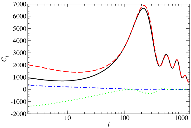
Figure 4.1: A decomposition of the best fit spectra (solid line) which has $\Delta=0$. The adiabatic (dashes), entropy (dash-dot) and correlation (dots) contributions are also plotted.

In the figure the adiabatic $([C_{l}]_{\rm ad})$, entropy ($B^{2}[C_{l}]_{\rm iso}$) and correlated $(2B\cos\Delta[C_{l}]_{\rm corr})$ components are shown. As can be seen, the effect of adding a positively correlated component is to reduce the height of the low-$l$ plateau relative to the acoustic peaks [47]. This is in contrast to the uncorrelated case where the addition of entropy perturbations reduces the peak height relative to the plateau.

We found a near-degeneracy between $B$ and $n$ when $\Delta=0$: the effect of adding maximally correlated isocurvature perturbations mimics an increase in the primordial slope. This makes clear the importance of varying $n$ when studying correlated isocurvature perturbations: a lower $n$ allows a larger $B$ to be consistent with the CMB data.

In Fig. 2 we plot a series of two-dimensional likelihood functions; all the other parameters have been marginalized in turn. The contour lines of the cosmological parameters $\omega_{b}$ and $\omega_{c}$ are almost parallel to $B$ for $B<1$. This means that the isocurvature perturbations do not alter significantly the best estimates for these cosmological parameters. On the other hand, increasing $B$ moves the region of confidence for $\Omega_{\Lambda}$ and of $n$ toward smaller values.

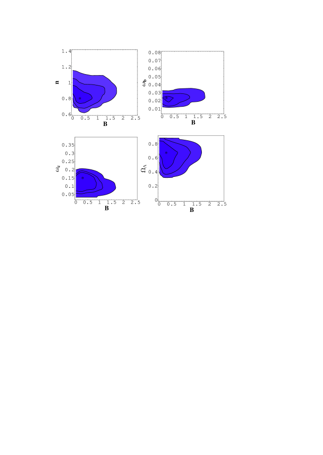
Figure 4.2: Two-dimensional likelihood contour plots. The contours enclose 40%, 86% and 99% of the likelihood and the stars mark the peaks. See text for explanation.

In Fig. 3 we plot the one-dimensional likelihood functions obtained by marginalizing all the remaining parameters. Panel a shows that the contribution of isocurvature perturbations can be as large as the adiabatic perturbations, or even larger: we find that $B<1.5$ to 95% c.l.. In contrast, if the isocurvature perturbations are uncorrelated, their fraction cannot exceed 70% ($B<0.7$) to the same c.l.. It is intriguing to observe that the likelihood of $B$ peaks around 0.3: that is, a non-zero contribution of isocurvature perturbations is more likely than a vanishing contribution. In the same panel we show as a long dashed line the likelihood assuming experimental errors reduced to one third, a precision within reach of the forthcoming satellite experiments: the curve shows that this level of precision would allow the detection of a finite isocurvature contribution. Equally interesting, in panel b we see that the likelihood of the correlation ${\rm cos}\Delta$ peaks near unity (maximal correlation), but has a not negligible probability everywhere in its domain. The likelihood functions for $n$ and $\Omega_{\Lambda}$ move toward smaller values, as anticipated, while the CDM and the baryon density estimates remain largely unaffected. The average values are

$$\begin{array}[]{l}n=0.87\pm 0.1,\quad\omega_{b}=0.023\pm 0.005,\\ \omega_{c}=0.12\pm 0.04,\quad\Omega_{\Lambda}=0.63\pm 0.13.\end{array}$$

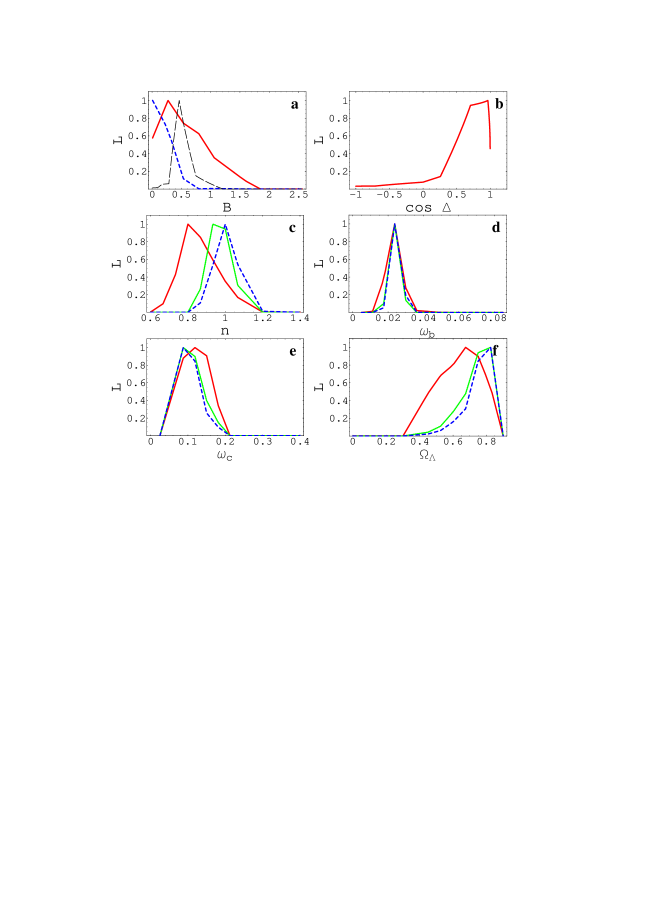
Figure 4.3: One-dimensional likelihood functions in arbitrary units. Green (light) solid lines for the purely adiabatic models ( $B=0$); blue short-dashed lines for uncorrelated fluctuations ($\cos\Delta=0$); red (dark) solid lines for correlated fluctuations. See text for further explanation.

4.4 Conclusions

By contrast, Enqvist et al [49] found that a large uncorrelated isocurvature contribution is only consistent with blue tilted slopes. The reason for this difference is that correlations can cause the acoustic peak height to increase relative to the Sachs Wolfe plateau (see Fig. 1) unlike the case of independent perturbations where the relative height always decreases. Trotta et al [79] found that the CMB data was not consistent with a significant CDM isocurvature contribution because they restricted the primordial slope, $n$, to be unity. As can be seen from Fig. 2 our $n=1$ likelihood contours also indicate a very low isocurvature contribution. But when $n$ is allowed to be less than one the isocurvature contribution can be even larger than the adiabatic contribution.

As can be seen from Figs. 2 and 3 our estimates of $\omega_{b}$ and $\omega_{c}$ are virtually unaffected by the addition of correlated CDM isocurvature perturbations. Thus, in our model, the nature of the isocurvature component can be investigated almost independently of the composition of the matter component.

The main conclusion of this Chapter is that Boomerang and Maxima are consistent with a large correlated CDM isocurvature perturbation contribution when the spectral slopes are tilted to the red ($n<1$). The higher precision of future satellite data has the potential to detect the isocurvature contribution, if any, thereby showing that inflation was not a single-field process.

Chapter 5 Non-adiabatic perturbations from brane world effects

5.1 Introduction

According to string and M-theory, gravity is a higher-dimensional theory, reducing to Einstein’s four-dimensional theory of general relativity at low enough energies. In the brane-world scenario, the standard model matter fields are confined to a 3-brane in $1+3+d$ dimensions, while the gravitational field can propagate in the bulk, i.e., also in the $d$ extra dimensions, being localized at the brane at low energies. Recent developments show that the $d$ extra space dimensions need not be small, or even compact, thus allowing the intriguing possibility that corrections could occur even at TeV scales.

These exciting theoretical developments may offer a promising route towards a quantum gravity theory. However, as well as theoretical elegance, they must also pass the increasingly stringent tests provided by cosmological observations. Primarily, this involves developing higher-dimensional perturbation theory and then applying it to analyze the generation and evolution of density and tensor perturbations on the brane, leading to a prediction of the CMB anisotropies and galaxy distribution.

This is an ambitious and difficult programme, but initial steps have already been taken, at least in the case of a particular class of models that generalize the Randall-Sundrum models [20]. Large-scale adiabatic density perturbations from inflation on the brane have been computed [82] (see also [83]), using the conservation of the curvature perturbation on uniform-density hypersurfaces. This conservation follows from adiabaticity and the conservation of energy-momentum on the brane, and is independent of the form of the field equations [27]. In [82], the backreaction effect of metric fluctuations in the fifth dimension was neglected. In the general case, i.e., incorporating also the fluctuations in the nonlocal quantities that carry the bulk influence onto the brane, it has been shown that large-scale density perturbations contain a closed system on the brane—and thus can in principle be evaluated purely from initial conditions on the brane, without knowledge of bulk dynamics [84]. Note that not all large-scale scalar perturbations can be computed intrinsically – the relation between the metric potentials $A$ and $\Psi$ is mediated by anisotropic stress imprinted on the brane by the bulk Weyl tensor and this stress cannot be evaluated without solving the bulk equations [85]. In this Chapter, we solve the closed system described in [84] to find the evolution of large-scale density perturbations on the brane. We show that extra-dimensional effects introduce a non-adiabatic mode on the brane.

A general perturbation formalism has been developed [86, 87], encompassing equations on the brane and in the bulk, and in principle able to describe all scales. However, the general equations are extremely complicated, in particular since the mode equations are partial differential equations. A first application of the equations has been made to large-scale tensor perturbations from inflation on the brane [88]. Unlike the scalar case, large-scale tensor perturbations cannot be evaluated without the bulk perturbation equations.

We develop the outline argument presented first in [84], and analyze large-scale density perturbations and their evolution, from after Hubble-crossing in inflation through the radiation era. This provides part of the information needed for predicting the large-angle scalar anisotropies generated in CMB temperature, and seeing how the bulk effects modify general relativistic predictions. However, the Sachs-Wolfe (SW) effect cannot be computed without knowledge of the Weyl anisotropic stress [85]. It is possible to estimate the SW effect by making assumptions about the Weyl anisotropic stress [89], but a complete solution requires solving the full 5D perturbation problem.

We show that in general, the perturbation $\Phi$ (a covariant analog of the Bardeen metric perturbation) is no longer constant during high-energy inflation, but grows. However, $\Phi$ is constant during the radiation era, as in general relativity, except at most in the early radiation era, if the energy density is still high relative to the brane tension.

5.2 Brane dynamics

We follow the 1+3 covariant approach and notation of [84] which is different from (but ultimately equivalent to) the metric-based approach to perturbations described in Chapter 2. The 5-dimensional (bulk) field equations are

$$\widetilde{G}_{AB}=\widetilde{\kappa}^{2}\left[-\widetilde{\Lambda}\widetilde{g}_{AB}+\delta(\chi)\left\{-\lambda g_{AB}+T_{AB}\right\}\right]\,,$$ (5.1)

where tildes denote the bulk generalization of standard general relativity quantities, and $\widetilde{\kappa}^{2}=8\pi/\widetilde{M}_{\rm p}^{3}$, where $\widetilde{M}_{\rm p}$ is the fundamental 5-dimensional Planck mass, which is typically much less than the effective Planck mass on the brane, $M_{\rm p}=1.2\times 10^{19}$ GeV. The brane is given by $\chi=0$, so that a natural choice of coordinates is $x^{A}=(x^{\mu},\chi)$, where $x^{\mu}=(t,x^{i})$ are spacetime coordinates on the brane and the brane a moving hypersurface. The brane tension is $\lambda$, and $g_{AB}=\widetilde{g}_{AB}-n_{A}n_{B}$ is the induced metric on the brane, with $n_{A}$ the spacelike unit normal to the brane. Standard-model matter fields confined to the brane make up the brane energy-momentum tensor $T_{AB}$ (with $T_{AB}n^{B}=0$). The bulk cosmological constant $\widetilde{\Lambda}$ is negative, and is the only 5-dimensional stress energy. (See [90] for the modification of this approach in the case where there is also a scalar field in the bulk.)

The most general background bulk with homogeneous and isotropic induced metric on the brane is the 5-dimensional Schwarzschild-anti-de Sitter metric [91], with the black hole mass leading to an effective radiation-like correction to the Friedmann equation on the brane [92].

The field equations induced on the brane are derived via an elegant geometric approach in [93], leading to new terms that carry bulk effects onto the brane:

$$G_{\mu\nu}=-\Lambda g_{\mu\nu}+\kappa^{2}T_{\mu\nu}+\widetilde{\kappa}^{4}S_{\mu\nu}-{\cal E}_{\mu\nu}\,,$$ (5.2)

where $\kappa^{2}=8\pi/M_{\rm p}^{2}$. The various energy scales are related to each other via

$$\lambda=6{\kappa^{2}\over\widetilde{\kappa}^{4}}\,,~{}~{}\Lambda={\textstyle{1\over 2}}\widetilde{\kappa}^{2}\left(\widetilde{\Lambda}+{\textstyle{1\over 6}}\widetilde{\kappa}^{2}\lambda^{2}\right)\,,$$ (5.3)

and the high-energy regime is $\rho\stackrel{{\scriptstyle>}}{{\sim}}\lambda$. Bulk corrections to the Einstein equations on the brane are of two forms: firstly, the matter fields contribute local quadratic energy-momentum corrections via the tensor $S_{\mu\nu}$, and secondly, there are nonlocal effects from the free gravitational field in the bulk, transmitted via the projection ${\cal E}_{\mu\nu}$ of the bulk Weyl tensor. The matter corrections are given by

$$S_{\mu\nu} = {\textstyle{1\over 12}}T_{\alpha}{}^{\alpha}T_{\mu\nu}-{\textstyle{1\over 4}}T_{\mu\alpha}T^{\alpha}{}_{\nu}$$ (5.4)

$$~{}~{}{}+{\textstyle{1\over 24}}g_{\mu\nu}\left[3T_{\alpha\beta}T^{\alpha\beta}-\left(T_{\alpha}{}^{\alpha}\right)^{2}\right]\,.$$

The projection of the bulk Weyl tensor is

$${\cal E}_{AB}=\widetilde{C}_{ACBD}n^{C}n^{D}\,,$$ (5.5)

which is symmetric and traceless and without components orthogonal to the brane, so that ${\cal E}_{AB}n^{B}=0$ and ${\cal E}_{AB}\to{\cal E}_{\mu\nu}g_{A}{}^{\mu}g_{B}{}^{\nu}$ as $\chi\to 0$.

The Weyl tensor $\widetilde{C}_{ABCD}$ represents the free, nonlocal gravitational field in the bulk, i.e., the part of the field that is not directly determined at each point by the energy-momentum tensor at that point. The local part of the bulk gravitational field is the Einstein tensor $\widetilde{G}_{AB}$, which is determined locally via the bulk field equations (5.1). Thus ${\cal E}_{\mu\nu}$ transmits nonlocal gravitational degrees of freedom from the bulk to the brane, including tidal (or Coulomb), gravito-magnetic and transverse traceless (gravitational wave) effects [84].

If $u^{\mu}$ is the 4-velocity comoving with matter (which we assume is a perfect fluid or minimally-coupled scalar field), we can decompose the nonlocal term as

$${\cal E}_{\mu\nu}={-6\over\kappa^{2}\lambda}\left[{\cal U}\left(u_{\mu}u_{\nu}+{\textstyle{1\over 3}}h_{\mu\nu}\right)+{\cal P}_{\mu\nu}+{\cal Q}_{\mu}u_{\nu}+{\cal Q}_{\nu}u_{\mu}\right]\,,$$ (5.6)

where $h_{\mu\nu}=g_{\mu\nu}+u_{\mu}u_{\nu}$ projects into the comoving rest-space. Here

$${\cal U}=-{\textstyle{1\over 6}}\kappa^{2}\lambda\,{\cal E}_{\mu\nu}u^{\mu}u^{\nu}$$

is an effective nonlocal energy density on the brane (which need not be positive), arising from the free gravitational field in the bulk. It carries Coulomb-type effects from the bulk onto the brane. There is an effective nonlocal anisotropic stress

$${\cal P}_{\mu\nu}=-{\textstyle{1\over 6}}\kappa^{2}\lambda\left[h_{\mu}{}^{\alpha}h_{\nu}{}^{\beta}-{\textstyle{1\over 3}}h^{\alpha\beta}h_{\mu\nu}\right]{\cal E}_{\alpha\beta}$$

on the brane, which carries Coulomb, gravito-magnetic and gravitational wave effects of the free gravitational field in the bulk. The effective nonlocal energy flux on the brane,

$${\cal Q}_{\mu}={\textstyle{1\over 6}}\kappa^{2}\lambda\,h_{\mu}{}^{\alpha}{\cal E}_{\alpha\beta}u^{\beta}\,,$$

carries Coulomb and gravito-magnetic effects from the free gravitational field in the bulk. (Note that there is no energy flux in the bulk, and thus no transfer of energy between bulk and brane; this situation changes if bulk scalar fields are present [87, 90].)

5.3 Local and nonlocal conservation equations

The local and nonlocal bulk modifications may be consolidated into an effective total energy-momentum tensor:

$$G_{\mu\nu}=-\Lambda g_{\mu\nu}+\kappa^{2}T^{\rm tot}_{\mu\nu}\,,$$ (5.7)

where

$$T^{\rm tot}_{\mu\nu}=T_{\mu\nu}+{6\over\lambda}S_{\mu\nu}-{1\over\kappa^{2}}{\cal E}_{\mu\nu}\,.$$ (5.8)

The effective total energy density, pressure, anisotropic stress and energy flux are

$$\rho^{\rm tot} = \rho\left(1+{\rho\over 2\lambda}\right)+{6{\cal U}\over\kappa^{4}\lambda}\,,$$ (5.9)

$$p^{\rm tot} = p+{\rho\over 2\lambda}(\rho+2p)+{2{\cal U}\over\kappa^{4}\lambda}\,,$$ (5.10)

$$\pi^{\rm tot}_{\mu\nu} = {6\over\kappa^{4}\lambda}{\cal P}_{\mu\nu}\,,$$ (5.11)

$$q^{\rm tot}_{\mu} = {6\over\kappa^{4}\lambda}{\cal Q}_{\mu}\,.$$ (5.12)

The brane energy-momentum tensor separately satisfies the conservation equations, $\nabla^{\nu}T_{\mu\nu}=0$, giving

$$\dot{\rho}+\Theta(\rho+p)=0\,,$$ (5.13)

$$\mbox{D}_{\mu}p+(\rho+p)A_{\mu}=0\,,$$ (5.14)

where a dot denotes $u^{\nu}\nabla_{\nu}$, $\Theta=\mbox{D}^{\mu}u_{\mu}$ is the volume expansion rate of the $u^{\mu}$ congruence, $A_{\mu}=\dot{u}_{\mu}$ is its 4-acceleration, and $\mbox{D}_{\mu}$ is the projected covariant spatial derivative. The Bianchi identities on the brane imply that the projected Weyl tensor obeys the constraint

$$\nabla^{\mu}{\cal E}_{\mu\nu}={6\kappa^{2}\over\lambda}\nabla^{\mu}S_{\mu\nu}\,.$$ (5.15)

This shows how nonlocal bulk effects are sourced by local bulk effects, which include spatial gradients and time derivatives: evolution and inhomogeneity in the matter fields can generate nonlocal gravitational effects in the bulk, which backreact on the brane. The brane energy-momentum tensor and the consolidated effective energy-momentum tensor are both conserved separately. Conservation of $T^{\rm tot}_{\mu\nu}$ gives, upon using Eqs. (5.9)–(5.14), propagation equations for the nonlocal energy density ${\cal U}$ and energy flux ${\cal Q}_{\mu}$. In linearized form, these are

$$\dot{\cal U}+{\textstyle{4\over 3}}\Theta{\cal U}+\mbox{D}^{\mu}{\cal Q}_{\mu}=0\,,$$ (5.16)

$$\dot{\cal Q}_{\mu}+4H{\cal Q}_{\mu}+{\textstyle{1\over 3}}\mbox{D}_{\mu}{\cal U}+{\textstyle{4\over 3}}{\cal U}A_{\mu}$$

$$~{}~{}~{}{}+\mbox{D}^{\nu}{\cal P}_{\mu\nu}=-{\textstyle{1\over 6}}\kappa^{4}(\rho+p)\mbox{D}_{\mu}\rho\,,$$ (5.17)

where $H=\dot{a}/a$ ($={1\over 3}\Theta$) is the Hubble rate in the background. The nonlocal tensor mode, which is the part of ${\cal P}_{\mu\nu}$ that satisfies $\mbox{D}^{\nu}{\cal P}_{\mu\nu}=0\neq{\cal P}_{\mu\nu}$, does not enter the nonlocal conservation equations. Furthermore, there is no evolution equation at all for ${\cal P}_{\mu\nu}$, reflecting the fact that in general the equations do not close on the brane, and one needs bulk equations to determine brane dynamics. There are bulk degrees of freedom whose impact on the brane cannot be predicted by brane observers, for example, incoming gravitational radiation from the bulk. The evolution of the nonlocal energy density and flux, which carry scalar and vector modes of the bulk gravitational field, is determined on the brane, while the evolution of the nonlocal anisotropic stress, which carries scalar, vector and tensor modes of the bulk field, is not.

The generalized Raychaudhuri equation on the brane in linearized form is

$$\dot{\Theta}+{\textstyle{1\over 3}}\Theta^{2}-{\rm D}^{\mu}A_{\mu}+{\textstyle{1\over 2}}\kappa^{2}(\rho+3p)-\Lambda$$

$$~{}~{}{}=-{\textstyle{1\over 2}}\kappa^{2}(2\rho+3p){\rho\over\lambda}-{6{\cal U}\over\kappa^{2}\lambda}\,,$$ (5.18)

where the general relativistic case is recovered when the right-hand side is set to zero. In the background, this gives

$$\dot{H} = -H^{2}-{\kappa^{2}\over 6}\left[\rho+3p+{\rho\over 2\lambda}(2\rho+3p)\right]$$ (5.19)

$$~{}~{}{}+{1\over 3}\Lambda-{2\over\kappa^{2}\lambda}{\cal U}_{o}\left({a_{o}\over a}\right)^{4}\,,$$

where the solution for ${\cal U}$ follows from Eq. (5.16), $a_{o}$ is the initial scale factor and ${\cal U}_{o}={\cal U}(a_{o})$. The first integral of this equation is the generalized Friedmann equation on the brane:

$$H^{2}={\kappa^{2}\over 3}\rho\left(1+{\rho\over 2\lambda}\right)+{1\over 3}\Lambda-{K\over a^{2}}+{2\over\kappa^{2}\lambda}{\cal U}_{o}\left({a_{o}\over a}\right)^{4}\,,$$ (5.20)

where $K=0,\pm 1$. Local bulk effects modify the background dynamics. In particular, inflation at high energies ($\rho\stackrel{{\scriptstyle>}}{{\sim}}\lambda$) proceeds at a higher rate than the corresponding rate in general relativity. This introduces important changes to the dynamics of the early universe [82, 83, 94], and accounts for an increase in the amplitude of scalar and tensor fluctuations at Hubble-crossing [82, 88].

Using Eqs. 5.20 and 5.19 the condition for inflation becomes [82]

$$w<-{1\over 3}\left({2\rho+\lambda\over\rho+\lambda}\right)\,,$$ (5.21)

where $w=p/\rho$. As $\rho/\lambda\to\infty$, we have $w<-{2\over 3}$, while the general relativity condition $w<-{1\over 3}$ is recovered as $\rho/\lambda\to 0$.

If ${\cal U}_{o}=0$, i.e., if the background bulk is conformally flat, then Eqs. (5.9) and (5.10) show that the effective equation of state index for the total energy-momentum tensor is

$$w^{\rm tot}\equiv{p^{\rm tot}\over\rho^{\rm tot}}={w+(1+2w)\rho/2\lambda\over 1+\rho/2\lambda}\approx 1+2w\,,$$ (5.22)

where the last equality holds at very high energies ($\rho\gg\lambda$). Thus for slow-roll inflation, $w^{\rm tot}$ and $w$ are both close to $-1$. The high-energy inflation condition $w<-{2\over 3}$ is $w^{\rm tot}<-{1\over 3}$. During high-energy reheating with $w\approx 0$ on average, we have $w^{\rm tot}\approx 1$, so that the effective equation of state is stiff, while high-energy radiation-domination ($w={1\over 3}$) has $w^{\rm tot}\approx{5\over 3}$, i.e., an ultra-stiff effective equation of state. The effective sound speed at very high energies is also altered:

$$(c_{\rm s}^{2})^{\rm tot}\equiv{\dot{p}^{\rm tot}\over\dot{\rho}^{\rm tot}}\approx c_{\rm s}^{2}+w+1\,,$$ (5.23)

where $c_{\rm s}^{2}=\dot{p}/\dot{\rho}$.

5.4 Scalar perturbations on the brane

When the vorticity of the fluid vanishes, scalar perturbations are covariantly (as well as gauge-invariantly and locally) characterized as the case when all perturbed quantities are expressible as spatial gradients of scalars. In particular, the nonlocal perturbed bulk effects are described by $\mbox{D}_{\mu}{\cal U}$ and [84]

$${\cal Q}_{\mu}=\mbox{D}_{\mu}{\cal Q}\,,~{}~{}{\cal P}_{\mu\nu}=\left[h_{\mu}{}^{\alpha}h_{\nu}{}^{\beta}-{\textstyle{1\over 3}}h^{\alpha\beta}h_{\mu\nu}\right]\mbox{D}_{\alpha}\mbox{D}_{\beta}{\cal P}\,.$$ (5.24)

Note that the nonlocal traceless mode has spatial divergence [84]:

$$\mbox{D}^{\nu}{\cal P}_{\mu\nu}={\textstyle{2\over 3}}\mbox{D}^{2}(\mbox{D}_{\mu}{\cal P})\,.$$

The bulk gravitational field affects scalar perturbations via scalar Coulomb modes, given by the spatial gradients of the ‘potentials’ ${\cal U}$, ${\cal Q}$ and ${\cal P}$.

For adiabatic matter perturbations the 4-acceleration is

$$A_{\mu}=-{c_{\rm s}^{2}\over\rho(1+w)}\,\mbox{D}_{\mu}\rho\,.$$ (5.25)

The gradients

$$\Delta_{\mu}={a\over\rho}\mbox{D}_{\mu}\rho\,,~{}~{}Z_{\mu}=a\mbox{D}_{\mu}\Theta\,,$$ (5.26)

describe inhomogeneities in the matter and expansion [95], and the dimensionless gradients describing inhomogeneity in the nonlocal quantities are [84]

$$U_{\mu}={a\over\rho}\mbox{D}_{\mu}{\cal U}\,,~{}Q_{\mu}={1\over\rho}\mbox{D}_{\mu}{\cal Q}\,,~{}P_{\mu}={1\over a\rho}\mbox{D}_{\mu}{\cal P}\,.$$ (5.27)

The spatial gradient of the conservation equations (5.13), (5.16) and (5.17), and the generalized Raychaudhuri equation (5.18), leads to a system of equations for these gradient quantities [84]. The gradients define scalars via their comoving divergences:

$$F\equiv a\mbox{D}^{\mu}F_{\mu}\,,~{}\mbox{ with }~{}F=\Delta,Z,U,Q,P\,,$$ (5.28)

where $\Delta$ is a covariant analog of the Bardeen density perturbation $\epsilon_{\rm m}$ (see Eq. 2.10). Then the system of equations governing scalar perturbations on the brane follows from the gradient system given in [84] as

$$\dot{\Delta}=3wH\Delta-(1+w)Z\,,$$ (5.29)

$$\dot{Z}=-2HZ-\left({c_{\rm s}^{2}\over 1+w}\right)\mbox{D}^{2}\Delta-\left({6\rho\over\kappa^{2}\lambda}\right)U$$

$$~{}~{}{}-{\textstyle{1\over 2}}\kappa^{2}\rho\left[1+(4+3w){\rho\over\lambda}-\left({2c_{\rm s}^{2}\over 1+w}\right){6{\cal U}\over\kappa^{4}\lambda\rho}\right]\Delta\,,$$ (5.30)

$$\dot{U}=(3w-1)HU-\left({4c_{\rm s}^{2}\over 1+w}\right)\left({{\cal U}\over\rho}\right)H\Delta$$

$$~{}~{}{}-\left({4{\cal U}\over 3\rho}\right)Z-a\mbox{D}^{2}Q\,,$$ (5.31)

$$\dot{Q}=(1-3w)HQ-{1\over 3a}U-{\textstyle{2\over 3}}a\mbox{D}^{2}P$$

$$~{}~{}{}+{1\over 6a}\left[\left({8c_{\rm s}^{2}\over 1+w}\right){{\cal U}\over\rho}-\kappa^{4}\rho(1+w)\right]\Delta\,.$$ (5.32)

In general relativity, only the first two equations apply, with $\lambda^{-1}$ set to zero in Eq. (5.30). In this case we can decouple the density perturbations via a second-order equation for $\Delta$, whose independent solutions are adiabatic growing and decaying modes. Local bulk effects modify the background dynamics, while nonlocal bulk effects introduce new fluctuations. This leads to fundamental changes to the simple general relativity picture. There is no equation for $\dot{P}$, so that in general, scalar perturbations on the brane cannot be predicted by brane observers without additional information from the unobservable bulk. Thus in general, one must solve also the scalar perturbations in the bulk in order to determine the perturbation evolution on the brane.

However, there is a crucially important exception to this, arising from the fact that $P$ only occurs in Eqs. (5.29)–(5.32) via the Laplacian term $\mbox{D}^{2}P$. We can use the shear propagation equation on the brane [84] to provide an order-of-magnitude comparison of $P$ with $\Delta$:

$$\dot{\sigma}_{\mu\nu}+2H\sigma_{\mu\nu}+E_{\mu\nu}+\mbox{D}_{\langle\mu}A_{\nu\rangle}={3\over\kappa^{2}\lambda}{\cal P}_{\mu\nu}\,,$$

where $E_{\mu\nu}$ is the electric Weyl tensor on the brane. This equation, together with Eqs. (5.24) and (5.25) shows that

$${1\over\kappa^{2}\lambda}|\mbox{D}^{2}{\cal P}|\sim{1\over\rho}|\mbox{D}^{2}\rho|\,,$$

and then Eqs. (5.26)–(5.28) imply

$$|P|\sim{\kappa^{2}\lambda\over a^{2}\rho}|\Delta|\,.$$

Then

$$|a\mbox{D}^{2}P|\sim{k^{2}\over a^{2}H^{2}}\,{\kappa^{4}\rho\over a}|\Delta|\,,$$

on using the high-energy Friedmann equation ($H^{2}\sim\kappa^{2}\rho^{2}/\lambda$). Thus, for $k\ll aH$, i.e. on large scales, well beyond the Hubble horizon, we can neglect the $\mbox{D}^{2}P$ term in Eq. (5.32) relative to the $\Delta$ term. Thus on large scales, the system closes on the brane, and brane observers can predict scalar perturbations from initial conditions intrinsic to the brane, without the need to solve the bulk perturbation equations. Note that the $\mbox{D}^{2}Q$ term in Eq. (5.31) may also be neglected relative to the $U$ term. This follows from the shear constraint equation [84]

$$\mbox{D}^{\nu}\sigma_{\mu\nu}-{\textstyle{2\over 3}}\mbox{D}_{\mu}\Theta=-{6\over\kappa^{2}\lambda}{\cal Q}_{\mu}\,,$$

which gives, on taking the divergence,

$$|Q|\sim{\kappa^{2}\lambda\over a\rho}|Z|\sim{1\over aH}|U|\,,$$

where the last relation follows from Eq. (5.30). Thus

$$|aD^{2}Q|\sim\frac{k^{2}}{a^{2}H^{2}}(H|{U}|)$$

and so we may neglect the $D^{2}Q$ term in Eq. 5.31 relative to the $U$ term. The system Eqs. (5.29)–(5.32) then reduces to 3 coupled equations in $\Delta$, $Z$ and $U$, plus a decoupled equation for $Q$, which determines $Q$ once the other 3 quantities are solved for. Thus there are in general 3 modes of large-scale density perturbations: a non-adiabatic mode is introduced by bulk effects. This mode is carried by fluctuations $U$ in the nonlocal energy density ${\cal U}$, which are present even if ${\cal U}$ vanishes in the background. The fluctuations $Q$ and $P$ in the nonlocal energy flux and anisotropic stress do not affect the density perturbations on very large scales.

In qualitative terms, we can interpret these general results as follows. Bulk effects lead to an effective total energy-momentum tensor that is non-adiabatic. From Eqs. (5.9) and (5.10), we find a measure of the total effective non-adiabatic pressure perturbation, which is the covariant analog of $\delta p^{\rm tot}-(c_{\rm s}^{2})^{\rm tot}\delta\rho^{\rm tot}$:

$$a\mbox{D}_{\mu}p^{\rm tot}-(c_{\rm s}^{2})^{\rm tot}a\mbox{D}_{\mu}\rho^{\rm tot}={6H\rho\over\kappa^{4}\dot{\rho}^{\rm tot}\lambda}\left(1+{\rho\over\lambda}\right)\times$$

$$~{}{}\times\left[{1\over 3}-c_{\rm s}^{2}-{\rho+p\over\rho+\lambda}\right]\left\{4{\cal U}\,\Delta_{\mu}-3(\rho+p)U_{\mu}\right\}\,.$$ (5.33)

In addition, Eqs. (5.11) and (5.12) show that non-adiabatic stresses and fluxes are also present, due to nonlocal bulk effects. From this viewpoint, it is not surprising that non-adiabatic modes arise in the density perturbations. An analysis of the non-adiabatic large scale mode in terms of the curvature perturbation is given in [85].

Note that an alternative interpretation is also possible. We can regard the nonlocal bulk effects as constituting a radiative “Weyl” fluid, with energy-momentum tensor $-\kappa^{-2}{\cal E}_{\mu\nu}$. This Weyl fluid has non-adiabatic stresses ${\cal P}_{\mu\nu}$, and is in motion relative to the matter fluid, with relative velocity parallel to ${\cal Q}_{\mu}$. Although the matter fluid obeys energy-momentum conservation, the Weyl fluid does not; the momentum balance equation (5.17) shows that density inhomogeneity in the matter fluid sources a momentum transfer to the Weyl fluid.

Whatever intuitive interpretation we adopt, the concrete result is that large-scale density perturbations on the brane may be determined without knowledge of the bulk, and acquire a non-adiabatic mode due to effects from the free gravitational field in the bulk.

5.5 Large-scale density perturbations

We rewrite the coupled system for large-scale perturbations by introducing two useful new quantities. We define, following [95],

$$\Phi=\kappa^{2}\rho a^{2}\Delta\,,$$ (5.34)

which is a covariant analog of the Bardeen metric potential $\Phi_{H}$ (see Chapter 2), and the covariant local curvature perturbation

$$C=a\mbox{D}^{\mu}C_{\mu}\,,~{}C_{\mu}=a^{3}\mbox{D}_{\mu}{R^{\perp}}\,,$$ (5.35)

where ${R^{\perp}}$ is the Ricci curvature of the surfaces orthogonal to $u^{\mu}$. (Note that these surfaces are in general shearing, and non-uniform in $\rho$, $\Theta$, ${\cal U}$ and ${R^{\perp}}$.)

Then the coupled system for density perturbations, Eqs. (5.29)–(5.31), can be rewritten on large scales as

$$\dot{\Phi} = -H\left[1+{(1+w)\kappa^{2}\rho\over 2H^{2}}\left(1+{\rho\over\lambda}\right)\right]\Phi$$ (5.36)

$$~{}~{}{}+\left[{(1+w)\kappa^{2}\rho\over 4H}\right]C-\left[{3(1+w)a^{2}\rho^{2}\over\lambda H}\right]U\,,$$

$$\dot{C} = -\left[{72c_{\rm s}^{2}H{\cal U}\over(1+w)\lambda\kappa^{2}\rho}\right]\Phi\,,$$ (5.37)

$$\dot{U} = H\left[3w-1-{4{\cal U}\over\kappa^{2}\lambda H^{2}}\right]U+\left({{\cal U}\over 3a^{2}H\rho}\right)C$$ (5.38)

$$~{}~{}{}-{2{\cal U}\over 3a^{2}H\rho}\left[1+{\rho\over\lambda}+{6c_{\rm s}^{2}H^{2}\over(1+w)\kappa^{2}\rho}\right]\Phi\,.$$

The general relativistic case is recovered when we set $\lambda^{-1}$, ${\cal U}$ and $U$ to zero; in this case, Eq. (5.38) falls away, and Eq. (5.37) reduces to

$$C=C_{o}\,,~{}~{}\dot{C}_{o}=0\,,$$ (5.39)

which expresses conservation of the covariant curvature perturbation along each fundamental world-line. The value of $C_{o}$ will in general vary from world-line to word-line, so that its conservation is local, and is not an indicator of purely adiabatic perturbations. (In general relativity, $\dot{C}=0$ on large scales for a flat background even when there are non-adiabatic perturbations [95].) Bulk effects destroy the local conservation of $C$ in general, by Eq. (5.37).

However, there is an important special case when local conservation is regained: when the nonlocal energy density ${\cal U}$ vanishes in the background. This does not mean that fluctuations in the nonlocal energy density are zero, i.e., we still have $U\neq 0$ in general. It can be argued that vanishing ${\cal U}$ in the background is more natural, if one believes that the bulk background should be conformally flat, and thus strictly anti-de Sitter. (Quantum effects may nucleate a black hole in the bulk [96], in which case the Schwarzschild-anti de Sitter bulk, with ${\cal U}_{o}$ proportional to the black hole mass, would be a natural background.) From now on, we will assume a conformally flat background bulk and a spatially flat brane background; thus ${\cal U}_{o}=0=K$ in the background generalized Friedmann equation (5.20). Equation (5.4) shows that the non-adiabatic total pressure perturbation is then proportional to $(\rho/\lambda)U$, which will be enhanced at high energies and suppressed at low energies.

When ${\cal U}=0$ in the background, Eq. (5.39) holds, and Eq. (5.38) gives

$$U=U_{o}f\,,~{}\dot{U}_{o}=0\,,~{}f=\exp\int_{a_{o}}^{a}(3w-1)\,d\ln a\,.$$ (5.40)

This shows that $U$ rapidly redshifts away during inflation, so that non-adiabatic effects from nonlocal bulk influence are small. By contrast, the modifications to the background dynamics from local bulk effects are strong during inflation at high energy.

The key equation (5.36) becomes

$${d\Phi\over dN}+\left[1+{(1+w)\kappa^{2}\rho\over 2H^{2}}\left(1+{\rho\over\lambda}\right)\right]\Phi=$$

$$~{}{}\left[{(1+w)\kappa^{2}\rho\over 4H^{2}}\right]C_{o}-\left[{3(1+w)a_{o}^{2}\rho^{2}\over\lambda H^{2}}\right]e^{2N}fU_{o}\,,$$ (5.41)

where $N=\ln(a/a_{o})$ is the number of e-folds. We have thus reduced the coupled system to one simple inhomogeneous linear equation, which may be integrated along the fundamental world-lines. Along each world-line, the constancy of $C_{o}$ and $U_{o}$ allows us to track the change in $\Phi$ as $w$ changes, from inflationary behavior through to radiation- and matter-domination.

We can perform a qualitative analysis of the evolution of $\Phi$ as follows. Substituting $H^{2}$ from the generalized Friedman Eq. (5.20) into Eq. (5.41) and setting ${\cal U}_{0}$, $K$ and $\Lambda$ to zero gives

$$\begin{array}[]{l}{\frac{d\Phi}{dN}}+\left(1+\frac{3}{2}\,\left(1+w\right)\left(1+{\frac{\rho}{\lambda}}\right)\left(1+\frac{1}{2}\,{\frac{\rho}{\lambda}}\right)^{-1}\right)\Phi\\ =\frac{3}{4}\,\left(1+w\right)C_{{0}}\left(1+\frac{1}{2}\,{\frac{\rho}{\lambda}}\right)^{-1}\\ -9\,\left(1+w\right){{a_{0}}}^{2}\rho\,{e^{N\left(1+3\,w\right)}}U_{{0}}{\lambda}^{-1}{\kappa}^{-2}\left(1+\frac{1}{2}\,{\frac{\rho}{\lambda}}\right)^{-1}\end{array}$$ (5.42)

For high-energy inflation $\rho\gg\lambda$ and so we can approximate Eq. (5.42) by

$${\frac{d\Phi}{dN}}+\left(4+3\,w\right)\Phi=\frac{3}{2}\,{\frac{\left(1+w\right)C_{{0}}\lambda}{\rho}}-18\,{\frac{\left(1+w\right){{a_{0}}}^{2}{e^{N\left(1+3\,w\right)}}U_{{0}}}{{\kappa}^{2}}}$$ (5.43)

As it is slow-roll inflation, we can assume $w$ and $\rho$ are constant when solving this equation. This gives

$$\Phi\approx\left(1+w\right)\left(\frac{3}{2}\,{\frac{\lambda\,C_{{0}}}{\left(4+3\,w\right)\rho}}-18\,{\frac{U_{{0}}{{a_{0}}}^{2}{e^{N\left(1+3\,w\right)}}}{\left(5+6\,w\right){\kappa}^{2}}}\right)+{e^{\left(-4-3\,w\right)N}}{C_{1}}$$ (5.44)

where $C_{1}$ is an integration constant. Using $w\approx-1$ and dropping the exponentially decaying terms this gives

$$\mbox{high-energy inflation:}~{}~{}~{}\Phi\approx{3\over 2}(1+w)C_{o}\,{\lambda\over\rho}\,.$$ (5.45)

For the general relativity limit we use $\lambda\gg\rho$ and then following the same procedure as for the high energy case we get

$$\Phi_{\rm gr}\approx{3\over 4}(1+w)C_{o}\,.$$ (5.46)

In general relativity, $\Phi$ remains constant on large scales during slow-roll inflation, independent of the form of the inflaton potential. In the brane-world, $\Phi$ is slowly increasing during high-energy slow-roll inflation, since $\Phi\sim\rho^{-1}$ and $\rho$ is slowly decreasing. This qualitative analysis is confirmed by the numerical integration of a simple phenomenological model shown in Fig. 1. We have modelled a smooth transition from inflation to radiation by $w={1\over 3}[(2-\alpha)\tanh(N-50)-(1-\alpha)]$, where $\alpha$ is a small positive parameter (chosen as $\alpha=0.1$ in the plot). For more realistic models, i.e., where $V(\varphi)$ is specified, the evolution of $\Phi$ may be more complicated than shown in Fig. 1. For $\rho_{o}/\lambda\gg 1$, Eq. (5.21) shows that inflation ends at $N=50-2\ln[(1-2\alpha)/3]\approx 47.4$, and at $N=50$ in general relativity. Only the lowest curve still has $\rho/\lambda\gg 1$ at the start of radiation-domination ($N$ greater than about 53), and one can see that $\Phi$ is still growing, as confirmed by Eq. (5.49).

During reheating, in periods when $w$ is approximately constant on average (for example, $w\approx 0$ for $V={1\over 2}m^{2}\varphi^{2}$), Eqs. (5.13) and (5.41) imply

high-energy $$w\approx$$ constant reheating:

$$~{}~{}~{}~{}~{}\Phi\approx{3(1+w)\over 2(7+6w)}{\lambda\over\rho_{0}}C_{o}\,e^{3(1+w)N}+\,{\rm const}\,.$$ (5.47)

Thus high-energy $w\approx$ constant reheating on the brane produces amplification of $\Phi$, unlike general relativity, where $\Phi$ remains constant on large scales during $w\approx$ constant reheating:

$$\Phi_{\rm gr}\approx{3(1+w)\over 2(5+3w)}C_{o}\,.$$ (5.48)

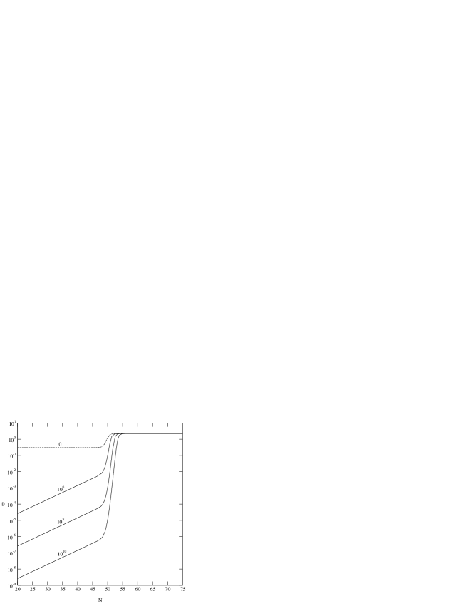
Figure 5.1: The evolution of $\Phi$ along a fundamental world-line for a mode that is well beyond the Hubble horizon at $N=0$, about 50 e-folds before inflation ends, and remains super-Hubble through the radiation era. Labels on the curves indicate the value of $\rho_{o}/\lambda$, so that the general relativistic solution is the dashed curve ($\rho_{o}/\lambda=0$).

In the radiation era, the energy density redshifts rapidly, so that $\rho$ quickly falls below the brane tension $\lambda$. If the energy density at the end of reheating is high enough, then at the start of radiation-domination we have $\rho\gg\lambda$, and we find that $\Phi$ is amplified during high-energy radiation domination:

$$\mbox{high-energy radiation:}~{}~{}~{}\Phi\approx{2\over 9}{\lambda\over\rho_{0}}\,C_{o}e^{4N}+\,{\rm const}\,.$$ (5.49)

At low energies on the brane, or in general relativity, we find that $\Phi$ is constant:

$$\mbox{low-energy radiation:}~{}~{}~{}\Phi\approx\Phi_{\rm gr}\approx{1\over 3}C_{o}\,.$$ (5.50)

This qualitative result is confirmed in Fig. 1. After the radiation era, the energy scale has fallen well below the brane tension, so that in the matter era, we recover the general relativity result:

$$\mbox{matter era:}~{}~{}~{}\Phi\approx\Phi_{\rm gr}\approx{3\over 10}C_{o}\,.$$ (5.51)

In general relativity, the constancy of $\Phi$ during slow-roll inflation and radiation- and matter-domination allows one to estimate the amplification in $\Phi$. CMB large-angle anisotropies as measured by COBE place limits on the amplified $\Phi$, and this in turn places constraints on the inflationary potential, since the potential determines the initial value of $\Phi$. This simple picture is complicated by high-energy and non-local effects in the brane-world. Further discussion of large-angle CMB anisotropies on the brane is given in [85].

5.6 Conclusions

Using the 1+3 covariant formalism developed in [84], we have analyzed the evolution of large-scale density perturbations on the brane. Density inhomogeneity on the brane generates Weyl curvature in the bulk, which in turn backreacts on the brane, in the form of a nonlocal energy-momentum tensor. Fluctuations in the nonlocal energy density induce a non-adiabatic mode in large-scale density perturbations. The fluctuations in the nonlocal energy flux are decoupled from the density perturbations, while the nonlocal anisotropic stress plays no role on large scales. This latter feature is what closes the system of brane density perturbation equations, allowing brane observers to evaluate the perturbations on the brane without solving for the bulk perturbations.

We showed that the local and nonlocal bulk effects arising during high-energy inflation, and any high-energy start to the radiation era, modify the simple picture of general relativity. The local covariant version of the metric perturbation, i.e., $\Phi$, is no longer constant on large scales during these regimes. We gave a rough estimate for slow-roll inflation in Eq. (5.45). Numerical integration will be required for the more complicated case, not investigated here, when the background bulk is not conformally flat, i.e., when the nonlocal energy density ${\cal U}$ does not vanish in the background. In this case, the coupled system of equations (5.36)–(5.38) can no longer be reduced to one equation, since $C$ and $U$ are no longer locally conserved.

The formalism we have used is restricted to large scales. When a mode approaches the Hubble radius, the gradient terms can no longer be neglected, and the presence of these terms means that the system of equations no longer closes on the brane. A fuller investigation requires a formalism that can handle all scales, and which necessarily involves the evolution of perturbations in the bulk. A covariant formalism for bulk cosmological perturbations has not been developed, but a metric-based formalism has been developed [86, 87]. The equations of this formalism are very complicated, and considerable work remains to be done before smaller scale structure can be predicted and compared with observations of the acoustic peaks in the CMB anisotropies. Our results provide a useful initial step for further developments by showing what happens on very large scales.

Chapter 6 The effect of non-linear inhomogeneities on inflation

6.1 Introduction

In this Chapter we discuss in more detail the initial conditions required for inflation. In particular we examine what scales of non-linear perturbations can be smoothed out by inflation.

Inflation is the foremost idea for explaining the large scale homogeneity and near flatness of the universe, which are the two main unexplained observational features in the standard hot big-bang model. The large scale homogeneity or horizon problem amounts to the fact that under hot big-bang evolution, due to a decelerating scale factor ${\ddot{a}}<0$, sufficiently separated regions of the present day observable universe would never have been in causal contact. Nevertheless, it appears the universe we observe looks very much the same, and in particular very smooth, in all directions. This fact is best seen in the CMB which has temperature fluctuations of only one part in $10^{5}$ when measured from any direction in the sky [9].

The inflation solution to this horizon problem is to picture the universe during an early epoch to undergo an accelerated expansion, ${\ddot{a}}>0$. Such expansion can take an initially small causally connected patch and enlarge it to a size that comfortably encompasses our present day observed universe, thereby solving the horizon problem. To realize inflation, the equation of state within the inflationary patch must be of a very special form, possessing negative pressure. The potential energy of a scalar field has an equation of state that satisfies this requirement. This fact has been a key link towards a dynamical realization of inflation and thereby has further motivated the inflation solution.

As inflation is meant to solve the horizon problem, it is important that it does not require acausal initial conditions. In particular, the picture of inflation considered here is for the universe to emerge from an initial singularity and then enter into a hot big-bang radiation dominated evolution. At some time $t_{i}$ after the initial singularity, the conditions appropriate for inflation should occur within a small patch that is contained within the causal horizon at that time. Chaotic inflation [97, 15] does not fall into this picture as there inflation is thought to start at the Planck epoch with homogeneity assumed on the Planck scale. To realize the picture of a “local” inflation, two requirements must be satisfied. First a physically sensible embedding must be demonstrated of the inflating patch immersed within a non-inflating background [98, 99, 100]. By embedding we mean matching the inflationary space time with the background space time at the boundary of the patch. Second, it must be shown that for $t>t_{i}$, the patch is dynamically stable to sustain inflation [101, 102, 103, 104, 105, 106, 107]. For example, large fluctuations, which conceivably could enter the inflating patch at a maximum rate limited only by causality, should not destroy the inflationary conditions within the patch.

Recently, a convenient methodology has been developed in [99, 100] for analyzing the embedding problem, based on the null Raychaudhuri equation [108, 109]. In Sec. 6.2 the flat spacetime ($\Omega=1$) formulation in [99] is generalized to arbitrary spacetime curvature. Then, an alternative solution from [99] to the embedding problem will be identified, which is especially attractive for an inflating patch with an open geometry. In Sec. 6.3, initial conditions for scalar field dynamics are presented, which are consistent with causality and our embedding solution and which evolve into successful supercooled or warm inflationary regimes. In Sec. 6.4 we combine the results in Sec. 6.2 and Sec. 6.3 to evaluate the effect of inhomogeneities on the embedding problem. Finally, Sec. 6.5 presents our conclusions.

6.2 Embedding conditions

The embedding of an inflationary patch within a background space time generally is regarded as unacceptable if there are any negative energy regions. This requirement often is referred to as the weak energy condition. The null Raychaudhuri equation is a useful diagnostic tool for determining the validity of this condition. This equation determines the evolution of the divergence $\theta\equiv\nabla^{\alpha}N_{\alpha}$ of the null ray vector $N^{\alpha}$ in a spacetime with an arbitrary, and not necessarily homogeneous, energy density distribution. In order for the weak energy condition to be valid, this equation implies that for a null geodesic the condition [99, 109]

$$\frac{d\theta}{ds}\leq 0$$ (6.1)

must be satisfied, where $s$ is an affine parameter along the null geodesic.

For application of Eq. (6.1) to the inflation embedding problem, the concept of anti-trapped and normal regions should be understood. Consider a sphere centered on a comoving observer. If the space time were not expanding, photons emitted from the surface of the sphere, radially towards the observer, would converge at the observer. However, the expansion tends to work against the bundle of rays converging to a point. If the expansion is rapid enough, the bundle of rays will have diverging trajectories and then the spherical surface from which the rays originated is said to be an anti-trapped surface [109]. The spherical surface with a radius $x_{\rm mas}$ is known as the minimally anti-trapped surface (MAS) if any sphere with a larger radius is anti-trapped. For inwardly directed null rays, the divergence, $\theta$, will be positive in anti-trapped regions of space. On the other hand, if $\theta$ is negative for inwardly directed null rays and positive for outwardly directed null rays, the region is called normal.

These definitions are convenient when analyzing the weak energy condition based on Eq. (6.1). For example, one can immediately conclude [99] that if an outer normal region bounds an inner anti-trapped region in a not necessarily homogeneous, spherically symmetric space time, the weak energy condition would be violated, thus implying negative energy is required at the boundary of such a configuration.

For the inflation problem, the inner region is modeled as the putative inflation patch (INF) and it is immersed within a outer background (BG) expanding spacetime region. As a first approximation, both the INF and BG regions are characterized by FRW metrics of the form

$$ds^{2}=-dt^{2}+a^{2}\left(\frac{dr^{2}}{1-Kr^{2}}+r^{2}d\Omega^{2}\right),$$ (6.2)

where $K=-1$ for an open geometry, 0 for a flat geometry and 1 for a closed geometry. The effect of inhomogeneities in the BG will be considered in Sec. 6.4. The INF patch should be homogeneous. In what follows, $\theta$ and $x_{\rm mas}$ will be computed for a spacetime characterized by the metric Eq. (6.2). The results below are applicable for both the INF and BG regions, given that the appropriate parameters are used in Eq. (6.2) for the two different spacetime regions.

Proceeding with this calculation, the determinant of the metric Eq. (6.2) is

$$g=|\mbox{det}(g_{\mu\nu})|=a^{6}r^{4}(1-Kr^{2})^{-1}\sin^{2}\psi,$$ (6.3)

where $\psi$ is the polar angle. An incoming light ray (null vector) is given by

$$N^{\alpha}=\frac{1}{a}\left[\delta^{\alpha}_{0}-a^{-1}(1-Kr^{2})^{1/2}\delta^{\alpha}_{1}\right],$$ (6.4)

with the divergence of the null rays being

$$\theta=\frac{1}{\sqrt{g}}(\sqrt{g}N^{\alpha})_{,\alpha}.$$ (6.5)

Substituting equations (6.3) and (6.4) into (6.5) gives

$$\theta=\frac{2}{a}\left({\rm H}-\frac{(1-Kr^{2})^{1/2}}{ar}\right)$$ (6.6)

with ${\rm H}\equiv{\dot{a}}/a$ the Hubble parameter. The above recovers equation (10) of [99] for $K=0$.

The physical distance is given by

$$x = a\int dr(1-Kr^{2})^{-1/2}$$ (6.7)

$$= a\,\mbox{arcsinh(r)},\quad\mbox{for $K=-1$}$$ (6.8)

The MAS comoving distance, $r_{\rm mas}$, must give a zero divergence and so from Eq. (6.6) with, for example, $K=-1$

$${\rm H}-\frac{{(1+\mbox{$r_{\rm mas}$}^{2})}^{1/2}}{a\mbox{$r_{\rm mas}$}}=0,$$ (6.9)

from which we get, using equation (6.8),

$$\mbox{$x_{\rm mas}$}=a\,\mbox{arcsinh}\left[({\rm H}^{2}a^{2}-1)^{-1/2}\right].$$ (6.10)

From the Friedman equation:

$${\rm H}^{2}a^{2}=\frac{K}{\Omega-1}$$ (6.11)

Substituting (6.11) into (6.10) gives the solution for $x_{\rm mas}$ as a function of $\Omega<1$. A similar equation can be derived for the closed case $(1<\Omega<2)$ where an upper limit is needed on $\Omega$ to ensure that $1/{\rm H}$ is smaller than the radius of the Universe. Therefore, the general MAS size is given by

$$\mbox{$x_{\rm mas}$}(t)=\frac{1}{\rm H}\left\{\begin{array}[]{ll}\frac{1}{(1-\Omega)^{1/2}}\mbox{arcsinh}\left(\sqrt{\frac{1-\Omega}{\Omega}}\right),&0<\Omega<1\\ 1,&\Omega=1\\ \frac{1}{(\Omega-1)^{1/2}}\mbox{arcsin}\left(\sqrt{\frac{\Omega-1}{\Omega}}\right),&1<\Omega<2\end{array}\right.$$ (6.12)

Figure 6.1: A plot of MAS size as function of the density.

A plot of equation (6.12) is given in Fig. 6.1. As can be seen, the size of the MAS becomes arbitrarily large relative to the Hubble radius as $\Omega\rightarrow 0$.

The results for the $x_{\rm mas}$ derived above are valid for either the INF or BG region. In [99], the case $\Omega=1$ was treated, and our calculation above is consistent with them in this limit. Before proceeding with our analysis for general $\Omega$, let us review the results of [99] for $\Omega=1$. The background spacetime in their work is pictured, as for us, as evolving in a hot big bang regime. For $\Omega=1$ and standard forms of matter, e.g. radiation, non-relativitic matter, etc., the Hubble horizon sets the the scale on which causal processes can take place. For definiteness, if we take the background causal horizon size as $\mbox{$x_{\rm p}^{\rm bg}$}=1/\mbox{${\rm H}_{\rm bg}$}$, then by Eq. (6.12) for $\Omega=1$, $\mbox{$x_{\rm p}^{\rm bg}$}=\mbox{$x_{\rm mas}^{\rm bg}$}$.

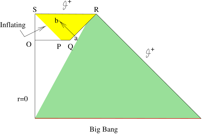
Figure 6.2: A Penrose diagram for local inflation (adapted from [99] ). The arrow (ab) denotes a radially directed null-geodesic going from the normal background space time to the anti-trapped space time inside the patch. Shading represents anti-trapped regions.

Fig. 6.2 shows a Penrose diagram for an embedding that violates the weak energy condition. Here, at the beginning of inflation, $x_{\rm p}^{\rm inf}$ is represented by line OQ and $x_{\rm mas}^{\rm inf}$ is represented by line OP. An inflating patch is pictured to develop within some region inside the background (polygon OQRS in Fig. 6.2). In the inflationary patch, they assume a different Hubble parameter ${\rm H}_{\rm inf}$ and assume the size of this patch must be $\mbox{$x_{\rm p}^{\rm inf}$}>1/\mbox{${\rm H}_{\rm inf}$}$. This assumption can be justified by requiring the patch to be stable against perturbations and will be discussed further in the next section. By Eq. (6.12) it also implies $\mbox{$x_{\rm mas}^{\rm inf}$}=1/\mbox{${\rm H}_{\rm inf}$}$ for $\Omega=1$. If the patch is to be set up by causal processes then we would expect it to be smaller than the background Hubble horizon, $\mbox{$x_{\rm p}^{\rm inf}$}<\mbox{$1/{\rm H}_{\rm bg}$}$. These conditions combined imply $\mbox{$x_{\rm mas}^{\rm bg}$}=\mbox{$1/{\rm H}_{\rm bg}$}>\mbox{$x_{\rm p}^{\rm inf}$}>\mbox{$x_{\rm mas}^{\rm inf}$}$. As such the region between $x_{\rm mas}^{\rm bg}$ and $x_{\rm p}^{\rm inf}$ is normal with respect to the BG-region and the region between $x_{\rm p}^{\rm inf}$ and $x_{\rm mas}^{\rm inf}$ is anti-trapped with respect to the inflating patch. Thus an in-going null ray will go from a negative divergence region to a positive divergence region. Based on Eq. (6.1) this leads to a violation of the weak energy condition. Due to this fact, in [99] they conclude that the only way to avoid this violation is to have $\mbox{$x_{\rm p}^{\rm inf}$}>\mbox{$1/{\rm H}_{\rm bg}$}$ which may be impossible or at least very difficult to come about through causal processes.

Although this analysis assumed a homogeneous background, the general result of [99] was that if the inflationary patch contained a MAS then it must be larger than the background MAS. One of the main aims of this article is to further examine the implications this has for a causal embedding of an inflationary patch.

Our first observation is that there is an embedding consistent with both causality and the weak energy condition, in particular

$$\mbox{$x_{\rm p}^{\rm bg}$},\mbox{$x_{\rm mas}^{\rm inf}$}>\mbox{$x_{\rm p}^{\rm inf}$}\,.$$ (6.13)

Since $x_{\rm p}^{\rm inf}$ in Eq. (6.13) is smaller than $x_{\rm p}^{\rm bg}$, it implies consistency with causality. A region which is smaller than its MAS will have no anti-trapped surfaces. Thus in our proposed embedding Eq. (6.13), the INF-BG boundary is between two normal regions. As such, provided $\mbox{$\theta^{\rm inf}$}]_{\rm boundary}$ is sufficiently smaller than $\mbox{$\theta^{\rm bg}$}]_{\rm boundary}$, the weak energy condition is satisfied. One interesting feature of the embedding Eq. (6.13) is that for $\mbox{$\Omega_{\rm inf}$}<1$ it is acceptable for $\mbox{$x_{\rm p}^{\rm inf}$}>1/{\rm H}_{\rm inf}$.

As inflation proceeds, $\mbox{$\Omega_{\rm inf}$}\rightarrow 1$ and so $\mbox{$x_{\rm mas}^{\rm inf}$}\rightarrow\mbox{$1/{\rm H}_{\rm inf}$}$. One of the main features of inflation is that modes of a matter perturbation become larger than the Hubble radius as the Universe expands. It follows that eventually $\mbox{$x_{\rm p}^{\rm inf}$}>\mbox{$1/{\rm H}_{\rm inf}$},\mbox{$x_{\rm mas}^{\rm inf}$}$ will need to occur. This will not cause violation of the weak energy condition provided that $\mbox{$x_{\rm p}^{\rm inf}$}>\mbox{$x_{\rm mas}^{\rm bg}$}$ at that time.

Fig. 6.3 shows a Penrose diagram of the proposed embedding. At point T in the figure, $\mbox{$x_{\rm p}^{\rm inf}$}=\mbox{$x_{\rm mas}^{\rm bg}$}$ and at point P, $\mbox{$x_{\rm p}^{\rm inf}$}=\mbox{$x_{\rm mas}^{\rm inf}$}$.

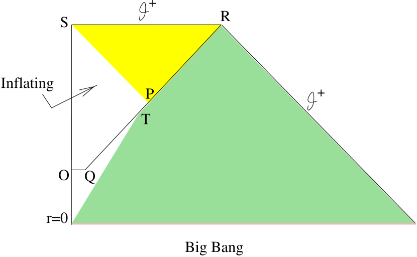
Figure 6.3: A Penrose diagram for local inflation with an embedding that does not violate the weak energy condition and is not acausal.

As can be seen the anti-trapped region develops in the patch only after the patch has become greater than the background MAS.

There is another embedding which does not violate the weak energy condition, in this case for $\mbox{$\Omega_{\rm bg}$}>1$, but it proves not to be as useful,

$$\mbox{$x_{\rm mas}^{\rm inf}$},\mbox{$x_{\rm mas}^{\rm bg}$}<\mbox{$x_{\rm p}^{\rm inf}$}<\mbox{$1/{\rm H}_{\rm bg}$}\,.$$ (6.14)

This solution is restricted by the upper limit on $\Omega_{\rm bg}$ that gives a lower limit (from Eq. 6.12) of $\mbox{$x_{\rm mas}^{\rm bg}$}\approx 0.8/\mbox{${\rm H}_{\rm bg}$}$ for $\Omega=2$. As the causal scale $x_{\rm p}^{\rm bg}$ can be only of the order of $1/{\rm H}_{\rm bg}$, such a large inflationary patch may still be acausal.

Additional information about embedding constraints can be obtained through the Israel junction conditions [110]. In [111, 112] conditions were derived for the embedding of one FRW spacetime within another. The Israel junction conditions require the extrinsic curvature on the background side of the boundary to be smaller than the extrinsic curvature on the patch side of the boundary if the boundary surface energy density is to be positive. It can then be shown [111, 112] that if the energy density of the background $\rho_{\rm bg}$ is greater than that of the patch $\rho_{\rm inf}$, the Israel junction conditions can be satisfied for an inflationary patch of arbitrary size and geometry with any background geometry. They also show for $\mbox{$\rho_{\rm bg}$}<\mbox{$\rho_{\rm inf}$}$, an embedding consistent with the Israel junction conditions and $\mbox{$x_{\rm p}^{\rm inf}$}<\mbox{$1/{\rm H}_{\rm bg}$}$ requires the background geometry to be closed with the geometry of the inflationary patch arbitrary.

6.3 Dynamic Conditions

An immediate concern with the proposed embedding Eq. (6.13) regards the size of the inflationary patch. As far as the embedding conditions are concerned, the patch size simply must lie below the $x_{\rm mas}$ line in Fig. 1. In particular, for $\mbox{$\Omega_{\rm inf}$}>1$ the inflationary patch size must be $<1/\mbox{${\rm H}_{\rm inf}$}$. However, for $\mbox{$\Omega_{\rm inf}$}<1$, the inflationary patch size can be $>1/\mbox{${\rm H}_{\rm inf}$}$. The primary question which remains is what the minimal initial inflation patch size can be in order to be dynamically stable for inflation to commence. For example, if the initial patch is too small, then large fluctuations initially outside the patch could enter inside at a rate sufficiently fast to destroy the inflationary conditions. In this section, the dynamic conditions necessary for inflation will be examined for both the scalar field and a background radiation component.

6.3.1 Scalar field

For scalar field driven inflation, the general dynamical conditions necessary for a finite spatial patch to initiate and sustain inflation have been considered in [101, 102, 103, 104, 105, 106] and a comprehensive review has been given in [107]. Here the requirements addressed in these works, primarily the review [107], will be systematically examined with emphasis on determining their implications for the minimal initial inflationary patch size. Our considerations of scalar field dynamics will generalize those in the above stated works, which focused on supercooled inflationary dynamics [113, 114, 97], in that here warm inflation dynamics [115] also will be treated.

The classical evolution equation for the scalar inflaton field has the general form

$${\ddot{\phi}}({\bf x},t)+[3{\rm H}+\Gamma]{\dot{\phi}}({\bf x},t)$$ (6.15)

$$- a^{-2}\nabla^{2}\phi({\bf x},t)+\frac{\delta V(\phi)}{\delta\phi({\bf x},t)}=0,$$

where $\Gamma$ is a dissipative coefficient, which represents the effective interaction of the inflaton with other fields. Here and below $\phi({\bf x},t)$ is a classical real number which contains the ensemble average of the quantum and/or thermal fluctuations. In supercooled inflation, it is assumed the inflaton is isolated, in which case $\Gamma=0$. Thus no radiation is produced during inflation and the universe inflates in a supercooled state. On the other hand, in warm inflation the inflaton interacts with other fields, and the $\Gamma{\dot{\phi}}$ term is the simplest representation of their effect on the evolution of the inflaton, with generally $\Gamma>{\rm H}$. Due to these interactions, radiation is dissipated from the inflaton system into the universe throughout the inflation period. In general, $\Gamma$ can vary as a function of the inflaton field mode to which it is associated, but here $\Gamma$ is treated as a constant.

There are two types of potential $V(\phi)$ in Eq. (6.15) that typically are treated in inflationary cosmology, a purely concave potential of the generic form $V\sim m^{2}\phi^{2}+\lambda\phi^{4}$ and a double well potential such as $V\sim(\phi^{2}-m^{2})^{2}$. Our discussion to follow will focus of the former type of potential and at the end we will comment on the case of the double well potential. Furthermore, for most of our discussion it will be adequate to consider the simplest case of a quadratic potential, $V=\frac{1}{2}m^{2}\phi^{2}$. In this case, going to Fourier space where we put the universe in a box

$$\phi({\bf x},t)=\sum_{\bf k}\phi_{\bf k}(t)e^{i{\bf k}\cdot{\bf x}},$$ (6.16)

Eq. (6.15) becomes,

$${\ddot{\phi}}_{\bf k}+[3{\rm H}+\Gamma]{\dot{\phi}}_{\bf k}(t)+a^{-2}k^{2}\phi_{\bf k}(t)+m^{2}\phi_{\bf k}(t)=0,$$ (6.17)

where $k^{2}\equiv|{\bf k}|^{2}$ with ${\bf k}$ the comoving wave-vector and ${\bf k}/a(t)$ the corresponding physical wave-vector at time $t$.

A necessary condition for inflation is that the zero mode $\phi_{{\bf k}=0}$, must have a sufficiently large and long-sustained amplitude so that the potential energy $V=\frac{1}{2}m^{2}\phi_{0}^{2}$ dominates the equation of state of the universe, thereby driving inflation. This leads to the familiar slow-roll conditions, which require the curvature of the potential to be sufficiently flat so that Eq. (6.17) for the zero mode becomes first order in time

$${\dot{\phi}}_{0}=-\frac{dV(\phi)/d\phi_{0}}{3{\rm H}+\Gamma}.$$ (6.18)

The dynamic initial condition problem is that the above requirements should not be too special and in particular should not violate causality. The most acute initial condition problem discussed in [107] and related works is that generally the initial inflaton field configuration will be very inhomogeneous, thus considerable contribution of gradient energy ($(\nabla\phi)^{2}$) should be present. In its own right, the gradient term for comoving mode ${\bf k}$ has energy density $\rho_{\nabla}=({\bf k}^{2}/2a^{2})\phi_{\bf k}^{2}$ and equation of state $p_{\nabla}=-\rho_{\nabla}/3$. From the scale factor equation

$$\frac{\ddot{a}}{a}=-\frac{4\pi G}{3}(\rho+3p),$$ (6.19)

the effect of the gradient energy vanishes on the right hand side. As such, any additional contribution from vacuum energy still should drive inflation. However, excited modes with $k/a>3{\rm H}+\Gamma$ not only will possess gradient energy, but based on Eq. (6.17) are under-damped. As such, they also have a kinetic energy contribution $\rho_{\dot{\phi}}\sim{\dot{\phi}}^{2}_{\bf k}$, which has an equation of state $p_{\dot{\phi}}=\rho_{\dot{\phi}}$. If the kinetic energy components of these modes dominates the energy density in the universe, then from Eq. (6.19) inflation will cease to occur.

For the case of supercooled inflation, since $\Gamma=0$, the simplest way to avoid this problem is to require that modes with $k/a\stackrel{{\scriptstyle>}}{{\sim}}{\rm H}$ initially should not be excited. In other words, the inflaton field initially should be smooth up to physical scales larger than $\sim 1/{\rm H}$. However, under general conditions, the causal size of the pre-inflation patch also will be of order the Hubble radius $1/{\rm H}$. As such this homogeneity requirement on the initial inflaton field impinges on being acausal, since this condition essentially requires initially smooth conditions up to the causal scale.

To treat excited modes with $k/a>{\rm H}$ in the supercooled inflation case, the initial condition dynamics are much more complicated. A simple analytical method applied to this situation is the effective density approximation presented in [101, 105] and reviewed in Sec. 7.2 of [107]. In this approach, the inhomogeneities of the inflaton are treated in determining its evolution, but the effect of these inhomogeneities on the metric is only treated in the Friedmann equation through homogeneous terms that represent the effective gradient and kinetic energy densities as

$$\left(\frac{\dot{a}}{a}\right)^{2}\equiv{\rm H}^{2}=\frac{8\pi G}{3}\left[\frac{1}{2}{\dot{\phi}}_{0}^{2}+\frac{1}{2}m^{2}\phi_{0}^{2}\right.+$$

$$\left.\frac{1}{2}\sum_{\bf k}[{\dot{\phi}}_{\bf k}^{2}+(\frac{{\bf k}^{2}}{a^{2}}+m^{2})\phi_{\bf k}^{2}]+\rho_{r}\right]-\frac{K}{a^{2}}.$$ (6.20)

For initial field configurations with sufficiently excited $k/a>{\rm H}$ modes so that their gradient energies dominate the equation of state of the universe, the effective density approximation indicates the Friedmann and inflaton evolution equations are highly coupled. In particular, the Hubble parameter will be dominated by the gradient energy term and this will act back on the inflaton evolution through the $3{\rm H}{\dot{\phi}}$ term. Furthermore, the initially large gradient terms also can in turn induce large kinetic energy in the modes. The outcome found in [101, 105, 107] (see also [103]) for this case is that the universe expansion is non-inflationary. On the other hand, for the excited $k/a>{\rm H}$ modes with smaller amplitudes, their evolution will be oscillatory and once again the universe expansion is non-inflationary. For either of these two possibilities, this approximation method finds that after an initial period of detaining the universe in a non-inflationary regime, the effect of these higher modes becomes negligible. At this point the remaining vacuum energy dominates and eventually inflation proceeds.

Numerical simulations [104, 105] which exactly treat the effects on the metric due to the inhomogeneities in the inflaton field, in fact, do not support this final conclusion of the effective density approximation. Instead, the simulations find that once modes with $k/a>{\rm H}$ are sufficiently excited, inflation generally does not occur or is highly suppressed. Although the final conclusion of the effective density approximation was incorrect, it at least indicated that there is nontrivial interplay between the inflaton and metric evolution equations once significant short distance inhomogeneities are present in the inflaton field.

In contrast to the supercooled case, once $\Gamma>{\rm H}$, the effective density approximation indicates that for modes with $\Gamma>k/a>{\rm H}$, there is almost no feedback between the inflaton and Friedmann equations. The evolution equation for these inflaton modes is

$$\Gamma\dot{\phi}_{\bf k}(t)=\left[\frac{{\bf k}^{2}}{a^{2}}+m^{2}\right]\phi_{\bf k}(t),$$ (6.21)

and in particular is independent of ${\rm H}$. This in turn implies all these modes are over-damped. As such, they only contribute gradient energy to the equation of state of the universe, which alone is ineffective in preventing inflation. Thus up to the predictions of the effective density approximation, in contrast to the supercooled case, in this warm inflation case modes with $k/a<\Gamma$ show little coupling between the inflaton and Friedmann equations. It is evident that dynamics with a $\Gamma{\dot{\phi}}$ damping term should have qualitative differences for the initial condition problem compared to the case with $\Gamma=0$. In particular, modes of physical wavelength smaller that the Hubble radius $1/{\rm H}$ but larger than $1/\Gamma$ could still be substantially excited without destroying entrance into inflation. This implies inflationary patch sizes smaller than the Hubble radius may be dynamically stable in sustaining inflation and based on the results of Sec. 6.2, they also provide consistent spacetime embeddings, especially for $\mbox{$\Omega_{\rm inf}$}<1$. Furthermore, studies of warm inflation [115, 116, 117], including the first principles quantum field theory model [118], generally find that to obtain adequate inflationary e-folds, $N_{e}\stackrel{{\scriptstyle>}}{{\sim}}60$, it requires $\Gamma\approx N_{e}m^{2}/{\rm H}$ with $m\stackrel{{\scriptstyle>}}{{\sim}}{\rm H}$ so that $\Gamma\stackrel{{\scriptstyle>}}{{\sim}}N_{e}{\rm H}$ and thus $1/\Gamma\ll 1/{\rm H}$. As such, for warm inflationary conditions this simple analysis suggests that the smoothness requirement on the initial inflationary patch is at scales much smaller than the Hubble radius $1/{\rm H}$, which therefore imposes no violation of causality.

These considerations can be extended to the more complicated situation where the inflaton evolution equation has nonlinear terms, such as the $\phi^{4}$ interaction term. For supercooled inflation, the effect of such interactions has been considered from the perspective of mode mixing for some special cases in [102, 103] and through computer simulations of scalar fields in one spatial dimension in [104, 105]. Up to the scope of these works, their analysis concludes that nonlinear interactions do not present any additional complications to the initial condition problem. For the warm inflation case, this conclusion can be stated in more general terms. In particular, the dissipative coefficient $\Gamma$ completely damps the evolution, thus suppressing mode mixing, of all modes with $k/a<\Gamma$. As such, initially excited modes with $k/a<\Gamma$ will evolve independently within the time scales relevant to the initial period when inflation begins. The only effect of excited modes with $k/a<\Gamma$ is to contribute gradient energy to the equation of state of the universe, and this alone is ineffective in suppressing inflation. Therefore, provided the inflaton field also initially maintains some vacuum energy, no aspect of the inflaton’s dynamics in the early period acts to circumvent entrance into the inflation phase.

Although the above discussion addressed the main impediment in scalar field dynamics that can prevent inflation, there are a few smaller concerns worth mentioning here. One detail treated in [107] is inflaton initial conditions with large kinetic energy. For $\Gamma=0$, it is shown in [107] that this problem is self-correcting, and so should not pose a major barrier in entering into the inflation phase. For $\Gamma>{\rm H}$, the severity of this problem diminishes further since this damping term is an additional effect that helps suppress the initial kinetic energy. Another secondary detail is that above we only treated concave potentials. For double well potentials, $V\sim(\phi^{2}-m^{2})^{2}$, as in the case of new inflation [114], inflation requires the field to be well localized at the top of the potential hill $\phi=0$ and almost at rest. These requirements are necessary, otherwise as found in various studies [119], the field can easily break up into several small domains with randomly varying signs of the amplitude. For the supercooled case, new inflation, the basic conclusion about the initial conditions required for inflation has been that they are not very robust [119, 120, 107]. The inclusion of a dissipative term $\Gamma>{\rm H}$ will not necessarily improve this situation. On the one hand, such a term helps considerably to damp kinetic energy, thus allowing the inflaton to remain at the top of the hill longer and drive inflation. On the other hand, if such a damping term arises too early before inflation is to begin, since it freezes the evolution of excited inflaton modes, it could prevent the initial inflaton field configuration from equilibriating to $\phi=0$.

Finally in the above discussion $\Gamma\neq 0$ generally represented warm inflation dynamics, although even for supercooled inflation, if radiation is present at the onset of inflation, such as in the new [114] and thermal [121] inflation pictures, the effective evolution of the inflaton could have a damping term of the form $\Gamma{\dot{\phi}}$. Since our focus is on the initial phase at the onset of inflation, it is possible the effect of such damping terms also may be applicable to the initial condition problem in some supercooled inflation models.

6.3.2 Radiation component

So far we only considered the inflaton field system, but in addition the universe could possess some background component of radiation energy density, $\rho^{\rm bg}_{\rm r}$. To realize inflation, minimally it requires the vacuum energy density $\rho_{\rm v}$ to dominate in the patch, $\mbox{$\rho^{\rm bg}_{\rm r}$}<\rho_{\rm v}$. If initially $\rho^{\rm bg}_{\rm r}$ is larger than $\rho_{\rm v}$, expansion of the universe will red-shift the radiation. Thus provided the vacuum energy sustains itself during this early period, inflation eventually will start. This is the standard new and warm inflation pictures.

One could imagine that in some small patch inside a larger causally created spatial region, the inflaton field configuration is reasonably smooth and is sustaining a sizable vacuum energy of magnitude

$$\rho_{\rm v}\approx\mbox{$\rho^{\rm bg}_{\rm r}$}.$$ (6.22)

As the universe expands $\rho^{\rm bg}_{\rm r}$ decreases and provided $\rho_{\rm v}$ sustains itself, inflation will begin in the patch. However at this moment, there could be large energy fluctuations in the radiation bath or other fields that are just outside the putative inflationary patch. One would like to understand how probable it is for such a situation to curtail the inflation that had started in the patch.

To answer this question based solely on causality considerations, one should consider the case of a perturbation starting on the patch boundary and moving across the patch at the speed of light, and make the extreme assumption that as the perturbation overruns regions of the inflation patch, those regions convert back to being non-inflating. The question is what minimal initial inflationary patch size is needed so that its expansion under inflation is faster than its contraction due to the impinging perturbations. For the case of flat geometry $\Omega=1$, this question was addressed in [107] and they concluded that the patch size should be at least 3 times the Hubble radius in order for inflation to succeed in enlarging the patch. For a general $\Omega$, we can address this question by evaluating the maximum distance a perturbation can travel in the patch between the initial $t_{i}$ and final $t_{f}$ time of inflation

$$x_{\rm pert}=a(t)\int_{t_{i}}^{t_{f}}a^{-1}\,dt.$$ (6.23)

Note that since $a$ is growing rapidly, there is negligible error in taking $t_{f}\rightarrow\infty$ which implies $x_{\rm pert}$ essentially is the event horizon. We have examined Eq. (6.23) for a variety of supercooled and warm inflation models and generally find $x_{\rm pert}\approx\mbox{$x_{\rm mas}$}$.

Thus in the most ideal case, an inflationary patch smaller than the event horizon can not be stable. Here an important point of syntax should be noted, that the generic size here is the event horizon and not the Hubble radius, although for the flat case, $\Omega=1$, both are of the same order. The above is the ideal bound based on causality. However, realistic dynamics also must be considered.

One case which corresponds to external perturbations entering into an initially inflating patch is the case treated in Subsect. IIIA of the mixing of high wavenumber modes. For the inflaton field interacting with itself or with other fields, we argued above that if a dissipative term of the form $\Gamma{\dot{\phi}}$ is present in the inflaton effective evolution equation, then mode mixing up to wave-numbers $k/a<\Gamma$ will not occur within the time scale relevant to the initial condition problem.

In terms of the radiation bath, suppose a small vacuum dominated inflationary regime emerges, which is immersed inside a larger region containing radiation and gradient energy density. Since the inflationary patch has negative pressure, the surrounding radiation will flow into it. The degree to which the pressure differences are significant to this process depends on the magnitudes of the radiation, gradient and vacuum energies in both regions as well as detailed dynamical considerations[111, 122]. Nevertheless, suppose the radiation tries to become uniform over the entire region, including the patch. Since the patch started to inflate, it meant that initially $\rho_{\rm v}\stackrel{{\scriptstyle>}}{{\sim}}\mbox{$\rho^{\rm bg}_{\rm r}$}$. As time commences, provided $\rho_{\rm v}$ remains constant, since expansion of the background will decrease $\rho^{\rm bg}_{\rm r}$, it means the amount of radiation that flows into the inflationary patch will be less than $\rho_{\rm v}$. Thus irrespective of whether the inflaton dynamics is supercooled or warm, the patch should sustain a type of warm inflation due to this influx of radiation from the regions that surround it.

A thorough understanding of the initial condition dynamics in presence of a background radiation component is complicated. To our knowledge, no quantitative analysis has been done along these lines. The review [107] only illustrated the problem with the example quoted above Eq. (6.23) based on causality considerations but offered no dynamical examples with respect to a background radiation component. Here we have offered one scenario where the background radiation component should not prevent inflation from occurring. In particular, this example demonstrates that causality bounds on the rate at which radiation or other energy fluctuations enter the patch are not the only aspect of this problem. In addition, the magnitude of the entering radiation must be adequately large to overwhelm the vacuum energy. We have offered arguments above that indicate this latter requirement is not generic.

6.4 Dynamical effects on embedding

As discussed in Sec. 6.2, a causally favourable embedding requires the inflationary patch to start smaller than the background MAS and then grow larger than it. A minimum condition for this to happen is that the particle horizon of the background eventually becomes greater than the background MAS.

For $p=\omega\rho$, the particle horizon is given by [7]

$$d(t)=\frac{1}{H}\int_{0}^{1}\frac{dx}{\left[x^{2}(1-\Omega(t))+\Omega(t)x^{1-3w}\right]^{1/2}}.$$ (6.24)

Comparing this equation with Eq. (6.12) it can be seen that the particle horizon will only become greater than the MAS if $\omega<1/3$. This condition was also noted in [123] from a slightly different perspective. There the patch was taken to start larger than the background MAS.

It follows that our proposed embedding will not work for a pure radiation background which has $\omega=1/3$. However, in general the background will consist of radiation and an inhomogeneous scalar field. As discussed in Sec. 6.3, the gradient energy of the scalar field has $\omega=-1/3$ and the potential energy has $\omega=-1$ while the kinetic energy has $\omega=1$. It follows that if the background is gradient dominated our causal embedding scheme will be viable, whereas our scheme fails if the kinetic term dominates. However, the kinetic energy of the scalar field will be suppressed if the dissipative coefficient $\Gamma$ of Sec. 6.3 is sufficiently large. This is already required inside the putative inflation patch in order to realize inflation. Thus, it is not unreasonable to expect $\Gamma$ in the background region to be of the same magnitude.

6.5 Conclusion

This Chapter has investigated the initial condition problem of inflation from the perspective both of spacetime embedding and inflaton dynamics. Our study has highlighted two attributes of this problem which have not been addressed in other works. First, from the perspective of spacetime embedding, we have observed that the global geometry can play an important role in determining the size of the initial inflationary patch that is consistent with the weak energy condition. Second, from the perspective of inflaton dynamics, we have noted that a $\Gamma{\dot{\phi}}$ damping term could alleviate several problems which traditionally have led to large scale homogeneity requirements before inflation.

The purpose of this Chapter was to note for both these attributes, their salient features with respect to the initial condition problem. In the wake of this, several details emerge that must be understood. Below, we will review the main result we found for both attributes and then discuss the questions that must be addressed in future work.

For a causally generated patch a successful embedding can be achieved if the patch does not contain an anti-trapped region. We have shown that the MAS size can be arbitrarily larger than the Hubble scale provided $\Omega$ is made small enough. So if the patch Hubble horizon is taken as the minimum stable patch size, then the patch does not have to contain an anti-trapped region if $\mbox{$\Omega_{\rm inf}$}<1$. This generalizes the analysis of [99] which was only for $\Omega=1$. However, without the effects of damping, it appears that the event horizon, not the Hubble horizon, is the minimum stable patch size. For the de Sitter case one can see analytically that the event horizon is equal to the MAS size regardless of $\Omega$ and numerical calculations suggest the same is true for power law inflation. However, radiation damping of perturbations could stabilize a patch smaller than the event horizon. In this case an open geometry for the patch would allow the patch not to contain an anti-trapped region and thus allow a causal embedding in an expanding background which does not violate the weak energy condition. Eventually the patch should develop a MAS within it, but by then it could have expanded to be larger than the background MAS.

For the dynamics problem, with respect to the scalar field the new consideration was the effect of a $\Gamma{\dot{\phi}}$ damping term. We found that such a term could suppress many of the effects from initial inhomogeneities of the inflaton, which in studies traditionally done without this term lead to important impediments to entering the inflation regime. It appears evident that inclusion of such a damping term will lead to qualitative differences in the initial condition problem. The most interesting outcome is initial inflationary patches smaller than the Hubble radius $1/{\rm H}$ may be able to inflate.

This Chapter examined the consequences of damping terms but did not delve into their fundamental origin. For the cosmological setting, such damping terms are typically associated with systems involving a scalar field interacting with fields of a radiation bath. In this case, such damping terms have been found in first principles calculations for certain warm inflation models [118], although more work is needed along these lines. It is worth noting here that in the early stages of certain supercooled inflaton scenarios where radiation is present, in particular new [114] and thermal [121] inflation, a careful examination of the dynamics may reveal damping terms similar to this. Since the initial stages are the crucial period for the initial condition problem, if further study supports the importance of such damping terms, it may be useful to better understand damping effects also in such scenarios.

Since the most suggestive situation for the damping terms is where in addition a radiation component is present in the universe, in Subsect. IIIB we also studied the effects of this component on the initial condition problem. Specifically we studied the case most suggestive for the initial stages of new and warm inflation, where a small inflation patch is submerged inside a larger radiation dominated spatial region. Our main observation has been that the minimal condition for the patch to inflate is that its vacuum energy density must be larger than the background radiation energy density. Provided the vacuum energy sustains itself, since expansion of the universe will dilute the radiation energy density, it is not clear-cut that the external radiation energy can act with sufficient magnitude to impede inflation inside the patch.

We have shown that the gradient terms, due to the inhomogeneous scalar field in the background space time, make it possible for the patch boundary to overtake the background MAS. However the kinetic energy of the scalar field must not be dominant for this to happen. This can be ensured by including a damping term in the scalar field equation.

Chapter 7 Conclusions

In this Chapter the results of the thesis are summarised and current and possible extensions of the work are discussed.

In Chapter 2 adiabatic and entropy perturbations from multi-field models were studied [1]. A general perturbation was decomposed into components parallel (adiabatic) and perpendicular (entropy) to the background trajectory. We derived the evolution equations for the entropy and adiabatic perturbations. From these equations it was evident that on large scales the evolution of the adiabatic perturbation is driven by the entropy perturbation, whereas the entropy is not driven by the adiabatic perturbation. We found that inflationary potentials that have a small effective entropy mass can generate non-negligible entropy perturbations. Also, it was shown that it is only for a non-straight background trajectory that the entropy will source the adiabatic component on large scales.

We also analysed how correlations in the adiabatic and entropy components can arise in multi-field models. We found that when the adiabatic component is driven by the entropy component, it becomes correlated with it. The magnitude of this correlation depends on the relative magnitude of the homogeneous and inhomogeneous solutions of the adiabatic evolution equation. The magnitude of the isocurvature perturbation, in the radiation era, depends on the magnitude of the entropy perturbation at the end of inflation and the details of how the transition from the inflation to radiation era takes place. But, on large scales, it is independent of the adiabatic perturbation.

We analysed the non-interacting double inflation model using our decomposition. Our approach was useful in identifying the reason for the features of the resulting power spectra during the radiation era.

The question of whether preheating could affect the spectrum of perturbations on scales relevant to structure formation was addressed in Chapter 3 [1, 2]. A range of models that might have this property were examined. A potential which has efficient preheating and does not suppress the entropy perturbation during inflation was shown to be necessary for preheating to affect large scale structure.

We found that when the mass of the entropy field is larger than the Hubble parameter during inflation, the entropy perturbation will be exponentially suppressed and so preheating will not be able to effect large scale structure. We also found that our new entropy evolution equation was much more numerically robust, in tracking this suppression, when compared to using the usual field perturbation equations and constructing the entropy perturbation algebraically.

The formalism discussed in Chapter 2 (which originally appeared in [1]) has subsequently been extended by Bartolo et al. [78]. They derived generic slow roll expressions for the adiabatic and entropy perturbation. One question that we believe still needs to be resolved is how the entropy perturbation is transferred from the inflation to the radiation era. When there are couplings between the scalar fields, how these couplings influence the transfer is still not properly understood.

In Chapter 4 we studied the effect of including correlated adiabatic and entropy perturbations on parameter estimation using the CMB [3]. We proposed a generic form for the initial power spectra which should encompass a broad range of two-field inflation models. We then modified the program CMBFAST and showed how considerable savings in computation can be achieved by using library spectra.

We found that the current CMB data was consistent with a correlated CDM entropy perturbation of as high as twice the magnitude of the adiabatic perturbation. We also found a degeneracy between the primordial slope and the amount of correlated CDM entropy perturbation.

Subsequently Bartolo, et al. [124] have used the formalism we developed in [1] to derive consistency relations between the scalar and tensor slopes for two field models. These consistency relations could provide a detectable signature for two-field inflation models in the CMB.

In Chapter 5 we studied the the effect of having an extra spatial dimension on density perturbations in the brane world scenario [4]. We analysed super-Hubble scalar perturbations using a covariant approach, and found that they evolve differently from general relativity due to bulk effects. The metric perturbation is no longer constant on super-Hubble scales during inflation and high energy radiation.

We examined how the bulk Weyl curvature can be treated as an additional fluid on the brane with possibly non-adiabatic perturbations. We showed that on large scales the density perturbations on the brane are described by a closed system of equations, while on small scales there is no equation describing the evolution of the anisotropic pressure of the projected Weyl curvature on the brane and so the full five dimensional problem has to be studied. Subsequently Langlois et al. [85] have shown how even the SW effect cannot be computed on the brane without solving the 5D equations.

In Chapter 6 we examined how non-linear inhomogeneities effected the start of inflation [5]. We extended previous work to show that even for a non-flat geometry it was not possible to initiate inflation if there were perturbations on a scale smaller than the Hubble horizon.

We then examined the effect of including a damping term due to decay of the inflaton into radiation during inflation as in the ‘warm inflation’ model. We found this damping term set a new minimum wave length for the non-linear perturbations that could be smoothed by inflation. This minimum wave-length could be smaller than the Hubble distance and so this allows a causal mechanism to be responsible for the initial configuration of the inflationary patch.

Bibliography

- [1] C. Gordon, D. Wands, B. A. Bassett and R. Maartens, Phys. Rev. D 63 023506 (2001).
- [2] B. A. Bassett, C. Gordon, R. Maartens and D. I. Kaiser, Phys. Rev. D 61 061302 (2000).
- [3] L. Amendola, C. Gordon, D. Wands and M. Sasaki, astro-ph/0107089.
- [4] C. Gordon and R. Maartens, Phys. Rev. D 63 044022 (2001).
- [5] A. Berera and C. Gordon, Phys. Rev. D 63 063505 (2001).
- [6] C. Gordon, IEEE Transactions on Geoscience and Remote Sensing 38 608 (2000).
- [7] E. W. Kolb and M. S. Turner, The Early Universe, Addison-Wesley (1990); M. S. Longair, Galaxy Formation, Springer (1998).
- [8] A. R. Liddle and D. H. Lyth, Cosmological inflation and large-scale structure, Cambridge University Press (2000).
- [9] C. L. Bennett et al., Astrophys. J. 464 L1 (1996).
- [10] W. Stoeger et al., Astrophys. J. 443 L1 (1995).
- [11] V. F. Mukhanov, H. A. Feldman and R. H. Brandenberger, Phys. Rept. 215 203 (1992).
- [12] C. B. Netterfield et al., astro-ph/0104460.
- [13] N. W. Halverson et al., astro-ph/0104489.
- [14] A. T. Lee et al., astro-ph/0104459.
- [15] A. D. Linde, Particle Physics And Inflationary Cosmology, Harwood (1990).
- [16] N. W. Mac Lachlan, Theory and applications of the Mathieu functions, Dover (1961).
- [17] L. Kofman, A. D. Linde and A. A. Starobinsky, Phys. Rev. Lett. 73 3195 (1994).
- [18] L. Kofman, A. D. Linde and A. A. Starobinsky, Phys. Rev. D 56 3258 (1997).
- [19] N. Arkani-Hamed, S. Dimopoulos and G. R. Dvali, Phys. Lett. B 429 263 (1998).
- [20] L. Randall and R. Sundrum, Phys. Rev. Lett. 83 4690 (1999).
- [21] L. J. Randall and R. Sundrum, Nucl. Phys. B 557 79 (1999).
- [22] R. Maartens, gr-qc/0101059.
- [23] J. García-Bellido and D. Wands, Phys. Rev. D 52 6739 (1995); J. García-Bellido and D. Wands, Phys. Rev. D 53 5437 (1996).
- [24] S. Tsujikawa and H. Yajima, hep-ph/0007351.
- [25] H. Kodama and T. Hamazaki, Prog. Theor. Phys. 96 949 (1996); T. Hamazaki and H. Kodama, Prog. Theor. Phys. 96 1123 (1996).
- [26] W. Hu, Phys. Rev. D 59 021301 (1999).
- [27] D. Wands, K. A. Malik, D. H. Lyth and A. R. Liddle, Phys. Rev. D 62 043527 (2000).
- [28] B. A. Bassett, F. Tamburini, D. I. Kaiser, and R. Maartens, Nucl. Phys. B 561 188 (1999).
- [29] B. Bassett, D. Kaiser, and R. Maartens, Phys. Lett. B 455 84 (1999.
- [30] F. Finelli and R. Brandenberger, Phys. Rev. Lett. 82 1362 (1999).
- [31] M. Sasaki and E. D. Stewart, Prog. Theor. Phys. 95 71 (1996).
- [32] A. A. Starobinsky, Pis’ma Zh.Éksp. Teor. Fiz. 42 45 (1985) [JETP Lett. 42 51 (1985)].
- [33] D. S. Salopek, Phys. Rev. D 52 5563 (1995); T. T. Nakamura and E. D. Stewart, Phys. Lett. B 381 413 (1996).
- [34] M. Sasaki and T. Tanaka, Prog. Theor. Phys. 99 763 (1998).
- [35] D. H. Lyth and A. Riotto, Phys. Rep. 314 1 (1999).
- [36] D. Polarski and A. A. Starobinsky, Nucl. Phys. B 385 623 (1992).
- [37] D. Polarski and A. A. Starobinsky, Phys. Rev. D 50 6123 (1994).
- [38] A. A. Starobinsky and J. Yokoyama, gr-qc/9502002.
- [39] V. F. Mukhanov and P. J. Steinhardt, Phys. Lett. B 422 52 (1998).
- [40] J. Lesgourgues, Nucl. Phys. B 582 593 (2000). [
- [41] A. D. Linde, Phys. Lett. B 158 375 (1985); D. Seckel and M. S. Turner, Phys. Rev. D 32 3178 (1985); L. A. Kofman, Phys. Lett. B 173 400 (1986); A. D. Linde and L. A. Kofman, Nucl. Phys. B 282 555 (1987); D. S. Salopek, Phys. Rev. D 45 1139 (1992); A. D. Linde and V. F. Mukhanov, Phys. Rev. D 56 535 (1997). M. Bucher and Y. Zhu, Phys. Rev. D 55 7415 (1997); P. J. E. Peebles, Astrophys. J. 510 523 and 531 (1999); A. R. Liddle and A. Mazumdar, Phys. Rev. D 61 123507 (2000).
- [42] H. Kodama and M. Sasaki, Int. J. Mod. Phys. A 1 265 (1986); P. J. E. Peebles, Astrophys. J. 315 L73 (1987); T. Chiba, N. Sugiyama, and Y. Suto, Astrophys. J. 429 427 (1994).
- [43] H. Kodama and M. Sasaki, Int. J. Mod. Phys. A2 491 (1987); J. R. Bond and G. Efstathiou, Mon. Not. R. Astron. Soc. 218 103 (1986).
- [44] M. Bucher, K. Moodley and N. Turok, Phys. Rev. D 62 083508 (2000).
- [45] D. Langlois, Phys. Rev. D 59 123512 (1999).
- [46] M. A. Bucher, K. Moodley, and N. G. Turok, astro-ph/0007360.
- [47] D. Langlois and A. Riazuelo, Phys. Rev. D 62 043504 (2000).
- [48] J. R. Bond and G. Efstathiou, Mon. Not. R. Astron. Soc. 222 33 (1987); W. Hu, E. Bunn, and N. Sugiyama, Astrophys. J. 447 L59 (1995); R. Stompor, A. J. Banday, and K. M. Gorski, Astrophys. J. 463 8 (1996); T. Kanazawa, M. Kawasaki, N. Sugiyama, and T. Yanagida, Prog. Theor. Phys. 102 71 (1999); K. Enqvist and H. Kurki-Suonio, Phys. Rev. D 61 043002 (2000); E. Pierpaoli, J. Garcia-Bellido, and S. Borgani, JHEP 10 015 (1999); K. Enqvist, H. Kurki-Suonio, and J. Valiviita, Phys. Rev. D 62 (2000) 103003.
- [49] K. Enqvist, H. Kurki-Suonio and J. Valiviita, Phys. Rev. D 62 103003 (2000).
- [50] K. A. Malik and D. Wands, Phys. Rev. D 59 123501 (1999).
- [51] J. M. Bardeen, Phys. Rev. D 22 1882 (1980).
- [52] J. Hwang, Astrophys. J. 427 542 (1994).
- [53] M. Bruni, G. F. R. Ellis and P. K. S. Dunsby, Class. Quantum Grav. 9 921 (1992).
- [54] R. Durrer, Fundamentals of Cosmic Physics 15 209 (1994).
- [55] H. Kodama and M. Sasaki, Prog. Theor. Phys. Suppl. 78 1 (1984).
- [56] M. Sasaki, Prog. Theor. Phys. 76 1036 (1986); V. F. Mukhanov, Zh.Éksp. Teor. Fiz. 94 1 (1988) [Sov. Phys. JETP 68 1297 (1988)].
- [57] A. Taruya and Y. Nambu, Phys. Lett. B 428 37 (1998).
- [58] V. Lukash, Zh. Eksp. Teor. Fiz. 79 1601 (1980) [Sov. Phys. JETP 52 807 (1980)].
- [59] D. H. Lyth, Phys. Rev. D 31 1792 (1985).
- [60] J. M. Bardeen, P. J. Steinhardt and M. S. Turner, Phys. Rev. D 28 679 (1983).
- [61] J. Martin and D. J. Schwarz, Phys. Rev. D 57 3302 (1998).
- [62] A. R. Liddle and D. H. Lyth, Phys. Rep. 231 1 (1993).
- [63] F. Finelli and R. H. Brandenberger, Phys. Rev. D 62 (2000) 083502.
- [64] J. M. Stewart and M. Walker, Proc. R. Soc. Lond. A 341 49 (1974).
- [65] A. Mazumdar and L. E. Mendes, Phys. Rev. D 60 103513 (1999).
- [66] B. A. Bassett and F. Viniegra, Phys. Rev. D 62 043507 (2000).
- [67] K. Jedamzik and G. Sigl, Phys. Rev. D 61 023519 (2000); P. Ivanov, Phys. Rev. D 61 023505 (2000)/
- [68] A. R. Liddle, D. H. Lyth, K. A. Malik and D. Wands, Phys. Rev. D 61 103509 (2000).
- [69] N. D. Birrell and P. C. W. Davies, Quantum fields in curved space Cambridge University Press (1982).
- [70] J. P. Zibin, R. H. Brandenberger and D. Scott, Phys. Rev. D 63 043511 (2001).
- [71] S. Tsujikawa, B. A. Bassett, and F. Viniegra, JHEP 08 019 (2000).
- [72] H. Müller and C. Schmid, gr-qc/9412022.
- [73] B. A. Bassett, G. Pollifrone, S. Tsujikawa and F. Viniegra, Phys. Rev. D 63 103515 (2001).
- [74] M. S. Turner and L. W. Widrow, Phys. Rev. D 37 2743 (1988).
- [75] M. Tegmark, M. Zaldarriaga and A. J. Hamilton, Phys. Rev. D 63 (2001) 043007.
- [76] P. de Bernardis et al., astro-ph/0105296; R. Stompor et al., astro-ph/0105062; C. Pryke et al., astro-ph/0104490; X. Wang et al., astro-ph/0105091.
- [77] J. Hwang and H. Noh, Phys. Lett. B 495 277 (2000).
- [78] N. Bartolo, S. Matarrese and A. Riotto, astro-ph/0106022.
- [79] R. Trotta, A. Riazuelo and R. Durrer, astro-ph/0104017.
- [80] J. R. Bond, A. H. Jaffe and L. Knox, Ap. J. 533 (2000).
- [81] U. Seljak and M. Zaldarriaga, Ap. J. 469 (1996).
- [82] R. Maartens, D. Wands, B. A. Bassett, and I. P. C. Heard, Phys. Rev. D 62 041301R (2000).
- [83] E. J. Copeland, A. R. Liddle and J. E. Lidsey, Phys. Rev. D 64 023509 (2001).
- [84] R. Maartens, Phys. Rev. D 62 084023 (2000).
- [85] D. Langlois, R. Maartens, M. Sasaki and D. Wands, Phys. Rev. D 63 084009 (2001).
- [86] H. Kodama, A. Ishibashi, and O. Seto, Phys. Rev. D 62 064022 (2000); D. Langlois, Phys. Rev. D 62 126012 (2000); D. Langlois, Phys. Rev. Lett. 86 2212 (2001); K. Koyama and J. Soda, hep-th/0108003; S. Mukohyama, Class. Quant. Grav. 17 4777 (2000).
- [87] C. van de Bruck, M. Dorca, R. H. Brandenberger and A. Lukas, Phys. Rev. D 62 123515 (2000); C. van de Bruck, M. Dorca, C. J. Martins and M. Parry, Phys. Lett. B 495 183 (2000).
- [88] D. Langlois, R. Maartens, and D. Wands, Phys. Lett. B 489 259 (2000).
- [89] J. D. Barrow and R. Maartens, gr-qc/0108073.
- [90] K. Maeda and D. Wands, Phys. Rev. D 62 124009 (2000); A. Mennim and R. A. Battye, Class. Quant. Grav. 18 2171 (2001).
- [91] S. Mukohyama, T. Shiromizu, and K. Maeda, Phys. Rev. D 61 024028 (2000).
- [92] P. Binetruy, C. Deffayet, U. Ellwanger, and D. Langlois, Phys. Lett. B 477 285 (2000).
- [93] T. Shiromizu, K. Maeda, and M. Sasaki, Phys. Rev. D 62 024012 (2000).
- [94] J. Cline, C. Grojean, and G. Servant, Phys. Rev. Lett. 83 4245 (1999); L. E. Mendes and A. R. Liddle, Phys. Rev. D 62 103511 (2000); A. Mazumdar, Phys. Rev. D 64 (2001) 027304; A. Mazumdar, Nucl. Phys. B 597 (2001) 561.
- [95] G. F. R. Ellis, J. Hwang and M. Bruni, Phys. Rev. D 40 1819 (1989).
- [96] J. Garriga and M. Sasaki, Phys. Rev. D62 043523 (2000); A. Chamblin, A. Karch and A. Nayeri, Phys. Lett. B 509 163 (2001).
- [97] A. Linde, Phys. Lett. 129B 177 (1983).
- [98] K. Sato, H. Kodama, M. Sasaki, and K. Maeda, Phys. Lett B 108 103 (1982); E. Fahri and A. Guth, Phys. Lett. B 183 149 (1987); S. Blau, E. Guendelman and A. Guth, Phys. Rev. D 35 1747 (1987); E. Fahri, A. Guth, and J. Guven, Nucl. Phys. B 339 417 (1990).
- [99] T. Vachaspati and M. Trodden, Phys. Rev. D 61 023502 (2000).
- [100] M. Trodden and T. Vachaspati, Mod. Phys. Lett. A14 1661 (1999).
- [101] T. Piran, Phys. Lett. B 181 238 (1986).
- [102] J. H. Kung and R. Brandenberger, Phys. Rev. D 40 2532 (1989).
- [103] J. H. Kung and R. Brandenberger, Phys. Rev. D 42 1008 (1990).
- [104] D. S. Goldwirth and T. Piran, Phys. Rev. Lett. 64 2852 (1990).
- [105] D. S. Goldwirth, Phys. Rev. D 43 3204 (1991).
- [106] H. Kurki-Suonio, P. Laguna, and R. A. Matzner, Phys. Rev. D 48 3611 (1993); E. Calzetta and M. Sakellariadou, Phys. Rev. D 45 2802 (1992); T. Chiba, K. Nakao, and T. Nakamura, Phys. Rev. D 49 3886 (1994); O. Iguchi and H. Ishihra, Phys. Rev. D 56 3216 (1997).
- [107] D. S. Goldwirth and T. Piran, Phys. Rept. 214 223 (1992).
- [108] A. K. Raychaudhuri, Phys. Rev. 98 1123 (1955).
- [109] R. M. Wald, General Relativity, University of Chicago Press (1984).
- [110] W. Israel, Nuovo Cim. B 44 1 (1966).
- [111] V. A. Berezin, V. A. Kuzmin and I. I. Tkachev, Phys. Rev. D 36 2919 (1987).
- [112] N. Sakai and K. Maeda, Phys. Rev. D 50 5425 (1994).
- [113] A. H. Guth, Phys. Rev D 23 347 (1981); E. Gliner and I. G. Dymnikova, Sov. Astron. Lett. 1 93 (1975); R. Brout, F. Englert and E. Gunzig, Ann. Phys. 115 78 (1978); R. Brout, F. Englert and P. Spindel, Phys. Rev. Lett. 43 417 (1979); A. A. Starobinsky, Phys. Lett. B 91 154 (1980); L. Z. Fang, Phys. Lett. B 95 154 (1980); E. Kolb and S. Wolfram, Astrophys. J. 239 428 (1980); K. Sato, Phys. Lett. B 99 66 (1981); ibid Mon. Not. R. Astron. Soc. 195 467 (1981); D. Kazanas, Astrophys. J. 241 L59 (1980).
- [114] A. Albrecht and P. J. Steinhardt, Phys. Rev. Lett. 48 1220 (1982); A. Linde, Phys. Lett. 108B 389 (1982).
- [115] A. Berera, Phys. Rev. Lett. 75 3218 (1995); A. Berera, Phys. Rev. D 54 2519 (1996).
- [116] A. Berera, Phys. Rev. D 55 3346 (1997).
- [117] A. N. Taylor and A. Berera, Phys. Rev. D 62 083517 (2000).
- [118] A. Berera, M. Gleiser and R. O. Ramos, Phys. Rev. Lett. 83 (1999) 264; A. Berera, Nucl. Phys. B 585 666 (2000).
- [119] A. D. Linde, Phys. Lett. B 132 317 (1983); A. D. Linde, Phys. Lett. B 162 281 (1985); G. F. Mazenko, W. G. Unruh, and R. M. Wald, Phys. Rev. D 31 273 (1985).
- [120] D. S. Goldwirth, Phys. Lett. B 243 41 (1990).
- [121] D. H. Lyth and E. D. Stewart, Phys. Rev. Lett. 75 201 (1995).
- [122] P. J. Steinhardt, Phys. Rev. D 25 2074 (1982).
- [123] D. H. Coule, Phys. Rev. D 62 124010 (2000).
- [124] N. Bartolo, S. Matarrese and A. Riotto, astro-ph/0107502.